1. INTRODUCTION
Receiver Autonomous Integrity Monitoring (RAIM) (Lee, Reference Lee1986; Parkinson and Axelrad, Reference Parkinson and Axelrad1988) is implemented in Global Navigation Satellite Systems (GNSS) to protect users against potential integrity threats caused, for example, by satellite failures. RAIM not only aims at detecting faults but also at evaluating the integrity risk, which is the probability of undetected faults causing unacceptably large errors in the estimated position (RTCA Special Committee 159, 2004). Hence, both the detector and the estimator influence RAIM performance. This two-part research work describes the design, analysis and evaluation of new methods to determine the optimal detector and estimator, which minimise the integrity risk in RAIM. This paper constitutes Part 1, which focuses on optimal detection methods. Part 2 (Joerger et al., Reference Joerger, Langel and Pervan2015) will address estimator design for integrity risk minimisation.
The core principle of RAIM is to exploit redundant measurements to achieve self-contained fault detection at the user receiver. With the modernisation of the Global Positioning System (GPS), the full deployment of GLONASS, and the emergence of Galileo and BeiDou, an increased number of redundant ranging signals becomes available, which has recently drawn a renewed interest in RAIM. In particular, RAIM can help alleviate requirements on ground monitors. For example, researchers in the European Union and in the United States are investigating Advanced RAIM (ARAIM) for worldwide vertical guidance of aircraft (EU-US Cooperation on Satellite Navigation, 2012).
One of the primary tasks in RAIM is to evaluate the integrity risk, or alternatively, a protection level, which is an integrity bound on the positioning error. Integrity risk evaluation is needed when designing a navigation system to meet predefined integrity requirements, and it is needed operationally to inform the user whether to abort or to pursue a mission. Integrity risk evaluation involves both assessing the fault detection capability and quantifying the impact of undetected faults on position estimation errors.
Both the RAIM detector and the estimator have been investigated in the literature. With regard to fault detection, two RAIM algorithms have been widely implemented over the past 25 years: chi-squared (χ 2) RAIM (also called parity-based or residual-based RAIM (Sturza, Reference Sturza1988; Brown, Reference Brown1992)) and Solution Separation (SS) RAIM (Brenner, Reference Brenner1996; Blanch et al., Reference Blanch, Ene, Walter and Enge2007). Fundamental differences between the two algorithms have been pointed out in Joerger et al. (Reference Joerger, Chan and Pervan2014), but it remains unclear whether SS or χ 2 RAIM provides the lowest integrity risk. In parallel, with regard to estimation, researchers have explored the potential of replacing the conventional Least-Squares (LS) process with a Non-Least-Squares (NLS) estimator to lower the integrity risk in exchange for a slight increase in nominal positioning error (Hwang and Brown, Reference Hwang and Brown2006; Lee, Reference Lee2008; Blanch et al., Reference Blanch, Walter and Enge2012). The resulting methods show promising reductions in integrity risk, but are computationally expensive for real-time implementations.
In response, this two-part research effort provides new methods to determine the optimal detector and estimator in RAIM, which minimise the integrity risk. Optimal design of the detector and of the estimator is respectively tackled in Part 1 (i.e., in this paper) and in Part 2 (i.e., in Joerger et al. (Reference Joerger, Langel and Pervan2015)).
In Section 2 of this paper, the SS and χ 2 RAIM detectors are described using parity space representations, which are essential because the parity vector is the simplest, most fundamental expression of the detection capability. Joerger et al. (Reference Joerger, Chan and Pervan2014) shows that the detection boundaries of SS and χ 2 RAIM respectively describe a polytope and a hyper-sphere in parity space. In addition, these two methods are computationally efficient, which makes them good candidates for real-time navigation applications. However, the circumstances under which SS provides a lower integrity risk than χ 2 RAIM, or vice versa, have yet to be defined.
Multiple implementations of SS and χ 2 RAIM have been derived, for example, regarding the treatment of the worst-case fault magnitude as explained in Lee (Reference Lee1995), Milner and Ochieng (Reference Milner and Ochieng2010) and Jiang and Wang (Reference Jiang and Wang2014). In order to establish fair grounds for analysis, the approach pursued in this paper is based on a common, tight integrity risk bound defined in Section 2. Looser upper bounds are implemented in the last sections of Part 2 (Joerger et al., Reference Joerger, Langel and Pervan2015) to improve computation efficiency.
Section 3 aims at determining the shape of the optimal detection boundary, which minimises integrity risk while satisfying a false-alarm requirement. Blanch et al. (Reference Blanch, Walter and Enge2013a) demonstrates the tight relationship between the optimal detection region and the solution separation statistics for a given set of navigation requirements. In contrast, in this work, the proposed algorithm approximates the optimal detection region using a piecewise linear boundary, whose segments are determined by solving a constrained minimisation problem. This method is computationally expensive, but enables integrity risk evaluation (unlike (Blanch et al., Reference Blanch, Walter and Enge2013a)). It also provides the means to show that the optimal detection region varies with navigation system parameters, and that assuming realistic requirements, the SS polytopic boundary can approach the optimal detection region. The SS RAIM test statistics will then be used in the second part of this work, because they can be implemented in a computationally-efficient manner.
In Part 2 (Joerger et al., Reference Joerger, Langel and Pervan2015), new methods will be established to design NLS estimators that directly minimise the integrity risk, subject to a false alarm constraint, and using a SS detector. Parity space representations will be exploited again to ensure a modest computational load, while substantially reducing the integrity risk as compared to using a LS estimator. Finally, the SS detector and the NLS estimator will be evaluated for an example aircraft approach application using Advanced RAIM (ARAIM) with dual-frequency GPS and Galileo satellite measurements.
2. BACKGROUND ON RAIM
In this section, the integrity and continuity risks are first defined, followed by notations for the least-squares estimator. Then, the baseline detection test statistics for chi-squared (χ 2) RAIM and Solution Separation (SS) RAIM are derived and represented in parity space for an illustrative example. The content of this section is used in both Parts 1 and 2 of this research to analyse optimal integrity monitoring methods.
2.1. Integrity and Continuity Risk Definitions
The integrity risk, or probability of Hazardous Misleading Information (HMI), is a joint probability defined as:
where ε0 is the error on the estimated parameter of interest (called ‘state’ of interest), ℓ is a specified alert limit that defines hazardous situations (e.g., specified in (RTCA Special Committee 159, 2004) for aircraft approach navigation), q is the detection test statistic and T is the detection threshold.
Considering a set of n + 1 mutually exclusive, jointly exhaustive hypotheses H i, the law of total probability can be used to express the integrity criterion as:
 $${P_{HMI}} = \sum\limits_{i = 0}^n {P\left( { \vert {\varepsilon _0} \vert \gt \ell, \vert q \vert \lt T \vert {H_i}} \right){P_{Hi}} \le {I_{REQ}} - {P_{NM}}} $$
where, in order to avoid introducing new notations, P HMI (P HMI = P HMI* − P NM) will be referred to in the remainder of this work (both in Parts 1 and 2) as the integrity risk, and where I REQ is the integrity risk requirement (also specified in RTCA Special Committee 159 (2004) for example aviation applications). P NM is the prior probability of two or more simultaneous faults that need not be monitored against (such that P NM ≪ I REQ). P NM is further described below, P Hi is the prior probability of H i occurrence, H 0 is the fault-free hypothesis, H i for i = 1, …, n are the fault hypotheses corresponding to faults on satellite measurement ‘i’ and n is the number of Space Vehicles (SV) in view, i.e., the number of single-SV faults.
This work addresses single-satellite faults, and assumes that faults occur rarely and independently across SVs, so that P NM is small with respect to I REQ. Equation (2) expresses the integrity risk for the n fault hypotheses that must be monitored against, and conservatively accounts for the remaining fault combinations using their prior probability of occurrence P NM (as established in Blanch et al. (Reference Blanch, Walter, Enge, Wallner, Fernandez, Dellago, Ioannides, Hernandez, Belabbas, Spletter and Rippl2013b) and Joerger et al. (Reference Joerger, Chan and Pervan2014)).
Under the fault-free hypothesis H 0, the detection threshold T is typically set based on an allocated continuity risk requirement C REQ (e.g., also specified in (RTCA Special Committee 159, 2004) for aviation applications) to limit the probability of false alarms (Sturza, Reference Sturza1988). T can be defined as:
In addition, let n and m respectively be the number of measurements and number of parameters to be estimated (i.e., the ‘states’) and let ![]() ${{\bf z}_{\ast}}$ be the n × 1 vector of stacked measurements. This work assumes that the Cumulative Distribution Function (CDF) of nominal measurement errors is bounded by a zero mean Gaussian distribution with covariance matrix
${{\bf z}_{\ast}}$ be the n × 1 vector of stacked measurements. This work assumes that the Cumulative Distribution Function (CDF) of nominal measurement errors is bounded by a zero mean Gaussian distribution with covariance matrix ![]() ${{\bf V}_{\ast}}$ (DeCleene, Reference DeCleene2000). Vector
${{\bf V}_{\ast}}$ (DeCleene, Reference DeCleene2000). Vector ![]() ${{\bf z}_{\ast}}$ is pre-multiplied by
${{\bf z}_{\ast}}$ is pre-multiplied by ![]() ${\bf V}_{\ast}^{ - 1/2} $ to obtain the ‘normalised’ measurement equation:
${\bf V}_{\ast}^{ - 1/2} $ to obtain the ‘normalised’ measurement equation:
where ![]() ${\bf z} = {\bf V}_{\ast}^{ - 1/2} {{\bf z}_{\ast}}$ is the normalised measurement vector, H is the n × m normalised observation matrix, x is the m × 1 state vector, f is the n × 1 normalised fault vector and v is the n × 1 normalised measurement noise vector composed of zero-mean, unit-variance independent and identically distributed (i.i.d.) random variables.
${\bf z} = {\bf V}_{\ast}^{ - 1/2} {{\bf z}_{\ast}}$ is the normalised measurement vector, H is the n × m normalised observation matrix, x is the m × 1 state vector, f is the n × 1 normalised fault vector and v is the n × 1 normalised measurement noise vector composed of zero-mean, unit-variance independent and identically distributed (i.i.d.) random variables.
We use the notation:
where ![]() ${{\bf 0}_{a \times b}}$ is an a × b matrix of zeros (in this case, it is an n × 1 vector of zeros) and
${{\bf 0}_{a \times b}}$ is an a × b matrix of zeros (in this case, it is an n × 1 vector of zeros) and ![]() ${{\bf I}_n}$ is an n × n identity matrix.
${{\bf I}_n}$ is an n × n identity matrix.
In order to avoid making assumptions on unknown fault distributions, an upper bound on the probability of HMI can be evaluated for the worst-case single-SV fault magnitude f i under H i:
The worst-case fault magnitude f i, which maximizes the integrity risk given H i, is found using a straightforward line search algorithm (e.g., used in Lee (Reference Lee1995), Milner and Ochieng (Reference Milner and Ochieng2010) and Jiang and Wang (Reference Jiang and Wang2014)). For the fault-free case (i = 0), the following notation is used: f 0 = 0. The bound on the right hand side in Equation (6) will be implemented in Section 3 of this paper, and for analytical purposes in Part 2 in Joerger et al. (Reference Joerger, Langel and Pervan2015). Also in Part 2, for practical implementations, an alternative bound will be derived, which does not require determination of f i.
2.2. Baseline Least-Squares Estimator and Detectors Used in RAIM
This section describes the estimate error ε0 obtained using a Least-Squares (LS) estimator, and the test statistics q for two of the most widely-implemented detection methods in RAIM: chi-squared (χ 2) RAIM and Solution Separation (SS) RAIM.
Let x be the state of interest, for example the vertical position coordinate, which is often of primary concern for aircraft approach navigation. Let α be an m × 1 vector used to extract x out of the full state vector:
where, in the order in which states are stacked in x, m A and m B are the number of states respectively before and after state x. Assuming that H is full rank and that n ≥ m, the LS estimate of x is defined as:
where
The LS estimate error appearing in the integrity risk Equation (2) is defined as:
In parallel, the χ 2 RAIM detection test statistic is derived from the (n − m) × 1 parity vector p, which lies in the (n − m)-dimensional parity space, or left null space of H, and can be expressed as (Sturza, Reference Sturza1988; Potter and Suman, Reference Potter and Suman1977):
where the (n − m) × n parity matrix Q is defined as:
The χ 2 RAIM detection test statistic is the square of the norm of p, and can be written as (Sturza, Reference Sturza1988; Potter and Suman, Reference Potter and Suman1977):
![]() $q_\chi ^2 $ follows a non-central chi-square distribution with (n − m) degrees of freedom and non-centrality parameter
$q_\chi ^2 $ follows a non-central chi-square distribution with (n − m) degrees of freedom and non-centrality parameter ![]() $\lambda _\chi ^2 $ (Potter and Suman, Reference Potter and Suman1977). The following notation is used:
$\lambda _\chi ^2 $ (Potter and Suman, Reference Potter and Suman1977). The following notation is used:
where
As an alternative to χ 2 RAIM, a second integrity monitoring method called SS RAIM (Brenner, Reference Brenner1996; Blanch et al., Reference Blanch, Ene, Walter and Enge2007) is investigated. Without loss of generality, it is assumed that under the single-SV fault hypothesis H i, the faulty measurement is the first element of z. The measurement Equation (4) can be partitioned following the equation:
with
Equation (17) is employed to distinguish the full-set solution ![]() ${\hat x_0}$ in Equation (8), obtained using all n measurements in z, from the subset solution
${\hat x_0}$ in Equation (8), obtained using all n measurements in z, from the subset solution ![]() ${\hat x_i}$, derived using only the (n − 1) fault-free measurements
${\hat x_i}$, derived using only the (n − 1) fault-free measurements ![]() ${\bf B}_i^T {\bf z}$ under H i. Under the assumption that n − 1 ≥ m, and assuming that
${\bf B}_i^T {\bf z}$ under H i. Under the assumption that n − 1 ≥ m, and assuming that ![]() ${\bf B}_i^T {\bf H}$ is full rank,
${\bf B}_i^T {\bf H}$ is full rank, ![]() ${\hat x_i}$ is defined as:
${\hat x_i}$ is defined as:
where
It follows that, under H i, the estimate error εi is given by:
The solution separations are defined as (Lee, Reference Lee1986; Brenner, Reference Brenner1996):
Δi can also be expressed as (Blanch et al., Reference Blanch, Ene, Walter and Enge2007; Joerger et al., Reference Joerger, Chan and Pervan2014):
where
In addition, the normalised solution separations can be defined as:
where
Of particular significance in this work is the fact that for single-measurement faults, q i can be written in terms of the parity vector p as (Joerger et al., Reference Joerger, Chan and Pervan2014):
where
 $${{\bf u}_i} = \displaystyle{{{\bf Q}{{\bf A}_i}} \over {\sqrt {{\bf A}_i^T {{\bf Q}^T}{\bf Q}{{\bf A}_i}}}} \quad {\rm for}\quad i = 1, \ldots, n$$
with
i.e., ![]() ${\bf Q}{{\bf A}_i}$ is the i th column of Q. Vector
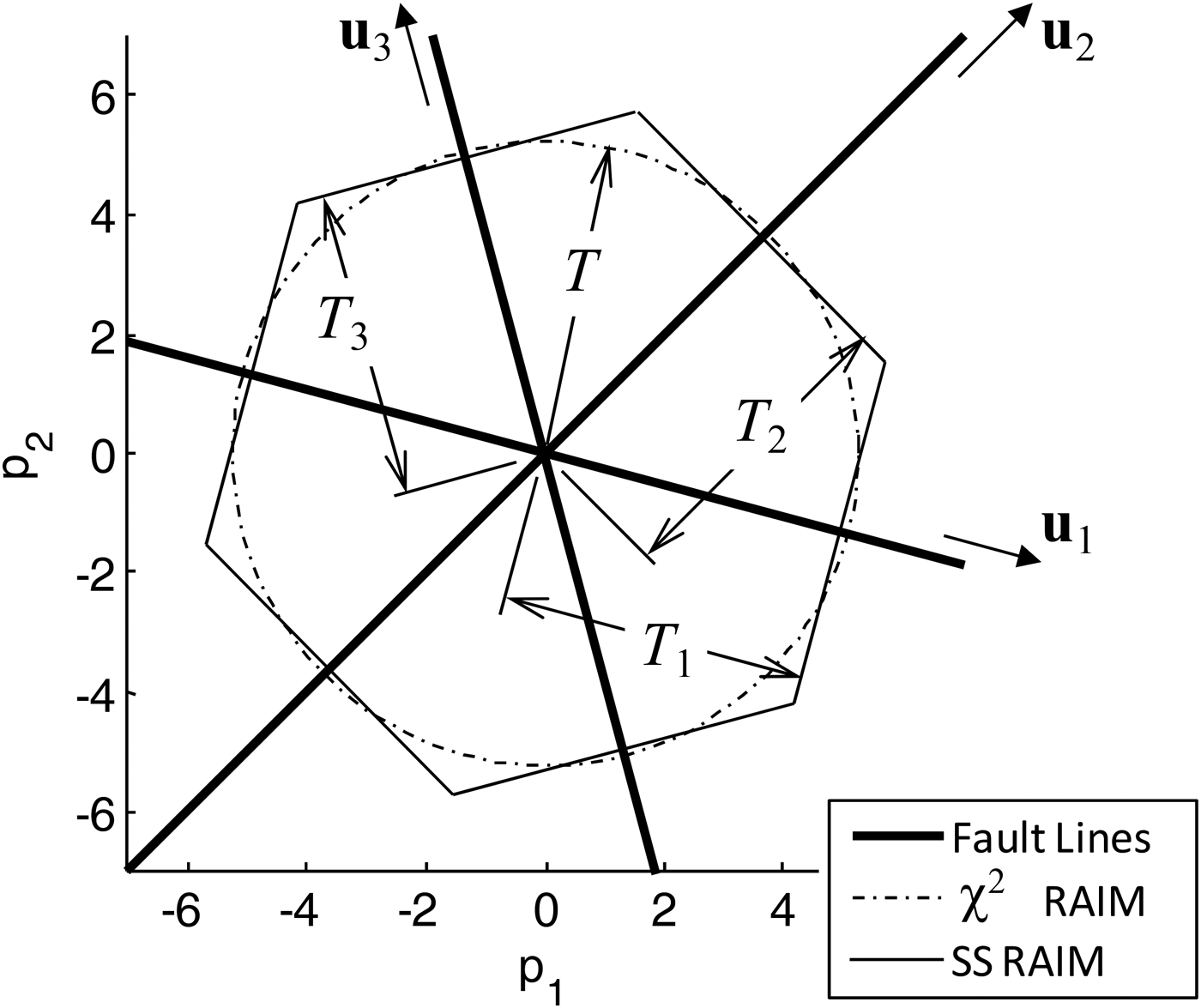
${\bf Q}{{\bf A}_i}$ is the i th column of Q. Vector ![]() ${{\bf u}_i}$ is the unit direction vector of the i th ‘fault mode line’, which can be represented in parity space (see Figure 1 in the next paragraphs) to visualise the noise-free impact on p of a fault on the i th measurement with magnitude varying from − ∞ to + ∞. Equation (27) expresses the fact that the n solution separations are projections of the parity vector on their corresponding fault mode lines.
${{\bf u}_i}$ is the unit direction vector of the i th ‘fault mode line’, which can be represented in parity space (see Figure 1 in the next paragraphs) to visualise the noise-free impact on p of a fault on the i th measurement with magnitude varying from − ∞ to + ∞. Equation (27) expresses the fact that the n solution separations are projections of the parity vector on their corresponding fault mode lines.
Equations (14) and (27) show that both q χ and q i are derived from the parity vector p. It has been proved in Joerger et al. (Reference Joerger, Chan and Pervan2014) that for any test statistic q lying in the parity space, the least-squares estimate error ε0 and q are statistically independent, so that the joint probability in Equation (6) can be expressed as:
The integrity risk bound obtained by substituting Equation (30) into Equation (6), and the result into Equation (2) is used in the remainder of this paper for both χ 2 and SS RAIM. This P HMI -bound differs from typical SS RAIM approaches (Brenner, Reference Brenner1996) because: (a) it does not use a position-domain-bound to account for the worst-case fault, and (b) it requires that the correlation between SS test statistics be evaluated in Section 3. A complete derivation of a conventional SS RAIM approach starting from Equation (1) can be found in Joerger et al. (Reference Joerger, Chan and Pervan2014). Based on this common definition for χ 2 and SS RAIM, differences in P HMI, or more precisely in probability of no-detection P(|q| <T | f i), can be displayed in parity space.
2.3. Parity Space Representations for an Illustrative Single-State Example
In this section, both χ 2 RAIM and SS RAIM are represented in parity space for an illustrative single-state example used in Potter and Suman (Reference Potter and Suman1977) and Joerger et al. (Reference Joerger, Chan and Pervan2014). Let us consider a scalar state x and a 3 × 1 measurement vector z that are expressed as:
where
Since m = 1 and n = 3, the (n − m) parity space is two-dimensional, which is convenient for display. The fault vector f represents three single-measurement faults, corresponding to three fault hypotheses H i, for i = 1, …, 3, with unknown fault magnitude f i.
 $${\bf f} = \left[ {\matrix{ {{\,f_1}} \cr 0 \cr 0 \cr}} \right]\quad {\rm or}\quad {\bf f} = \left[ {\matrix{ 0 \cr {{\,f_2}} \cr 0 \cr}} \right]\quad {\rm or}\quad {\bf f} = \left[ {\matrix{ 0 \cr 0 \cr {{\,f_3}} \cr}} \right]$$
Their three fault mode lines, with direction vectors ![]() ${{\bf u}_i}$ defined in Equation (28), are represented in Figure 1.
${{\bf u}_i}$ defined in Equation (28), are represented in Figure 1.

Figure 1. Detection boundaries for χ 2 (Circle) and SS (Hexagon) in parity space.
For χ 2 RAIM, the probability of no detection, which is the second term of the product in Equation (30), is given by: ![]() $P(q_\chi ^2 \lt T_\chi ^2 \vert {f_i})$. In contrast, for SS RAIM, the probability of no detection is a joint probability given by:
$P(q_\chi ^2 \lt T_\chi ^2 \vert {f_i})$. In contrast, for SS RAIM, the probability of no detection is a joint probability given by:
It follows from Equations (14), (27) and (34) that the detection boundaries for χ 2 and SS RAIM are a circle (or a hyper-sphere in higher-dimensional parity space) and a polygon (or a polytope), respectively.
Consistent with Equation (3), the SS detection thresholds can be computed using the following equation: ![]() $P\left( {\vert {q_1}\vert \ge {T_1} \cup \vert {q_2}\vert \ge {T_2} \cup \vert {q_3}\vert \ge {T_3}\vert {H_0}} \right) = {C_{REQ}}$ (where ‘
$P\left( {\vert {q_1}\vert \ge {T_1} \cup \vert {q_2}\vert \ge {T_2} \cup \vert {q_3}\vert \ge {T_3}\vert {H_0}} \right) = {C_{REQ}}$ (where ‘![]() $ \cup $’ captures a union of events, whereas commas in Equation (34) represent an intersection), for which a close approximation is given by:
$ \cup $’ captures a union of events, whereas commas in Equation (34) represent an intersection), for which a close approximation is given by:
 $${C_{REQ}} = \sum\limits_{i = 1}^h {{C_{REQ,i}}}, \quad {\rm e}{\rm. g}{\rm.,} \;{C_{REQ,i}} = \displaystyle{{{C_{REQ}}} \over n}$$
where the function Q −1{} is the inverse tail probability distribution of the two-tailed standard normal distribution (Q{} = 1 − Φ{}, where Φ{} is the standard normal cumulative distribution function).
Blanch et al. (Reference Blanch, Ene, Walter and Enge2007) suggests that for a practical application the difference is negligible between the probability of no detection for an optimised continuity risk requirement allocation versus the equal allocation expressed in Equation (36). In this example, because all three measurements contribute equally to estimation and detection, and because each fault occurrence is assumed equally likely (P H1 = P H2 = P H3), the optimal C REQ-allocation actually is the equal allocation in Equation (36). Following Equation (36), if the SS detection thresholds are all equal (T 1 = T 2 = T 3), then the polygon is a hexagon. In Figure 1, detection happens if the parity vector p lands outside the detection boundary. Therefore, the probability of no detection is the probability of being inside the dash-dotted circle for χ 2 RAIM, and inside the hexagon for SS RAIM.
Thus, χ 2 RAIM and SS RAIM each generate a different detection boundary, but it is unclear which one actually provides the highest probability of detection under a given fault hypothesis. Section 3 will show that the answer to this question depends on the navigation requirements ℓ and C REQ.
3. OPTIMAL PIECEWISE LINEAR DETECTION REGION IN RAIM
This section describes a method to establish the optimal piecewise linear detection region in RAIM. This optimisation method is used as an analytical tool to determine which of the χ 2 or SS test statistics gives the best detection capability, and under what circumstances.
3.1. Optimal Piecewise Linear Detection Boundary
Blanch et al. (Reference Blanch, Walter and Enge2013a) recently developed an approach, based on the Neyman-Pearson (NP) theorem, to visualize the optimal no-detection region by determining the set of points in parity space that contribute to reducing the integrity risk. This NP approach does not include a process to evaluate the integrity risk P HMI.
In contrast, in this section, a Piecewise Linear (PL) boundary is implemented to approximate the optimal detection region, which minimises the integrity risk. In this case, P HMI can be evaluated using an algorithm similar to SS RAIM, which is described below.
With regard to computation, the two approaches are intensive: the NP method involves sampling the parity space point by point, whereas the PL approximation determines a finite number of parameters based on the P HMI -bound defined in Section 2. The processing load for the PL approach can be reduced in future work using looser P HMI -bounds.
In this paper, the NP and PL algorithms are exploited to make an informed decision on whether to use χ 2 versus SS test statistics, depending on navigation requirements. The focus is on χ 2 and SS RAIM because these methods are computationally efficient and widely implemented.
The method's main idea for establishing the optimal detection boundary is illustrated in Figure 2 for the illustrative example described in Equations (31) to (33). To design a new detector, the method first uses the n SS test statistics (n = 3 in this case), which are projections of the parity vector p on the n fault lines (represented in grey). But the method also includes new test statistics, defined as projections of p onto lines selected at regular angular intervals (displayed in black), with unit direction vectors ![]() ${{\bf u}_4}$,
${{\bf u}_4}$, ![]() ${{\bf u}_5}$ and
${{\bf u}_5}$ and ![]() ${{\bf u}_6}$.
${{\bf u}_6}$.
As illustrated in Figure 1 with the hexagonal detection region for SS RAIM, each test statistic generates two segments of the piecewise linear boundary. Let d be the total number of detection test statistics. The higher d is, the finer the resolution of the detection boundary becomes. For clarity of exposition in the figures of this section, a total of d = 6 test statistics are considered, with detection thresholds T 1, …, T d.

Figure 2. Concept of Piecewise Linear Detection Region.
With this structure in place, finding the optimal detection boundary narrows down to determining the threshold values T 1, …, T d that minimise the integrity risk in Equation (2), while meeting the false alarm requirement in Equation (3). This problem can be formulated as a constrained minimisation problem:
 $$\mathop {\min} \limits_{{T_1}, \ldots, {T_d}} \left\{ {\sum\limits_{i = 0}^n {\mathop {\max} \limits_{{\,f_i}} P\left( { \vert {\varepsilon _0} \vert \gt \ell \vert {\,f_i}} \right)P\left( { \vert {q_1} \vert \lt {T_1}, \ldots, \vert {q_d} \vert \lt {T_d} \vert {\,f_i}} \right){P_{Hi}}}} \right\}$$
subject to: 1 − P(|q 1| <T 1, …, |q d| <T d | H 0)P H0 ≤ C REQ
The quantity to minimise is a bound on the integrity risk expressed in Equation (37) by substituting Equation (30) into Equation (6), and the result into Equation (2).
It is worth noting that the d test statistics q i are mutually correlated, so that the joint probability in Equation (37) cannot be written as a product of probabilities. Still, this joint probability can be numerically evaluated by stacking the test statistics q i in a d × 1 vector q. Let ![]() ${{\bf M}_U}$ be an (n − m) × d matrix such that
${{\bf M}_U}$ be an (n − m) × d matrix such that ![]() ${{\bf M}_U} = {\left[ {\matrix{ {{{\bf u}_1}} & \ldots & {{{\bf u}_d}} \cr}} \right]^T}$, and let
${{\bf M}_U} = {\left[ {\matrix{ {{{\bf u}_1}} & \ldots & {{{\bf u}_d}} \cr}} \right]^T}$, and let ![]() ${{\bf f}_i}$ be a n × 1 single-measurement fault vector whose only non-zero element is the ith element of value f i. The d × 1 vector of test statistics q follows a multivariate normal distribution with covariance matrix
${{\bf f}_i}$ be a n × 1 single-measurement fault vector whose only non-zero element is the ith element of value f i. The d × 1 vector of test statistics q follows a multivariate normal distribution with covariance matrix ![]() ${\bf M}_U^T {{\bf M}_U}$ and with mean vector
${\bf M}_U^T {{\bf M}_U}$ and with mean vector ![]() ${\bf M}_U^T {\bf Q}{{\bf f}_i}$ that can be evaluated given f i. In this case, the joint-probability evaluation is accomplished by integration over a hyper-box with edge lengths defined by the thresholds T i, for i = 1, …, d, following the methods in (Drezner and Wesolowsky, Reference Drezner and Wesolowsky1989) and (Genz and Bretz, Reference Genz and Bretz2002). As mentioned earlier, this multiple integration process is computationally expensive, and in this paper, is only used for analytical purposes in two illustrative examples.
${\bf M}_U^T {\bf Q}{{\bf f}_i}$ that can be evaluated given f i. In this case, the joint-probability evaluation is accomplished by integration over a hyper-box with edge lengths defined by the thresholds T i, for i = 1, …, d, following the methods in (Drezner and Wesolowsky, Reference Drezner and Wesolowsky1989) and (Genz and Bretz, Reference Genz and Bretz2002). As mentioned earlier, this multiple integration process is computationally expensive, and in this paper, is only used for analytical purposes in two illustrative examples.
Equation (37) describes the detection region as a union of half-planes, and is consistent with the assertion proved in Blanch et al. (Reference Blanch, Walter and Enge2013a), which states that the optimal detection boundary defines a closed, convex curve. Equation (37) is also written as a ‘mini-max’ problem. The maximisation is dealt with, in this paper, using a brute force approach based on multiple line-searches over f i, for i = 1, …, n. These line searches are repeated at each iteration of the minimisation process.
The problem formulation in Equation (37) can be modified into an unconstrained minimisation problem using the method of Lagrange multipliers (by forcing the inequality constraint to equality), or alternatively using barrier or penalty methods (Luenberger and Ye, Reference Luenberger and Ye2008). The first option is selected here, and Equation (37) becomes:
 $$\mathop {\min} \limits_{{T_1}, \ldots, {T_d},\theta} \left\{ \matrix{\sum\limits_{i = 0}^n {\mathop {\max} \limits_{{\,f_i}} P\left( { \vert {\varepsilon _0} \vert \gt \ell \vert {\,f_i}} \right)P\left( { \vert {q_1} \vert \lt {T_1}, \ldots, \vert {q_d} \vert \lt {T_d} \vert {\,f_i}} \right){P_{Hi}}} \hfill \cr + \theta \left[ {{C_{REQ}} - 1 + P\left( { \vert {q_1} \vert \lt {T_1}, \ldots, \vert {q_d} \vert \lt {T_d} \vert {H_0}} \right)} \right] \hfill} \right\}$$
where θ is the Lagrange multiplier, to be simultaneously determined with the optimal values of T i.
In Equation (38), the parameters to be optimised T 1, …, T d are limits of integration for the objective function. This facilitates the derivation in the Appendix, using the Leibniz integral rule, of analytical expressions for the objective function's gradient vector and Hessian matrix. An iterative Newton method can then be implemented to determine the optimal parameter values (Luenberger and Ye, Reference Luenberger and Ye2008). Convergence issues are beyond the scope of this paper since the optimisation method is not currently intended for practical implementation. The computational load of this piecewise-linear approximation will be readdressed in future work.
3.2. Sensitivity to Navigation Requirements
The optimal piecewise linear detection boundary is used here to make an educated choice between χ 2 RAIM and SS RAIM. The canonical example in Equations (31) to (33) is considered again, with the example parameter values: ![]() ${P_{{H_i}}} = {10^{ - 3}}$ for i = 1, …, 3, and C REQ = 10−3. The analysis is carried out for a range of values of the non-dimensional parameter ℓ/σ 0 (which is the ratio of the alert limit over the estimate error standard deviation).
${P_{{H_i}}} = {10^{ - 3}}$ for i = 1, …, 3, and C REQ = 10−3. The analysis is carried out for a range of values of the non-dimensional parameter ℓ/σ 0 (which is the ratio of the alert limit over the estimate error standard deviation).
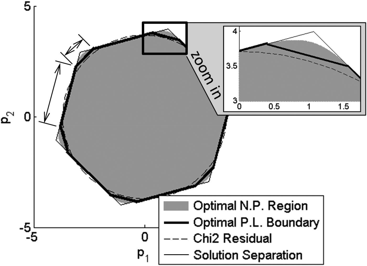
First, the optimal piecewise linear boundary is represented in Figure 3 (thick black lines) for a small value of ℓ/σ 0 (ℓ/σ 0 = 0.3). Segments of the optimal boundary are of equal length, so that the optimal boundary approaches a circle. This can be observed again in the zoomed-in window on the upper-right hand side of Figure 3, where the optimal boundary is close to the χ 2 circular boundary, and far from the corner of the SS hexagon.
This result is confirmed using the Neyman-Pearson (NP)-based approach (Blanch et al., Reference Blanch, Walter and Enge2013a), which, by sampling the parity space point by point, provides a precise depiction of the optimal no-detection region (grey area in Figure 3). In Figure 3, the optimal no-detection region closely matches the χ 2 RAIM circular boundary.
Thus, the χ 2 RAIM method approaches the optimal method for ℓ/σ 0 = 0.3. However, as ℓ/σ 0 increases, the optimal detection boundary changes. Figure 4 shows that for ℓ/σ 0 = 15, segments of the optimal piecewise linear boundary are no longer of equal length. The optimal region starts looking like a hexagon, which corresponds to the SS detection boundary. This can be seen again in the zoomed-in window where the optimal NP boundary starts filling in the corner of the SS hexagon.

Figure 3. Optimal Piecewise Linear (PL) detection boundary for ℓ/σ 0 = 0.3

Figure 4. Optimal Piecewise Linear (PL) detection boundary for ℓ/σ 0 = 15
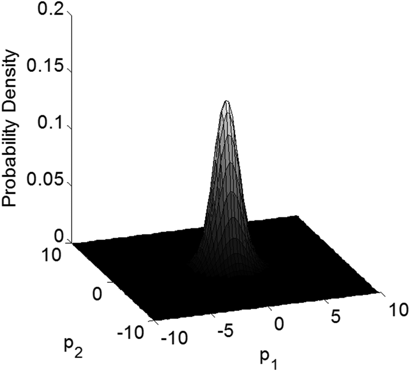
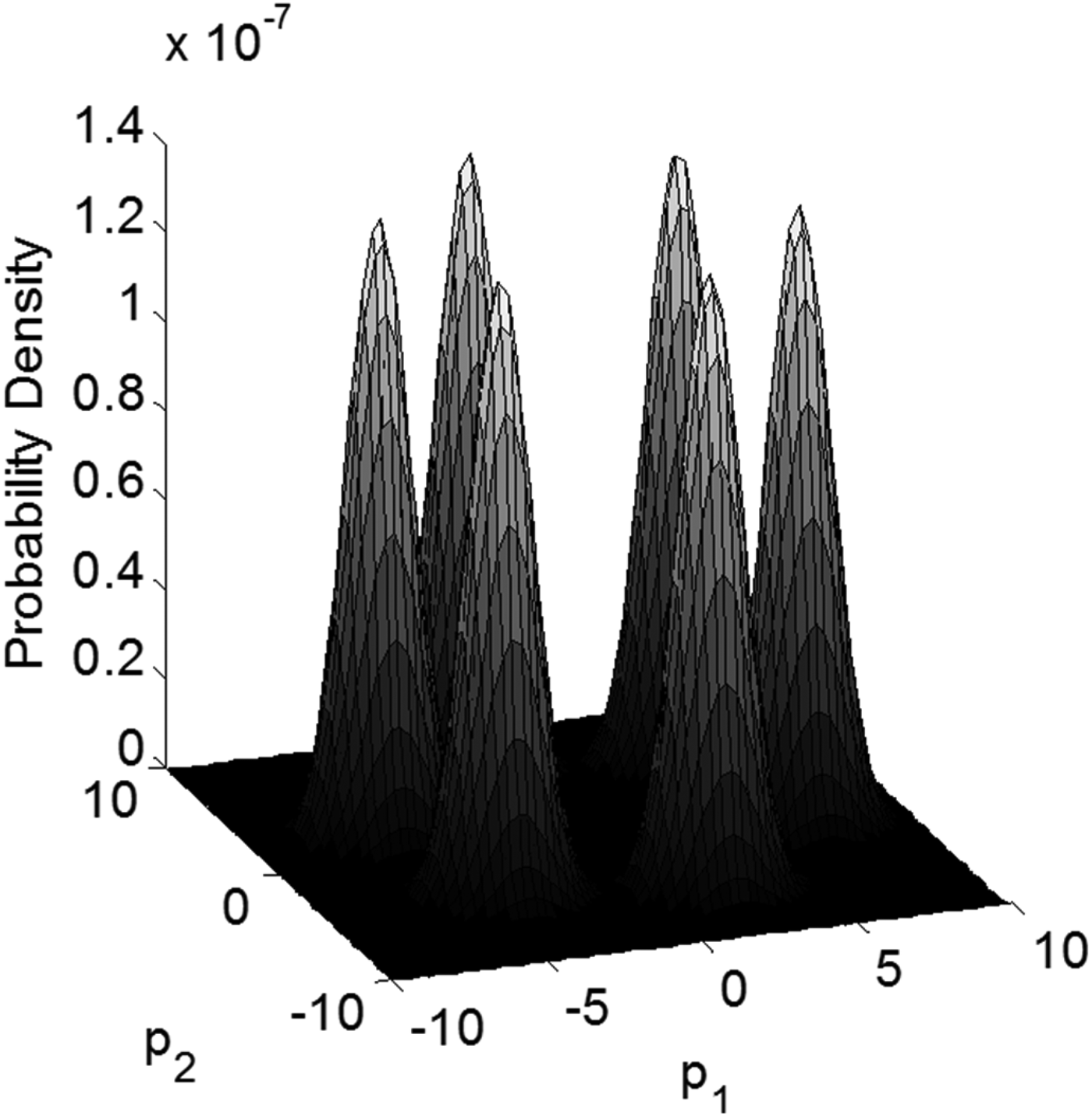
The next two paragraphs describe the dominating factors causing the optimal detection region to change with ℓ/σ 0. First, the constraint in the problem statement of Equation (37) is independent of ℓ/σ 0. Thus the optimal area is only shaped by the objective function, i.e., by the integrity risk P HMI, which is a sum of probabilities over multiple hypotheses. The probability density function for P HMI is represented in parity space for ℓ/σ 0 = 0.3 and ℓ/σ 0 = 15 in Figures 5 and 6, respectively. In this multiple hypothesis formulation, the density function is a composite of seven peaks of probability density, corresponding to the fault-free hypothesis H 0, and to the three fault hypotheses for positive and negative values of the fault magnitude. The continuity risk requirement defines an area near the origin corresponding to relatively small fault magnitudes, which are difficult to detect.
Figure 5 shows what appears to be a single peak in probability density for small values of ℓ/σ 0. When ℓ/σ 0 is small, the probability of the estimate error ε0 exceeding ℓ rises rapidly, even for small, difficult-to-detect fault magnitudes. It follows that the worst-case fault magnitudes (which maximise P HMI) remain close to zero, and the seven peaks are all brought together near the origin. In contrast, as ℓ/σ 0 increases in Figure 6, small-magnitude faults do not cause hazardous information so that the worst-case fault magnitudes become larger, and the six probability density peaks corresponding to fault hypotheses spread apart along the fault mode lines. Therefore, as ℓ/σ 0 increases, the optimal detection boundary changes from a circular area (χ 2) to a polygon (SS).

Figure 5. Density function of the probability of HMI for ℓ/σ 0 = 0.3

Figure 6. Density function of the probability of HMI for ℓ/σ 0 = 15
In practice, the alert limit ℓ must be substantially greater than σ 0 or the fault-free integrity risk alone (i.e., the term of the sum in Equation (2) for which i = 0) will exceed the integrity risk requirement I REQ. Moreover, comparing the scales of the z-axes in Figures 5 and 6 provides a clue as to the difference in orders of magnitude of P HMI as ℓ/σ 0 changes. Therefore for most realistic practical requirements (i.e., for large values of ℓ/σ 0), the optimal detection boundary approaches SS. This result completes and reinforces the findings of previous papers (Joerger et al., Reference Joerger, Chan and Pervan2014; Blanch et al., Reference Blanch, Walter and Enge2013a).
3.3. Optimal detection boundary for an Example GPS Satellite Geometry
In this section, the optimal NP and PL boundaries are derived for the example GPS satellite geometry displayed in Figure 7. In this case, the state vector x in Equation (4) comprises three position coordinates and one receiver clock bias. Since the number of satellite measurements n is six, and the number of states m is four, the parity space has dimension (n − m) = 2. Example parameter values are the same as in Section 3.2: ![]() ${P_{{H_i}}} = {10^{ - 3}}$ for i = 1, …, 3, and C REQ = 10−3.
${P_{{H_i}}} = {10^{ - 3}}$ for i = 1, …, 3, and C REQ = 10−3.
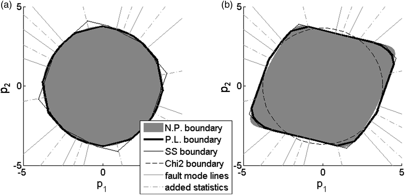
Figure 8 shows the optimal detection boundaries for ℓ/σ 0 = 10−4, and for ℓ/σ 0 = 7. In both cases, the ‘SS boundary’ is displayed for the optimal C REQ-allocation, which, in this example, is no longer the equal allocation. The optimal allocation and the corresponding detection thresholds are found by solving Equation (38) for the six SS RAIM test statistics. In practical applications, optimal allocation does not cause large P HMI -reductions as compared to equal allocation (Blanch et al., Reference Blanch, Ene, Walter and Enge2007), but it does in this particular example.
In parallel, the optimal PL boundary is defined using the six SS test statistics, with parity space directions the solid grey lines in Figure 8 (along vectors ![]() ${{\bf u}_i}$, for i = 1, …, 6) as well as six additional statistics, determined by projecting the parity vector on the grey dash-dotted lines (for example, along vectors
${{\bf u}_i}$, for i = 1, …, 6) as well as six additional statistics, determined by projecting the parity vector on the grey dash-dotted lines (for example, along vectors ![]() ${{\bf u}_{i + 6}} = \left( {{{\bf u}_i} + {{\bf u}_{i + 1}}} \right)/\vert\vert {{\bf u}_i} + {{\bf u}_{i + 1}}\vert\vert$ for i = 1, …, 5, and
${{\bf u}_{i + 6}} = \left( {{{\bf u}_i} + {{\bf u}_{i + 1}}} \right)/\vert\vert {{\bf u}_i} + {{\bf u}_{i + 1}}\vert\vert$ for i = 1, …, 5, and ![]() ${{\bf u}_{12}} = \left( {{{\bf u}_1} + {{\bf u}_6}} \right)/\vert\vert {{\bf u}_1} + {{\bf u}_6}\vert\vert$). These lines are placed right in-between fault lines to accentuate their impact on the detection boundary as compared to SS RAIM.
${{\bf u}_{12}} = \left( {{{\bf u}_1} + {{\bf u}_6}} \right)/\vert\vert {{\bf u}_1} + {{\bf u}_6}\vert\vert$). These lines are placed right in-between fault lines to accentuate their impact on the detection boundary as compared to SS RAIM.
For example, in Figure 8(a), the optimal NP and PL boundaries expectedly match the circle corresponding to the χ 2 circle (as explained in Section 3.2). The SS boundary does not match the circle quite as well, especially considering the corners of the SS polygon where the angular separation between fault lines is largest.
However in Figure 8(b) the optimal NP, PL, and SS boundaries are no longer circular. All three approaches provide fairly consistent boundaries, except for small differences at the corners of the polygon, where probability densities under H 0 become extremely small. The PL method enables evaluation of the integrity risk P HMI. Let P HMI,χ be the integrity risk derived from χ 2 RAIM. In this example, the integrity risk is reduced to 0·92 P HMI,χ for SS RAIM versus 0·91 P HMI,χ using the PL method. In this case, the SS RAIM integrity performance approaches that of the optimal PL method.
In Part 2 of this work (Joerger et al., Reference Joerger, Langel and Pervan2015), the Least-Squares (LS) solution separation (SS) detection test statistics are used as a starting point, because they provide a computationally-efficient, practical approximation of the optimal detection region when using a LS estimator.

Figure 7. Azimuth-elevation sky plot for an example GPS satellite geometry.

Figure 8. Optimal Piecewise Linear (PL) detection boundary for the example GPS satellite geometry in Figure 7, (a) for ℓ/σ 0 = 10−4, and (b) for ℓ/σ 0 = 7
4. CONCLUSION
This paper is Part 1 of a two-part research effort, which presents new methods to minimise the integrity risk by design of the RAIM detector and estimator for applications in future multi-constellation GNSS-based navigation.
In this paper, a piecewise linear approximation of the optimal detection region in parity space was established. Unlike previously published approaches, this optimisation method enables integrity risk evaluation, but would require significant refinement in future work for real time implementations.
However, the method is immediately useful in that it provides a means to determine, for example scenarios, which of Solution Separation (SS) or chi-squared (χ 2) RAIM yields the lowest integrity risk. The focus is placed on these two algorithms because they are computationally efficient and widely implemented. The paper shows, with the aid of two example measurement equations, that the optimal detection region varies with navigation system parameters, and that for realistic requirements, the SS detection region can approach the optimal boundary. Therefore, the new RAIM methods in Part 2 of this work will be devised using SS test statistics.
Part 2 of this research in Joerger et al. (Reference Joerger, Langel and Pervan2015) will investigate the potential of reducing the integrity risk using a Non-Least-Squares (NLS) estimator. In addition, performance analyses will be carried out to evaluate the new RAIM method, using the SS detector and NLS estimator, for an example aircraft approach applications using multi-constellation Advanced RAIM.
ACKNOWLEDGMENTS
The authors would like to thank the Federal Aviation Administration for sponsoring this work.
APPENDIX. GRADIENT AND HESSIAN DERIVATION FOR THE OPTIMAL DETECTOR
The derivation of the optimal piecewise linear detection region in parity space was formulated as a constrained minimisation problem over detection thresholds T 1, …, T d in Equation (37). This Appendix provides the main steps of the gradient vector and Hessian matrix derivation, which allows us to efficiently solve Equation (37) using Newton's method.
The integrity risk, i.e., the objective function in Equation (37), can be bounded using the following inequality:
 $$\eqalign{& \sum\limits_{i = 0}^h {P\left( { \vert {\varepsilon _0} \vert \gt \ell, \vert {q_1} \vert \lt {T_1}, \ldots, \vert {q_d} \vert \lt {T_d} \vert {\,f_i}} \right){P_{Hi}}} \cr & \le P\left( { \vert {\varepsilon _0} \vert \gt \ell, \vert {H_0}} \right){P_{H0}} + \sum\limits_{i = 1}^h {{a_i}P\left( { \vert {q_1} \vert \lt {T_1}, \ldots, \vert {q_d} \vert \lt {T_d} \vert {\,f_i}} \right)}} $$
where
and where, to lighten the notation, the maximum over f i is not expressed. Equation (A1) uses the fact proved in Joerger et al. (Reference Joerger, Chan and Pervan2014) that ε0 and q i, for i = 1, …, d, are statistically independent. The coefficient a i and the term corresponding to the fault-free hypothesis H 0 on the right hand side of Equation (A1) are independent of the detection thresholds. The minimisation problem over thresholds T 1, …, T d can therefore be rewritten as:
 $$\mathop {\min} \limits_{{T_1}, \ldots, {T_d}} \left\{ {\sum\limits_{i = 1}^h {{a_i}P\left( { \vert {q_1} \vert \lt {T_1}, \ldots, \vert {q_d} \vert \lt {T_d} \vert {\,f_i}} \right)}} \right\}$$
subject to:
The terms that are a function of the thresholds T i are the joint probabilities of |q j| <T j for j = 1, …, d, given ![]() ${\bar{\bf f}_i}$ for i = 1, …, h in the objective function in Equation (A3), and given H 0 in the constraint Equation (A4). These terms appear in a sum after modifying the problem formulation in Equations (A3) and (A4) into an unconstrained minimisation problem, e.g., using the method of Lagrange multipliers given in Equation (38). For clarity of exposition, we consider a simplified objective function ψ (for d = 3), which lets us capture the main steps of the derivation for the modified objective function in Equation (38) (the derivation is extendible to arbitrary d). ψ is defined as:
${\bar{\bf f}_i}$ for i = 1, …, h in the objective function in Equation (A3), and given H 0 in the constraint Equation (A4). These terms appear in a sum after modifying the problem formulation in Equations (A3) and (A4) into an unconstrained minimisation problem, e.g., using the method of Lagrange multipliers given in Equation (38). For clarity of exposition, we consider a simplified objective function ψ (for d = 3), which lets us capture the main steps of the derivation for the modified objective function in Equation (38) (the derivation is extendible to arbitrary d). ψ is defined as:
 $$\eqalign{\psi \left( {{T_1},{T_2},{T_3}} \right) \equiv & P\left( { \vert {q_1} \vert \lt {T_1}, \vert {q_2} \vert \lt {T_2}, \vert {q_3} \vert \lt {T_3}} \right) \cr = & \int\limits_{ - {T_3}}^{{T_3}} {\int\limits_{ - {T_2}}^{{T_2}} {\int\limits_{ - {T_1}}^{{T_1}} {\phi ({q_1},{q_2},{q_3})} d{q_1}d}} {q_2}d{q_3}} $$
where q 1, q 2, and q 3 are correlated random variables, and ϕ() is the probability density function for a non-zero mean multivariate normal distribution. The following derivation applies in the special case where variables q 1, q 2, and q 3 have zero mean, as is the case in the constraint Equation (A4).
For the minimisation problem over detection thresholds T 1, T 2, T 3, the first element of the gradient vector can be expressed, using the Leibniz integral rule, as:
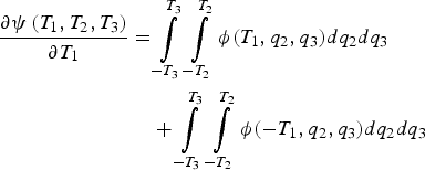 $$\eqalign{\displaystyle{{\partial \psi \left( {{T_1},{T_2},{T_3}} \right)} \over {\partial {T_1}}} =& \int\limits_{ - {T_3}}^{{T_3}} {\int\limits_{ - {T_2}}^{{T_2}} {\phi ({T_1},{q_2},{q_3})d}} {q_2}d{q_3} \cr& + \int\limits_{ - {T_3}}^{{T_3}} {\int\limits_{ - {T_2}}^{{T_2}} {\phi ( - {T_1},{q_2},{q_3})d}} {q_2}d{q_3}} $$
The expression in Equation (A6) cannot easily be evaluated because q 1, q 2, and q 3 are correlated. Let ζ be an infinitesimally small number. Equation (A6) can be rewritten and approximated as:
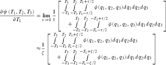 $$\eqalign{\displaystyle{{\partial \psi \left( {{T_1},{T_2},{T_3}} \right)} \over {\partial {T_1}}} = & \mathop {\lim} \limits_{\tau \to 0} \displaystyle{1 \over \tau} \left[ \matrix{\int\limits_{ - {T_3}}^{{T_3}} {\int\limits_{ - {T_2}}^{{T_2}} {\int\limits_{{T_1} - \tau /2}^{{T_1} + \tau /2} \phi ({q_1},{q_2},{q_3})d{q_1}d}} {q_2}d{q_3} \hfill \cr \quad + \int\limits_{ - {T_3}}^{{T_3}} {\int\limits_{ - {T_2}}^{{T_2}} {\int\limits_{ - {T_1} - \tau /2}^{ - {T_1} + \tau /2} {\phi ({q_1},{q_2},{q_3})} d{q_1}d}} {q_2}d{q_3} \hfill} \right] \cr \approx & \displaystyle{1 \over \zeta} \left[ \matrix{\int\limits_{ - {T_3}}^{{T_3}} {\int\limits_{ - {T_2}}^{{T_2}} {\int\limits_{{T_1} - \zeta /2}^{{T_1} + \zeta /2} \phi ({q_1},{q_2},{q_3})d{q_1}d}} {q_2}d{q_3} \hfill \cr \quad + \int\limits_{ - {T_3}}^{{T_3}} {\int\limits_{ - {T_2}}^{{T_2}} {\int\limits_{ - {T_1} - \zeta /2}^{ - {T_1} + \zeta /2} {\phi ({q_1},{q_2},{q_3})} d{q_1}d}} {q_2}d{q_3} \hfill} \right]} $$
The above expression enables the use of existing numerical methods (Drezner and Wesolowsky, Reference Drezner and Wesolowsky1989) to evaluate the right hand side term in Equation (A7), by integration of the tri-variate normally distributed random vector ![]() ${\left[ {\matrix{ {{q_1}} & {{q_2}} & {{q_3}} \cr}} \right]^T}$ over a box. The second and third elements of the 3 × 1 gradient vector are obtained in the same manner as in Equation (A7), by taking the partial derivatives of ψ( ) over T 2, and T 3, respectively.
${\left[ {\matrix{ {{q_1}} & {{q_2}} & {{q_3}} \cr}} \right]^T}$ over a box. The second and third elements of the 3 × 1 gradient vector are obtained in the same manner as in Equation (A7), by taking the partial derivatives of ψ( ) over T 2, and T 3, respectively.
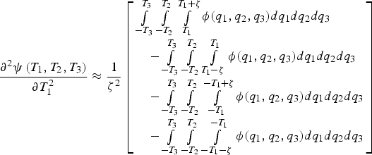
The same method is used to determine the off-diagonal and diagonal elements of the Hessian matrix, which are respectively expressed as:
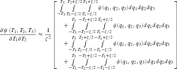 $$\displaystyle{{\partial \psi \left( {{T_1},{T_2},{T_3}} \right)} \over {\partial {T_1}\partial {T_2}}} \approx \displaystyle{1 \over {{\zeta ^2}}}\left[ \matrix{\int\limits_{ - {T_3}}^{{T_3}} {\int\limits_{{T_2} - \zeta /2}^{{T_2} + \zeta /2} {\int\limits_{{T_1} - \zeta /2}^{{T_1} + \zeta /2} \phi ({q_1},{q_2},{q_3})d{q_1}d}} {q_2}d{q_3} \hfill \cr \quad + \int\limits_{ - {T_3}}^{{T_3}} {\int\limits_{ - {T_2} - \zeta /2}^{ - {T_2} + \zeta /2} {\int\limits_{{T_1} - \zeta /2}^{{T_1} + \zeta /2} {\phi ({q_1},{q_2},{q_3})} d{q_1}d}} {q_2}d{q_3} \hfill \cr \quad + \int\limits_{ - {T_3}}^{{T_3}} {\int\limits_{{T_2} - \zeta /2}^{{T_2} + \zeta /2} {\int\limits_{ - {T_1} - \zeta /2}^{ - {T_1} + \zeta /2} {\phi ({q_1},{q_2},{q_3})} d{q_1}d}} {q_2}d{q_3} \hfill \cr \quad + \int\limits_{ - {T_3}}^{{T_3}} {\int\limits_{ - {T_2} - \zeta /2}^{ - {T_2} + \zeta /2} {\int\limits_{ - {T_1} - \zeta /2}^{ - {T_1} + \zeta /2} {\phi ({q_1},{q_2},{q_3})} d{q_1}d}} {q_2}d{q_3} \hfill} \right]$$
 $$\displaystyle{{{\partial ^2}\psi \left( {{T_1},{T_2},{T_3}} \right)} \over {\partial T_1^2}} \approx \displaystyle{1 \over {{\zeta ^2}}}\left[ \matrix{\int\limits_{ - {T_3}}^{{T_3}} {\int\limits_{ - {T_2}}^{{T_2}} {\int\limits_{{T_1}}^{{T_1} + \zeta} \phi ({q_1},{q_2},{q_3})d{q_1}d}} {q_2}d{q_3} \hfill \cr \quad - \int\limits_{ - {T_3}}^{{T_3}} {\int\limits_{ - {T_2}}^{{T_2}} {\int\limits_{{T_1} - \zeta} ^{{T_1}} {\phi ({q_1},{q_2},{q_3})} d{q_1}d}} {q_2}d{q_3} \hfill \cr \quad - \int\limits_{ - {T_3}}^{{T_3}} {\int\limits_{ - {T_2}}^{{T_2}} {\int\limits_{ - {T_1}}^{ - {T_1} + \zeta} {\phi ({q_1},{q_2},{q_3})} d{q_1}d}} {q_2}d{q_3} \hfill \cr \quad - \int\limits_{ - {T_3}}^{{T_3}} {\int\limits_{ - {T_2}}^{{T_2}} {\int\limits_{ - {T_1} - \zeta} ^{ - {T_1}} {\phi ({q_1},{q_2},{q_3})} d{q_1}d}} {q_2}d{q_3} \hfill} \right]$$
Equations (A7) to (A9) provide the main results needed to determine the gradient vector and Hessian matrix of the modified objective function in Equation (38).


