


1. Introduction
In recent years, significant advances have been made in radio astronomy. The Square Kilometre Array (SKA, Dewdney et al. Reference Dewdney, Hall, Schilizzi and Lazio2009), the world’s largest radio telescope currently under construction, is expected to deliver groundbreaking discoveries while addressing the challenge of handling the vast amounts of data it will generate. Meanwhile, many exciting scientific endeavours, such as understanding the cosmic dawn (CD) and the epoch of reionisation (EoR) by observing the ultra-faint neutral hydrogen redshifted 21-cm line signal at low frequencies, will require exceptionally high-quality data, minimising radio frequency interferenc (RFI) (Fridman & Baan Reference Fridman and Baan2001; Offringa et al. Reference Offringa, de Bruyn, Zaroubi and Biehl2010) as much as possible. There is evidence suggesting that even fainter RFIs in Murchison Widefield Array (MWA, Tingay et al. Reference Tingay2013) data are likely to contaminate the EoR power spectrum (Wilensky et al. Reference Wilensky2023). The need for larger and higher-quality datasets drives the development of automatic RFI mitigation methods to reduce the manual burden and increase the efficiency and precision of the results.
Generally, RFI is different from celestial radio signals, which will contaminate the astronomical data and severely affect the observation results of radio telescopes (Fridman & Baan Reference Fridman and Baan2001). The sources of RFI are diverse, including radio broadcasts (Huang et al. Reference Huang, Wu, Zheng, Gu and Xu2016), digital television (DTV, Wilensky et al. Reference Wilensky, Morales, Hazelton, Barry, Byrne and Roy2019), satellites (Sokołowski et al. 2015), meteor trails (Zhao et al. Reference Zhao, Liang, Yang, Shan, Zheng, Zhang and Guo2023), lightning (Sokołowski et al. 2015), aircraft communication (Gehlot et al. Reference Gehlot2023), and internal sources such as computers and screens (Porko et al. Reference Porko2011). Due to the continuous expansion of human activities and the rapid development of radio technology, radio telescopes are facing an increasing amount of RFI. Mitigating the RFI has become increasingly challenging. With the deluge of big data from new radio telescopes coming into operation and the need for high-quality data, the mitigation of RFI must be considered a pressing and crucial issue that must be addressed (Anstey & Leeney Reference Anstey and Leeney2023).
The complex temporal and frequency structures of RFI make it challenging to model and obtain a universal method of RFI mitigation (Fridman & Baan Reference Fridman and Baan2001). In fact, many different methods have been proposed and adopted based on specific circumstances. In the proactive mitigation stage, there are approaches such as establishing a radio quiet zone (RQZ, Wang et al. Reference Wang2023), setting up protected frequency bands (Furlanetto, Peng Oh, & Briggs Reference Furlanetto, Peng Oh and Briggs2006), choosing locations with topographical features such as mountains (Klein Wolt et al. Reference Klein Wolt, Aminaei, Zarka, Schrader, Boonstra and Falcke2012), and using multi-layer electromagnetic shielding (Wang et al. Reference Wang2023; Ambrosini et al. Reference Ambrosini, Bolli, Bortolotti, Gaudiomonte, Messina and Roma2009). It is still necessary to adopt reactive mitigation methods in subsequent steps. Offringa et al. (Reference Offringa, de Bruyn, Zaroubi and Biehl2010) proposed a combinatorial threshold algorithm: the SumThreshold method. AOFlagger, developed based on this threshold method, has been applied in Low Frequency Array (LOFAR) and MWA (Offringa, van de Gronde, & Roerdink Reference Offringa, van de Gronde and Roerdink2012; Offringa et al. Reference Offringa2015). Wilensky et al. (Reference Wilensky, Morales, Hazelton, Barry, Byrne and Roy2019) introduced a new method called Sky-Subtracted Incoherent Noise Spectra (SSINS), and its effectiveness was demonstrated by applying it to several kinds of RFI identified in data from MWA. For the 21 CentiMeter Array (21CMA), time-varying RFI is mitigated by handling weighted visibilities (Huang et al. Reference Huang, Wu, Zheng, Gu and Xu2016; An et al. Reference An, Chen, Mohan and Lao2017).
With rapid advancements in machine learning and deep learning, an increasing number of studies are applying machine learning to the field of astronomy in the face of vast observational data. In research on the mitigation of RFI, a large number of models based on deep learning have been used to detect RFI. Haomin et al. (Reference Haomin, Deng, Wang, Mei, Xu, Smirnov, Deng and Wei2022) proposed a model using the convolutional neural network (CNN) to identify RFI. Akeret et al. (Reference Akeret, Chang, Lucchi and Refregier2016) successfully developed the U-Net in the field of RFI detection. To address the frequent errors encountered when CNN is used for the RFI flagging of FAST data, RFI-net was developed (Yang et al. Reference Yang, Yu, Xiao and Zhang2020). The mask region-based convolutional neural network (mask R-CNN) has been integrated with point-based rendering (PointRend) to identify RFI when finding HI galaxies (Liang et al. Reference Liang2023).
Compared with traditional methods that require manual intervention to specify algorithm parameters, deep learning greatly improves the efficiency of data processing. However, it also has certain limitations. Model training, for instance, requires that a large amount of RFI data to be prepared as a training set, which is a burden. Using simulated RFI data to train models is a common choice. However, considering that real-world RFIs are often much more complex than mock data, models trained on simple simulated RFI may not perform optimally for complicated RFI recognition (Yang et al. Reference Yang, Yu, Xiao and Zhang2020). Additionally, there is a risk that the model may become dependent on training data or overfit, leading to missed detections of unknown RFI. Existing models are usually designed for specific tasks or telescopes and often lack sufficient generalisation capability, making them cumbersome to use for other applications.The same issues arise in other fields where deep learning is applied, such as solar radio burst (SRB) detection and the search for pulsars or FRBs. These applications also suffer from problems like too few samples to build a training set and data imbalance (Guo et al. Reference Guo, Wan, Hu, Wang and Yan2022; Liu et al. Reference Liu, Lao, An, Xu and Zhang2021). Thus, we wonder if it is possible to develop a method based on an open-source model with strong generalisation capability that researchers from various fields can use directly with minimal fine-tuning or structural adjustment. This approach would not only reduce the burden of designing and training models from scratch but also minimise the drawbacks associated with model training, while hopefully retaining the ability to identify unknown events.
Kirillov et al. (Reference Kirillov2023) proposed a model called the Segment Anything Model (SAM) for image recognition and segmentation. They utilised model-in-the-loop dataset annotation to construct the largest segmentation dataset to date, containing over 1 billion masks on 11 million images, for training. This approach gave SAM powerful generalisation and zero-shot capability, which has been proven by its application in various fields (Yu et al. Reference Yu, Feng, Feng, Liu, Jin, Zeng and Chen2023; Shen et al. Reference Shen, Yang and Wang2023). HQ-SAM builds on SAM by adding a High-Quality Output Token to improve the quality of the predicted masks while preserving SAM’s generalisation capability (Ke et al. Reference Ke, Ye, Danelljan, Liu, Tai, Tang and Yu2023). Inspired by the impressive generalisation capability and ease of use of HQ-SAM (SAM), in this paper, we apply it to the field of radio astronomy. We explore its performance in RFI or events detection such as SRB, demonstrating the model’s good generalisation capability and recognition ability in this domain. By using the HQ-SAM (SAM) model, along with minor fine-tuning and modifications, we hope to find a better solution to the aforementioned challenges.
The structure of this paper is as follows. Section 2 introduces SAM, HQ-SAM, and the SumThreshold method, which we use for comparison with the first two in detail. Section 3 shows the real RFI from the 21CMA and the detection results using the three methods. Section 4 demonstrates the recognition results of our mock RFI. Section 5 applies HQ-SAM to the search for SRB. We discuss our findings in Section 6 and provide our conclusions in Section 7.
2. Method
In this section, we will introduce several methods and techniques used in subsequent research, including SAM, HQ-SAM, and the SumThreshold method.
2.1 Segment Anything Model (SAM) and HQ-SAM
The Segment Anything Model is a groundbreaking image recognition and segmentation model capable of generating valid segmentation masks when provided with any form of segmentation prompt (points, box, mask, text, etc.). SAM consists of three components: an image encoder, a prompt encoder, and a lightweight mask decoder that combines the information from the first two to predict segmentation masks (Kirillov et al. Reference Kirillov2023). When using SAM, one simply needs to provide prompts indicating the content to be segmented in the image. SAM offers an automatic segmentation mode that evenly distributes points on the segmentation image to act as point prompts. The output will include multiple masks due to SAM’s ambiguity-aware feature. Because the researchers built a massive segmentation dataset named SA-1B, containing over 1 billion masks and 11 million images to train the model, SAM has strong zero-shot capability (meaning the model can successfully identify or segment objects it has never specifically been trained on) and demonstrates outstanding performance across many tasks.
Due to the impressive zero-shot and generalisation capability of SAM, it has been applied to a wide range of fields. Ma et al. (Reference Ma, He, Li, Han, You and Wang2024) proposed MedSAM by fine-tuning SAM with a medical image training dataset, demonstrating that this model can produce accurate segmentation in various medical image segmentation tasks. RSPrompter (Chen et al. Reference Chen, Liu, Chen, Zhang, Li, Zou and Shi2023) is a method that creates appropriate prompts for SAM, enabling SAM to perform well in instance segmentation tasks for remote sensing images. Nguyen, Phung, & Cao (Reference Nguyen, Phung and Cao2023) utilised two pre-trained object detection models, You Only Look Once (YOLO)-v8 and DETR with Improved deNoising anchOr boxes (DINO), to first detect objects in the image and then used the detected bounding boxes as box prompts for SAM. This approach allowed SAM to achieve good scores in panoptic segmentation tasks for weeds and crops.
Although SAM has shown promising results in various fields, there are still some limitations in its application. SAM cannot automatically interpret images from different domains to generate appropriate prompts for itself or provide semantic categories for the predicted masks (Liu et al. Reference Liu, Zhu, Li, Chen, Wang and Shen2024). As a result, many works design additional components to automatically generate suitable prompts when applying SAM, such as Chen et al. (Reference Chen, Liu, Chen, Zhang, Li, Zou and Shi2023) and Nguyen et al. (Reference Nguyen, Phung and Cao2023), which were mentioned earlier. Additionally, SAM exhibits certain shortcomings when dealing with targets featuring complex background interference, ambiguous boundaries, or low image contrast (Wu et al. Reference Wu, Ji, Liu, Fu, Xu, Xu and Jin2023).
Ke et al. (Reference Ke, Ye, Danelljan, Liu, Tai, Tang and Yu2023) identified two key issues with the segmentation results of SAM in some cases: coarse mask boundaries and incorrect predictions, which can significantly affect SAM’s applicability and effectiveness. To address these problems, they proposed an upgraded model called HQ-SAM.Footnote a HQ-SAM enhances the quality of predicted masks by incorporating a learnable High-Quality Output Token into SAM’s mask decoder. This method allows HQ-SAM to retain the pre-trained model weights of SAM, thus preserving SAM’s original zero-shot capability, while also enabling more precise segmentation across various tasks.
Overall, there is no significant difference between running HQ-SAM and SAM. SAM resizes input images of any size to 1 024
 $\times$
1 024 pixels, meaning that smaller images will be enlarged more, which facilities better features extraction by the model. However, there is a potential risk of image quality loss with this enlargement, so it is important to ensure the clarity and detail of the input images. Considering the above points, users need to select the size best suited to their specific task. In automatic segmentation mode, SAM provides several adjustable parameters to optimise performance. For example, the parameter
$\times$
1 024 pixels, meaning that smaller images will be enlarged more, which facilities better features extraction by the model. However, there is a potential risk of image quality loss with this enlargement, so it is important to ensure the clarity and detail of the input images. Considering the above points, users need to select the size best suited to their specific task. In automatic segmentation mode, SAM provides several adjustable parameters to optimise performance. For example, the parameter
 $points\_per\_side$
determines the number of sampling points along one side of the image, with the total number of points being
$points\_per\_side$
determines the number of sampling points along one side of the image, with the total number of points being
 $points\_per\_side^2$
. Generally, increasing the number of sampling points improves recognition accuracy but also demands longer processing times, necessitating a trade-off. For more details on these parameters, please refer to SAM’s documentation.Footnote
b
$points\_per\_side^2$
. Generally, increasing the number of sampling points improves recognition accuracy but also demands longer processing times, necessitating a trade-off. For more details on these parameters, please refer to SAM’s documentation.Footnote
b
In this work, our primary focus is on applying SAM (HQ-SAM) to astronomical research areas including RFI and SRB, where deep learning techniques can offer significant benefits. We aim to assess whether we can achieve a broadly applicable model in astronomy with minimal cost (i.e. without extensive fine-tuning or structural modifications) while mitigating common issues associated with model training. To this end, we utilise the automatic segmentation mode provided by SAM, employing the same parameters for both SAM and HQ-SAM. Except for images of SRBs, which are sized at 1 225
 $\times$
645 pixels, all other images are standardised to 200
$\times$
645 pixels, all other images are standardised to 200
 $\times$
200 pixels so that it will be enlarged by about 25 times, allowing for better recognition results.
$\times$
200 pixels so that it will be enlarged by about 25 times, allowing for better recognition results.
2.2 The SumThreshold method
In the post-correlation stage (i.e. the stage following the correlation of signals) of RFI mitigation, thresholding is an effective method for removing strong RFI. The VarThreshold method, a combinatorial thresholding technique, iteratively combines samples and compares them with a strictly decreasing series of sample thresholds
 $\left \{ \chi _i \right \} ^N_{i=1}$
, where N is the number of iteration. If the absolute values of all the samples exceed the threshold
$\left \{ \chi _i \right \} ^N_{i=1}$
, where N is the number of iteration. If the absolute values of all the samples exceed the threshold
 $\chi_{N}$
, then these samples are flagged as RFI.
$\chi_{N}$
, then these samples are flagged as RFI.
Offringa et al. (Reference Offringa, de Bruyn, Zaroubi and Biehl2010) proposed the SumThreshold method, which optimises the VarThreshold method. The SumThreshold method retains the content of the VarThreshold method regarding sample number selection and thresholds for each iteration. Unlike the VarThreshold method, the SumThreshold method calculates the sum of the statistics of M samples and compares it with M times the corresponding threshold
 $\chi_{N(M)}$
. If it exceeds the threshold, all M samples are flagged as contaminated. To prevent excessive false positives, the SumThreshold method also includes an additional condition: if a higher threshold has already flagged samples as RFI contaminated, the samples will be excluded from the summation in subsequent iterations, and their values will be replaced by the value of the current iteration’s threshold. Compared to the VarThreshold method, the SumThreshold method allows the flagging of a sequence containing samples with values below the thresholds (Offringa et al. Reference Offringa, de Bruyn, Zaroubi and Biehl2010). Thus, it produces fewer false negatives, can flag weaker contaminations, and is more easily applied to various types of data. It also exhibits stronger robustness to abnormal values and noise in the samples. Refer to Appendix A for more details about the SumThreshold method.
$\chi_{N(M)}$
. If it exceeds the threshold, all M samples are flagged as contaminated. To prevent excessive false positives, the SumThreshold method also includes an additional condition: if a higher threshold has already flagged samples as RFI contaminated, the samples will be excluded from the summation in subsequent iterations, and their values will be replaced by the value of the current iteration’s threshold. Compared to the VarThreshold method, the SumThreshold method allows the flagging of a sequence containing samples with values below the thresholds (Offringa et al. Reference Offringa, de Bruyn, Zaroubi and Biehl2010). Thus, it produces fewer false negatives, can flag weaker contaminations, and is more easily applied to various types of data. It also exhibits stronger robustness to abnormal values and noise in the samples. Refer to Appendix A for more details about the SumThreshold method.
The SumThreshold method has been widely applied in astronomical data processing, including the AOflagger pipeline for LOFAR (Offringa et al. Reference Offringa, de Bruyn, Zaroubi and Biehl2010) and an open-source Python package: Signal Extraction and Emission Kartographer (SEEK) (Akeret et al. Reference Akeret, Seehars, Chang, Monstein, Amara and Refregier2017). However, the SumThreshold method also faces some challenges, such as the need for manual fine-tuning of thresholds or algorithm parameters in practical applications (Yang et al. Reference Yang, Yu, Xiao and Zhang2020), limitations in flagging RFI fainter than the single baseline thermal noise (Wilensky et al. Reference Wilensky, Morales, Hazelton, Barry, Byrne and Roy2019), as well as being less effective in identifying broadband signals or extremely large amounts of RFI (Yang et al. Reference Yang, Yu, Xiao and Zhang2020). In our work, we use the SEEKFootnote c Python package to implement the SumThreshold method.
3. RFI detection of real data of the 21CMA
In this section, we will demonstrate the results of applying the three methods, introduced in Section 2, on the real RFI of the 21CMA.
3.1 Observational data of 21CMA
The 21CMA (Zheng et al. Reference Zheng, Wu, Gu, Wang and Xu2012) is located at Ulastai, Xinjiang, China, which consists of 81 stations with a total of 10 287 log-periodic antennas. It operates in the frequency range of 50–200 MHz, designed to detect the EoR.
Our data is the same as in the work of Gao et al. (2022), which are the self-correlation spectra from two stations respectively: E5 (the 5th station in the east) and E9 (the 9th station in the east). The time resolution is about 1 ms, and the frequency range is 50–200 MHz. The observations were made on January 3, 4, and 5, 2021, with a total accumulated observation time of 42 h and a total data volume of 4.6 TB (Gao et al. 2022).
The raw spectrum data of the 21CMA is split into 8 192 channels covering the frequency band 0 200 MHz. We cut the waterfall of the 21CMA data with 8 192 pixels in frequency axis into stripes with 200 pixels to create images of size 200
 $\times$
200. Fig. 1 presents an example of RFI from the 21CMA in the form of a waterfall plot. The horizontal axis represents the frequency, ranging from 101 MHz to approximately 106 MHz, while the vertical axis represents time, with a duration of 200 ms. The plot exhibits characteristics of intensity changes and fluctuations across multiple frequency channels over time, appearing more like compact polylines rather than straight lines. This pattern is a typical example of scattered frequency modulation (FM) radio signals. Within our observed frequency band, there are numerous remote FM broadcast signals, such as Urumqi Traffic Radio (97.4 MHz) and News Music Radio (99.0 MHz). These RFI may be attributed to the scattering of FM broadcasts by meteor trails or airplanes. In our real RFI detection, we also find long-duration continuous narrowband RFI corresponding to FM broadcasts. More details about the characteristics of RFI in the 21CMA will be discussed in Section 3.3.
$\times$
200. Fig. 1 presents an example of RFI from the 21CMA in the form of a waterfall plot. The horizontal axis represents the frequency, ranging from 101 MHz to approximately 106 MHz, while the vertical axis represents time, with a duration of 200 ms. The plot exhibits characteristics of intensity changes and fluctuations across multiple frequency channels over time, appearing more like compact polylines rather than straight lines. This pattern is a typical example of scattered frequency modulation (FM) radio signals. Within our observed frequency band, there are numerous remote FM broadcast signals, such as Urumqi Traffic Radio (97.4 MHz) and News Music Radio (99.0 MHz). These RFI may be attributed to the scattering of FM broadcasts by meteor trails or airplanes. In our real RFI detection, we also find long-duration continuous narrowband RFI corresponding to FM broadcasts. More details about the characteristics of RFI in the 21CMA will be discussed in Section 3.3.

Figure 1. An example of transient narrowband RFI (scattered FM radio signals) from the 21CMA is shown below. The horizontal axis represents frequency, while the vertical axis represents time. The image is 200
 $\times$
200 in size.
$\times$
200 in size.
3.2 The comparion of detection results by different methods
Two waterfall plots are selected as representatives of continuous narrowband RFI and transient narrowband RFI, and the detection results of RFI are demonstrated. The horizontal axis of the waterfall plot represents frequency, spanning approximately 4.9 MHz of bandwidth, and the vertical axis represents time, with a duration of 200 ms (the subsequent waterfall plots follow the same specifications).
In the field of deep learning, it is common to compare detection results with a preset ground truth, providing quantitative metrics to reflect the model’s capability. However, we consider the approach of flagging real data manually or using other deep learning methods as ground truth and comparing it with detection results to be not rigorous. This is because these labelling methods inevitably produce false positives and false negatives, which could affect the evaluation metrics. Therefore, in this part, we only qualitatively present the detection results, as shown in Figs. 2 and 3. The white areas in the images correspond to the detected RFI (the same for the subsequent images). For the quantitative comparison of the three methods, in Section 4, we adopt an acceptable approach by simulating RFI. This allows us to artificially preset the RFI within the image as ground truth and compare it with the detection results to evaluate the model.
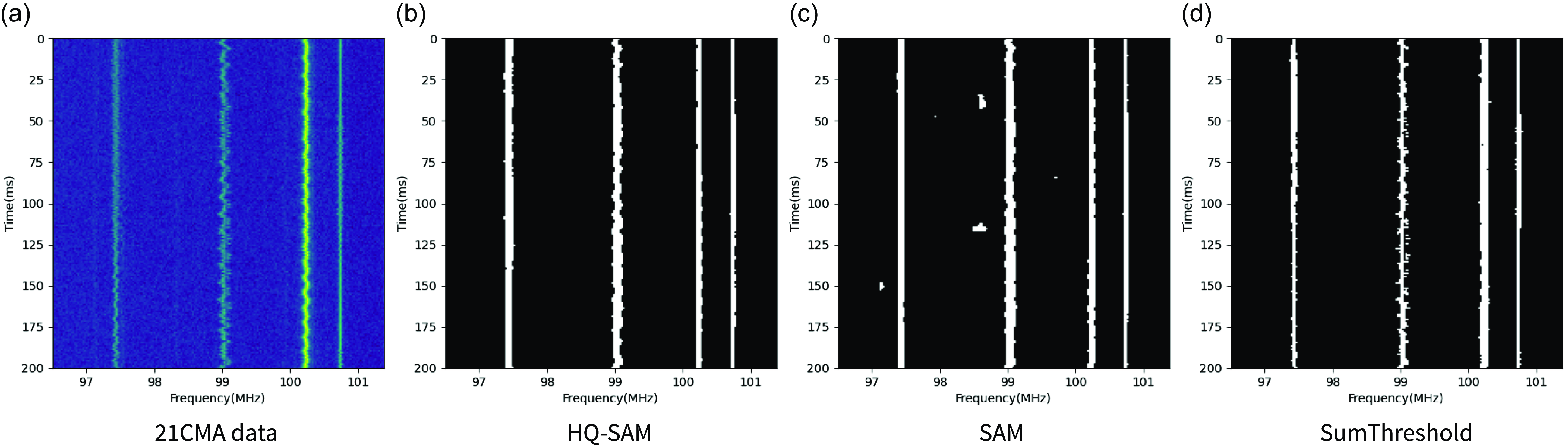
Figure 2. The raw data of the continuous narrowband RFI from the 21CMA and the detection results of three methods are shown in the following plots. The horizontal axis represents frequency, and the vertical axis represents time. (a) shows the raw data, which includes a large amount of continuous narrowband RFI. (b) shows the flagging results using HQ-SAM. (c) shows the flagging results using SAM. (d) shows the flagging results using the SumThreshold method. The white areas in the images correspond to the detected RFI.
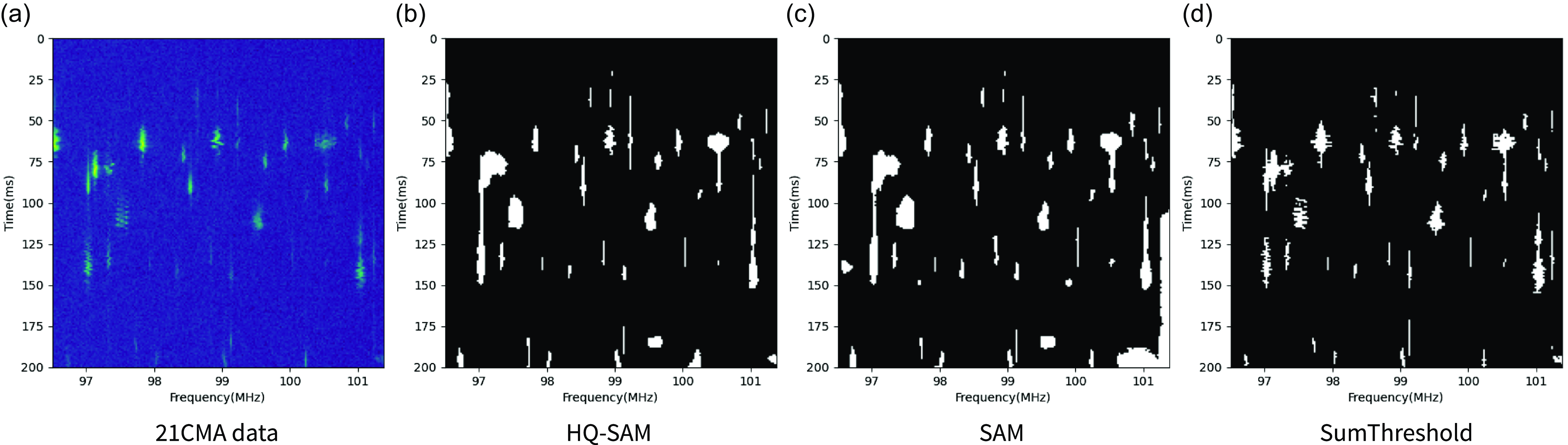
Figure 3. The same as in Fig. 2 but another example of the detection results of the 21CMA data.
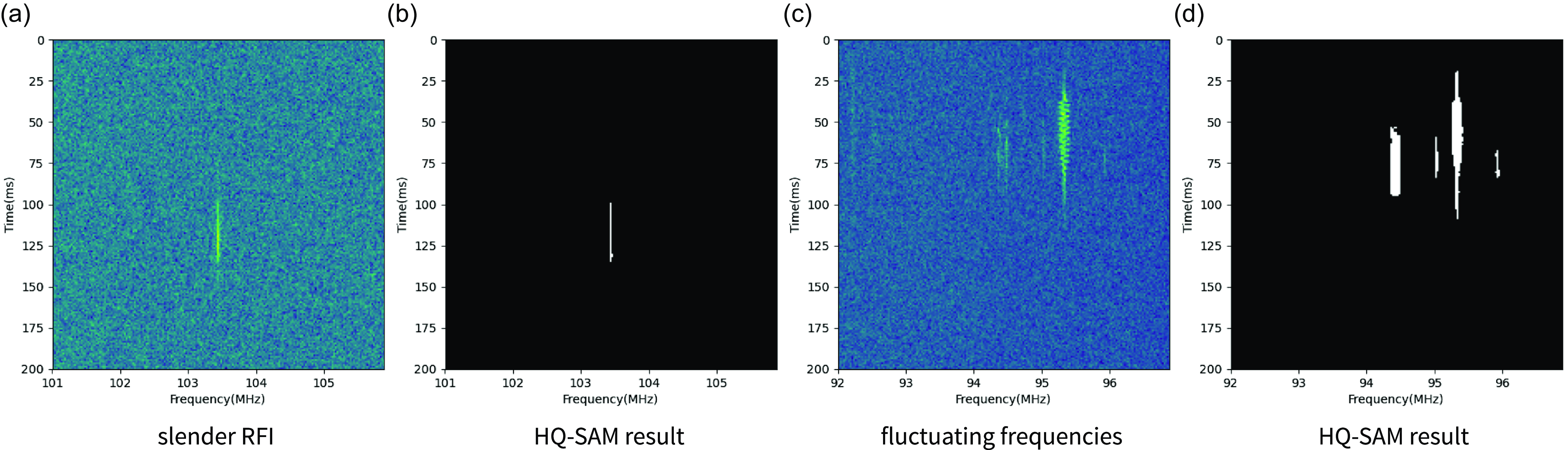
Figure 4. Classification of narrowband RFI in frequency. (a) is a common slender signal. (b) is the result of detecting (a) using HQ-SAM. (c) is RFI with fluctuating frequencies, and (d) is the detection result of (c) by HQ-SAM.
3.3 The results of HQ-SAM (SAM) of the 21CMA data
We conducted a preliminary search of the 21CMA observational data (4.6 TB) using HQ-SAM and identified that the majority of the RFI consists of narrowband RFIs. Additionally, there are instances of broadband RFI events that contaminate a large number of frequency channels (see Fig. 8). Based on the characteristics of RFI in time, frequency, and quantity, we divide narrowband RFI into three main categories, while broadband RFI is treated separately as a special case. As shown in Fig. 4, in addition to the common slender signals, narrowband RFIs demonstrate a frequency modulation pattern similar to FM radio signals. Fig. 5 shows that the duration of narrowband RFI can mainly be classified into two groups. Apart from the transient or short-duration signals with durations around 50–200 ms shown in Fig. 4, there are numerous continuous RFIs lasting for tens of seconds or more (the entire event of RFI is not fully displayed in Fig. 5). Furthermore, narrowband RFI is observed both sporadically as depicted in Figs. 4 and 5, and in large bursts dispersed across multiple frequency bands, as illustrated in Fig. 6. For continuous narrowband RFI, it is intriguing to find transitions between straight lines and polylines during transmission (Fig. 7). Fig. 8 illustrates the broadband signals detected by us, which span a frequency range of up to 20 MHz.
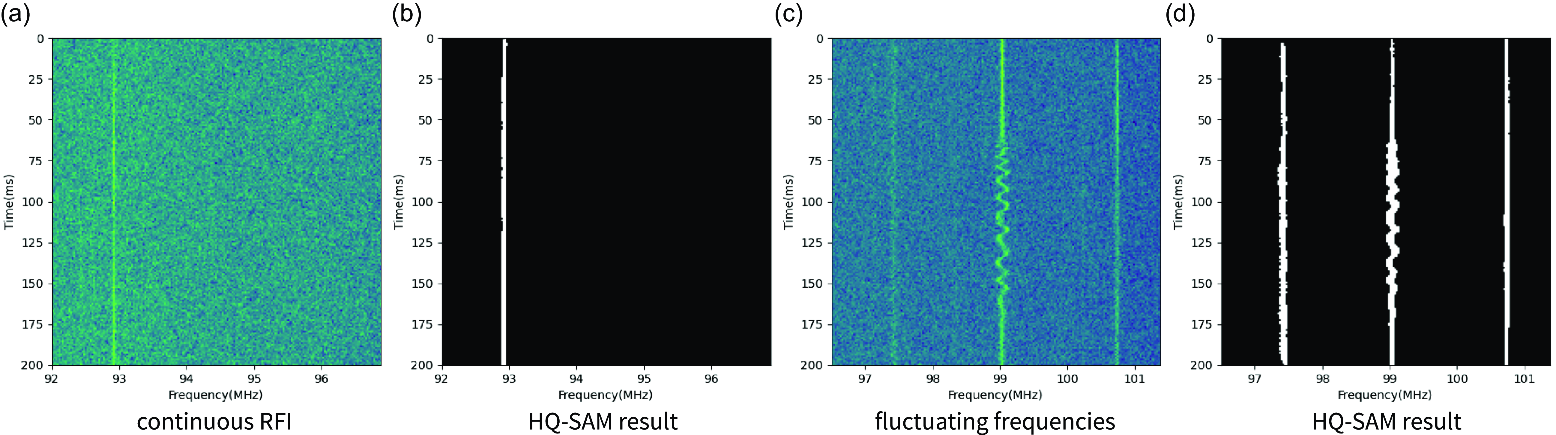
Figure 5. Two types of continuous RFI. (a) and (c) are respectively slender RFI and RFI with fluctuating frequencies similar to frequency modulation. Unlike the RFI in Fig. 4, which last only around 50–200 ms, these RFI last for tens of seconds or more (the entire event of RFI is not fully displayed here).
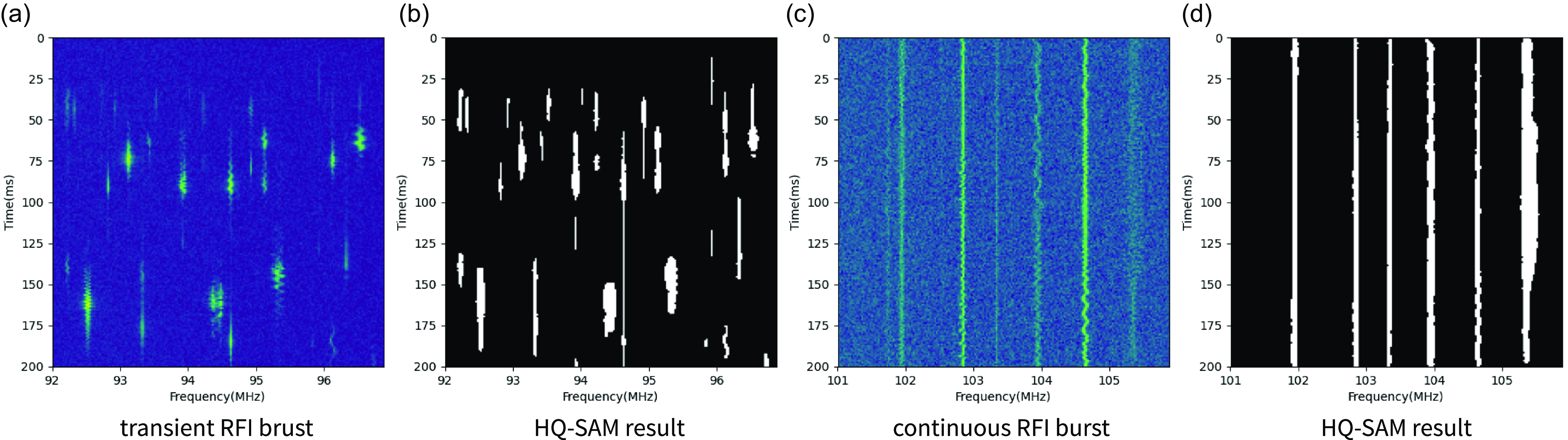
Figure 6. The bursts of transient RFI and continuous RFI.
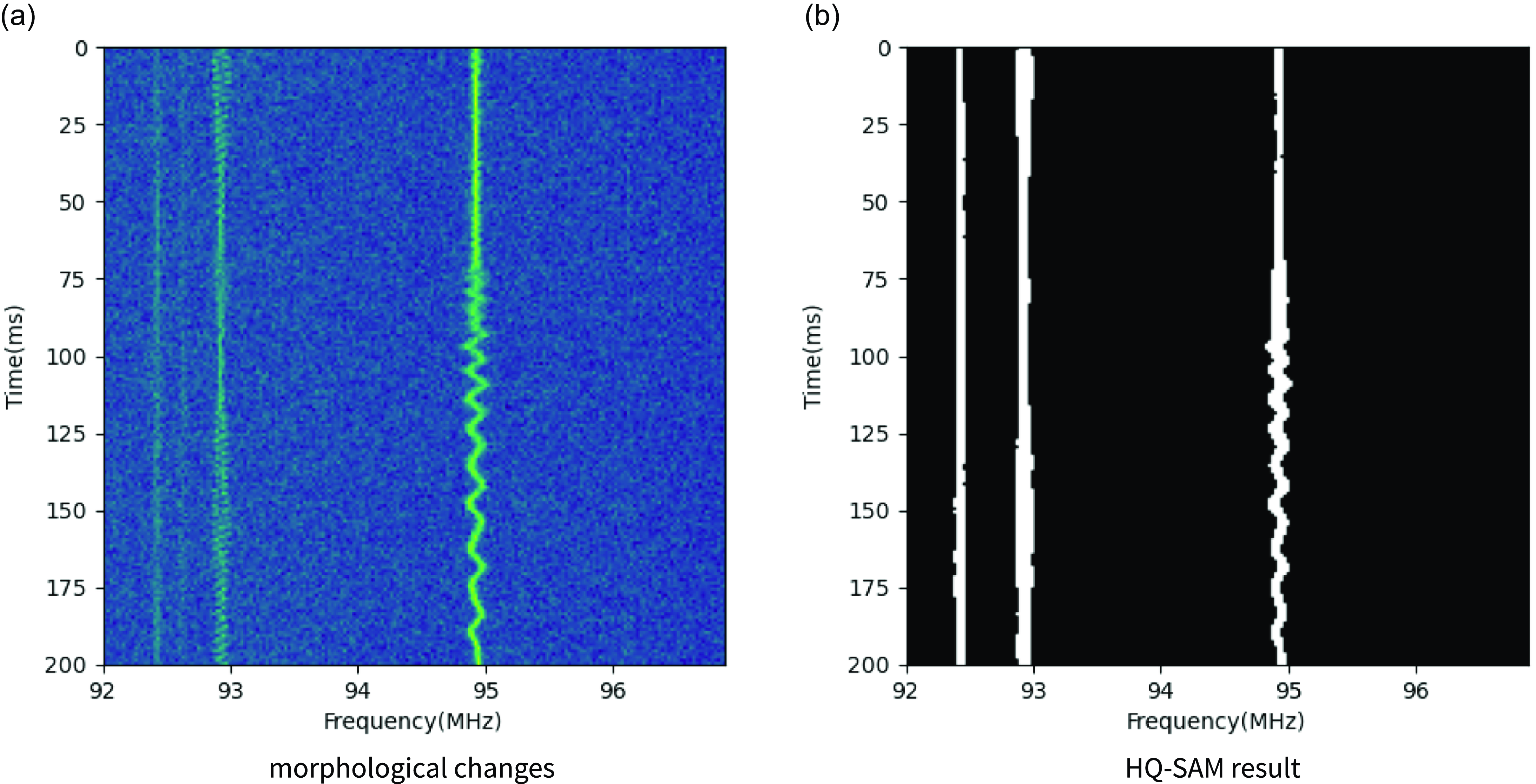
Figure 7. transitions between straight lines and polylines during transmission for continuous RFI.
According to Gao et al. (2022), we believe that the primary cause of transient narrowband RFI is the scattering of FM broadcasts by meteor trails. For the continuous narrowband signals, the number of events varies with time, similar to the variation in meteor events due to the Earth’s rotation. The quantity of narrowband RFIs far exceeds that of the known nearby FM broadcasts. In fact, there are no constant FM radio signals at the 21CMA site. Apart from the narrowband signals originating from FM broadcasts, the remaining sources require further investigation.
In summary, we find that HQ-SAM (SAM) performs comparably to the SumThreshold method when applied to real observational data from the 21CMA, especially in finding as many RFIs as possible. We conducted a sanity check of the detection results by comparing the results from HQ-SAM (SAM) with those from human visual inspection. HQ-SAM (SAM) effectively identifies most of the RFIs detected by human visual inspection. Furthermore, HQ-SAM outputs less noise and higher quality masks compared to SAM in actual detection results, thus confirming the assertion by Ke et al. (Reference Ke, Ye, Danelljan, Liu, Tai, Tang and Yu2023). In Appendix B, the results of the three methods for Figs. 2 and 3 are plotted pairwise on the same layer to show the differences in the masks obtained by each method.
However, HQ-SAM (SAM) also presents several issues worthy of optimisation: when two RFI events are too close in the waterfall plot, the model may classify them as a single RFI event; there is a certain amount of noise present in the output results; the segmentation of RFI profiles is relatively coarse; and although HQ-SAM (SAM) can identify some faint RFI, it still has limitations with extremely faint RFI signals, which are barely noticeable to the human eye as well. The SumThreshold method faces similar challenges.
4. RFI detection of simulation data
In this section, by mock RFI data, we can further evaluate the performance of the three methods and provide specific evaluation metrics to illustrate their respective strengths and weaknesses.

Figure 8. An example of broadband RFI which can contaminate frequency range of up to 20MHz.
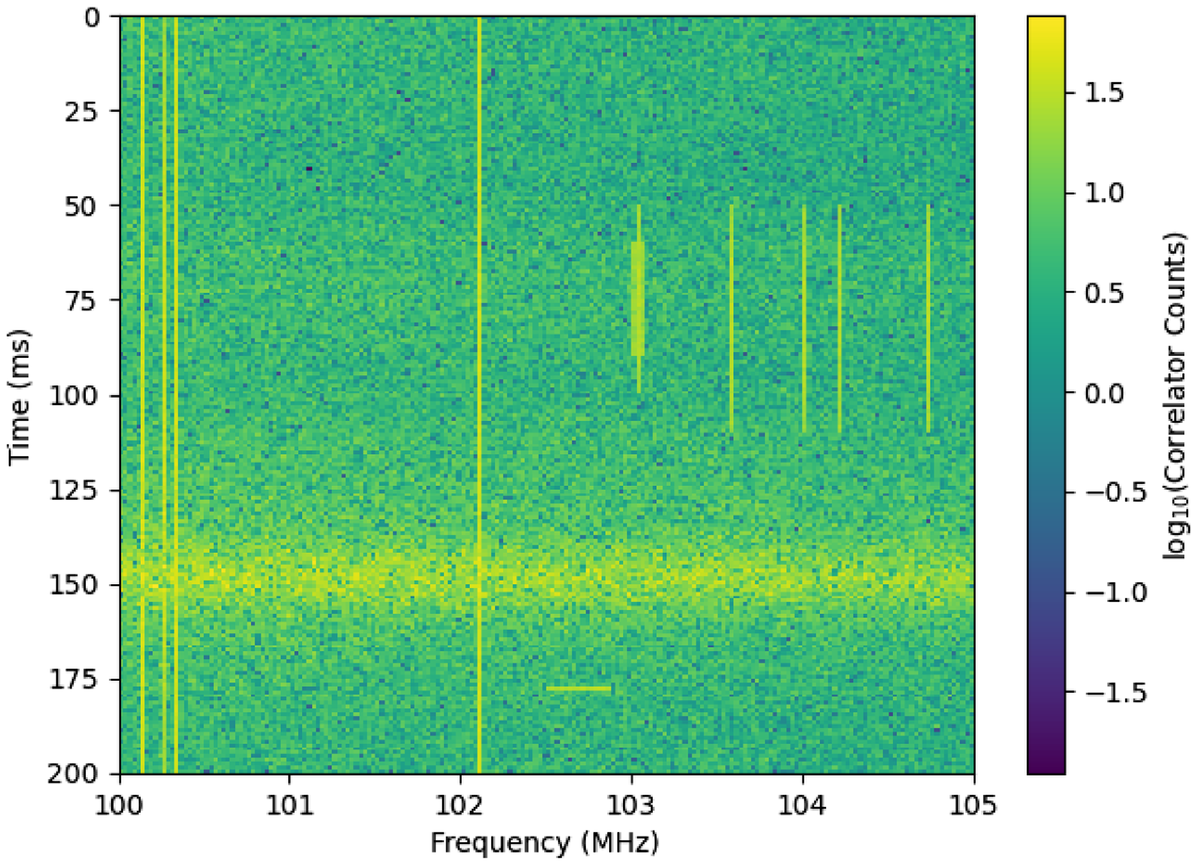
Figure 9. An example of Type A mock RFI, which contains dtv RFI and narrowband RFI.
4.1 RFI simulation
We use the hera_simFootnote
d
to simulate RFI signals. The hera_sim is a basic simulation package for HERA-like redundant interferometric arrays, which can also generate RFI (Chen & La Plante Reference Chen and La Plante2021; Kerrigan et al. Reference Kerrigan2019; Haomin et al. Reference Haomin, Deng, Wang, Mei, Xu, Smirnov, Deng and Wei2022; Liang et al. Reference Liang2023). There are two types of RFI data that have been created, each consisting of 300 waterfall plots with RFI signals, all of which are 200
 $\times$
200 in size. The horizontal axis of these waterfall plots represents frequency, and the vertical axis represents time. For the first type of mock RFI (as shown in Fig. 9), referred to as Type A, basic thermal noise and EoR-like visibilities are simulated using hera_sim. This tool allows us to generate several types of RFI, and we select narrowband RFI and RFI arising from digital TV channels (DTV RFI). The DTV RFI are set to be distributed with a probability of 0.005 over a certain frequency range and appear as rectangular blocks, with an amplitude approximately 0.71 mag higher than the background (in base-10 logarithm; the following is simplified to approximate numbers). Considering the characteristics mentioned in Section 3, including intensity variations, frequency fluctuations, and differences in durations (transient or continuous), we adjust the code for narrowband RFI to better reflect real-world scenarios. Hence, the following sorts of narrowband RFI can be observed in Fig. 9: continuous RFI with fixed intensity (0.84), continuous and transient RFI with intensity varying over time (0.54–0.84; 0.54–0.71), and a transient event with a noticeable frequency width (a simple imitation of RFI in Fig. 4c which has frequency fluctuations; 0.54–0.71). Within their respective frequency ranges, the probabilities of these events are 0.01, 0.01, and 0.04, respectively, and the transient event is set to appear with a probability of 0.6 per picture. It is worth mentioning that the SEEK package performs median normalisation on the data before applying the SumThreshold method. If there are continuous narrowband RFI that do not vary dramatically in intensity, they will be removed at this step, resulting in their undetection. We speculate that this may be because the designers did not anticipate facing this kind of RFI mitigation. In this paper, the code is modified to remove this normalisation step.
$\times$
200 in size. The horizontal axis of these waterfall plots represents frequency, and the vertical axis represents time. For the first type of mock RFI (as shown in Fig. 9), referred to as Type A, basic thermal noise and EoR-like visibilities are simulated using hera_sim. This tool allows us to generate several types of RFI, and we select narrowband RFI and RFI arising from digital TV channels (DTV RFI). The DTV RFI are set to be distributed with a probability of 0.005 over a certain frequency range and appear as rectangular blocks, with an amplitude approximately 0.71 mag higher than the background (in base-10 logarithm; the following is simplified to approximate numbers). Considering the characteristics mentioned in Section 3, including intensity variations, frequency fluctuations, and differences in durations (transient or continuous), we adjust the code for narrowband RFI to better reflect real-world scenarios. Hence, the following sorts of narrowband RFI can be observed in Fig. 9: continuous RFI with fixed intensity (0.84), continuous and transient RFI with intensity varying over time (0.54–0.84; 0.54–0.71), and a transient event with a noticeable frequency width (a simple imitation of RFI in Fig. 4c which has frequency fluctuations; 0.54–0.71). Within their respective frequency ranges, the probabilities of these events are 0.01, 0.01, and 0.04, respectively, and the transient event is set to appear with a probability of 0.6 per picture. It is worth mentioning that the SEEK package performs median normalisation on the data before applying the SumThreshold method. If there are continuous narrowband RFI that do not vary dramatically in intensity, they will be removed at this step, resulting in their undetection. We speculate that this may be because the designers did not anticipate facing this kind of RFI mitigation. In this paper, the code is modified to remove this normalisation step.
Inspired by the broadband streaks reported in Wilensky et al. (Reference Wilensky, Morales, Hazelton, Barry, Byrne and Roy2019) and the broadband event shown in Fig. 8, the second type of mock RFI, Type B, introduces a new category of broadband signals (0.24–0.54) with a probability of 0.6 per picture, while the other aspects remain the same as in the first type. Fig. 10 is an example of such simulated signals. There is a broadband event with intensity changing by frequency, set as a rectangle.

Figure 10. An example of Type B mock RFI. Compared to Type A, it includes an additional type of broadband RFI.
4.2 Evaluation metrics
By simulating, we obtain spectra data containing the RFI and the corresponding ground truth. Then, utilise HQ-SAM, SAM, and the SumThreshold method to recognise the mock signals and, respectively, compare the recognition results with the ground truth to get quantitative evaluation metrics.
The evaluation metrics used in this article include precision, recall, precision, and F1 score. They are defined as follows:
 \begin{equation} \textrm{Accuracy} = \frac{\textrm{TP+TN}}{\textrm{TP+TN+FP+FN}}\end{equation}
 \begin{equation} \textrm{Recall} = \frac{\textrm{TP}}{\textrm{TP+FN}}\end{equation}
 \begin{equation} \textrm{Precision} = \frac{\textrm{TP}}{\textrm{TP+FP}}\end{equation}
 \begin{equation} \textrm{F1} = \frac{2\times\textrm{Precision}\times\textrm{Recall}}{\textrm{Precision+Recall}}\end{equation}
In this work, the counts of true positive (TP), true negative (TN), false positive (FP), and false negative (FN) are based on individual pixels, where each pixel is classified as either RFI or non-RFI.
The evaluation results of the three methods for the Type A recognition task are shown in Table 1. And the evaluation results for Type B are shown in Table 2.
Table 1. Accuracy, Recall, Precision, and F1 Score of three methods for the Type A mock RFI recognition task.
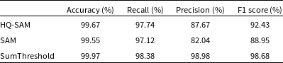
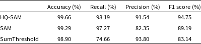
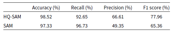
Table 2. Accuracy, Recall, Precision, and F1 Score of three methods for the Type B mock RFI recognition task.
4.3 Results
According to Section 4.2, we are able to provide quantitative evaluations for the three methods.
In RFI recognition tasks, RFI typically exhibit complex structures and characteristics. In the two types of simulated data, HQ-SAM outperforms SAM in terms of metrics (especially Precision), indicating that HQ-SAM demonstrates better performance than SAM, thus confirming the claims made in Ke et al. (Reference Ke, Ye, Danelljan, Liu, Tai, Tang and Yu2023).
For Type A mock data recognition, the SumThreshold method shows excellent performance with an F1 Score of 98.68%. HQ-SAM, without fine-tuning or structural additions, also performs commendably with an F1 Score of 92.43%. SAM, while capable of recognising most RFI, shows worse performance in Precision compared to the first two methods. This is because, under the same conditions, SAM outputs more miscellaneous items than HQ-SAM, which lowers the Precision score and, consequently, the F1 Score.
For Type B mock data recognition, where broadband RFI or large areas of RFI are present, HQ-SAM (and SAM) demonstrates superior performance compared to the SumThreshold method, with an F1 Score of 94.75% compared to 83.14%. Notably, HQ-SAM (and SAM) excels in Recall, achieving 98.19% versus 74.66% for the SumThreshold method. This high Recall is particularly crucial for our goal of identifying and removing as many RFI events as possible.
Since SAM outputs multiple masks and we use automatic evenly sprinkling points as prompts, there will be miscellaneous masks mixed with the masks we need. We use mask area and predicted Intersection over Union (IoU) limits to filter out these miscellaneous masks. Therefore, if one plans to use it, additional filtering conditions may be necessary from the start. In fact, manual inspection reveals that SAM and HQ-SAM actually achieve better performance metrics than those listed. This discrepancy arises because some miscellaneous and over-recognition masks, which overwrite the precise segmentation masks, were not filtered by our simple conditions, leading to a lower Precision score than what could actually be achieved.
In addition to the problems mentioned in Section 3.3, we note that for continuous narrowband RFI, which morphologically presents as a straight line and lasts the entire observation time, if it is too close to the edge of the image, the model may recognise the region between it and the boundary without properly identifying the narrowband itself. Similarly, when two narrowbands are too close together, both the RFI and the region between them may be identified as a single entity. As a result, the output masks in these cases are filtered out, which reduces the Recall score.
In summary, we conlcude that, on one hand, HQ-SAM can be used directly to identify RFI due to its strong generalisation capability and recognition ability. On the other hand, it is worth fine-tuning HQ-SAM (SAM) in this domain to optimise performance, or developing better automatic mask filtering methods to achieve more precise segmentation results.
4.4 Resource requirements and speed
Compared to the SumThreshold method, HQ-SAM (and SAM) does not require manual adjustment of thresholds and iteration counts. However, it does incur additional GPU requirements (the model can run on both CPU and GPU). Our server is equipped with a Tesla P100 PCIe 16 GB GPU. SAM using the vit_h checkpoint requires 6.5 GB of GPU memory, while HQ-SAM requires 10.5 GB.
Besides calculating evaluation metrics, we also measure the runtime of the three methods. HQ-SAM (and SAM) require more time compared to the SumThreshold method. Under the same conditions for HQ-SAM and SAM (
 $\textrm{points_per_side = 96}$
), SAM takes approximately four times longer than the SumThreshold method, while HQ-SAM takes nearly six times longer.
$\textrm{points_per_side = 96}$
), SAM takes approximately four times longer than the SumThreshold method, while HQ-SAM takes nearly six times longer.
For SAM, when
 $\textrm{points_per_side = 40}$
, the runtime is comparable to that of the SumThreshold method. For HQ-SAM, however,
$\textrm{points_per_side = 40}$
, the runtime is comparable to that of the SumThreshold method. For HQ-SAM, however,
 $\textrm{points_per_side = 34}$
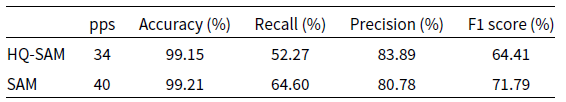
is required. In this case, for both Type A and Type B mock data recognition, Recall of the two models decrease significantly (for Type A, Recall of SAM and HQ-SAM decrease by 33% and 45%, respectively, while for Type B, the decreases are 20% and 30%), while Precision change little. Therefore, we do not recommend excessively reducing computational performance for the sake of speed. Regarding Type B, if we compare the performance of the three method using F1 Score, SAM and HQ-SAM achieve F1 Score that are roughly comparable to the SumThreshold method when
$\textrm{points_per_side = 34}$
is required. In this case, for both Type A and Type B mock data recognition, Recall of the two models decrease significantly (for Type A, Recall of SAM and HQ-SAM decrease by 33% and 45%, respectively, while for Type B, the decreases are 20% and 30%), while Precision change little. Therefore, we do not recommend excessively reducing computational performance for the sake of speed. Regarding Type B, if we compare the performance of the three method using F1 Score, SAM and HQ-SAM achieve F1 Score that are roughly comparable to the SumThreshold method when
 $\textrm{points_per_side = 64}$
and
$\textrm{points_per_side = 64}$
and
 $\textrm{points_per_side = 40}$
, respectively, with their runtime being approximately 2.2 times and 1.3 times that of the SumThreshold method. Specific details about the evaluation metrics can be found in 10.
$\textrm{points_per_side = 40}$
, respectively, with their runtime being approximately 2.2 times and 1.3 times that of the SumThreshold method. Specific details about the evaluation metrics can be found in 10.

Figure 11. Several types of SRB data used in the Detection. There are Type II-IV alone and in pairs. The horizontal axis represents time, while the vertical axis represents frequency.

Figure 12. Examples of successful detection for Type II-IV SRBs. The right side is the raw data, and the left side is the output masks.

Figure 13. Examples of detection failure for Type II-IV SRBs.
In some scenarios that require real-time processing, SAM may not be suitable due to the significant computational cost introduced by its image encoder. Many works have attempted to improve the efficiency of SAM. For example, MobileSAM (Zhang et al. Reference Zhang, Han, Qiao, Kim, Bae, Lee and Hong2023) distills the knowledge from the heavy image encoder to a lightweight one. To enhance the speed of SAM in recognising RFI, replacing the image encoder with a lightweight model may be a promising direction for our future efforts.
5. SRB detection by HQ-SAM
The intricate characteristics of SRBs pose significant challenges for their automatic detection and classification. Currently, there are few studies on deep learning for SRB detection, and they are often limited by insufficient training data. Many of these studies adopt methods such as transfer learning (Guo et al. Reference Guo, Wan, Hu, Wang and Yan2022) or SRB simulation (Scully et al. Reference Scully, Flynn, Gallagher, Carley and Daly2023) to address this problem. Here, we apply HQ-SAM in the detection of SRBs, aiming to determine whether it demonstrates strong zero-shot and generalisation capabilities in such applications.
5.1 SRB data
The SRB data for this study are images of SRBs observed by the Green Bank Solar Radio Burst Spectrometer (GBSRBS), provided by the National Radio Astronomy Observatory website.Footnote
e
The horizontal axis represents time, while the vertical axis represents frequency. According to the shape, frequency, and time length of the SRBs, these images are classified into three types: Type II, Type III, and Type IV (Guo et al. Reference Guo, Wan, Hu, Wang and Yan2022). We obtained a total of 636 images, all cropped to the size of 1225
 $\times$
645. Fig. 11 shows several types of SRB data: Type II-IV alone and in pairs.
$\times$
645. Fig. 11 shows several types of SRB data: Type II-IV alone and in pairs.
5.2 Detection results by HQ-SAM
Here, we present the detection results of HQ-SAM for SRB data in the form of output masks. Our goal is to recognise the presence of all SRB events in the data and accurately identify the main portions of these events. A small amount of over-marking or under-marking is acceptable. We overlay the masks onto the original images and manually check for differences. Detection is considered successful if the events are recognised and the corresponding masks align well with the SRB contours in the image. If events are undetected, detected incorrectly, or if the masks over-label or under-label by more than 30% area, even if the presence of the event has been detected, it is deemed a detection failure. Fig. 12 shows examples of successful detection for separate Type II-IV, while Fig. 13 demonstrates examples of failures for the corresponding types. A more comprehensive display of the detection results for all six types can be found in Appendix E. In the qualitative presentation of these results, the axes are omitted.
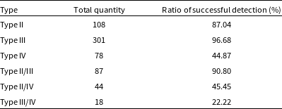
Table 3 shows the ratio of successful detections by HQ-SAM in recognising various SRBs, determined by manual inspection.
5.3 Results
When appearing isolated in spectrograms (e.g. Figs. 12 and 13), Type II and Type III SRBs can be effectively identified. However, HQ-SAM’s ability to recognise Type IV SRBs is weaker than for the first two types. Despite this, nearly half of the Type IV instances in this study are successfully detected.
In cases where two types of SRB events coexist (e.g. Figs. 17 and 18), effective detection is achieved when Type II and Type III occur simultaneously. However, when Type IV coexists with the other two types, recognising the Type IV is challenging. If there is overlap between Type IV and any of the other types, it further interferes with the detection of Type II and Type III because of Type IV morphological dispersion. During manual inspection, we notice that failures in detecting Type II/IV or Type III/IV data often occur due to difficulties in identifying Type IV SRBs, while Type II and Type III are frequently successfully identified.
Particularly, the large area, relatively diffuse distribution, and low intensity of Type IV SRBs – which often appear dim on spectrograms – make it challenging for the model to capture their features, affecting detection accuracy. Even when HQ-SAM successfully identifies Type IV SRBs, there may be errors in determining the exact contours of these events, leading to issues of over-labelling or under-labelling. For instance, Type IV SRBs and their surrounding background may sometimes be recognised as a single entity, resulting in masks that over-label with large areas. This issue is illustrated in Fig. E.3c and f, and such masks are often filtered out. The rare cases of detection failures of Type II, Type III, and Type II/III suggest that when these types of SRB or their backgrounds are too dim or diffuse, under-labelling can also occur.
In addition, the model’s inherent characteristics, instrument-generated stripes, and noise in the spectrogram can introduce various artefacts into the output masks, including small random points and large erroneous areas. Without appropriate filtering criteria, even if HQ-SAM accurately identifies the main structures of SRBs, the results may still be contaminated by these artefacts. Therefore, establishing effective filtering conditions for the masks is crucial.
Overall, HQ-SAM exhibits impressive performance in SRB detection tasks, particularly in identifying Type II and Type III SRBs. This is notable given that these results are achieved without additional model optimisation, and the model and its weights are readily accessible from the relevant website. Thus, we believe it is highly worthwhile to further explore the application of HQ-SAM in the field of SRB recognition.
6. Discussion
We have demonstrated that SAM and HQ-SAM hold significant potential for detecting various types of RFI and events. However, there is still room for improvement in the SAM and HQ-SAM models. For generalised models, specifying prompts helps filter the output masks, ensuring that the results focus on areas of interest. Since SAM cannot automatically generate suitable prompts for itself, we use the automatic segmentation mode provided by SAM, which involves evenly distributing points across the image. This method may lead to insufficient attention to important parts of the image. Alternatively, SAM offers the option to manually provide point or box prompts. Our experiments show that manually providing points results in more accurate target recognition compared to the automatic mode.
Nguyen et al. (Reference Nguyen, Phung and Cao2023) suggests using YOLO-v8 for initial image detection and obtaining bounding boxes around targets, which then serve as prompts to enhance segmentation quality. While this approach can improve precision in segmentation tasks, introducing a trained YOLO-v8 might reduce the model’s ability to detect unknown phenomena when aiming to identify all potential targets. A possible solution is to combine evenly distributed points with YOLO-v8, assigning different weights to each method based on specific needs. This combination could potentially improve recognition performance while preserving the model’s capacity to identify unknown events.
Additionally, implementing appropriate transfer learning for the model could be advantageous. Analysis of detection results from real and simulated RFI provided by HQ-SAM reveals that the model’s prior training, which primarily involved rich landscape images, inadequately addressed dim line images. This discrepancy sometimes leads the model to mistakenly interpret an RFI line as a boundary of an adjacent area. Therefore, targeted transfer learning can enhance the model’s ability to recognise and understand dim line features without introducing excessive data dependency or diminishing its capability to detect unknown phenomena.
It has been observed that the colour of an image significantly impacts the model’s recognition performance. The HQ-SAM model shows varying performance with different colour schemes. Specifically, for the simulated narrowband RFI discussed in Section 4, converting RGB images to pseudocolour greyscale produces coarser output masks, causing Precision to decline significantly (generally over 30%), as shown in Tables D.1 and D.2.
Table 3. The ratio of successful detection by HQ-SAM in recognising various SRBs.
These variations are likely due to the high-dimensional nature of RGB values, where even minor colour changes can produce significantly different feature vectors. This variability affects the model’s recognition accuracy. Therefore, it is crucial to consider factors such as image colour, detection target size, and image resolution when setting recognition targets to ensure optimal performance of the model.
7. Conclusions
In this paper, we apply HQ-SAM (SAM) to various scenarios of RFI and event detection in radio astronomy, demonstrating its impressive recognition and generalisation capabilities. For RFI detection, HQ-SAM (SAM) is utilised to identify both real RFI data from the 21CMA and simulated RFI data generated with the hera_sim package. The performance of HQ-SAM is compared with the SumThreshold method, showing superior results. Specifically, for broadband or large-area mock RFI, HQ-SAM achieves higher recall compared to the SumThreshold method, effectively reducing false negatives. Additionally, HQ-SAM demonstrates strong recognition abilities in detecting SRBs, including Type II and Type III bursts.
However, the model has some limitations, including the need for additional filtering due to miscellaneous items in the recognition results, coarse mask profiles, the computational limitations caused by the heavy image encoder, and the absence of semantic categorisation. Deep learning models often face challenges such as insufficient training data, data imbalance, over-reliance on training sets, and limited generalisation capabilities, as they are typically designed for specific tasks. Furthermore, designing and training models from scratch is a significant burden. HQ-SAM (SAM) stands out with its powerful generalisation capabilities, enabling easy deployment without extensive transfer learning or modifications. It functions as a plug-and-play solution and may help address or mitigate these common issues, making it a promising candidate for broader applications in astronomy.
Acknowledgements
We acknowledge the support of the Ministry of Science and Technology of China (grant No. 2020SKA0110200). YY acknowledges the support of the Key Program of National Natural Science Foundation of China (12433012).
Data availability statement
The data and code underlying this article can be shared on reasonable request to the corresponding author.
Competing interests
None.
Appendix A. Supplement to the SumThreshold Method
For two neighbouring samples, A and B, traditional thresholding involves independently comparing a statistic from each sample to a fixed threshold, which can lead to false positives and false negatives. In contrast, the VarThreshold method improves upon this by using combinatorial thresholding. It iteratively combines samples and compares them against a strictly decreasing series of thresholds,
 $\left \{ \chi _i \right \} ^N_{i=1}$
, where N is the number of iterations.
$\left \{ \chi _i \right \} ^N_{i=1}$
, where N is the number of iterations.
Initially, if A and B individually do not exceed the first threshold,
 $\chi_1$
, they are evaluated together with a lower threshold,
$\chi_1$
, they are evaluated together with a lower threshold,
 $\chi_2$
. If both samples exceed
$\chi_2$
. If both samples exceed
 $\chi_2$
, they are flagged. Otherwise, A, B, and the next neighbouring sample, C, are combined and compared with a further threshold,
$\chi_2$
, they are flagged. Otherwise, A, B, and the next neighbouring sample, C, are combined and compared with a further threshold,
 $\chi_3$
(Offringa et al. Reference Offringa, de Bruyn, Zaroubi and Biehl2010). This process continues iteratively and can be represented as:
$\chi_3$
(Offringa et al. Reference Offringa, de Bruyn, Zaroubi and Biehl2010). This process continues iteratively and can be represented as:
 \begin{equation}\begin{aligned} &flagv_M(v,t)=\exists i\in \left \{ 0...M-1 \right \} : \\ &\forall j\in \left \{0...M-1 \right \} :\left | R(v+(i-j)\Delta_v,t) \right | \gt \chi_{N(M)}\end{aligned}\end{equation}
where M is the number of samples. If the absolute values of all samples exceed the threshold
 $\chi_{N(M)}$
, these samples are flagged as RFI. Empirically,
$\chi_{N(M)}$
, these samples are flagged as RFI. Empirically,
 $M = \left \{ 1, 2, 4, 8, 16, 32, 64 \right \} $
has been found to be most effective and time-efficient, corresponding to 7 iterations.
$M = \left \{ 1, 2, 4, 8, 16, 32, 64 \right \} $
has been found to be most effective and time-efficient, corresponding to 7 iterations.
The strictly decreasing series of thresholds,
 $\left \{ \chi_i \right \}_{i=1}^N$
, is given by:
$\left \{ \chi_i \right \}_{i=1}^N$
, is given by:
 \begin{equation} \chi_i = \frac{\chi_1}{\rho^{\log_{2}{i} }}\end{equation}
Empirically,
 $\rho = 1.5$
is a suitable choice for both the VarThreshold and the subsequent SumThreshold methods.
$\rho = 1.5$
is a suitable choice for both the VarThreshold and the subsequent SumThreshold methods.
The SumThreshold method calculates the sum of statistics from M samples and compares it to M times the corresponding threshold,
 $\chi_{N(M)}$
. If samples flagged as RFI in previous iterations are encountered again, their values are replaced by the current iteration’s threshold. For example, consider the sample set
$\chi_{N(M)}$
. If samples flagged as RFI in previous iterations are encountered again, their values are replaced by the current iteration’s threshold. For example, consider the sample set
 $\left [ 2, 2, 5, 7, 2, 2 \right ]$
, where
$\left [ 2, 2, 5, 7, 2, 2 \right ]$
, where
 $\left [5,7\right ]$
are the RFI to be flagged. With thresholds
$\left [5,7\right ]$
are the RFI to be flagged. With thresholds
 $\left (6,4,3.16 \right )$
for 3 iterations, and sample numbers
$\left (6,4,3.16 \right )$
for 3 iterations, and sample numbers
 $\left (1,2,4 \right )$
, without applying the condition,
$\left (1,2,4 \right )$
, without applying the condition,
 $\left [ 2,2,5,7,2,2 \right ]$
would yield 4 false positives. By applying the condition,
$\left [ 2,2,5,7,2,2 \right ]$
would yield 4 false positives. By applying the condition,
 $\left [ 7 \right ]$
is flagged first, resulting in samples
$\left [ 7 \right ]$
is flagged first, resulting in samples
 $\left [ 2,2,5,4,2,2 \right ]$
. Then,
$\left [ 2,2,5,4,2,2 \right ]$
. Then,
 $\left [ 5,4 \right ]$
are flagged, and in the third iteration,
$\left [ 5,4 \right ]$
are flagged, and in the third iteration,
 $\left [ 2,2,3.16,3.16,2,2 \right ]$
yields no additional flags. Thus, only
$\left [ 2,2,3.16,3.16,2,2 \right ]$
yields no additional flags. Thus, only
 $\left [5,7 \right ]$
are flagged, avoiding false positives.
$\left [5,7 \right ]$
are flagged, avoiding false positives.
The SumThreshold method also allows for flagging sequences of samples with values below the thresholds. For a sample set
 $\left [ 1,3,4,7,4,3,1 \right ]$
, where
$\left [ 1,3,4,7,4,3,1 \right ]$
, where
 $\left [ 3,4,7,4,3 \right ]$
represent RFI with varying intensities, setting thresholds to
$\left [ 3,4,7,4,3 \right ]$
represent RFI with varying intensities, setting thresholds to
 $\left [ 6,4,3.16 \right ]$
and sample numbers to
$\left [ 6,4,3.16 \right ]$
and sample numbers to
 $\left [ 1,2,4 \right ]$
, the VarThreshold method flags only
$\left [ 1,2,4 \right ]$
, the VarThreshold method flags only
 $\left [ 7 \right ]$
, whereas the SumThreshold method flags
$\left [ 7 \right ]$
, whereas the SumThreshold method flags
 $\left [ 3,4,7,4,3 \right ]$
.
$\left [ 3,4,7,4,3 \right ]$
.
Appendix B. Supplement to RFI Detection Results of Real Data
We plot the detection results of the three methods for Figs. 2 and 3 pairwise on the same layer, using different colours to represent the differences in the masks obtained by each method. As shown in Figs. B.1a and B.2a, HQ-SAM demonstrates similar performance to the SumThreshold method when utilised on real observational data from the 21CMA, especially in finding as many RFIs as possible. Figs. B.1b, c, B.2b, and c show that SAM outputs more noise than HQ-SAM and the SumThreshold method.

Figure B.1. The differences in the masks obtained by each methods for Fig. 2 are as follows: (a) shows the difference between HQ-SAM and the SumThreshold method; (b) shows the difference between SAM and the SumThreshold method; and (c) shows the difference between HQ-SAM and SAM.

Appendix C. Supplement to RFI Recognition Speed
For SAM and HQ-SAM, their runtime are comparable to that of the SumThreshold method when
 $\textrm{points_per_side = 40}$
and
$\textrm{points_per_side = 40}$
and
 $\textrm{points_per_side = 34}$
. Under these parameter conditions, the evaluation metrics for Type A and Type B mock RFI recognition tasks can be found in Tables C.1 and C.2. Table C.2 also includes the evaluation metrics for SAM and HQ-SAM when they achieve F1 Score roughly comparable to the SumThreshold method at
$\textrm{points_per_side = 34}$
. Under these parameter conditions, the evaluation metrics for Type A and Type B mock RFI recognition tasks can be found in Tables C.1 and C.2. Table C.2 also includes the evaluation metrics for SAM and HQ-SAM when they achieve F1 Score roughly comparable to the SumThreshold method at
 $\textrm{points_per_side = 64}$
and
$\textrm{points_per_side = 64}$
and
 $\textrm{points_per_side = 40}$
, respectively.
$\textrm{points_per_side = 40}$
, respectively.
Table C.1. Accuracy, Recall, Precision, and F1 Score of SAM and HQ-SAM for the Type A mock RFI recognition task when the three methods have comparable runtime.
Note: pps refers to points_per_side.
Table C.2. Accuracy, Recall, Precision, and F1 Score of SAM and HQ-SAM for the Type B mock RFI recognition task when the three methods have comparable runtime or F1 Score.
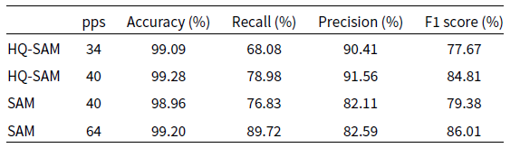
Note: pps refers to points_per_side.
Appendix D. Supplement to SAM’s Dependency of Colour
When the simulated narrowband RFI in Section 4 is converted from RGB format to pseudocolour greyscale images, the detection results of SAM and HQ-SAM are shown in Tables D.1 and D.2. By comparing the evaluation metrics in Tables 1 and 2, we observe that Recall remain largely unchanged, while Precision show a significant decline (generally over 30%). This is because when recognising pseudocolour greyscale images, the models tend to produce coarser boundaries for the detected narrowband RFI compared to images in colourmap ’viridis’ format, flagging more non-RFI signals in the surrounding areas.
Table D.1. Accuracy, Recall, Precision, and F1 Score of SAM and HQ-SAM for the Type A mock RFI recognition task when the images are in pseudocolour greyscale format.
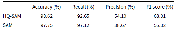
Table D.2. Accuracy, Recall, Precision, and F1 Score of SAM and HQ-SAM for the Type B mock RFI recognition task when the images are in pseudocolour greyscale format.
Appendix E. Supplement to Sular Radio Burst Detection Results
More examples of SRB detection results in Section 5.2 are presented here (as shown in Figs. E.1, E.2, and E.3).

Figure E.1. More examples of successful detection for separat Type II-IV SRBs are shown here.

Figure E.2. Examples of successful detection for pairs of Type II-IV SRBs.

Figure E.3. More examples of failed detection for different types of SRBs are shown here.


 Open access