Elasto-inertial rectification of oscillatory flow in an elastic tube

Abstract

The interaction between deformable surfaces and oscillatory driving is known to produce complex secondary time-averaged flows due to inertial and elastic nonlinearities. Here, we revisit the problem of oscillatory flow in a cylindrical tube with a deformable wall, and analyse it under a long-wave theory for small deformations, but for arbitrary Womersley numbers. We find that the oscillatory pressure does not vary linearly along the length of a deformable channel, but instead decays exponentially with spatial oscillations. We show that this decay occurs over an elasto-visco-inertial length scale that depends on the material properties of the fluid and the elastic walls, the geometry of the system, and the frequency of the oscillatory flow, but is independent of the amplitude of deformation. Inertial and geometric nonlinearities associated with the elastic deformation of the channel drive a time-averaged secondary flow. We quantify the flow using numerical solutions of the perturbation theory, and gain insight by developing analytic approximations. The theory identifies a complex non-monotonic dependence of the time-averaged flux on the elastic compliance and inertia, including a reversal of the flow. Finally, we show that our analytic theory is in excellent quantitative agreement with the three-dimensional direct numerical simulations of Pande et al. (Phys. Rev. Fluids, vol. 8, no. 12, 2023, 124102).

1. Introduction

The study of fluid flow in deformable geometries is important across various scientific domains, including physiology, biomedical engineering and lab-on-a-chip technologies (Gervais et al. 2006; Hardy et al. 2009; Das & Chakraborty 2010; Yeh et al. 2017). In laboratory settings, it is typical to fabricate fluidic systems with elastomeric materials (Ozsun, Yakhot & Ekinci 2013; Ushay, Jambon-Puillet & Brun 2023). The interplay between fluid flow and the mechanical response of soft material excites nonlinear flow phenomena that have received renewed interest in recent years (Holmes et al. 2013; Elbaz & Gat 2014, 2016; Christov et al. 2018; Christov 2022; Bureau, Coupier & Salez 2023; Rallabandi 2024). Many of these soft systems involve pulsatile, or more generally time-dependent flows (Kiran Raj, DasGupta & Chakraborty 2019; Dincau, Dressaire & Sauret 2020), where a common feature is the rectification of time-periodic driving into steady ‘streaming’ flows with non-zero time-average. This occurs due to a combination of inertial and geometric nonlinearities (Lafzi, Raffiee & Dabiri 2020; Bhosale, Parthasarathy & Gazzola 2022; Cui, Bhosale & Gazzola 2024). Inertial (advective) nonlinearities drive streaming even in rigid systems (Gaver & Grotberg 1986; Riley 2001; Zhang & Rallabandi 2023). Conversely, geometric nonlinearities due to oscillatory elastic deformation can elicit a secondary steady response even without inertia (Zhang et al. 2020; Kargar-Estahbanati & Rallabandi 2021; Bureau et al. 2023).

A configuration of particular interest involves time-periodic flows in compliant channels and conduits. Such flows occur naturally in physiological settings, e.g. in the flow of blood through both large arteries and small capillaries (Pedley 1980; Kiran Raj et al. 2019; Bäumler et al. 2020; Mirramezani & Shadden 2022), and the flow of air in the lungs. Oscillations may also occur spontaneously due to instabilities produced by large elastic deformations (Heil & Jensen 2003; Grotberg & Jensen 2004; Rust, Balmforth & Mandre 2008; Herrada et al. 2022). In engineered systems, interactions between oscillating flows and soft structures have found applications for flow control (Leslie et al. 2009), characterization of the dynamic properties of microchannel networks (Vedel, Olesen & Bruus 2010), and in the design and control of valveless pumps with flexible membranes (Biviano et al. 2022; Amselem, Clanet & Benzaquen 2023). Furthermore, driving oscillations at high frequencies allows inertial effects to be exploited in compliant systems to design switches (Collino et al. 2013) and pumps (Zhang et al. 2021).

The earliest quantitative model of oscillatory flows in compliant tubes was due to Womersley (1955) in the context of blood circulation. Womersley's work focused on the propagation of pressure pulses in long tubes and predicted a secondary flow due to deformation, but neglected the advective inertia of the fluid. Later work by Dragon & Grotberg (1991) accounted for both inertial and geometric sources of streaming in a semi-analytic treatment, again focusing on wave-like pulse solutions in long tubes. Recently, Pande, Wang & Christov (2023b) developed a reduced-order model of pulsatile flow in compliant conduits of finite length. Accounting for local fluid acceleration and elastic deformations, they obtained a nonlinear partial differential equation for the pressure distribution. The model yielded a secondary mean flow, which was found to be in agreement with three-dimensional (3-D) direct numerical simulations (DNS) in stiff tubes, but underpredicted the pressure in more compliant tubes, where elastic deformations were greater.

Here, we revisit this problem, but take a different approach and develop a systematic perturbation theory for small elastic deformations in the vein of Dragon & Grotberg (1991). The analysis reveals an amplitude-independent elasto-viscous parameter, which plays an important role, along with the Womersley number (a measure of fluid inertia), in controlling the structure of the flow. By developing an approximate analytic solution of the theory, we obtain insight into the geometric and inertial mechanisms that drive time-averaged streaming flow over a wide range of elasto-viscous parameters and Womersley numbers. We find that both effects are equally important in understanding the time-averaged streaming flow, and their combination fully captures the aforementioned DNS results.

The paper is organized as follows. Section 2 sets up the physical and mathematical problem, and identifies the important dimensionless groups that characterize the competition between viscous forces, fluid inertia and elastic deformation. In § 3, we develop a perturbation theory for small, but finite, deformations of the walls of the tube, and derive solutions for both the oscillatory and steady components of the flow. Analytic insight into the steady streaming is developed in § 4, which we compare with the results of Pande et al. (2023b) in § 5. Finally, § 6 concludes the paper by summarizing key findings and proposing future research directions.

2. Model set-up

We consider the flow of Newtonian fluid with dynamic viscosity $\mu$ and density $\rho$ in a cylindrical tube of length $L$ and equilibrium radius $R_0$ (figure 1). The walls of the tube have thickness $b$ and are made of an elastic material with Young's modulus $E$ and Poisson's ratio $\nu$. An oscillatory pressure with amplitude $P_i$ and angular frequency $\omega$ is applied at the inlet of the channel ($Z=0$) relative to the outlet of the channel ($Z=L$), which is maintained at zero pressure. This sets up a fluid flow $\boldsymbol {V}(\boldsymbol {X},T)$ and an associated pressure field $P(\boldsymbol {X},T)$ in the tube, where $T$ represents time. The stresses of the flow simultaneously deform the walls of the tube. We denote the instantaneous radial displacement of the tube by $U(Z, T)$, so that the instantaneous radius of the tube is $R_t(Z, T) = R_0 + U(Z,T)$.

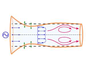
Figure 1. Schematic of set-up. A cylindrical tube with elastic walls is filled with a Newtonian fluid. Pressure oscillations applied at the inlet simultaneously drive fluid flow and deform the walls of the tube. The combination of boundary deformation and fluid inertia leads to a secondary flow with non-zero time average.

Of particular interest is the time-averaged flow in the tube, which occurs due to both the elastic deformation of the tube, and the advective inertia of the flow. As we will see, both effects are equally important in this system, and both are activated by elasticity.

2.1. Fluid flow

We assume that the fluid flow is incompressible, axisymmetric and devoid of swirl. The flow velocity is denoted by $\boldsymbol {V}(R, Z, T) = \{V_R(R, Z, T), V_Z(R, Z, T)\}$ in cylindrical coordinates, and satisfies the incompressible Navier–Stokes equations

(2.1a)\begin{gather} \rho\left(\frac{\partial\boldsymbol{V}}{\partial T}+\boldsymbol{V}\boldsymbol{\cdot} \boldsymbol{\nabla} \boldsymbol{V}\right)={-}\boldsymbol{\nabla} P+\mu\,\nabla^2\boldsymbol{V}, \end{gather}

(2.1b)\begin{gather}\boldsymbol{\nabla} \boldsymbol{\cdot} \boldsymbol{V}=0 . \end{gather}

It is useful to cast the continuity equation in terms of the flux $Q(Z, T) = 2 {\rm \pi}\int _0^{R_t} V_Z R \,\mathrm {d} R$ by writing $\partial _Z Q + \partial _T ({\rm \pi} R_t^2) = 0$, which leads to

(2.2) \begin{equation} \frac{\partial^{}Q}{\partial Z} + 2 {\rm \pi}(R_0 + U)\,\frac{\partial^{}U}{\partial T} = 0. \end{equation}

The flow is instantaneously no-slip at the walls of the deforming tube ($\boldsymbol {V}= \partial _{T}{R_t} \boldsymbol {e}_R$ at $R = R_t$) and satisfies symmetry conditions at the centreline ($\partial _{R}{V_Z} = 0$, $V_R = 0$ at $R = 0$). The pressure oscillates as $P_i \cos (\omega T)$ at the inlet ($Z = 0$) and is zero at the outlet ($Z = L$).

2.2. Elastic response of the tube

To close the problem, it is necessary to relate the deformation of the tube to the stresses in the flow. For thin-walled tubes ($b \ll R_0$), resistance to deformation occurs primarily due to elastic stresses generated by circumferential stretching of the tube (Landau & Lifshitz 1986; Audoly & Pomeau 2018). Focusing on slender channels $(R_0 \ll L)$, and anticipating the analysis of the subsequent sections, we approximate the normal stress exerted by the fluid on the tube by the fluid pressure $P(Z,T)$. For small radial deformations $U \ll R_0$ and negligible axial deformations, these arguments lead to the pressure-displacement relation

(2.3)\begin{equation} U(Z,T) = \frac{R_0^2 (1 - \nu^2)}{E b}\,P(Z,T). \end{equation}

This approximation has been shown (Anand & Christov 2020) to quantitatively capture 3-D DNS for the practically relevant case of nearly incompressible elastic solids ($\nu \approx 1/2$). More sophisticated membrane theories accounting for tension generated by viscous shear (Elbaz & Gat 2014, 2016; Rallabandi et al. 2021) have yielded results similar to (2.3) to leading order in the thickness of the tube walls. Models of the kind in (2.3), that relate local deformation to the local pressure (so-called Winkler foundation models), provide useful insight into flow–structure interactions in a wide range of systems (Dillard et al. 2018). The bending rigidity and inertia of the thin-walled tubes are small and have been neglected in this analysis; their magnitudes are estimated in Appendix A.

2.3. Non-dimensionalization

We rescale the equations by introducing dimensionless spatial coordinates (lowercase) $z=Z/ L$ and $r=R/ R_0$, and a dimensionless time $t=\omega T$. A balance between pressure gradients and viscous stresses sets a characteristic axial velocity scale $P_{i} R_{0}^{2}/(\mu L)$. By continuity, the radial velocity scale is $P_{i}R_{0}^{3}/(\mu L^{2})$. We define a dimensionless pressure $p$, and dimensionless velocity components $v_z$ and $v_r$, according to

(2.4a–c)\begin{equation} p =\frac{P}{P_i}, \quad v_z = \frac{V_z}{P_i R_0^2/(\mu L)}\quad \mbox{and} \quad v_r=\frac{V_r}{P_i R_0^3/(\mu L^2)}. \end{equation}

The problem is governed by four independent dimensionless parameters,

(2.5a–d)\begin{equation} \varepsilon = \frac{R_0}{L}, \quad \mathcal{W}=\frac{ \rho R_0^2 \omega}{\mu}, \quad\varLambda = \frac{P_i R_0 (1 - \nu^2)}{E b} \quad \mbox{and} \quad \sigma = \frac{\mu L^2 \omega (1 - \nu^2)}{E b R_0}. \end{equation}

Here, $\varepsilon$ is the aspect ratio of the tube, and is small by construction. The Womersley number $\mathcal {W}$ is the ratio of a viscous diffusion time scale $T_d = \rho R_0^2/\mu$ to the driving time scale $\omega ^{-1}$. The elasticity of the tube walls enters in two distinct ways. The parameter $\varLambda$ characterizes the amplitude of radial deformation relative to the radius of the tube, and scales with the inlet pressure amplitude $P_i$. The linear elastic framework (2.3) implicitly assumes that $\varLambda$ is small, and we use this condition explicitly in the analysis of later sections. In addition to the deformation amplitude, the flow–structure interaction introduces a time scale $T_{EV} = \mu L^2 (1 - \nu^2)/(E b R_0)$ over which elastic deformations relax against the viscous resistance of the fluid (see e.g. Elbaz & Gat 2014). The ratio of this relaxation time to the driving time defines the elasto-viscous parameter $\sigma$, which is analogous to the Deborah number in rheology. Similar quantities arise in other oscillatory fluid–elastic systems (Bickel 2007; Leroy & Charlaix 2011; Daddi-Moussa-Ider, Guckenberger & Gekle 2016; Zhang et al. 2022; Rallabandi 2024).

For typical parameters in arterial models and soft microfluidic systems, the aspect ratio $\varepsilon$ ranges from 0.001 to 0.1. The Womersley number $\mathcal {W}$ ranges from 1 to 100 at frequencies up to a few hundred Hz (Grotberg & Jensen 2004; Vishwanathan & Juarez 2020; Zhang & Rallabandi 2023), while the small deformation amplitude $\varLambda$ falls within the range 0.01 to 0.1 (Kiran Raj et al. 2019; Pande et al. 2023b). The elasto-viscous parameter $\sigma$ varies from 0.01 to 100, depending on the geometry of the tube ($\sigma$ is greater for longer tubes) and material properties; see Pande et al. (2023b). As we show in the following sections, the structure of the flow is governed primarily by $\mathcal {W}$ and $\sigma$, while $\varLambda$ sets the magnitude of the nonlinearity. We observe that $\mathcal {W}$ and $\sigma$ are similar in that they both represent the ratio of relaxation times to the driving time scale $\omega ^{-1}$. We will see later that $\mathcal {W}$ and $\sigma$ also control the spatial structure of the flow in similar ways.

3. Small-deformation theory for slender channels

We analyse the problem under a ‘long-wave’ theory for slender channels ($\varepsilon \ll 1$). The rescaled form of (2.1) in this limit is (Dragon & Grotberg 1991; Zhang & Rallabandi 2023)

(3.1a)\begin{gather} \mathcal{W} \left\{\frac{\partial v_z}{\partial t}+\frac{\varLambda}{\sigma}\, (\boldsymbol{v}\boldsymbol{\cdot} \boldsymbol{\nabla} ) v_z\right\}={-}\frac{\partial p}{\partial z}+\frac{1}{r}\,\frac{\partial}{\partial r}\left(r\, \frac{\partial v_z}{\partial r}\right) + O(\varepsilon^2), \end{gather}

(3.1b)\begin{gather}\frac{\partial p}{\partial r}=0 + O(\varepsilon^2), \end{gather}

(3.1c)\begin{gather}\boldsymbol{\nabla} \boldsymbol{\cdot} \boldsymbol{v} = \frac{1}{r}\,\frac{\partial^{}(r v_r)}{\partial{r}} + \frac{\partial^{}v_z}{\partial{z}} = 0, \end{gather}

where $\boldsymbol {v} \boldsymbol {\cdot } \boldsymbol {\nabla } = v_r\, \partial _r + v_z\,\partial _z$. Hereafter, we will not explicitly keep track of orders of $\varepsilon$. In dimensionless variables, the wall of the tube is instantaneously at $r = 1 + \varLambda \,p(z,t)$. Rescaling (2.2) yields

(3.2)\begin{equation} \frac{\partial^{}q}{\partial{z}} + 2 {\rm \pi}\sigma\,\frac{\partial^{}p}{\partial{t}}\,(1 + \varLambda p) = 0, \quad \text{where } q(z,t) = 2 {\rm \pi}\int_{0}^{1 + \varLambda p} v_z r \, {\rm d} r \end{equation}

is the instantaneous flux at any section of the channel, made dimensionless by $P_i R_0^4/(\mu L)$. The axial flow satisfies no-slip at the walls of the tube,

(3.3)\begin{equation} v_z = 0 \quad \text{at } r = 1 + \varLambda p, \end{equation}

and the pressure field $p(z, t)$ satisfies the boundary conditions

(3.4)\begin{equation} p|_{z= 0} = \cos t, \quad p|_{z= 1} = 0. \end{equation}

It is interesting to note that the elasto-viscous parameter $\sigma$ appears both in the continuity equation and in the advective term.

We develop a perturbation theory for small, but non-zero, deformation amplitude ${\varLambda \ll 1}$, and treat $\mathcal {W}$ and $\sigma$ as $O(1)$ parameters. We will see later that the theory also requires the mild restriction $\sigma \ll \varepsilon ^{-2}$ and $\mathcal {W} \ll \varLambda ^{-2}$, which are typically satisfied for the parameter ranges of interest. We seek a solution of the form

(3.5a)\begin{gather} p(z, t) = p_1(z, t) + \varLambda\,p_2(z, t) + O(\varLambda^2), \end{gather}

(3.5b)\begin{gather}\boldsymbol{v}(r, z, t) = \boldsymbol{v}_1(r, z, t) + \varLambda\,\boldsymbol{v}_2(r, z, t) + O(\varLambda^2), \end{gather}

where we have used (3.1b) to eliminate the dependence of pressure on the radial coordinate. The subscript 1 identifies the primary oscillatory flow, which scales linearly with the pressure amplitude $P_i$ but is independent of the amplitude of elastic deformation. Secondary flow quantities (subscript 2) are quadratic in the pressure amplitude and are associated with the finite amplitude of elastic deformation. Substituting the series expansion (3.5) into (3.1) and separating orders of $\varLambda$ yields the governing equations for the primary and secondary flow, which we discuss in the following subsections.

To expand the flux in powers of $\varLambda$, we first write $\int _0^{1 + \varLambda p} f(r) \, {\rm d} r = \int _0^{1} f(r) \, {\rm d} r + \int _1^{1 + \varLambda p} f(r) \, {\rm d} r$, for an arbitrary function $f(r)$. For small $\varLambda p$, the second integral can be approximated using the ‘rectangle rule’ as $\varLambda p\,f(1)$, up to errors of $O(\varLambda ^2)$. Applying this approximation to the integral in (3.2), and substituting (3.5), we obtain

(3.6a)\begin{gather} q(z,t) = q_1(z,t) + \varLambda\,q_2(z,t) + O(\varLambda^2), \quad \text{where} \end{gather}

(3.6b)\begin{gather}q_1 = 2{\rm \pi} \int_0^1 v_{1z} r \, {\rm d} r \quad \mbox{and} \quad q_2 = 2{\rm \pi} \left[\int_0^1 v_{2z} r \,{\rm d} r + \{(r v_{1z}) p_1\}|_{r =1}\right]. \end{gather}

A Taylor expansion of the no-slip condition (3.3) about $r = 1$ yields

(3.7)\begin{equation} v_{1z}+\varLambda \left(v_{2z}+ p_1\, \frac{\partial^{}v_{1z}}{\partial{r}}\right) + O(\varLambda^2) =0 \quad \text{at } r=1. \end{equation}

We now analyse the primary and secondary contributions to the flow.

3.1. Primary oscillatory flow

At $O(\varLambda ^0)$, advective inertia drops out of the momentum balance, yielding

(3.8)\begin{equation} \mathcal{W}\,\frac{\partial v_{1z}}{\partial t}={-}\frac{\partial p_1}{\partial z}+\frac{1}{r}\,\frac{\partial}{\partial r}\left(r\, \frac{\partial v_{1z}}{\partial r}\right), \quad \text{with } v_{1z}|_{r = 1} = \left.\frac{\partial^{}v_{1z}}{\partial{r}}\right|_{r = 0} = 0. \end{equation}

The continuity equation (3.2) at $O(\varLambda ^0)$ is

(3.9) \begin{equation} \frac{\partial^{}q_1}{\partial{z}} + 2 {\rm \pi} \sigma\,\frac{\partial^{}p_1}{\partial{t}} = 0. \end{equation}

Motivated by boundary conditions (3.4) for pressure, we seek solutions in terms of complex phasors oscillating as ${\rm e}^{{\rm i} t}$, whose real parts solve the physical problem. Writing the pressure as

(3.10)\begin{equation} p_1(z, t) = \text{Re}[\mathcal{P}_1 (z)\, {\rm e}^{{\rm i} t}], \end{equation}

the oscillating axial velocity is found to be

(3.11)\begin{equation} v_{1z}= \frac{1}{\alpha^2}\,\frac{\partial \mathcal{P}_1}{\partial z} \left(\frac{I_0(r \alpha )}{ I_0(\alpha ) }- 1\right) {\rm e}^{{\rm i} t},\quad \text{with }\alpha=\sqrt{{\rm i}\, \mathcal{W}}, \end{equation}

where $I_n(\cdot )$ is a modified Bessel function of the first kind of order $n$. It will be understood that only the real parts of complex oscillating quantities are physically meaningful. Equation (3.11) is the well-known velocity profile identified by Womersley (1955), which takes on a parabolic shape for small $\mathcal {W}$, and a plug-like profile with boundary layers of dimensional thickness $R_0 \mathcal {W}^{-1/2} = R_0 (\mu /(\rho \omega ))^{1/2}$ for large $\mathcal {W}$. From (3.6), the primary oscillatory flux is found to be

(3.12)\begin{equation} q_1=2{\rm \pi} \int^1_0 v_{1z} r \,\text{d}r={-}\frac{{\rm \pi}\,I_2(\alpha)}{\alpha^2\, I_0(\alpha)}\,\frac{\partial \mathcal{P}_1}{\partial z} \,\mathrm{e}^{\mathrm{i} t}. \end{equation}

Substituting (3.12) back into (3.9) leads to an equation governing the complex pressure:

(3.13)\begin{equation} \frac{\partial^2 \mathcal{P}_1}{\partial z^2}-k^2 \mathcal{P}_1=0,\quad \text{where } k=\sqrt{\mathrm{i}\sigma \, \frac{2\alpha^2\, I_0(\alpha) }{I_2(\alpha)}} \end{equation}

is a complex wavenumber. The above equation was also obtained by Ramachandra Rao (1983) in analysing linearized oscillatory flow in tapered elastic tubes, and a variant of it is given in Dragon & Grotberg (1991). The primary pressure oscillates as $p_1= \cos t = \text {Re}[ {\rm e}^{{\rm i}t}]$ at the inlet $z =0$, and decreases to zero at the outlet ($\kern0.7pt p_1=0$ at $z=1$), yielding the boundary conditions $\mathcal {P}_1(0) = 1$, $\mathcal {P}_1(1)=0$. With these conditions, (3.13) admits the solution

(3.14)\begin{equation} \mathcal{P}_1(z) = \frac{\sinh\{k(1-z)\}}{\sinh{k}}. \end{equation}

Thus we see that the primary pressure in a deformable tube decays as a spatially oscillating exponential. The limit $\sigma \to 0$ recovers the rigid case, where the pressure decreases linearly along the tube.

The complex wavenumber $k$ scales as $\sigma ^{1/2}$ and depends on $\mathcal {W}$ through $\alpha$. Figure 2(a) shows the variation of $k/\sqrt {\sigma }$ with $\mathcal {W}$, indicating both real and imaginary parts. In the viscous limit ($\mathcal {W} \ll 1$), $k$ approaches a constant $4 \sqrt {\mathrm {i} \sigma }$, indicating comparable rates of spatial decay and oscillation. For $\mathcal {W} \gg 1$, the real part of $k$ approaches $\sqrt {\sigma }$, while the imaginary part diverges as ${2 \sigma \mathcal {W}}$. Asymptotic behaviours for both small and large $\mathcal {W}$ are indicated in figure 2(a). Figure 2(b) shows both real and imaginary parts of $\mathcal {P}_1$ for different $\sigma$ at a fixed $\mathcal {W}$. For short elastic relaxation times ($T_{EV} \ll \omega ^{-1}$, or small $\sigma$) the elastic solid responds instantaneously to the inlet pressure, and the pressure drops linearly in the tube, similar to a rigid channel. For longer relaxation times ($T_{EV} \gtrsim \omega ^{-1}$, or $\sigma \gtrsim 1$), local deformation of the solid lags the inlet pressure, leading to a non-monotonic pressure distribution in the channel with comparable real (in-phase relative to the inlet) and imaginary (out-of-phase relative to the inlet) contributions (see figure 2(b) for $\sigma = 1$). At large $\sigma$ (and small $\mathcal {W}$), the pressure distribution decays axially from the inlet over a length scale $\ell _{EV} = L \sigma ^{-1/2} \propto (E b R_0 /(\mu \omega ))^{1/2}$, with spatial oscillations. We observe that this is analogous to how the Womersley velocity profile exhibits boundary layers of thickness $R_0 \mathcal {W}^{-1/2}$ for large $\mathcal {W}$. Thus $\sigma$ controls the axial structure of the flow similarly to how $\mathcal {W}$ controls its radial structure. At larger values, $\mathcal {W}$ influences both radial and axial flow features; see (3.13), (3.14) and figure 2. Figure 2(c) depicts profiles of $p_1(z,t)$ at different times over an oscillation cycle for the particular combination $\sigma = \mathcal {W} = 1$. The pressure distribution travels along the channel in a wave-like pattern, gradually diminishing further away from the inlet of the tube. It is interesting to note that the elasticity of the tube strongly controls the oscillatory flow through a competition between relaxation and driving time scales, even though the amplitude of deformation has not yet entered at this order in the analysis.

Figure 2. (a) Complex wavenumber $k$ as a function of $\mathcal {W}$, showing real and imaginary parts. Asymptotic expansions for large and small $\mathcal {W}$ are indicated by dashed curves. (b) Complex primary pressure $\mathcal {P}_1(z)$ at different $\sigma$ values, indicating real (solid) and imaginary (dashed) parts. The pressure decays linearly along the tube for small $\sigma$, whereas it decays exponentially for larger $\sigma$. (c) Pressure distribution at different times during an oscillation cycle for $\sigma =\mathcal {W}=1$, indicating wave-like behaviour.

3.2. Secondary steady flow

With insight into the oscillatory flow structure, we study the flow at $O(\varLambda )$, associated with finite deformation of the channel walls. We focus specifically on the rectified (time-averaged) part of this flow, which is associated with a net flux through the channel. We define the time average of a function over an oscillation cycle by $\langle\, f \rangle =(2 {\rm \pi})^{-1}\int _{\tau }^{\tau +2{\rm \pi} }f(t) \,\mathrm {d}t$. Averaging the momentum equation (3.1) and the no-slip condition (3.7), we find at $O(\varLambda )$ that

(3.15a)\begin{gather} \frac{\mathcal{W}}{\sigma} \langle \boldsymbol{v}_{1}\boldsymbol{\cdot} \boldsymbol{\nabla} v_{1z} \rangle={-}\frac{\partial \langle p_2 \rangle}{\partial z}+\frac{1}{r}\,\frac{\partial }{\partial r}\left(r\,\frac{\partial \langle v_{2z} \rangle}{\partial r}\right), \quad \text{with } \end{gather}

(3.15b)\begin{gather}\langle v_{2z} \rangle = v_{slip}(z) \stackrel{\text{def.}}{=} - \left.\left\langle p_1\, \frac{\partial^{}v_{1z}}{\partial{r}} \right\rangle\right|_{r =1} \quad \text{at } r = 1, \end{gather}

(3.15c)\begin{gather}\frac{\partial^{}}{\partial{r}} \langle v_{2z} \rangle = 0 \quad \text{at } r = 0. \end{gather}

Here, $v_{slip}(z)$ is an effective slip velocity satisfied by the secondary flow at the undeformed location of the tube walls, which arises as a consequence of the domain perturbation in (3.7). A useful rule for computing the time average of a product of oscillating complex quantities is $\langle \text {Re} [ A\, \mathrm {e}^{\mathrm {i} t}] \,\text {Re} [ B\, \mathrm {e}^{\mathrm {i} t}]\rangle = (1/2) \,\text {Re}[A^* B] = (1/2) \,\text {Re}[A B^*]$, where the asterisk denotes the complex conjugate (Longuet-Higgins 1998). We apply this rule to the definition (3.15b) to calculate the effective slip velocity

(3.16)\begin{equation} v_{slip}(z) = {\rm Re} \left[\frac{k\, I_1(\alpha)}{2\alpha\,I_0(\alpha)\,|{\sinh{k}}|^2} \cosh\{k (1-z)\}\sinh\{k^*(1-z)\}\right].\end{equation}

Note that only the real parts of secondary (time-averaged) flow quantities written with complex variables hold physical significance. This will be implied from this point onwards unless otherwise indicated.

The problem (3.15) is linear in $\langle v_{2z} \rangle$ and can be decomposed into three parts: (i) the velocity generated from the advective ‘body force’, which we denote $v_{2z}^{adv}$; (ii) the velocity associated with the geometric nonlinearity due to deformation, which manifests as the effective slip at $r =1$; and (iii) the velocity due to the secondary pressure gradient. Solving (3.15) shows that the time-averaged axial velocity has the general structure

(3.17)\begin{equation} \langle v_{2z} \rangle=\frac{1}{4}\,\frac{\partial \langle p_2 \rangle}{\partial z}\,(r^2-1) + v_{slip} + v_{2z}^{adv}, \end{equation}

where the advective contribution $v_{2z}^{adv}$ satisfies

(3.18)\begin{align} \frac{\mathcal{W}}{\sigma}\,\langle \boldsymbol{v}_{1}\boldsymbol{\cdot} \boldsymbol{\nabla} v_{1z} \rangle=\frac{1}{r}\,\frac{\partial }{\partial r}\left(r\,\frac{\partial v_{2z}^{adv}}{\partial r}\right), \quad \text{with } v_{2z}^{adv}|_{r = 1} = 0 \quad \mbox{and} \quad \left.\frac{\partial^{}v_{2z}^{adv}}{\partial{r}} \right|_{r = 0} = 0. \end{align}

The system (3.18) lacks a simple analytical solution due to the complicated radial dependence (involving products of Bessel functions) of the advective body force, so we solve it numerically using finite difference techniques to find $v_{2z}^{adv}$.

To obtain the secondary pressure, we first insert (3.17) into (3.6), which yields a general expression for the mean flux:

(3.19)\begin{equation} \langle q_2 \rangle = 2{\rm \pi} \left(-\frac{1}{16}\,\frac{\langle p_2 \rangle}{\partial z}+\frac{1}{2}\,v_{slip} + \int_{0}^{1}v_{2z}^{adv}(r, z)\,r \,\mathrm{d}r\right). \end{equation}

We then average the continuity equation (3.2) and collect terms at $O(\varLambda )$ to find that the time-averaged flux satisfies $\partial _{z} {\langle q_2 \rangle }+ 2 {\rm \pi}\sigma \langle \partial _{t}{p_2} + p_1\,\partial _{t}{p_1} \rangle = 0$. Observing that $\langle \partial _{t}{p_2} \rangle = 0$ and $\langle p_1\,\partial _{t}{p_1} \rangle = \langle \partial _{t}(p_1^2/2) \rangle = 0$, we find, unsurprisingly, that $\langle q_2 \rangle$ is a constant. We use this result to integrate (3.19) along $z$, noting that $\langle p_2 \rangle$ must vanish exactly at both ends of the tube, to obtain

(3.20)\begin{equation} \langle q_2 \rangle = 2 {\rm \pi}\int_0^1 \left(\frac{1}{2}\,v_{slip}(z) + \int_{0}^{1}v_{2z}^{adv}(r, z)\,r \,\mathrm{d}r\right) \mathrm{d} z. \end{equation}

Rearranging (3.19), the time-averaged pressure is therefore

(3.21)\begin{equation} \langle p_2 \rangle(z) = 16 \int_0^z \left(\frac{1}{2}\, v_{slip}(x) + \int_{0}^{1}v_{2z}^{adv}(r, x)\,r\, \mathrm{d}r\right)\,{{\rm d}\kern0.7pt x} - \frac{8 z}{\rm \pi}\,\langle q_2 \rangle. \end{equation}

Using (3.16) and the numerical solution to (3.18), we implement the integrals in (3.20) and (3.21) numerically to obtain $\langle p_2 \rangle (z)$.

The axial distribution of the secondary pressure is shown in figure 3 for different $\sigma$ and $\mathcal {W}$. Symbols represent the numerical solutions discussed above, and solid curves represent an analytic theory that we detail in § 4. As $\sigma$ approaches zero for a fixed $\mathcal {W}$ (representing a nearly rigid channel with a short elasto-viscous relaxation time), the secondary pressure distribution becomes parabolic. However, as $\sigma$ increases (slower elasto-viscous relaxation), the secondary pressure distribution becomes asymmetric, with the peak pressure rising and occurring closer to the channel inlet. This symmetry breaking arises because the primary flow – which is responsible for driving the secondary flow – now decays exponentially from the inlet over the length scale $L/k$ (figure 2b). Figure 3(b) shows the dependence on $\mathcal {W}$ at a fixed value of $\sigma = 1$ (moderately flexible channels). As $\mathcal {W}$ increases, the peak of the secondary pressure increases up to $\mathcal {W} \approx 5$. For larger $\mathcal {W}$, the pressure begins to drop, deviating from the established pattern. Thus the pressure distribution depends sensitively on both $\sigma$ and $\mathcal {W}$. Advective inertial effects become noticeable for $\mathcal {W}$ as small as $0.5$, and dominate for larger $\mathcal {W}$ (see figure 6 in Appendix B). These features highlight the interplay between channel elasticity, fluid inertia and viscous resistance to flow, emphasizing the importance of both $\sigma$ and $\mathcal {W}$.

Figure 3. Secondary flow pressure distribution for (a) fixed Womersley number $\mathcal {W}$ and (b) fixed elasto-viscous parameter $\sigma$. Symbols are results of numerical calculations, and curves represent the approximate analytic theory. Plot (a) shows the transition from parabolic distribution in quasi-rigid channels ($\sigma \to 0$) to asymmetric patterns in flexible channels ($\sigma$ increases). Plot (b) demonstrates increasing peak pressure with rising $\mathcal {W}$ in flexible channels for a range of $\mathcal {W}$, though the dependence becomes non-monotonic for $\mathcal {W} \gtrsim 5$.

As discussed previously, the flow varies axially over length scales set by $L$ and $L/k$, while radial gradients occur on scales $R_0$ and $R_0 \mathcal {W}^{-1/2}$ (where the latter quantity is the thickness of the oscillatory Stokes layer). The long-wave approximation used in the theory requires axial velocity gradients to be much smaller than radial ones, leading to the conditions $\varepsilon \ll 1$ and $\sigma \ll \varepsilon ^{-2}$. Furthermore, the theory requires small deformation amplitudes relevant to the relevant radial length scales of the flow, which yields the conditions $\varLambda \ll 1$ and $\mathcal {W} \ll \varLambda ^{-2}$. This condition on $\mathcal {W}$ also justifies neglecting the advective inertia of the secondary flow in (3.15) (Riley 2001).

4. Analytic approximation for the time-averaged flow

The complicated radial structure of the advective term in (3.18) precludes a simple analytic solution to $\langle p_2 \rangle$. We gain analytic insight by approximating the advective term, by first constructing approximate oscillatory velocity fields with simpler radial dependence (Appendix B). Our approximation to the primary axial velocity $\tilde {v}_{1z}$ shares the same centreline ($r = 0$) velocity as the exact solution (3.11), but replaces the radial dependence with a parabolic no-slip profile. Then we use the continuity equation to obtain an approximate primary radial velocity, $\tilde {v}_{1r}$; see (B1). We then construct an advective term $(\mathcal {W}/\sigma ) \langle \tilde {\boldsymbol {v}}_{1}\boldsymbol {\cdot } \boldsymbol {\nabla } \tilde {v}_{1z} \rangle$, which is given explicitly in (B2). This approximation is asymptotic to the exact result in the viscous regime $\mathcal {W} \ll 1$, where the oscillatory axial velocity profile is indeed parabolic. Additionally, (B2) preserves the centreline value and the $z$ dependence of the exact advective term for all $\mathcal {W}$, but presents a much simpler $r$ dependence that is now analytically tractable.

We use the result (B2) in place of the advective term in (3.18), and solve the resulting equation to obtain an explicit analytic approximation to $v_{2z}^{adv}$; see (B3). Substituting this result into (3.20), we find that the mean flux is

(4.1a)\begin{gather} \langle q_2 \rangle(\mathcal{W}, \sigma) = \frac{\lambda {\rm \pi}}{8} \left[ \left(\frac{\cosh \{2 k_r\} - 1}{k_r}\right) + \mathrm{i} \left(\frac{ \cos \{2 k_i\} - 1}{k_i}\right)\right], \quad \text{where} \end{gather}

(4.1b)\begin{gather}\lambda (\mathcal{W}, \sigma)\approx \underbrace{\frac{ k\,I_1 (\alpha)}{|{\sinh{k}}|^2\,\alpha\,I_0(\alpha) }}_{{effective\ slip}} + \underbrace{\frac{3 k^*}{32 \sigma} \left| \frac{k}{\sinh{k}}\,\frac{I_0(\alpha)-1}{\alpha\, I_0(\alpha)}\right|^{2}}_{advective\ inertia}, \end{gather}

with $k_r = \text{Re}[k]$ and $k_i = \text{Im}[k]$. The complex quantity $\lambda (\mathcal {W}, \sigma )$ (the real part is not implied in (4.1b)) is a scale factor comprising a contribution from the effective slip $v_{slip}$ (which arises directly from the change in geometry due to deformation) and another from the advective inertia of the primary flow. We recall that $\alpha$ and $k$ depend on $\mathcal {W}$ and $\sigma$; see § 3.1. Using (3.21), the approximate secondary pressure is

(4.2)\begin{align} \langle p_2 \rangle(z; \mathcal{W}, \sigma) &= \lambda(\mathcal{W}, \sigma) \left[ \left(\frac{z + (1-z)\cosh\{2k_r\}-\cosh\{2k_r (1-z)\}}{k_r}\right)\right. \nonumber\\ &\quad + \left.\mathrm{i}\left(\frac{z + (1-z)\cos\{2k_i\}-\cos\{2k_i (1-z)\}}{k_i}\right)\right]. \end{align}

We note that the only source of approximation is in the advective term of $\lambda$; (4.1) and (4.2) are otherwise faithful reproductions of the exact solution to (3.15).

Figure 3 shows the theoretical pressure (4.2) (solid curves) alongside ‘exact’ (numerical) solutions (symbols). The theory is in excellent quantitative agreement with numerical calculations, up to $\mathcal {W}$ close to 10; for instance, with $\sigma =1$, the error in the pressure is approximately $5\,\%$ at $\mathcal {W} =10$.

As expressed in (4.1), a non-zero time-averaged flux occurs due to the combined effect of geometric nonlinearities (quantified by the effective slip) and the inertial body force. The geometric mechanism is a generic feature of an oscillating flow in a conduit with an oscillating area of cross-section (Zhang et al. 2021; Pande, Boyko & Christov 2023a), while inertial pumping occurs due to Reynolds stresses generated at the walls of the tube. The secondary flux is generally positive, associated with net pumping of fluid towards $z = L$, but varies for different values of $\sigma$ and $\mathcal {W}$, as shown in figure 4. The flux becomes independent of both $\mathcal {W}$ and $\sigma$ at small $\mathcal {W}$, converging to the value ${\rm \pi} /8$. When $\sigma$ is small (a relatively rigid channel), the flux decreases as $\mathcal {W}$ increases. It is striking that the flux eventually becomes negative – fluid is pumped towards the source of pressure oscillations – at sufficiently large $\mathcal {W}$ for small $\sigma$. However, for more flexible channels (larger $\sigma$), the secondary flux generally increases with $\mathcal {W}$, albeit non-monotonically. The flux saturates at larger values of $\mathcal {W}$, and stays below unity. The dependence on $\sigma$ at fixed $\mathcal {W}$ is similarly complicated, displaying a non-monotonic behaviour until saturating at large $\sigma$. The theory (4.1) (solid curves in figure 4) is in excellent agreement with numerical results (symbols) across all parameter values, and reproduces the generation of negative fluxes at small $\sigma$ and large $\mathcal {W}$, as well as the non-monotonic dependence on $\sigma$ and $\mathcal {W}$. The appearance of $k_i$ in the argument of a cosine in (4.1) suggests that this non-monotonicity is due to the spatial oscillations of the primary pressure.

Figure 4. (a) Secondary flux for different $\sigma$ and $\mathcal {W}$. In the case of small $\sigma$, the flux decreases as $\mathcal {W}$ increases, reaching negative values at large $\mathcal {W}$. As $\sigma$ increases, there is a general trend of increased secondary flux, which saturates at approximately 1 for large $\mathcal {W}$. (b) Example secondary flow visualization for $\sigma =0.01$ and $\mathcal {W}$. In a quasi-rigid channel, small $\mathcal {W}=1$ (top) induces a secondary flow from inlet (the source of the oscillatory pressure) to outlet (held at zero pressure), while larger $\mathcal {W}$ leads to net flow from outlet to inlet. Colour bars indicate dimensionless flow speed.

We first analyse the limit $\sigma \ll 1$, where the elasto-viscous relaxation time is much smaller than the period of oscillation. The walls of the tube respond quasi-statically to the oscillating flow, and the pressure decays linearly along the tube. In this limit, (4.1) becomes

(4.3)\begin{equation} \langle q_2 \rangle \sim \frac{\rm \pi}{8} \left(\frac{2\,I_1(\alpha)}{\alpha\,I_0(\alpha) } - \frac{3\,I_0(\alpha)}{8\,I_2(\alpha)} \left|\frac{I_0(\alpha)-1}{I_0(\alpha)}\right|^2\right) \quad \text{as } \sigma \to 0. \end{equation}

The first term is due to the slip velocity, while the second term is the contribution of inertia. It is interesting to note that advective inertia survives even in the quasi-rigid limit $\sigma \to 0$ (even as $\boldsymbol {v} \boldsymbol {\cdot } \boldsymbol {\nabla } \boldsymbol {v}$ becomes vanishingly small) due to the appearance of $\sigma ^{-1}$ in front of the advective term in (3.15). Plotting each term separately shows that the contribution of slip is always positive, whereas the contribution of inertia is always negative for $\sigma \to 0$. The inertial term is small for small $\mathcal {W}$, leading to a positive, slip-dominated mean flow. At larger $\mathcal {W}$, the contribution of inertia to the flux outweighs that of the slip, leading to a negative mean flow. From (4.3), we find that the transition from positive to negative flux occurs at $\mathcal {W} \approx 6.9$, consistent with the $\sigma = 0.01$ curve in figure 4. Streamlines of the steady flow across this transition are plotted in figure 4, showing that the flow near the wall $r = 1$ (due to the effective slip) is always to the right even as the net flow changes sign with $\mathcal {W}$. A similar analysis of (4.2) shows that the secondary pressure has the form

(4.4)\begin{equation} \langle p_2 \rangle \sim \frac{8 \langle q_2 \rangle}{\rm \pi}\, z (1-z) \quad \text{for } \sigma \to 0. \end{equation}

The reversal in flux is thus accompanied by a reversal in the pressure. For small $\mathcal {W}$ (in addition to small $\sigma$), we find

(4.5)\begin{equation} \langle q_2 \rangle \sim \frac{\rm \pi}{8} \left( 1 - \frac{5 \mathcal{W}^{2}}{96} + O(\mathcal{W}^3) \right) \quad \text{for } \sigma \to 0. \end{equation}

The leading term is consistent with past work (see (38) of Pande et al. 2023b), while the second term differs due to the inclusion of advective inertia here.

These behaviours change sensitively as $\sigma$ increases even slightly from zero. Both the slip and advective contributions become more positive with growing $\sigma$. At $\sigma \approx 0.1$, the reversal of flux with $\mathcal {W}$ no longer occurs (figure 4a). For $\sigma \gtrsim 0.2$, the advective term becomes positive at all $\mathcal {W}$, thus aiding the slip velocity. As a result, the flux grows with $\mathcal {W}$ when $\sigma \gtrsim 0.2$, in contrast to the $\sigma \ll 1$ case (figure 4). The flux eventually saturates for large $\sigma$, once again becoming independent of it. In the limit, and for small $\mathcal {W}$, (4.1) yields

(4.6)\begin{equation} \langle q_2 \rangle \sim \frac{\rm \pi}{8} \left( 1 + \frac{5 \mathcal{W}}{16} + O(\mathcal{W}^2)\right) \quad \text{as }{\sigma \to \infty}. \end{equation}

We observe that the flux increases linearly with $\mathcal {W}$ at large $\sigma$, in contrast to the quadratic decrease at small $\sigma$ in (4.5). The contribution of inertia to the secondary flux becomes noticeable for $\mathcal {W} \gtrsim 0.5$, and may dominate for larger $\mathcal {W}$; see figure 6.

5. Comparison with the simulations of Pande et al. (2023b)

Pande et al. (2023b) conducted 3-D DNS of the problem, utilizing the svFSI finite-element solver of the open-source cardiovascular modelling software SimVascular (Updegrove et al. 2017; Lan et al. 2018). These simulations model the solid as a Kirchhoff–Saint Venant hyperelastic material, and fully resolve the two-way coupled time-dependent fluid–structure interaction (Zhu et al. 2022).

Figure 5(a) shows the pressure distribution $p(z,t)$ at different times over an oscillation cycle, comparing DNS (square symbols) and our analytic theory (curves), which use the approximation $p(z,t) \approx p_1(z,t) + \varLambda \langle p_2 \rangle$. We note that in the theory, we do not resolve the time-dependent part of $p_2$, though the error from this omission to the instantaneous pressure (which is dominated by $p_1$) is small. The agreement is excellent for $\sigma =0.6$ and $\mathcal {W}=1$, with no adjustable parameters. There is no discernible difference between our approximate analytical solutions and our numerical solutions for these parameters.

Figure 5. Comparison between the present analytic theory (curves) with the 3-D DNS of Pande et al. (2023b) (symbols), with $\varepsilon = 0.0667$ and $\varLambda = 0.05$. (a) Instantaneous pressure distribution over an oscillation cycle for $\sigma =0.6$ and $\mathcal {W}=1$. (b) Time-averaged pressure for different $\sigma$ and $\mathcal {W}$.

Figure 5(b) shows the time-averaged part of the pressure $\langle p \rangle /\varLambda = \langle p_2 \rangle$, comparing again the DNS (symbols) and our theoretical result (4.2) (curves). For different combinations of $\mathcal {W}$ and $\sigma$, the analytic theory captures the DNS remarkably well, again with no adjustable parameters. The deviations near $z = 0$ are likely due to the boundary conditions in the DNS being enforced only approximately. Our numerical calculations and analytic theory (cf. § 3.2) are identical to within the thickness of the curves in figure 5.

In addition to performing DNS, Pande et al. (2023b) developed a reduced-order model that accounted for the local acceleration of the fluid but neglected its advective inertia. That model, when solved numerically, recovered the DNS results for $\mathcal {W} \lesssim 1$ with $\sigma = 0.06$, but deviated for larger $\mathcal {W}$ and $\sigma$ ($\varLambda$, $\mathcal {W}$ and $\sigma$ here are equivalent to the quantities $\beta$, $\alpha ^2$ and $2 {\rm \pi}\, \text {St}_f\,\beta$, respectively, in Pande et al. 2023b). The agreement of our theory with the DNS shows that these deviations can be almost entirely understood by accounting for the advective inertia of the oscillatory flow. While additional geometric or material nonlinearities associated with the response of the elastic solid may indeed be important for larger deformations, they do not appear to play a significant role for $\varLambda = 0.05$. It remains to be seen how far the present theory can be pushed before departures from DNS become appreciable.

6. Conclusions

We have shown how the combination of fluid inertia and elastic deformations rectifies oscillatory driving in compliant channels into steady secondary flows. We have quantified these features by developing a long-wave perturbation theory for slender channels and small elastic deformations. The amplitude of deformation governs the magnitude of nonlinearities driving steady flow. The structure of the flow, however, is independent of this amplitude, and depends instead on two frequency-dependent parameters: the Womersley number $\rho R_0^2 \omega /\mu$, which measures a momentum diffusion time scale against the time scale of driving, and an elasto-viscous parameter $\mu \omega L^2 (1 - \nu ^2)/(E b R_0)$, which is the ratio of an elasto-viscous relaxation time to the driving time scale. The precise combination of these parameters controls the spatial structure of the oscillatory flow, which in turn determines the relative importance of geometric nonlinearities (due to deformation) and advective nonlinearities (due to fluid inertia) in driving time-averaged flow. Using judicious approximations for the advective inertia, we obtained closed-form analytic approximations that quantitatively recover 3-D DNS across the entire parameter space.

The insights derived from the present work enable systematic understanding and efficient quantification of time-dependent fluid–structure interactions in practically relevant settings. Future work may account for the effect of a finite bending rigidity and the inertia of the elastic material. It would be equally interesting to quantify the effects of internal dissipation in the solid, which would be relevant in practical systems, particularly at large frequencies (see e.g. Anand & Christov 2020). We expect that the small-deformation framework developed here could be expanded to accommodate these features in order to gain substantial efficiencies over DNS. The ideas developed here thus hold the potential to influence advancements in engineered and naturally occurring systems such as cardiovascular physiology, biomedical engineering and microfluidic device design.