1. Introduction
Research on quantitative trait loci (QTLs) often provides information on multiple complex traits that have well-established causal relationships. For example, in wheat genetics, it is common to collect data on grain yield (GRYL) and yield components such as thousand kernel weight (TKW), spikes per square metre (SPSM) and kernels per spike (KPS), where the causal relationships among these traits are well-established (Fig. 1), because yield components develop sequentially with later-developing components under the control of earlier-developing ones (Dofing & Knight, Reference Dofing and Knight1992). The primary goal of QTL mapping is to locate regions or genes that are associated with quantitative traits. The commonly used procedures capture only total QTL effects while providing no understanding of direct and indirect effects. However, these direct and indirect effects can help answer important questions that are not addressed by examining the total effect alone. For instance, a pleiotropic QTL can have a positive direct effect on GRYL, but a negative effect on a yield component. Without knowing the full pathway of the causal relationship, a breeder might select against the yield component QTL thinking it only affects the yield component detrimentally, not knowing that it is actually beneficial to the important trait of GRYL. Thus, the total effect can provide a misleading impression. To understand the genetic effects of a QTL thoroughly, it is necessary to understand not only the total QTL effect but also the direct and indirect effects of a QTL through other traits by incorporating the causal structure among the traits. Such a strategy of QTL mapping can provide additional insight into how QTLs regulate traits directly and indirectly through other traits. It should also improve the power of the QTL detection and the precision of the parameter estimate.
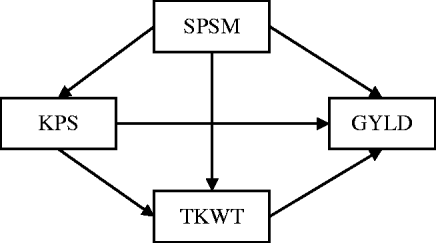
Fig. 1. The path diagram of the causal relationship among GRYL and yield components.
QTL-mapping studies are usually conducted for each trait separately using single trait analyses (Lander & Botstein, Reference Lander and Botstein1989; Haley & Knott, Reference Haley and Knott1992; Jansen & Stam, Reference Jansen and Stam1994; Zeng, Reference Zeng1994). However, such a single trait analysis may result in biased estimates and lower statistical power of QTL detection when data observations are collected on multiple causally related or genetically correlated traits. To combat these problems, several multiple trait QTL analysis (joint analysis) methods have been developed to take into account the correlation among multiple traits. These methods may be classified into multi-trait maximum-likelihood (ML) (Jiang & Zeng, Reference Jiang and Zeng1995; Williams et al., Reference Williams, Van Eerdewegh, Almasy and Blangero1999; Xu et al., Reference Xu, Li and Xu2005), multi-trait least squares (LS) (Calinski et al., Reference Calinski, Kaczmarek, Krajewski, Frova and Sari-Gorla2000; Knott & Haley, Reference Knott and Haley2000; Hackett et al., Reference Hackett, Meyer and Thomas2001), principal component analysis (PCA) (Weller et al., Reference Weller, Wiggans, Van Raden and Ron1996; Mangin et al., Reference Mangin, Thoquet and Grimsley1998) and discriminant analysis (DA) (Gilbert & Le Rol, Reference Gilbert and Le Roy2003). Multi-trait ML, implemented with the expectation conditional maximization (ECM) algorithm, provides a powerful tool to multi-trait QTL mapping. However, there are problems with this method when the number of QTLs and traits increase. The likelihood is a finite mixture of densities and becomes very difficult to evaluate (Satagopan et al., Reference Satagopan, Yandell, Newton and Osborn1996). The gains in power from joint analysis may compensate for the critical value for the test, due to the increase in the number of unknown parameters to be estimated (Mangin et al., Reference Mangin, Thoquet and Grimsley1998). Multi-trait LS, which regresses the quantitative trait value on the conditional expected genotypic value, produces results very similar to ML and simplifies computation (Haley & Knott, Reference Haley and Knott1992). The PCA and DA dimension reduction techniques, decompose the traits into a number of linear combinations that can be analysed separately. However, the approaches of PCA and DA may cause spurious linkages and difficulties in the biological interpretation of study results (Mähler et al., Reference Mähler, Most, Schmidtke, Sundberg, Li, Hedrich and Churchill2002; Gilbert & Le Roy, Reference Gilbert and Le Roy2003).
With new and powerful computational techniques available, Bayesian QTL mapping provides an extremely flexible way to search for multiple QTLs simultaneously. There are many practical advantages of using a Bayesian approach over frequentist approaches, such as the ability to fit more complex and biologically sensible models, the ability to incorporate prior information into the specification of the model, and the ability to obtain estimates of the posterior distributions of any function of the model parameters (Dunson, Reference Dunson2001; Yi & Shriner, Reference Yi and Shriner2008). The Bayesian approach has been extensively applied to QTL mapping for a single trait (Satagopan et al., Reference Satagopan, Yandell, Newton and Osborn1996; Sillanpaa & Arjas, Reference Sillanpaa and Arjas1998, Reference Sillanpaa and Arjas1999; Stephens & Fisch, Reference Stephens and Fisch1998; Yi & Xu, Reference Yi and Xu2002; Yi et al., Reference Yi, Xu and Allison2003, Reference Yi, Yandell, Churchill, Allison, Eisen and Pomp2005, Reference Yi, Shriner, Banerjee, Mehta, Pomp and Yandell2007; Narita & Sasaki, Reference Narita and Sasaki2004; Yi, Reference Yi2004; Wang et al., Reference Wang, Zhang, Li, Masinde, Mohan, Baylink and Xu2005). Recently, several Bayesian methods implemented via the Markov chain Monte Carlo (MCMC) algorithm have been developed for mapping multiple trait QTLs taking into account the correlation among traits. Meuwissen & Goddard (Reference Meuwissen and Goddard2004) combined linkage and linkage disequilibrium (LD) information to improve the power and precision of QTL mapping. Liu et al. (Reference Liu, Liu, Liu and Deng2007) developed a variance component method to model multiple complex traits in outbred populations using a Bayesian approach. In this approach, the number of QTLs is determined by reversible-jump MCMC (Green, Reference Green1995; Sillanpaa & Arjas, Reference Sillanpaa and Arjas1998). The problem with the reversible-jump MCMC for model selection is that it is usually subject to slow mixing of the Markov Chains and high computational demand associated with the algorithm (Wang et al., Reference Wang, Zhang, Li, Masinde, Mohan, Baylink and Xu2005). Yang & Xu (Reference Yang and Xu2007) extended the Bayesian shrinkage analysis (Wang et al., Reference Wang, Zhang, Li, Masinde, Mohan, Baylink and Xu2005) to dynamic complex traits by fitting the growth trajectory using Legendre polynomials. The advantage of this method is that it fits any trend in time but parameters of polynomials have no biological interpretation. Banerjee et al. (Reference Banerjee, Yandell and Yi2008) introduced the seemingly unrelated regression (SUR) model, which allows different genetic models for different traits. However, none are capable of dealing with the causal relationships among traits, resulting in the omission of the direct and indirect QTL effects.
The structural equation model (SEM) is a generalization of simultaneous equation procedures originating from path analysis (Wright, Reference Wright1921) and initially popularized in econometics and genetics. It is a useful method for estimating and evaluating simultaneous causal relationships among variables which allows variables to be both dependents and predictors. It is best explained by considering a path diagram. In particular, SEM allows researchers to decompose the effects of one variable on another into direct, indirect and total effects. The direct effect is the path coefficient between an independent variable and the dependent variable that are not causally explained by any other intermediary variable. The indirect effects of a variable are mediated by at least one other intervening variable. The indirect effects are calculated by multiplying the path coefficients for each path of the associated variable to the dependent variable. The total effect is the sum of direct and all indirect effects. By explicitly accounting for the complex multi-component causal structure among traits, SEM can provide a better understanding of multiple trait QTL analysis by allowing researchers to decompose the effects of one variable on another into direct, indirect and total effects within a QTL framework.
Recently, SEM has been applied to functionally related traits in genetic research with the goal of characterizing genetic architecture precisely and intuitively. Zhu & Zhang (Reference Zhu and Zhang2009) conducted simulation studies to compare the performance of multiple trait analysis and single trait analysis in family-based association studies. They found that multiple trait analysis improved the power of association tests and precision of parameter estimates when there are causal relations among the traits themselves. Nadeau et al. (Reference Nadeau, Burrage, Restivo, Pao, Churchill and Hoit2003) used the Bayesian network analysis to infer a functional/causal trait network of the cardiovascular system from a RIL population. Li et al. (Reference Li, Tsaih, Shockley, Stylianou, Wergedahl, Paigen and Churchill2006) analysed data from mouse inbred crosses to identify the causal networks including subphenotypes and QTL related to obesity and bone geometry. However, their approaches were limited to testing and quantifying the relationships among identified QTLs and phenotypes without QTL detection.
In this paper, we propose SEM in the context of QTL detection. The goal is to develop a Bayesian SEM approach mapping multiple traits QTL using recombinant inbred line (RIL) populations. The RIL populations are commonly used in QTL mapping experiments and are usually derived from a cross between two inbred parents followed by self-pollination and single-seed descent to reach homozygosity. The performance of the proposed method is evaluated by a simulation study and applied to data from a wheat experiment.
2. Statistical method
(i) Mixture SEM
Consider m QTLs located at positions λ1, λ2, …, λm in m different marker intervals I 1, I 2, …, Im in a linkage group on the same chromosome. Let the value of each marker and putative QTL be coded as 2 for one homozygous parent type and 0 with the other homozygous parent type, since the RILs are homozygous at every locus. Assume that p causally related quantitative traits y 1, y 2, …, and yp are affected by these m QTLs additively. The SEM in matrix form is
![\eqalign {\underbrace {\left[ {\matrix{ {y_{\setnum{1}} } \cr {y_{\setnum{2}} } \cr \vdots \cr {y_{p} } \cr} } \right]}_{\bf y} \equals \tab\underbrace {\left[ {\matrix{ 0 \tab {\beta _{\setnum{12}} } \tab \cdots \tab {\beta _{\setnum{1}p} } \cr 0 \tab 0 \tab \cdots \tab {\beta _{\setnum{2}p} } \cr \vdots \tab \vdots \tab \ddots \tab \vdots \cr 0 \tab 0 \tab \cdots \tab 0 \cr} } \right]}_{\bf B}\underbrace {\left[ {\matrix{ {y_{\setnum{1}} } \cr {y_{\setnum{2}} } \cr \vdots \cr {y_{p} } \cr} } \right]}_{\bf y} \plus \underbrace {\left[ {\matrix{ {\alpha _{\setnum{11}} } \cr {\alpha _{\setnum{12}} } \cr \vdots \cr {{\alpha} _{\setnum{1}p} } \cr} } \right]}_{{\bmalpha }_{\setnum{1}} } Q_{\setnum{1}}\cr\tab \plus \ldots \plus \underbrace {\left[ {\matrix{ {\alpha _{\setnum{21}} } \cr {\alpha _{\setnum{22}} } \cr \vdots \cr {\alpha _{\setnum{2}p} } \cr} } \right]}_{{\bmalpha }_{m} }Q_{m} \plus \underbrace {\left[ {\matrix{ {e_{\setnum{1}} } \cr {e_{\setnum{2}} } \cr \vdots \cr {e_{p} } \cr} } \right]}_{\bmzeta }\comma \quad\quad\quad\quad\quad\](https://static.cambridge.org/binary/version/id/urn:cambridge.org:id:binary:20160920235843672-0896:S0016672310000236:S0016672310000236_eqn1.gif?pub-status=live)
where yk is the phenotypic value for trait k (k=1, 2, …, p), βkh is the regression coefficient of trait h on trait k (h=1, 2, …, m), αlk is the direct effect of the lth putative QTL on trait k (l=1, 2, … , m), Ql is the lth putative QTL genotype, taking the value of 2 for genotype QQ and 0 for genotype qq and ek, the residual effect on trait k, is assumed to be multivariate normal distributed with means zero and covariance matrix

More compactly, the model (1) for ith individual (i=1, 2, …, n) can be rewritten as
and the reduced model
where yi is a p×1 vector of yk for the ith individual, B is the p×p coefficient matrix (contains βs) that describes causal relationship among p traits, where (I−B)−1 exists; αl is a p×1 vector of αlk, Qil is the putative QTL genotype for the lth QTL and ith individual; ζi, a p×1 vector of errors in the equation, is assumed to be multivariate and normally distributed with mean zero and diagonal covariance matrix Ψ. Elements in B, α=(α1, α2, …, αm) and Ψ are parameters that need to be estimated.
In practice, we observe the marker genotypes and trait values, but not the putative QTL genotypes. However, given the lth QTL positions λl and observed flanking marker genotypes, the distribution of the lth QTL genotype Ql in interval Il can be inferred in terms of the recombination frequency between them. We assume that there is no crossing-over interference. The conditional distributions of the individual putative QTL genotypes are independent given the flanking marker genotypes (Kao et al., Reference Kao, Zeng and Teasdale1999). The joint conditional probability of the genotype of the m putative QTL for individual i can be expressed as

where Qi is the joint QTL genotype for individual i; λ=(λ1, λ2, …, λm) are the locations of m QTLs; Ii=(Ii 1, Ii 2, …, Iim) are the intervals of flanking markers for individual i; Qil is the putative QTL genotype of the lth QTL for the ith individual. The joint conditional probability of the m QTL is the product of the marginal conditional probabilities of individual QTL. There are 2m possible different QTL genotypes in the population. We denote qij (j=1, 2, …, 2m) as the 2m possible QTL genotypes with the conditional probabilities of pij respectively for the ith individual, where pij containing information on QTL positions is non-negative and ![]() . That is, f(Qi=qij)=pij.
. That is, f(Qi=qij)=pij.
Given eqn (4), model (3) is defined as a finite mixture SEM. We assume the multivariate normal distribution of residual errors, the likelihood conditional on all unknowns λ=(λ1, λ2, …, λm), θ=(β’s, α1, α2, …, αm) and δ=(σ12, σ22, …,σp 2) is defined as

this is a 2m component mixture SEM, fj (yi|uj, Σ) is a multivariate normal density for the jth QTL genotype (j=1, 2, …, 2m) with probability pij, mean vector uj and a covariance matrix ![]() , assuming the same covariance matrix across all components. The mean vector ujs are derived from eqn (3) corresponding to the genotypic values of the 2m different QTL genotypes. For instance, in the two QTLs model, there are four multivariate normal densities with mean vectors
, assuming the same covariance matrix across all components. The mean vector ujs are derived from eqn (3) corresponding to the genotypic values of the 2m different QTL genotypes. For instance, in the two QTLs model, there are four multivariate normal densities with mean vectors ![]() , μ2=(I−B)−12α1, μ3=(I−B)−12α2 and μ4=0, respectively.
, μ2=(I−B)−12α1, μ3=(I−B)−12α2 and μ4=0, respectively.
The mean vectors and covariance matrix are functions of unknown parameters, which make the likelihood very difficult to evaluate by applying maximum likelihood procedures when the number of QTLs and traits increase. In response to this problem, we apply a Bayesian approach using an MCMC algorithm, which provides a powerful tool for solving complex mixtures. Inferences are based on the joint posterior distribution of all unknowns given the prior distribution of all unknowns and the observed data. We can also make use of posterior probability to obtain estimates of the posterior distributions of any function of the parameters, such as indirect and total QTL effects based on our proposed multi-trait SEM. The number of QTLs affecting traits is determined by the Bayes factor (BF).
Joint posterior distribution: in the Bayesian framework, the joint posterior distribution of all unknowns λ=(λ1, λ2, …, λm), θ=(β's, α1, α2, …, αm) and δ=(σ12, σ22, …, σp 2), given the trait values y, the marker genotypes (M) and prior information, can be expressed as

The terms f(y|Q, θ, δ)f(Q|λ) on the right-side of eqn (6) is the likelihood conditional on all unknowns, which is defined in eqn (5). The last term f(λ, θ, δ) is the joint prior distribution of all parameters (λ, θ, δ). We assume independence of prior distributions
The prior distribution of the QTL location λ is assumed to be uniform on a predefined interval. When no information regarding the locations is available, a prior uniform distribution with an interval equivalent to the length of the chromosome can be used. For convenience in elicitation and computation, we chose conjugate priors for the remaining parameters. The prior distribution of θ is assumed to be multivariate normal. The prior distributions of the variance component parameters are assumed to be independent inverse-gamma distributions.
Full conditional posterior distributions: from eqn (6) we can derive the full conditional posterior distributions.
The conditional distribution of a QTL genotype is

where fj (yi|uj, Σ) is a multivariate normal density function for the jth QTL genotype (j=1, 2, …, 2m) with mean vector uj and a covariance matrix ![]() . Let θ be a vector of the path coefficients (elements in α and B). The model (2)
. Let θ be a vector of the path coefficients (elements in α and B). The model (2) ![]() can be rewritten as
can be rewritten as ![]() , V(ζi)=Ψ, where yi is a p×1 vector of trait values for observation i (i=1, 2, …, n) with a known p×q matrix Ai containing yi and Qi; θ is a q×1 vector of coefficients to be estimated; ζi is a p×1 vector of random residuals, residual ζik is assumed to be uncorrelated and have variance
, V(ζi)=Ψ, where yi is a p×1 vector of trait values for observation i (i=1, 2, …, n) with a known p×q matrix Ai containing yi and Qi; θ is a q×1 vector of coefficients to be estimated; ζi is a p×1 vector of random residuals, residual ζik is assumed to be uncorrelated and have variance
θ and σk2 are assumed to follow the conjugate priors
The expected value γ*, covariance matrix Ωγ, e and f are chosen by the researcher. Arminger & Muthén (Reference Arminger and Muthén1998) suggested that one may set γ* to vector {1, …, 1}, Ωγ−1 to a diagonal matrix with small values, such as 0·01, set e to ½, and set f −1 to a small value, for instance 0·01. The posterior distribution of θ and σk2 is given as the following (Arminger & Muthén, Reference Arminger and Muthén1998):
![\eqalign {{\bmtheta }\vert {\bf y}\comma Q\comma {\bmPsi } \sim {\rm MVN} \tab \left( {\left( {\left[ {\mathop \sum\limits_{i \equals \setnum{1}}^{n} {{\bf A}_{i}}{\!\!\prime}\, {\bmPsi }^{ \minus \setnum{1}} {\bf A}_{i} } } \right] \plus \rmOmega _{\gamma }^{ \minus \setnum{1}} } \right)^{ \minus \setnum{1}} }\right\cr \tab\times{ \left( {\left[ {\mathop \sum\limits_{i \equals \setnum{1}}^{n} {{\bf A}_{i}{\!\!\prime}\, {\bmPsi }^{ \minus \setnum{1}} {\bf y}_{i} } } \right] \plus \rmOmega _{\gamma }^{ \minus \setnum{1}} \gamma \ast } \right)\comma } \cr \tab\left( {\left[ {\mathop\sum\limits_{i \equals \setnum{1}}^{n} {{\bf A}_{i}{\!\!\prime}\, {\bmPsi }^{ \minus \setnum{1}} {\bf A}_{i} } }\right] \plus \rmOmega _{\gamma }^{ \minus \setnum{1}} } } \right)^{ \minus \setnum{1}} \bigg)\comma\ \quad \!\!](https://static.cambridge.org/binary/version/id/urn:cambridge.org:id:binary:20160920235843672-0896:S0016672310000236:S0016672310000236_eqn9.gif?pub-status=live)
![\eqalign {\sigma _{k}^{\setnum{2}} \vert {\bf y}\comma Q\comma {\bmtheta } \sim \tab{\rm InvGamma}\left( {{n \over 2} \plus e\comma }\right \cr \tab\! \left[ {{1 \over 2}\mathop\sum\limits_{i \equals \setnum{1}}^{n} {\lpar y_{ik} \minus {\bf A}_{i} {\bmtheta }\rpar } \prime \lpar y_{ik} \minus {\bf A}_{i} {\bmtheta }\rpar \plus f^{ \minus \setnum{1}} } \right]^{ \minus \setnum{1}}\bigg ).}](https://static.cambridge.org/binary/version/id/urn:cambridge.org:id:binary:20160920235843672-0896:S0016672310000236:S0016672310000236_eqn10.gif?pub-status=live)
Based on fitting of the multi-trait SEM and posterior distribution of the path coefficients θ, we can obtain estimates of the posterior distributions of the indirect and total QTL effects, which are functions of θ. Unlike the above parameters θ and σk2, there is no explicit expression for the full conditional posterior distributions of the parameters λ. The Metropolis–Hastings sampler can be used to draw the samples from the joint posterior distribution (see detailed description in the following section).
(ii) Parameter estimate
Once all the full conditional posteriors are specified, the following MCMC algorithm can implemented.
Step 1. Initialization: Set the initial values of (λ(0), θ(0) and δ(0)) in the space of each parameter.
Step 2. Update the QTL position (λ): There is no closed form for the conditional posterior probability density of a QTL position. Therefore, we take the Metropolis–Hastings (Metropolis et al., Reference Metropolis, Rosenbluth, Rosenbluth, Teller and Teller1953; Hastings, Reference Hastings1970) approach for sampling the position of a QTL. Elements of λ are updated one at a time sequentially. Specifically, for the lth QTL, a proposal position λl* is sampled from a uniform distribution with symmetric interval (max (λl −1, λl−d), min(λl+d, λl +1)) around the previous position λl, where d is the predefined tuning parameter, usually taking a value of 2 cM. The proposed position λl* is accepted with probability.
where λ−l represents all elements of λ except λl. If the new position is accepted, the joint conditional probabilities (pij=f(Qi=qij|λ)) of the m QTL genotypes (see eqn (4)) is also updated simultaneously. Otherwise, the state remains unchanged, and the algorithm proceeds to update the next QTL position. The QTL position can be updated more than once between updates of other parameters if there is evidence that the chain is mixing slowly (Satagopan et al., Reference Satagopan, Yandell, Newton and Osborn1996).
Step 3. Update QTL genotype (Q): The genotype of joint m putative QTLs (Qi) is updated one individual at a time. It is sampled from its full conditional probability distribution (8)
Step 4. Update the path coefficients (θ): Elements of θ are simultaneously sampled from their full conditional distribution π(θ|λ, δ, Q, y) given in eqn (9), which is a multivariate normal distribution.
Step 5. Update the residual variances (δ): Elements in δ are updated individually based on their full conditional distribution f(σk2|λ, θ, σ−k2, Q, y) given in eqn (10), which is an inverted-gamma distribution.
Step 6. Update the indirect and total QTL effects: The indirect and total QTL effects are functions of the path coefficients θ. They are updated based on the current values of θ. The indirect QTL effect for a particular indirect path from the QTL to the trait is calculated by multiplying all the coefficients in the path. The total indirect QTL effect on the trait is the sum of all the indirect effects from all indirect paths.
Continued sampling by repeating steps 2–6 is known as the MCMC method, because the previous sample values are used as parameters to sample the next values, generating a Markov chain. When the chain is long enough, it converges to the stationary distribution; the sampled parameters actually follow the joint posterior distribution. Likewise, a sample of any single parameter is drawn from its marginal posterior density. Parameters can be estimated based on the samples from the corresponding posterior distributions. Here, we use the posterior mean as the Bayesian estimate.
(iii) Number of QTLs
We use the BF criterion (Jeffreys, Reference Jeffreys1961; Kass & Raftery, Reference Kass and Raftery1995) as a test statistic to detect QTLs. Specifically, this is the comparison of two different models with different number of QTLs affecting the traits using BFs. Let model1 and model0 be two competing models for a given data set. From Bayes theorem, the BF is defined as
The marginal probability of the data under modelj f(y|modelj) can be estimated using its harmonic mean estimator (Newton & Raftery, Reference Newton and Raftery1994).
where N is the number of total iterations in the MCMC process; λt, θt, δt, Qt are samples of all unknowns drawn from the tth iteration. Unlike the significance test approach that is based on P-values, this comparison does not depend on the assumption that either model is ‘true’, and can be applied to non-nested models. It is useful to consider the natural logarithm of the BF and interpret the resulting statistic based on the following criterion given by Kass & Raftery (Reference Kass and Raftery1995) : a negative log B 1−0 is taken as support for model0, while a value between 1 and 3 indicates support for model1 and a value in excess of 3 points to strong support for model1; a value between 0 and 1 does not allow any conclusion to be drawn.
3. A simulation study
The Bayesian analysis for multi-trait QTL mapping described above was investigated using simulation experiments. The data were simulated for 100 replicates of 250 lines from an RIL population. On a single chromosome segment of length 100 cM, 11 evenly spaced markers were simulated. Two QTLs (Q 1 and Q 2) were placed at 42 and 78 cM to affect three traits, which are causally related as in Fig. 2. The phenotypic values for each individual are determined by eqn (15), the causal relationship among the traits, the effects of two QTLs sampled (where QTL takes values of 2 and 0 for genotype QQ and qq, respectively) and the random residual effects were sampled from the multivariate normal distribution with mean zero and covariance matrix (16).
![\eqalign {\left[ {\matrix{ {y_{\setnum{1}} } \hfill \cr {y_{\setnum{2}} } \hfill \cr {y_{\setnum{3}} } \hfill \cr} } \right] \equals \tab\left( {\matrix{ 0 \tab {0{\cdot}5} \tab {0{\cdot}25} \cr 0 \tab \hskip -7pt0 \tab { \hskip -16pt\minus 0{\cdot}5} \cr 0 \tab \hskip -7pt0 \tab \hskip -13pt0 \cr} } \right) \left[ {\matrix{ {y_{\setnum{1}} } \cr {y_{\setnum{2}} } \cr {y_{\setnum{3}} } \cr} } \right] \plus \left[ {\matrix{ { \minus 0{\cdot}125} \cr {0{\cdot}5} \cr {\hskip 5pt0{\cdot}25} \cr} } \right]Q_{\setnum{1}} \cr \tab\plus \left[ {\matrix{ {\hskip 1pt0{\cdot}25} \cr { \hskip -14pt\minus 0{\cdot}5} \cr {\hskip -4pt \minus 0{\cdot}125} \cr} } \right]Q_{\setnum{2}} \plus \left[ {\matrix{ {\epsi _{\setnum{1}} } \cr {\epsi _{\setnum{2}} } \cr {\epsi _{\setnum{3}} } \cr} } \right]\comma \quad\quad\quad\quad\quad\quad\ \,](https://static.cambridge.org/binary/version/id/urn:cambridge.org:id:binary:20160920235843672-0896:S0016672310000236:S0016672310000236_eqn15.gif?pub-status=live)

A total of 100 replicates were analysed to study the variation across different generated samples and to estimate the power of QTL detection. Rather than using subsampling which is inefficient in comparison with full sampling (MacEachern & Berliner, Reference MacEachern and Berliner1994), we used the full Gibbs sample. For each of the MCMC analyses, the first 500 samples (burn-in) were discarded and an additional 2000 Gibbs samples from which parameters of the posterior distribution were estimated. There was evidence that the M-H chain for QTL position chain was mixing slowly. We tried a different number of M-H cycles to check the convergence (Arminger & Muthén, Reference Arminger and Muthén1998), and 25 cycles yielded satisfactory results in all simulations performed.
Single trait Bayesian analysis was also applied to the simulated data to compare the precision and efficiency with our proposed method. However, the single-trait method only estimates the total QTL effect on each trait, which is the sum of direct and indirect QTL effects. With the multi-trait SEM, the estimates of direct, indirect and total QTL effects are provided.
Models with different numbers of QTLs are compared, and the best one is selected based on the commonly used selection criterion BF. We compared the following models: (1) there is no QTL (model0) versus there is one QTL (model1), (2) there is one QTL (model1) versus there are two QTLs (model2) and (3) there are two QTLs (model2) versus there are three QTLs (model3). For all MCMC analyses, the same initial values and priors were used. The initial values for the QTL locations were set as 50 cM for model1, as 49 and 74 cM for model2, as 45, 74 and 89 cM for model3. The prior distribution for QTL locations was uniform over the chromosome. The tuning parameter of the proposal distribution for QTL locations was chosen to be 2·0 cM. The starting values were set as 0·1 for all regression parameters. The priors for the regression parameters were normally distributed with mean 1 and variance 100. The priors for the residual variances were inverse gamma (InvGamma(0.5,100)). All of the QTL models were fit for each of the 100 simulated data using the same chain length and burn-in.
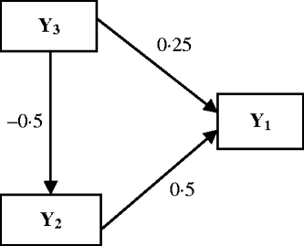
Fig. 2. Causal relationships among three traits in the simulation. Numbers by the arrow lines represent the true path coefficients.
4. Results
The estimated natural logarithm of the BFs (log(BF)s) for comparing different QTL models, averaged over 100 replicates, are given in Table 1. The average log(BF) comparing model0 versus model1 was −5·79 (against no QTL model 97 times out of 100 simulated datasets). The average log(BF) comparing model1 versus model2 was −23·56 with evidence in favour of two QTL model 99% of the times. An average log(BF) of 4·37 comparing model2 versus model3 favoured two QTL model 87% of the times. Therefore, it is concluded that the two QTL model was selected as the best fitting model. This conclusion is consistent with the simulated number of QTLs.
Table 1. BFs (using harmonic mean estimator) for multi-trait QTL-mapping model selection

Model0, Model1, Model2 and Model3 are the models with zero, one, two and three QTLs, respectively. Estimates are average over 100 replicates.
Now we restrict our attention to the two QTL model (model2). The approximate posterior distributions for the QTL locations are presented in Fig. 3. The graphs are symmetric and concentrated around the true simulated values.
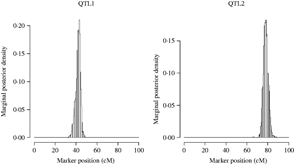
Fig. 3. Approximate posterior distribution of the QTL position in the simulation. The true number of QTL is two, located at position 42 and 78 cM.
The statistical power was determined by the proportion of the number of replicates in which the QTL was ‘detected’ over the total number of replicates. A QTL was claimed as detected if there was an obvious peak around the true simulated position. The overall power of single-trait analysis was calculated as the proportion of times the QTL was detected for at least one of the three traits. The power of detecting both simulated QTLs was calculated as the proportion of the number of replicates in which both QTLs were detected over the total number of replicates. The estimated QTL detection powers over 100 replicates are given in Table 2 by multi-trait SEM and single-trait Bayesian mapping methods. The QTL detection powers of the multi-trait SEM analysis were higher than those of the single-trait analysis for both QTLs. This result likely happened, because the single-trait method only estimates the total QTL effects which may be reduced, due to the compensating direct and indirect QTL effects. For instance, the QTL1 had a larger positive direct effect on Y2 but a negative indirect effect, which in turn reduces the total QTL effect on Y2. The relatively small total QTL effects associated with Y1, Y2 and Y3 may not be detected using single trait analysis. Based on the power analysis, the multi-trait SEM improved power of detecting individual QTL and both QTLs over the single trait analysis. However, the power of QTL detection may not necessarily always be higher for the multi-trait SEM than that for the single-trait analysis. If the direct and indirect QTL effects are in the same direction for all traits, the total QTL effect will be larger than the direct effects tested with the multi-trait SEM approach. In this case, the power of the multi-trait analysis may be less than the overall power of single-trait analysis since the single-trait method tests the total QTL effect. However, SEM can estimate indirect effects of any path which is not possible with the single-trait approach.
Table 2. Observed powers (%) of QTL detection of two methods obtained from 100 replicates in the simulation study
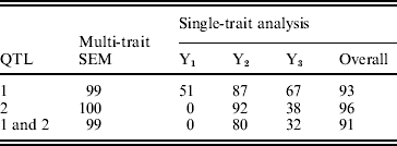
Figure 4 shows the Bayesian estimates of path coefficients with multi-trait SEM at the positions where the QTLs were detected. The estimated path coefficients are very close to the true simulated values. Table 3 presents the summary results of Bayesian parameter estimates in the simulation using our proposed method and the single-trait analysis. The means and standard deviations of the posterior distributions of the individual parameters are the averages over the 100 Monte Carlo replications. The estimates of QTL positions and effects by the multi-trait SEM method are very close to the true simulated values with small standard errors. However, the single-trait analysis provided estimates that appear to be biased with much higher standard deviations when compared with multi-trait SEM. The differences between two methods are especially large for QTLs with small total effects. Thus, multi-trait SEM method is more accurate and precise than single-trait analysis on the estimates of QTL positions and effects. Another obvious difference between our proposed method and the single-trait analysis is that multi-trait SEM allows one to fit a more complex and biologically sensible model, which provides the estimation of direct and indirect QTL effects, and therefore important insight giving a richer understanding of the nature of QTLs affecting traits compared with the single-trait analysis.
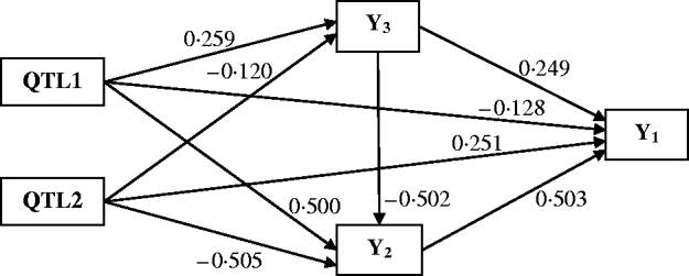
Fig. 4. Path model of multi-trait SEM in the simulation. Single arrows indicate causal relationships. Numbers by the arrow lines represent the Bayesian estimates of the path coefficients.
Table 3. Bayesian estimates of QTL positions and additive effects in the simulation by multi-trait SEM and single-trait analysis
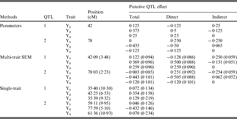
Estimates are means over 100 replications with standard deviation in parentheses. Sample size=250, Gibbs: Cycles=2000, Burn in=500 Metropolis: Cycles=25.
5. Application to recombinant inbred chromosome line (RICL) wheat experiment
We illustrate our Bayesian multi-trait SEM approach with an analysis of data from a RICLs wheat experiment, which contains a population of 98 RICLs-3A derived from a cross between ‘Cheyenne’ (CNN) and CNN with a ‘Wichita’ 3A chromosome substitution (CNN(WI3A)) and thus, the lines differed only in the which portion of ‘Wichita’ chromosome 3A was contained in each line. This population was evaluated in multi-environment field trials from 1999 to 2001 to identify QTL and QTL-by-environment interactions for GRYL and other agronomic traits in seven environments. Details of the experiment and results of the data analysis performed by univariate QTL detection techniques have been described by Campbell et al. (Reference Campbell, Baenziger, Gill, Eskridge, Budak, Erayman and Yen2003). These data were also analysed for genotype-by-environment interaction using a least squares SEM (Dhungana et al., Reference Dhungana, Eskridge, Baenziger, Campbell, Gill and Dweikat2007).
In this study, we focused on GYLD and yield component traits (TKWT, SPSM and KPS), since the causal relationships among these traits (Fig. 1) are well established (Dofing & Knight, Reference Dofing and Knight1992). To illustrate MCMC, we only considered 10 molecular markers covering 71·7 cM of the chromosome 3A in which two QTL regions were detected by Campbell et al. (Reference Campbell, Baenziger, Gill, Eskridge, Budak, Erayman and Yen2003). Prior to the analysis, analysis of variance (ANOVA) was performed for each trait to remove the main effects of environments and blocks. Residuals of the four traits were standardized to mean 0 and variance 1, and then were used as observed trait values.
We evaluated the one QTL model against the two QTL model and the two QTL model against the three QTL model using the BF. The prior distributions for the locations and additive effects of QTL, and other path coefficients were set to be the same as those in the simulation. The length of the Markov chain was also set to be the same as that in the simulation. The estimate of log(BF) of comparing one versus two QTL models was −39·15. Comparing the two versus three QTL models gave a log(BF) of 11·44, providing decisive evidence in favour of the two QTL model. Thus, the two QTL model was selected as the best-fitting model.
Figure 5 shows the marginal posterior probability distributions of the QTL locations obtained from the MCMC of the two QTL model. The first QTL is estimated at 5·31 cM (between Xbcd907 and Xtam055), affecting TKWT, KPS and SPSM directly. The second one is estimated at 56·1 cM (between markers XkusA6 and Xbcd366) affecting GYLD, KPS and SPSM directly.
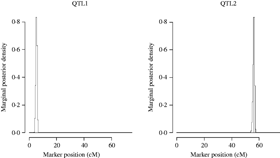
Fig. 5. Two QTL model. Approximate posterior distribution of two QTL locations based on joint analysis (multi-trait SEM) for GRYL and yield components on chromosome 3A of wheat.
Figure 6 shows the standardized path coefficients with multi-trait SEM located at two QTL locations. Table 4 shows the estimated posterior means and posterior standard deviations for the direct, indirect and total QTL effects of the identified QTLs. The QTL detected at position 5·3086 cM (close to Xbarc12) has a small positive direct effect (not significant) and a significant positive indirect effect on trait GYLD resulting in a large significant total QTL effect on trait GYLD. The direct and indirect QTL effects on TKWT are both negative (P<0·001) resulting in a large negative total effect (P<0·001), which significantly decreases TKWT. The QTL has a large positive direct effect on KPS (P<0·001) and a negative indirect effect (P<0·001) resulting in a smaller absolute total effect. The second QTL detected at position 56·01 cM (close to Xbarc67) affects all traits directly or indirectly. The direct and indirect QTL effects on GYLD are both positive (P<0·001) leading to a large total effect (P<0·001), which significantly increases GYLD. The QTL has significant negative indirect effects on both TKWT and KPS, but positive direct effects leading to non-significant total effects, since the direct and indirect effects are cancelled out. In contrast, in their combined analysis Campbell et al. (Reference Campbell, Baenziger, Gill, Eskridge, Budak, Erayman and Yen2003) were not able to detect QTLs for SPSM in either region using univariate QTL detection techniques which only captured the total QTL effects. In addition, they detected a minor QTL for GYLD in region one, while the corresponding QTL that we detected had a greater effect on GYLD. Thus, by considering the GRYL and yield components together in a multi-trait analysis, we not only improved the ability to detect QTLs for GYLD and SPSM but also gained insight into the processes of how the QTLs on chromosome 3A affected agronomic performance directly and indirectly. Understanding the genetic control of GRYL using a biologically relevant yield component framework provides useful information for plant breeders interested in breaking unfavourable indirect QTL effects and for better understanding complex traits.
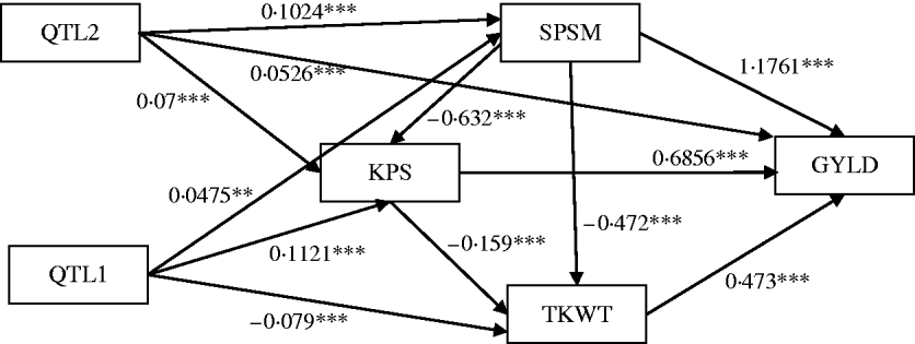
Fig. 6. Path estimates of multi-trait SEM at positions 5·3086 cM (QTL1, close to Xbarc12) and 56·005 cM (QTL2, close to Xbarc67) on chromosome 3A of wheat. Single arrows indicate causal relationships. Numbers by the arrow lines represent the estimated standardized coefficients with significance level: ***P<0·001, **P<0·01 and *P<0·05.
Table 4. Bayesian estimates of the chromosome 3A QTL locations and effects using multi-trait SEM

Values in parentheses are respective SD values.
6. Discussion and conclusion
Research on QTL studies often provides information on multiple complex traits that have well-established causal relationships. However, there has been a lack of a comprehensive multivariate multiple QTL-mapping technique which is capable of incorporating the causal structure among multiple traits. Consequently the genetic functions may not be fully understood. In this study, we have presented a Bayesian approach to multiple traits QTL mapping using an SEM, taking into account the causal relationships among multiple traits. We have explored some aspects of multiple traits QTL mapping that have not been done in previous studies. In particular, it allows one to fit a more complex and biologically sensible model; it provides the estimates of the total, direct and indirect QTL effects and ultimately allows for important insights into how QTLs regulate multiple complex traits. Knowledge of the direct and indirect QTL effects can be very important for plant breeders interested in finding modifier genes to overcome the pleiotropism.
Using our proposed multi-trait SEM, we were able to improve the power of QTL detection and precision of parameter estimates compared with the single-trait analysis. However, the power of the QTL detection may not necessarily always be higher for the multi-trait SEM. It depends on the magnitude of QTL effects and the directions of causal relationship among multiple traits. The power of the multi-trait SEM can increase significantly if the direct and indirect QTL effects on the trait are relatively large and in the opposite direction, which reduces the total QTL effect. In this case, the reduced total QTL may not be detected by the single-trait analysis since the single-trait method tests only the total QTL effect. If QTL influences traits that are not causally explained by any other intermediary trait, the power of multi-trait SEM is very close to that of the single-trait analysis since the direct and total QTL effects are the same. If the direct and indirect QTL effects are in the same direction for the trait, the total QTL effect will be larger than the direct effects tested with the multi-trait SEM approach. In this case, the power of the multi-trait SEM analysis may be less than the overall power of single-trait analysis.
We also applied Bayesian multi-trait SEM to the RICLs-3A wheat experiment data. As expected, we detected QTLs for SPSM in either region which have not been reported in Campbell et al. (Reference Campbell, Baenziger, Gill, Eskridge, Budak, Erayman and Yen2003), where univariate QTL detection techniques were used. In addition, they detected a minor QTL for GYLD in region one, while the corresponding QTL that we detected had a greater effect on GYLD.
A prerequisite of the proposed method is prior biological knowledge of the causal relationships among the multiple traits, since SEM is generally used as a confirmatory rather than exploratory procedure. Theoretical insight and judgment by the researcher is very important in building a correct model. In practice, one can obtain some basic background about the key structure of the model either from knowledge of the related field or from preliminary data analyses. Other applications likely may require more model development based on procedures described elsewhere (see Bollen, Reference Bollen1989).
The model considered in this paper was illustrated using an RIL-simulated population to provide a general idea of the nature of QTLs affecting the traits, and did not include epistatic genetic effects. However, the general approach can be easily applied to different population structures (such as F2 and backcross), and genetic models by setting up the corresponding conditional QTL genotype probability given QTL locations. Here, we assumed a pleiotropic QTL model (each QTL affects all traits). It is important to separate pleiotropic effects against closely linked QTL. We plan to use BF to test pleiotropic effects against closely linked QTL in the future. In this study, we assumed complete phenotypic data. However, we acknowledged that a large amount of missing phenotypic data may reduce the power of QTL detection and precision of QTL location and effect estimation in joint analyses (Fridley & de Andrade, Reference Fridley and de Andrade2008; Guo & Nelson, Reference Guo and Nelson2008). Our proposed method can be extended to deal with missing phenotypic data by using multiple imputations. The proposed model here did not account for the experimental design issue, thus ignoring non-genetic sources of variation such as environments, blocks or gene–environment interactions. Methods incorporating these innovations could result in increased statistical power of QTL detection, precision in estimation of QTL effects and position and an improved understanding of how QTL interact with environmental factors. In addition, researchers may collect data of different types for a sample set (e.g. both binary and continuous traits). Methods that are capable of dealing with a mixture of continuous and binary traits could be valuable in a variety of situations.
Programs were written in SAS PROC IML and are available by sending email to [email protected]


