


1. Introduction
Wave turbulence theory (WTT) provides the statistical description of the evolution of the wave action spectral density of a weakly nonlinear interacting system of a large number of waves (Zakharov et al. Reference Zakharov, L’vov and Falkovich2012, Newell & Rumpf Reference Newell and Rumpf2011, Nazarenko Reference Nazarenko2011, Galtier Reference Galtier2022). The central object of the theory is the wave kinetic equation (WKE), first introduced by Peierls (Reference Peierls1929), which is the analogue for a system of interacting waves of Boltzmann’s kinetic equation for particles in a rarefied gas Cercignani (Reference Cercignani1988). For surface gravity waves, the WKE was derived by Hasselmann (Reference Hasselmann1962) and Zakharov & Filonenko (Reference Zakharov and Filonenko1967a ), and it is currently the building block of wave operational models (Komen et al. Reference Komen, Cavaleri, Donelan, Hasselmann, Hasselmann and Janssen1996, Cavaleri et al. Reference Cavaleri2007).
Although its rigorous derivation (in a mathematical sense, establishing the convergence of the asymptotic expansion) has been proved only for the nonlinear Schrödinger equation in dimensions larger than one (see Deng & Hani Reference Deng and Hani2023a,b ), in the past decades the WKE has been derived (without a rigorous mathematical proof) and widely used in various systems such as internal gravity waves (Olbers Reference Olbers1976; Caillol & Zeitlin Reference Caillol and Zeitlin2000; Lvov & Tabak Reference Lvov and Tabak2004), capillary waves (Zakharov & Filonenko Reference Zakharov and Filonenko1967b ), surface waves (Hasselmann Reference Hasselmann1962; Krasitskii Reference Krasitskii1994; Zakharov (Reference Zakharov1999), plasma waves in magnetohydrodynamics (Galtier et al. Reference Galtier, Nazarenko, Newell and Pouquet2000,Kuznetsov Reference Kuznetsov2001, Bose–Einstein condensation (Lvov et al. Reference Lvov, Nazarenko and West2003,Nazarenko & Onorato Reference Nazarenko and Onorato2006), gravitational waves (Galtier & Nazarenko Reference Galtier and Nazarenko2021) and vibrating plates (Düring et al. Reference Düring, Josserand and Rica2006,Cobelli et al. Reference Cobelli, Petitjeans, Maurel, Pagneux and Mordant2009). In real systems, dissipation cannot be neglected. For example, experiments in elastic plates revealed a discrepancy between theoretical predictions on Kolmogorov–Zakharov spectra (Düring et al. Reference Düring, Josserand and Rica2006) and experimental results (Boudaoud et al. Reference Boudaoud, Cadot, Odille and Touzé2008,Mordant Reference Mordant2010). Among all the reasons for which these discrepancies can arise, Humbert et al. (Reference Humbert, Cadot, Düring, Josserand, Rica and Touzé2013) proposed that the origin of the mismatch is due to dissipation, which is inevitably present in all elastic plates. For surface gravity waves, dissipation due to white capping or wave breaking also plays an important role in the dynamics, and different models have been developed and phenomenologically included in the energy balance equation (Ardhuin et al. Reference Ardhuin2010,Babanin Reference Babanin2011,Komen et al. Reference Komen, Cavaleri, Donelan, Hasselmann, Hasselmann and Janssen1996,Liu et al. Reference Liu, Rogers, Babanin, Young, Romero, Zieger, Qiao and Guan2019,Cavaleri et al. Reference Cavaleri2007). In WTT, the dissipative effects, as well as the external forcing are added a posteriori only after the WKE has been derived for conservative dynamics. However, in principle, dissipation and forcing may play a role combined with resonant interactions. Therefore, it is important to build a framework in which dissipation and forcing are taken into account starting from deterministic equations of motion.
In this paper, we consider this possibility and provide a derivation of the WKE, assuming the presence of dissipation/forcing in the deterministic governing equations (in the form of the so-called Zakharov equation). More specifically, we assume that our system is characterised by two small parameters,
 $\epsilon$
and
$\epsilon$
and
 $\mu$
; the former is related to the strength of the nonlinear interactions and the latter to dissipation/forcing. We emphasise that, although in the literature
$\mu$
; the former is related to the strength of the nonlinear interactions and the latter to dissipation/forcing. We emphasise that, although in the literature
 $\epsilon$
usually denotes the wave steepness, throughout this manuscript,
$\epsilon$
usually denotes the wave steepness, throughout this manuscript,
 $\epsilon$
represents the square of the steepness. In this paper, we consider two different scalings between the two parameters: the first is when the dissipation/forcing acts on the kinetic time scale
$\epsilon$
represents the square of the steepness. In this paper, we consider two different scalings between the two parameters: the first is when the dissipation/forcing acts on the kinetic time scale
 $\mu \sim \epsilon ^{2}$
, which is the time scale of the four-wave resonances, while the second case of study is when the dissipation/forcing acts on an intermediate time scale
$\mu \sim \epsilon ^{2}$
, which is the time scale of the four-wave resonances, while the second case of study is when the dissipation/forcing acts on an intermediate time scale
 $\mu \sim \epsilon$
.
$\mu \sim \epsilon$
.
2. The Zakharov equation with dissipation/forcing
Throughout the manuscript, we consider a physical domain
 $[0,L]\times [0,L]$
, which implies a two-dimensional infinite discrete Fourier space. The spacing in Fourier space is given by
$[0,L]\times [0,L]$
, which implies a two-dimensional infinite discrete Fourier space. The spacing in Fourier space is given by
 $\Delta k = 2\pi /L$
. We use the following notation:
$\Delta k = 2\pi /L$
. We use the following notation:
 \begin{equation} \sum _{1234}\equiv \sum _{{\boldsymbol k}_1, {\boldsymbol k}_2, {\boldsymbol k}_3, {\boldsymbol k}_4},\quad \delta _{12}^{34}\equiv \delta _{{\boldsymbol k}_1+ {\boldsymbol k}_2, {\boldsymbol k}_3+ {\boldsymbol k}_4} \enspace \text { is the Kronecker delta,} \end{equation}
 \begin{equation} X_{i}\equiv X_{{\boldsymbol k}_i},\qquad \Delta X_{12}^{34}\equiv X_{1}+X_{2}-X_{3}-X_{4}\enspace \text { for any variable X,} \end{equation}
and the summation goes from
 $-\infty$
to
$-\infty$
to
 $+\infty$
. It is well known that, under the hypothesis of inviscid and irrotational flow, in the limit of weak nonlinearity, the Euler equations for water waves reduce to the Zakharov equation (Stuhlmeier Reference Stuhlmeier2024; Krasitskii Reference Krasitskii1994). In the presence of dissipation, we assume that the Zakharov equation, written in terms of the normal variable
$+\infty$
. It is well known that, under the hypothesis of inviscid and irrotational flow, in the limit of weak nonlinearity, the Euler equations for water waves reduce to the Zakharov equation (Stuhlmeier Reference Stuhlmeier2024; Krasitskii Reference Krasitskii1994). In the presence of dissipation, we assume that the Zakharov equation, written in terms of the normal variable
 $a_{\mathbf {k}}$
, is corrected by an extra term and takes the form
$a_{\mathbf {k}}$
, is corrected by an extra term and takes the form
 \begin{equation} {\rm{i}}\frac {\textrm {d} a_1}{\textrm {d} t}=\omega _1a_1+\epsilon \sum _{234} T_{1234}a^*_2a_3a_4\delta _{12}^{34}-{\rm{i}}\mu \gamma _1 a_1, \end{equation}
where
 $\omega _k=\sqrt {g k \tanh (kh)}$
is the dispersion relation,
$\omega _k=\sqrt {g k \tanh (kh)}$
is the dispersion relation,
 $k=\vert {\boldsymbol k} \vert$
and
$k=\vert {\boldsymbol k} \vert$
and
 $h$
is the water depth. Although
$h$
is the water depth. Although
 $h$
can be arbitrary, caveats have to be considered in the limit of shallow water in which the system becomes non-dispersive and lacks the natural randomisation of phases, fundamental for the derivation of the WKE. The matrix elements that weight the interactions,
$h$
can be arbitrary, caveats have to be considered in the limit of shallow water in which the system becomes non-dispersive and lacks the natural randomisation of phases, fundamental for the derivation of the WKE. The matrix elements that weight the interactions,
 $T_{1234}$
, can be found in Krasitskii (Reference Krasitskii1990) or Janssen & Onorato (Reference Janssen and Onorato2007). The term
$T_{1234}$
, can be found in Krasitskii (Reference Krasitskii1990) or Janssen & Onorato (Reference Janssen and Onorato2007). The term
 $ \gamma _k a_k$
can be interpreted as a forcing or a dissipation; in general,
$ \gamma _k a_k$
can be interpreted as a forcing or a dissipation; in general,
 $\gamma _k$
is the sum of two contributions: a positive one that mimics the dissipation and a negative one that plays the role of forcing. The terms
$\gamma _k$
is the sum of two contributions: a positive one that mimics the dissipation and a negative one that plays the role of forcing. The terms
 $\epsilon$
and
$\epsilon$
and
 $\mu$
, both greater than zero, are the nonlinear and the dissipation/forcing coefficients, respectively. To avoid secular growths in the upcoming perturbation theory, we isolate the trivial resonances
$\mu$
, both greater than zero, are the nonlinear and the dissipation/forcing coefficients, respectively. To avoid secular growths in the upcoming perturbation theory, we isolate the trivial resonances
 ${\boldsymbol k}_1={\boldsymbol k}_2={\boldsymbol k}_3={\boldsymbol k}_4$
;
${\boldsymbol k}_1={\boldsymbol k}_2={\boldsymbol k}_3={\boldsymbol k}_4$
;
 ${\boldsymbol k}_1={\boldsymbol k}_3$
and
${\boldsymbol k}_1={\boldsymbol k}_3$
and
 ${\boldsymbol k}_2={\boldsymbol k}_4$
;
${\boldsymbol k}_2={\boldsymbol k}_4$
;
 ${\boldsymbol k}_1={\boldsymbol k}_4$
and
${\boldsymbol k}_1={\boldsymbol k}_4$
and
 ${\boldsymbol k}_2={\boldsymbol k}_3$
from the nonlinear term in (2.3). We reabsorb them as corrections to the linear oscillation. The Zakharov equation becomes
${\boldsymbol k}_2={\boldsymbol k}_3$
from the nonlinear term in (2.3). We reabsorb them as corrections to the linear oscillation. The Zakharov equation becomes
 \begin{align} {\rm{i}}\frac {\textrm {d} a_1}{\textrm {d} t}=\varOmega _1a_1+\epsilon \sum^{\prime }_{234} T_{1234}a^*_2a_3a_4\delta _{12}^{34}-{\rm{i}}\mu \gamma _1 a_1, \end{align}
where
 \begin{align} \varOmega _1=\omega _1+2\epsilon \sum _{2}T_{1212}|a_2|^2-\epsilon T_{1111}|a_1|^2 \end{align}
is the renormalised frequency, and the prime in the summation means that only the non-trivial interactions are considered. To derive the kinetic equation, we consider the method developed in Onorato & Dematteis (Reference Onorato and Dematteis2020); we emphasise that the results we obtain do not depend on the method used, and a check has also been carried out using a more standard expansion of the correlators, which confirms our results.
We introduce two real functions, the action
 $I_{\boldsymbol k}$
and the angle
$I_{\boldsymbol k}$
and the angle
 $\theta _{\boldsymbol k}$
, such that
$\theta _{\boldsymbol k}$
, such that
 \begin{equation} a_{\boldsymbol k}(t)=\sqrt {I_{\boldsymbol k}(t)}{\rm{e}}^{-{\rm{i}}\theta _{\boldsymbol k}(t)}. \end{equation}
By inserting (2.6) into (2.4), separating the imaginary and real parts, the equations for
 $I_{\boldsymbol k}$
and
$I_{\boldsymbol k}$
and
 $\theta _{\boldsymbol k}$
read
$\theta _{\boldsymbol k}$
read
 \begin{align} \frac {\textrm {d} I_1}{\textrm {d} t}&=2\epsilon \sum ^{\prime }_{234}T_{1234} \sqrt {I_1I_2I_3I_4}\sin (\Delta \theta _{12}^{34})\delta _{12}^{34}-2\mu \gamma _1 I_1, \end{align}
 \begin{align} \frac {\textrm {d} \theta _1}{\textrm {d} t}&=\varOmega _1+\epsilon \sum ^{\prime }_{234}T_{1234}\sqrt {\frac {I_2I_3I_4}{I_1}}\cos (\Delta \theta _{12}^{34})\delta _{12}^{34}, \end{align}
with initial conditions
 $I_1(0)=\bar {I}_1$
and
$I_1(0)=\bar {I}_1$
and
 $ \theta _1(0)=\bar {\theta }_1$
.
$ \theta _1(0)=\bar {\theta }_1$
.
3. The kinetic equation with dissipation/forcing
In the Zakharov equation with dissipation/forcing, the dispersion is considered to be a dominant term, whereas nonlinearity and dissipation/forcing are assumed to be small. In the absence of dissipation/forcing, it is well known that, for
 $\epsilon \ll 1$
, the time scale at which the kinetic equation becomes relevant is
$\epsilon \ll 1$
, the time scale at which the kinetic equation becomes relevant is
 $t\sim 1/\epsilon ^2$
. In the Zakharov equation with dissipation/forcing, we have the presence of two small parameters,
$t\sim 1/\epsilon ^2$
. In the Zakharov equation with dissipation/forcing, we have the presence of two small parameters,
 $\mu$
and
$\mu$
and
 $\epsilon$
(which are assumed to be small compared with the dispersive term). Different scalings can be considered: one possibility is that dissipation/forcing acts on the kinetic timescale
$\epsilon$
(which are assumed to be small compared with the dispersive term). Different scalings can be considered: one possibility is that dissipation/forcing acts on the kinetic timescale
 $\mu \sim \epsilon ^2$
, and the other case is when dissipation/forcing acts on an intermediate time scale,
$\mu \sim \epsilon ^2$
, and the other case is when dissipation/forcing acts on an intermediate time scale,
 $\mu \sim \epsilon$
. In the following, we investigate these two scenarios using the same approach developed in Onorato & Dematteis (Reference Onorato and Dematteis2020) with the appropriate modifications due to the presence of dissipation/forcing. (Note that, in Appendix D, we verify our final results using a more conventional approach based on the expansion of the correlators.)
$\mu \sim \epsilon$
. In the following, we investigate these two scenarios using the same approach developed in Onorato & Dematteis (Reference Onorato and Dematteis2020) with the appropriate modifications due to the presence of dissipation/forcing. (Note that, in Appendix D, we verify our final results using a more conventional approach based on the expansion of the correlators.)
3.1.
The dissipation/forcing acting on the kinetic time scale
 $\mu \sim \epsilon ^2$

3.1.1. Small-
$\epsilon$
perturbative expansion

We expand
 $I_{\boldsymbol k}$
and
$I_{\boldsymbol k}$
and
 $\theta _{\boldsymbol k}$
in powers of the nonlinear coefficient
$\theta _{\boldsymbol k}$
in powers of the nonlinear coefficient
 $\epsilon$
as follows:
$\epsilon$
as follows:
 \begin{align} I_{\boldsymbol k}&=I_{\boldsymbol k}^{(0)}+\epsilon I_{\boldsymbol k}^{(1)}+\epsilon ^2I_{\boldsymbol k}^{(2)}+\mathcal {O}(\epsilon ^3), \end{align}
 \begin{align} \theta _{\boldsymbol k}&=\theta _{\boldsymbol k}^{(0)}+\epsilon \theta _{\boldsymbol k}^{(1)}+\epsilon ^2\theta _{\boldsymbol k}^{(2)}+\mathcal {O}(\epsilon ^3), \end{align}
which can be inserted into (2.8) and (2.7), and we match powers of
 $\epsilon$
. Because the dissipation/forcing enters at order
$\epsilon$
. Because the dissipation/forcing enters at order
 $\epsilon ^2$
, the expansion up to order
$\epsilon ^2$
, the expansion up to order
 $\epsilon$
remains identical to the one presented in Onorato & Dematteis (Reference Onorato and Dematteis2020). Here, we report the main results.
$\epsilon$
remains identical to the one presented in Onorato & Dematteis (Reference Onorato and Dematteis2020). Here, we report the main results.
3.1.2. Order
$\epsilon ^0$
.

At order
 $\epsilon ^0$
, we find
$\epsilon ^0$
, we find
 \begin{equation} \frac {\textrm {d} I_1^{(0)}}{\textrm {d} t}=0,\qquad \frac {\textrm {d} \theta _1^{(0)}}{\textrm {d} t}=\varOmega _1, \end{equation}
which can be integrated from 0 to
 $t$
, leading to
$t$
, leading to
 \begin{equation} I_1^{(0)}(t)=\bar {I}_1,\qquad \theta _1^{(0)}(t)=\bar {\varOmega }_1 t+\bar {\theta }_1, \end{equation}
where the bar denotes the quantity evaluated at time
 $t=0$
.
$t=0$
.
3.1.3. Order
$\epsilon ^1$
.

At order
 $\epsilon$
, after inserting the results at order
$\epsilon$
, after inserting the results at order
 $\epsilon ^0$
, we obtain
$\epsilon ^0$
, we obtain
 \begin{align} \frac {\textrm {d} I_1^{(1)}}{\textrm {d} t}&=2\sum ^{\prime }_{234} T_{1234}\sqrt {\bar {I}_1\bar {I}_2\bar {I}_3\bar {I}_4}\sin (\Delta \bar {\theta }_{12}^{34}+\Delta \bar {\varOmega }_{12}^{34}t)\delta _{12}^{34}, \end{align}
 \begin{align} \frac {\textrm {d} \theta _1^{(1)}}{\textrm {d} t}&=\sum ^{\prime }_{234}T_{1234}\sqrt {\frac {\bar {I}_2\bar {I}_3\bar {I}_4}{\bar {I}_1}}\cos (\Delta \bar {\theta }_{12}^{34}+\Delta \bar {\varOmega }_{12}^{34}t)\delta _{12}^{34}, \end{align}
which can be integrated from 0 to
 $t$
, leading to
$t$
, leading to
 \begin{align} I_1^{(1)}(t)&=2\sum ^{\prime }_{234} T_{1234}\sqrt {\bar {I}_1\bar {I}_2\bar {I}_3\bar {I}_4} \frac {\cos (\Delta \bar {\theta }_{12}^{34})-\cos (\Delta \bar {\theta }_{12}^{34}+\Delta \bar {\varOmega }_{12}^{34}t )}{\Delta \bar {\varOmega }_{12}^{34}}\delta _{12}^{34}, \end{align}
 \begin{align} \theta _1^{(1)}(t)&=-\sum ^{\prime }_{234}T_{1234}\sqrt {\frac {\bar {I}_2\bar {I}_3\bar {I}_4}{\bar {I}_1}}\frac {\sin (\Delta \bar {\theta }_{12}^{34})-\sin (\Delta \bar {\theta }_{12}^{34}+\Delta \bar {\varOmega }_{12}^{34}t )}{\Delta \bar {\varOmega }_{12}^{34}}\delta _{12}^{34}. \end{align}
3.1.4. Order
$\epsilon ^2$
.

After inserting (3.7) and (3.8) in the expansions
 $I_{\boldsymbol k}(t)=\bar {I}_{\boldsymbol k}+\epsilon I_{\boldsymbol k}^{(1)}(t)$
and
$I_{\boldsymbol k}(t)=\bar {I}_{\boldsymbol k}+\epsilon I_{\boldsymbol k}^{(1)}(t)$
and
 $\theta _{\boldsymbol k}(t)=\bar {\theta }_{\boldsymbol k}+\bar {\varOmega }_{\boldsymbol k}t+\epsilon \theta _{\boldsymbol k}^{(1)}(t)$
, we substitute them into (2.7) and keeping terms at order
$\theta _{\boldsymbol k}(t)=\bar {\theta }_{\boldsymbol k}+\bar {\varOmega }_{\boldsymbol k}t+\epsilon \theta _{\boldsymbol k}^{(1)}(t)$
, we substitute them into (2.7) and keeping terms at order
 $\epsilon ^2$
gives
$\epsilon ^2$
gives
 \begin{align} \frac {\textrm {d} I_1^{(2)}}{\textrm {d} t}&=2\sum ^{\prime }_{\substack {234\\567}}\sum _{m=1}^4T_{1234}T_{m567}\frac {\sqrt {\bar {I}_1\bar {I}_2\bar {I}_3\bar {I}_4\bar {I}_5\bar {I}_6\bar {I}_7}}{\sqrt {\bar {I}_m}\Delta \bar {\varOmega }_{m5}^{67}}\delta _{12}^{34}\delta _{m5}^{67}\left \{ \sin (\Delta \bar {\theta }_{12}^{34}+\Delta \bar {\varOmega }_{12}^{34}t-\sigma _m \Delta \bar {\theta }_{m5}^{67}) \right . \nonumber \\ &\quad\left . + \sin \left [\sigma _m(\Delta \bar {\theta }_{m5}^{67}+\Delta \bar {\varOmega }_{m5}^{67}t)-\Delta \bar {\theta }_{12}^{34}-\Delta \bar {\varOmega }_{12}^{34}t\right ]\right \}-2\gamma _1\bar I_1, \end{align}
where
 $\sigma _m=\{+1,+1,-1,-1\}$
. The next step in the derivation of the kinetic equation is to perform averages on the distribution of the initial data. We assume that phases and actions are independent identically distributed random variables. More specifically, phases will be considered to be uniformly distributed, whereas for actions it is not necessary to specify any distribution (random phase and amplitude (RPA)) assumption, Nazarenko Reference Nazarenko2011). The procedure of averaging over the phases is described in Appendix (A); the first non-zero contribution is at second order and is given by
$\sigma _m=\{+1,+1,-1,-1\}$
. The next step in the derivation of the kinetic equation is to perform averages on the distribution of the initial data. We assume that phases and actions are independent identically distributed random variables. More specifically, phases will be considered to be uniformly distributed, whereas for actions it is not necessary to specify any distribution (random phase and amplitude (RPA)) assumption, Nazarenko Reference Nazarenko2011). The procedure of averaging over the phases is described in Appendix (A); the first non-zero contribution is at second order and is given by
 \begin{align} \frac {\textrm {d} \langle I_1\rangle _{\bar {\theta }}}{\textrm {d} t} = 4\epsilon ^2 \sum ^{\prime }_{234}T_{1234}^2 \bar {I}_1\bar {I}_2\bar {I}_3\bar {I}_4 \sum _{m=1}^4 \frac {\sigma _m}{\bar {I}_m} \frac {\sin (\Delta \bar {\varOmega }_{12}^{34}t)}{\Delta \bar {\varOmega }_{12}^{34}}\delta _{12}^{34}- 2\gamma _1\bar I_1. \end{align}
3.1.5. The large-box limit
So far, the calculation has been performed by assuming that, in physical space, the wave field is periodic in space with period
 $L$
; the derivation of the kinetic equation requires the large box limit, which is achieved by considering the limit
$L$
; the derivation of the kinetic equation requires the large box limit, which is achieved by considering the limit
 $L\to +\infty$
, and it corresponds to taking the distance between Fourier modes approaching zero. An additional step in the derivation of the kinetic equation is to evaluate the average over the initial actions which, by hypothesis, are assumed to be statistically independent, i.e.
$L\to +\infty$
, and it corresponds to taking the distance between Fourier modes approaching zero. An additional step in the derivation of the kinetic equation is to evaluate the average over the initial actions which, by hypothesis, are assumed to be statistically independent, i.e.
 $\langle \bar {I}_1\bar {I}_2\bar {I}_3\bar {I}_4\rangle _{\bar {I}}=\langle \bar {I}_1\rangle _{\bar {I}}\langle \bar {I}_2\rangle _{\bar {I}}\langle \bar {I}_3\rangle _{\bar {I}}\langle \bar {I}_4\rangle _{\bar {I}}$
. Therefore, we define the spectral action density
$\langle \bar {I}_1\bar {I}_2\bar {I}_3\bar {I}_4\rangle _{\bar {I}}=\langle \bar {I}_1\rangle _{\bar {I}}\langle \bar {I}_2\rangle _{\bar {I}}\langle \bar {I}_3\rangle _{\bar {I}}\langle \bar {I}_4\rangle _{\bar {I}}$
. Therefore, we define the spectral action density
 \begin{align} n_{\boldsymbol k}(t)=n({\boldsymbol k},t)=\lim _{\Delta k\to 0}\frac { \langle I_k\rangle _{\bar \theta ,\bar I}}{(\Delta k)^2}, \end{align}
and by following the standard rules for correspondence between sums and integrals, Kronecker’s delta and the Dirac delta,
 \begin{align} \sum _{\boldsymbol k}\longrightarrow \int \frac {\textrm {d} {\boldsymbol k}}{(\Delta k)^2},\qquad \delta _{12}^{34}\longrightarrow \delta (\Delta {\boldsymbol k}_{12}^{34})(\Delta k)^2, \end{align}
we obtain
 \begin{align} \frac {\partial n_1}{\partial \tau _2}=&4\int \textrm {d} {\boldsymbol k}_{234} T_{1234}^2\bar {n}_1\bar {n}_2\bar {n}_3\bar {n}_4\sum _{m=1}^4 \frac {\sigma _m }{\bar {n}_m}\frac {\sin (\Delta \bar {\varOmega }_{12}^{34}\tau _2/\epsilon ^2)}{\Delta \bar {\varOmega }_{12}^{34}}\delta (\Delta {\boldsymbol k}_{12}^{34})- 2\gamma _1\bar n_1, \end{align}
where the new time
 $\tau _2=\epsilon ^2t$
has been introduced.
$\tau _2=\epsilon ^2t$
has been introduced.
3.1.6. The small-
$\epsilon$
limit

The last step for obtaining the wave kinetic equation consists in taking the limit for small
 $\epsilon$
. Recalling that, under the assumption
$\epsilon$
. Recalling that, under the assumption
 $\tau _2=O(1)$
, we have
$\tau _2=O(1)$
, we have
 \begin{align} \lim _{\epsilon \rightarrow {0}} \frac {\sin (\Delta \bar {\varOmega }_{12}^{34}\tau _2/{\epsilon ^2})}{\Delta \bar {\varOmega }_{12}^{34}}= \pi \delta (\Delta \bar {\varOmega }_{12}^{34}), \end{align}
then (3.13) becomes
 \begin{align} \frac {\partial n_1}{\partial \tau _2}=&4\pi \int \textrm {d} {\boldsymbol k}_{234} T_{1234}^2 n_1{n}_2{n}_3{n}_4\left (\frac {1}{n_1}+\frac {1}{n_2}-\frac {1}{n_3}-\frac {1}{n_4}\right )\delta {(\Delta \omega _{12}^{34}})\delta (\Delta {\boldsymbol k}_{12}^{34})-2\gamma _1 n_1. \end{align}
Note that we have removed the bar from the right-hand side, assuming that the RPA persists up to the kinetic time. This is the kinetic equation with dissipation/forcing that is normally used in wave forecasting models once the functional form of
 $\gamma _k$
is specified Komen et al. (Reference Komen, Cavaleri, Donelan, Hasselmann, Hasselmann and Janssen1996). A similar equation has been rigorously derived in Grande & Hani (Reference Grande and Hani2024) for the nonlinear Schrödinger equation with an additive stochastic forcing and viscous dissipation.
$\gamma _k$
is specified Komen et al. (Reference Komen, Cavaleri, Donelan, Hasselmann, Hasselmann and Janssen1996). A similar equation has been rigorously derived in Grande & Hani (Reference Grande and Hani2024) for the nonlinear Schrödinger equation with an additive stochastic forcing and viscous dissipation.
3.2.
The dissipation/forcing acting on an intermediate time scale
$\mu \sim \epsilon$

3.2.1. Small-
$\epsilon$
perturbative expansion

We now assume that the dissipation takes place on an intermediate time scale, i.e. between the linear and the kinetic one, and we show that a standard perturbation method leads to a secular growth of the solution at order
 $\epsilon$
. In fact, if we start from (2.7) and (2.8) and we consider the same expansion as in (3.1) and (3.2), at order
$\epsilon$
. In fact, if we start from (2.7) and (2.8) and we consider the same expansion as in (3.1) and (3.2), at order
 $\epsilon ^0$
we find again (3.4), while at order
$\epsilon ^0$
we find again (3.4), while at order
 $\epsilon$
the solution for the action is
$\epsilon$
the solution for the action is
 \begin{equation} I_1^{(1)}(t)=2\sum ^{\prime }_{234} T_{1234}\sqrt {\bar {I}_1\bar {I}_2\bar {I}_3\bar {I}_4} \frac {\cos (\Delta \bar {\theta }_{12}^{34})-\cos (\Delta \bar {\theta }_{12}^{34}+\Delta \bar {\varOmega }_{12}^{34}t )}{\Delta \bar {\varOmega }_{12}^{34}}\delta _{12}^{34}-2 \gamma _1 \bar I_1 t, \end{equation}
which clearly shows a secular growth in time. To prevent this behaviour, we start from (2.3) and we introduce a new variable
 \begin{align} J_{\boldsymbol k}=I_{\boldsymbol k}{\rm{e}}^{2\epsilon \gamma _k t}, \end{align}
so that (2.7) and (2.8) become
 \begin{align} \frac {\textrm {d} J_1}{\textrm {d} t}&=2\epsilon \sum ^{\prime }_{234} T_{1234}\sqrt {J_1J_2J_3J_4}\sin (\Delta \theta _{12}^{34})\exp \left (\epsilon \Delta \gamma _{1}^{234}t\right )\delta _{12}^{34}, \end{align}
 \begin{align} \frac {\textrm {d} \theta _1}{\textrm {d} t}&=\varOmega _1+\epsilon \sum ^{\prime }_{234}T_{1234}\sqrt {\frac {J_2J_3J_4}{J_1}}\cos (\Delta \theta _{12}^{34})\exp \left (\epsilon \Delta \gamma _{1}^{234}t\right )\delta _{12}^{34}, \end{align}
where
 $\Delta \gamma _{1}^{234}=\gamma _1-\gamma _2-\gamma _3-\gamma _4$
and the initial conditions are
$\Delta \gamma _{1}^{234}=\gamma _1-\gamma _2-\gamma _3-\gamma _4$
and the initial conditions are
 $J_1(0)=\bar {J}_1=\bar {I}_1$
and
$J_1(0)=\bar {J}_1=\bar {I}_1$
and
 $\theta _1(0)=\bar {\theta }_1$
. If we expand
$\theta _1(0)=\bar {\theta }_1$
. If we expand
 $J_{\boldsymbol k}$
and
$J_{\boldsymbol k}$
and
 $\theta _{\boldsymbol k}$
in powers of
$\theta _{\boldsymbol k}$
in powers of
 $\epsilon$
, and we match order by order, at order
$\epsilon$
, and we match order by order, at order
 $\epsilon ^0$
we obtain
$\epsilon ^0$
we obtain
 \begin{equation} J_1^{(0)}(t)=\bar {J}_1,\qquad \theta _1^{(0)}(t)=\bar {\varOmega }_1 t+\bar {\theta }_1. \end{equation}
3.2.2. Order
$\epsilon ^1$
.

Taking (3.20), inserting the equations into (3.18) and (3.19), and keeping terms at order
 $\epsilon$
, leads to
$\epsilon$
, leads to
 \begin{align} \frac {\textrm {d} J_1^{(1)}}{\textrm {d} t}&=2\sum ^{\prime }_{234} T_{1234}\sqrt {\bar {J}_1\bar {J}_2\bar {J}_3\bar {J}_4}\sin (\Delta \bar {\theta }_{12}^{34}+\Delta \bar {\varOmega }_{12}^{34}t)\exp \left (\epsilon \Delta \gamma _{1}^{234}t\right )\delta _{12}^{34}, \end{align}
 \begin{align} \frac {\textrm {d} \theta _1^{(1)}}{\textrm {d} t}&=\sum ^{\prime }_{234}T_{1234}\sqrt {\frac {\bar {J}_2\bar {J}_3\bar {J}_4}{\bar {J}_1}}\cos (\Delta \bar {\theta }_{12}^{34}+\Delta \bar {\varOmega }_{12}^{34}t)\exp \left (\epsilon \Delta \gamma _{1}^{234}t\right )\delta _{12}^{34}, \end{align}
whose integrals between
 $0$
and
$0$
and
 $t$
are
$t$
are
 \begin{align} J_1^{(1)}(t)&=2\sum ^{\prime }_{234} T_{1234}\sqrt {\bar {J}_1\bar {J}_2\bar {J}_3\bar {J}_4}\mathcal {P}(\Delta \bar {\theta }_{12}^{34},\Delta \bar {\varOmega }_{12}^{34}, \epsilon \Delta \gamma _{1}^{234},t)\delta _{12}^{34}, \end{align}
 \begin{align} \theta _1^{(1)}(t)&=\sum ^{\prime }_{234}T_{1234}\sqrt {\frac {\bar {J}_2\bar {J}_3\bar {J}_4}{\bar {J}_1}}\mathcal {Q}(\Delta \bar {\theta }_{12}^{34},\Delta \bar {\varOmega }_{12}^{34}, \epsilon \Delta \gamma _{1}^{234},t)\delta _{12}^{34}, \end{align}
where we introduced
 \begin{align} \mathcal {P}(x,y,z,t)&=\frac {{\rm{e}}^{z t} [z\sin (x+y t)-y \cos (x+yt)]+y \cos (x)-z \sin (x)}{y^2+z^2}, \end{align}
 \begin{align} \mathcal {Q}(x,y,z,t)&=\frac {{\rm{e}}^{z t} [z \cos (x+y t)+y \sin (x+yt)]-y\sin (x)-z\cos (x)}{y^2+z^2}. \end{align}
Since
 \begin{equation} \langle \exp ({\rm{i}}\Delta \bar {\theta }_{12}^{34})\rangle =\frac {1}{(2\pi )^4}\prod _{m=1}^{4}\int _{0}^{2\pi }\exp ({\rm{i}}\sigma _m\bar {\theta }_m)\textrm {d}\bar {\theta }_m=0, \end{equation}
the phase averaging of (3.21) is zero.
3.2.3. Order
$\epsilon ^2$
.

After inserting (3.23) and (3.24) into the expansions
 $J_{\boldsymbol k}(t)=\bar {J}_{\boldsymbol k}+\epsilon J_{\boldsymbol k}^{(1)}(t)$
and
$J_{\boldsymbol k}(t)=\bar {J}_{\boldsymbol k}+\epsilon J_{\boldsymbol k}^{(1)}(t)$
and
 $\theta _{\boldsymbol k}(t)=\bar {\theta }_{\boldsymbol k}+\bar {\varOmega }_{\boldsymbol k}t+\epsilon \theta _{\boldsymbol k}^{(1)}(t)$
, we substitute them into (3.18) and (3.19). Keeping terms at order
$\theta _{\boldsymbol k}(t)=\bar {\theta }_{\boldsymbol k}+\bar {\varOmega }_{\boldsymbol k}t+\epsilon \theta _{\boldsymbol k}^{(1)}(t)$
, we substitute them into (3.18) and (3.19). Keeping terms at order
 $\epsilon ^2$
leads to
$\epsilon ^2$
leads to
 \begin{align} \frac {\textrm {d} J_1^{(2)}}{\textrm {d} t}&=2\sum ^{\prime }_{234}T_{1234} \sqrt {\bar {J}_1\bar {J}_2\bar {J}_3\bar {J}_4}\left [\frac {1}{2} \left (\frac {J_{1}^{(1)}}{\bar {J}_1}+\frac {J_{2}^{(1)}}{\bar {J}_2}+\frac {J_{3}^{(1)}}{\bar {J}_3}+\frac {J_{4}^{(1)}}{\bar {J}_4}\right )\sin \left(\Delta \bar {\theta }_{12}^{34}+\Delta \varOmega _{12}^{34}t\right)\right .\nonumber \\ &\quad+\left .\Delta \theta ^{(1)34}_{\quad 12}\cos \left(\Delta \bar {\theta }_{12}^{34}+\Delta \bar {\varOmega }_{12}^{34}t\right)\right ]\exp \left (\epsilon \Delta \gamma _{1}^{234}t\right )\delta _{12}^{34}, \end{align}
where we used
 $\sin (x+\zeta )\approx \sin (x)+\zeta \cos (x)$
with
$\sin (x+\zeta )\approx \sin (x)+\zeta \cos (x)$
with
 $x=\Delta \bar {\theta }_{12}^{34}+\Delta \bar {\varOmega }_{12}^{34}t$
and
$x=\Delta \bar {\theta }_{12}^{34}+\Delta \bar {\varOmega }_{12}^{34}t$
and
 $\zeta = \epsilon \Delta \theta ^{(1)34}_{\quad 12}$
. By using (3.23) and (3.24), after further algebraic manipulations (see Appendix (B)), (3.28) becomes
$\zeta = \epsilon \Delta \theta ^{(1)34}_{\quad 12}$
. By using (3.23) and (3.24), after further algebraic manipulations (see Appendix (B)), (3.28) becomes
 \begin{align} \frac {\textrm {d} J_1^{(2)}}{\textrm {d} t}=\sum _{m=1}^4\mathcal {S}_m\frac {R_{1,m}-R_{2,m}}{\left(\Delta \bar {\varOmega }_{m5}^{67}\right)^2+\left(\epsilon \Delta \gamma _{m}^{567}\right)^2}, \end{align}
where
 \begin{align} \mathcal {S}_m&=2\sum ^{\prime }_{\substack {234\\567}}T_{1234}T_{m567}\frac {\sqrt {\bar {J}_1\bar {J}_2\bar {J}_3\bar {J}_4\bar {J}_5\bar {J}_6\bar {J}_7}}{\sqrt {\bar {J}_m}}\exp \left(\epsilon \Delta \gamma _{1}^{234} t\right)\delta _{12}^{34}\delta _{m5}^{67},\nonumber\\ R_{1,m}&=\sigma _m \epsilon \Delta \gamma _{m}^{567}\mathfrak {Re}\left \{\left ({\rm{e}}^{(\epsilon \Delta \gamma _{m}^{567}-{\rm{i}}\sigma _m\Delta \bar {\varOmega }_{m5}^{67})t}-1\right ){\rm{e}}^{{\rm{i}}\left(\Delta \bar {\theta }_{12}^{34}-\sigma _m\Delta \bar {\theta }_{m5}^{67}\right)}{\rm{e}}^{{\rm{i}}\Delta \bar {\varOmega }_{12}^{34}t}\right \},\nonumber \\ R_{2,m}&=\Delta \bar {\varOmega }_{m5}^{67}\mathfrak {Im}\left \{\left ({\rm{e}}^{(\epsilon \Delta \gamma _{m}^{567}-{\rm{i}}\sigma _m\Delta \bar {\varOmega }_{m5}^{67})t}-1\right ){\rm{e}}^{{\rm{i}}\left(\Delta \bar {\theta }_{12}^{34}-\sigma _m\Delta \bar {\theta }_{m5}^{67}\right)}{\rm{e}}^{{\rm{i}}\Delta \bar {\varOmega }_{12}^{34}t}\right \}. \end{align}
The phase averaging of (3.29) (see Appendix (B)) is
 \begin{align} \frac {\textrm {d} \left\langle J_1^{(2)}\right\rangle _{\bar {\theta }}}{\textrm {d} t}=4\sum ^{\prime }_{234}\sum _{m=1}^4T_{1234}^2\bar {J}_1\bar {J}_2\bar {J}_3\bar {J}_4\frac {\sigma _m \Delta \bar {\varOmega }_{12}^{34}\sin \left(\Delta \bar {\varOmega }_{12}^{34}t\right){\rm{e}}^{\epsilon \Delta \gamma _{1}^{234}t}}{\bar {J}_m\left [\left(\Delta \bar {\varOmega }_{12}^{34}\right)^2+(\epsilon p_m)^2\right ]}\delta _{12}^{34}, \end{align}
where we defined
 \begin{align} p_m=2 \gamma _m-\sum _{j=1}^{4} \gamma _j, \end{align}
and where we only considered terms proportional to
 $\epsilon ^2$
. Note that we have not discarded the
$\epsilon ^2$
. Note that we have not discarded the
 $O(\epsilon ^2)$
term in the denominator because
$O(\epsilon ^2)$
term in the denominator because
 $\Delta \bar {\varOmega }_{12}^{34}$
can be arbitrary small.
$\Delta \bar {\varOmega }_{12}^{34}$
can be arbitrary small.
3.2.4. The large-box and small-
$\epsilon$
limits

As usual, we consider the average over the initial actions, and in the large box limit we define the spectral action density
 \begin{align} n_{\boldsymbol k}^{(J)}(t)=n^{(J)}({\boldsymbol k},t)=\lim _{\Delta k\to 0}\frac { \langle J_{\boldsymbol k}\rangle _{\bar \theta ,\bar J}}{(\Delta k)^2}. \end{align}
By following the substitution rules (3.12), we obtain
 \begin{align} \frac {\partial n_1^{(J)}}{\partial \tau _1}=4\epsilon \!\!\int \!\textrm {d} {\boldsymbol k}_{234}T_{1234}^2\bar {n}_1^{(J)}\bar {n}_2^{(J)}\bar {n}_3^{(J)}\bar {n}_4^{(J)}\!\sum _{m=1}^4 \frac {\sigma _me^{\Delta \gamma _{1}^{234}\tau _1}\Delta \bar {\varOmega }_{12}^{34}\sin \left(\Delta \bar {\varOmega }_{12}^{34}\tau _1/{\epsilon }\right)}{\bar {n}_m^{(J)}\left [\left(\Delta \bar {\varOmega }_{12}^{34}\right)^2+(\epsilon p_m)^2\right ]}\delta \!\left(\Delta {\boldsymbol k}_{12}^{34}\right)\!, \end{align}
where we have introduced the timescale
 $\tau _1=\epsilon t$
. The last step to obtain the wave kinetic equation consists of taking the limit for small
$\tau _1=\epsilon t$
. The last step to obtain the wave kinetic equation consists of taking the limit for small
 $\epsilon$
. Recalling that
$\epsilon$
. Recalling that
 \begin{equation} \int _{-\infty }^{+\infty }\!\! \frac {x\sin (x\tau /{\epsilon })}{\left [x^2+(\epsilon p_m)^2\right ]}\textrm {d} x=\pi {\rm{e}}^{-p_m\tau }\!\!\! \quad \text {and}\!\!\!\quad \lim _{\epsilon \rightarrow {0}} \frac {\Delta \bar {\varOmega }_{12}^{34}\sin (\Delta \bar {\varOmega }_{12}^{34}\tau /{\epsilon })}{\left [\left(\Delta \bar {\varOmega }_{12}^{34}\right)^2+\left(\epsilon p_m\right)^2\right ]}= \pi {\rm{e}}^{-p_m\tau }\delta \left(\Delta \bar {\varOmega }_{12}^{34}\right)\!, \end{equation}
equation (3.13) becomes
 \begin{align} \frac {\partial n_1^{(J)}}{\partial \tau _1}=&4\pi \epsilon \int \textrm {d} {\boldsymbol k}_{234}T_{1234}^2 {\rm{e}}^{2\gamma _1 \tau _1} \bar {n}_1^{(J)}\bar {n}_2^{(J)}\bar {n}_3^{(J)}\bar {n}_4^{(J)}\sum _{j=1}^{4}\frac {{\rm{e}}^{-2\gamma _j \tau _1}}{\bar {n}_j^{(J)}} \delta \left(\Delta {\boldsymbol k}_{12}^{34}\right) \delta \left(\Delta \bar {\varOmega }_{12}^{34}\right). \end{align}
Strictly speaking, this equation is valid at initial time. Here, we assume that RPA holds for arbitrary time: thus, we can replace
 $\bar {n}^{(J)}$
with
$\bar {n}^{(J)}$
with
 $n^{(J)}$
. Returning to the original variable by using (3.17)
$n^{(J)}$
. Returning to the original variable by using (3.17)
 \begin{equation} n_{\boldsymbol k}^{(J)}=n_{\boldsymbol k}{\rm{e}}^{2\gamma _k \tau _1}, \end{equation}
we obtain the final kinetic equation in the dissipative/forced case
 \begin{align} \frac {\partial n_1}{\partial \tau _1}=-2\gamma _1{{n}_1}+&4\pi \epsilon \int \textrm {d} {\boldsymbol k}_{234} T_{1234}^2 n_1n_2n_3n_4 \sum _{j=1}^{4}\frac {{\rm{e}}^{-2p_j \tau _1}}{n_j}\delta (\Delta {\boldsymbol k}_{12}^{34}) \delta (\Delta {\omega _{12}^{34}}). \end{align}
Note that the modified collision integral is now a correction to the dissipative/forced dynamics.
4. Discussion and conclusions
The energy (or wave action) balance equation is a fundamental tool for operational wave forecasting. Although the nonlinear interactions are obtained directly from the dynamical equations, the forcing and the dissipation source terms are added a posteriori. The derivation of the wave kinetic equation indicates the time scale at which the collision integral becomes relevant. The time scale associated with the forcing and dissipation in the energy balance equation is more obscure, as those terms are, in general, not derived analytically from first principles. In this paper, we have included a dissipation/forcing term in the dynamical equations and we have attempted a derivation of the wave action balance equation, assuming that the dissipation/forcing is small compared with the dispersion. Two relevant cases are studied: (i) the dissipation/forcing in the dynamical equation acts on a longer time scale than the nonlinearity; and (ii) the dissipation/forcing term acts on the same time scale as the nonlinearity. For the first case, the standard wave action balance equation is derived: the kinetic time scale,
 $t\sim \epsilon ^{-2}$
, is the same as the dissipation/forcing time scale. In the second case, the dissipation/forcing dominates the dynamics at a time scale
$t\sim \epsilon ^{-2}$
, is the same as the dissipation/forcing time scale. In the second case, the dissipation/forcing dominates the dynamics at a time scale
 $t\sim \epsilon ^{-1}$
, and the collision integral appears, as usual, at higher order. However, the collision term is modified by the presence of an exponential term that depends on time. It is interesting to note that if we avoid to take the small
$t\sim \epsilon ^{-1}$
, and the collision integral appears, as usual, at higher order. However, the collision term is modified by the presence of an exponential term that depends on time. It is interesting to note that if we avoid to take the small
 $\epsilon$
limit and study the dynamics at fixed
$\epsilon$
limit and study the dynamics at fixed
 $\epsilon$
, we are left with a broad function over frequencies that accounts for near resonances, and whose width depends on the dissipation/forcing coefficient. To clarify this issue, if we assume that
$\epsilon$
, we are left with a broad function over frequencies that accounts for near resonances, and whose width depends on the dissipation/forcing coefficient. To clarify this issue, if we assume that
 $\gamma _k=\gamma$
, we can define in (3.34) the function
$\gamma _k=\gamma$
, we can define in (3.34) the function
 \begin{align} {\rm{f}}\left(\Delta \bar {\varOmega }_{12}^{34},\epsilon ,\gamma ,\tau \right)=\frac {{\rm{e}}^{2\gamma \tau }\Delta \bar {\varOmega }_{12}^{34}\sin \left(\Delta \bar {\varOmega }_{12}^{34}\tau /{\epsilon }\right)}{\left(\Delta \bar {\varOmega }_{12}^{34}\right)^2+(2\epsilon \gamma )^2}, \end{align}
which quantifies near-resonant interactions in the system that occur at finite
 $\epsilon$
. The exactly resonant interactions occur in the limit as
$\epsilon$
. The exactly resonant interactions occur in the limit as
 $\epsilon \to 0$
for which
$\epsilon \to 0$
for which
 $f(\Delta \bar {\varOmega }_{12}^{34},\epsilon ,\gamma ,\tau )$
tends to a function proportional to the Dirac delta. In figure 1(a), we plot the function (4.1) by fixing
$f(\Delta \bar {\varOmega }_{12}^{34},\epsilon ,\gamma ,\tau )$
tends to a function proportional to the Dirac delta. In figure 1(a), we plot the function (4.1) by fixing
 $\epsilon =0.1$
,
$\epsilon =0.1$
,
 $\tau =1$
for different values of
$\tau =1$
for different values of
 $\gamma$
shown in the legend. In the limit as
$\gamma$
shown in the legend. In the limit as
 $\gamma \to 0$
, (4.1) has the same behaviour as the function on the left-hand side of (3.14) for the non-dissipative/forced case (the difference is a factor
$\gamma \to 0$
, (4.1) has the same behaviour as the function on the left-hand side of (3.14) for the non-dissipative/forced case (the difference is a factor
 $\epsilon$
due to the different time scale). Figure 1(b) shows the behaviour of (4.1) by fixing
$\epsilon$
due to the different time scale). Figure 1(b) shows the behaviour of (4.1) by fixing
 $\gamma =0.1$
,
$\gamma =0.1$
,
 $\tau =1$
for different values of
$\tau =1$
for different values of
 $\epsilon$
reported in the legend. This function has two symmetric peaks about
$\epsilon$
reported in the legend. This function has two symmetric peaks about
 $\bar {\varOmega }_{12}^{34}=0$
where its value is zero, and as
$\bar {\varOmega }_{12}^{34}=0$
where its value is zero, and as
 $\epsilon \to 0$
, the two peaks merge at
$\epsilon \to 0$
, the two peaks merge at
 $\bar {\varOmega }_{12}^{34}=0$
and the function converges to
$\bar {\varOmega }_{12}^{34}=0$
and the function converges to
 $\pi {\rm{e}}^{2\gamma \tau }\delta (\Delta \bar {\varOmega }_{12}^{34})$
. From this analysis it is clear that all resonant interactions have zero contribution to the collision integral at short time scale, as also discussed for conservative systems in Stiassnie & Shemer (Reference Stiassnie and Shemer2005); Janssen (Reference Janssen2003); Annenkov & Shrira (Reference Annenkov and Shrira2006). Moreover, we note that the envelope of the function in (4.1) is proportional to the Lorentzian function that has been introduced heuristically in some 'broadened' versions of the wave kinetic equation (see e.g. Lvov et al. Reference Lvov, Polzin and Yokoyama2012).
$\pi {\rm{e}}^{2\gamma \tau }\delta (\Delta \bar {\varOmega }_{12}^{34})$
. From this analysis it is clear that all resonant interactions have zero contribution to the collision integral at short time scale, as also discussed for conservative systems in Stiassnie & Shemer (Reference Stiassnie and Shemer2005); Janssen (Reference Janssen2003); Annenkov & Shrira (Reference Annenkov and Shrira2006). Moreover, we note that the envelope of the function in (4.1) is proportional to the Lorentzian function that has been introduced heuristically in some 'broadened' versions of the wave kinetic equation (see e.g. Lvov et al. Reference Lvov, Polzin and Yokoyama2012).

Figure 1. (a) Plot of
 ${\rm{f}}(\Delta \bar {\varOmega }_{12}^{34},\epsilon ,\gamma ,\tau )$
for a fixed value of the nonlinearity
${\rm{f}}(\Delta \bar {\varOmega }_{12}^{34},\epsilon ,\gamma ,\tau )$
for a fixed value of the nonlinearity
 $\epsilon =0.1$
and for different values of the parameter
$\epsilon =0.1$
and for different values of the parameter
 $\gamma$
as indicated in the legend. The limit
$\gamma$
as indicated in the legend. The limit
 $\gamma \to 0$
is the non-dissipative/forced case. (b) Plot of
$\gamma \to 0$
is the non-dissipative/forced case. (b) Plot of
 ${\rm{f}}(\Delta \bar {\varOmega }_{12}^{34},\epsilon ,\gamma ,\tau )$
as a function of
${\rm{f}}(\Delta \bar {\varOmega }_{12}^{34},\epsilon ,\gamma ,\tau )$
as a function of
 $\Delta \bar {\varOmega }_{12}^{34}$
for a fixed value of the dissipation
$\Delta \bar {\varOmega }_{12}^{34}$
for a fixed value of the dissipation
 $\gamma =0.1$
and for different values of the parameter
$\gamma =0.1$
and for different values of the parameter
 $\epsilon$
as indicated in the legend. In both cases, the time is fixed
$\epsilon$
as indicated in the legend. In both cases, the time is fixed
 $\tau =1$
.
$\tau =1$
.
Whether the results presented here will have implications for operational wave forecasting models remains an open question that will be explored in the near future. In the wave forecasting community, it is common to assume that wind input, dissipation due to white capping and wave–wave resonant interactions are of the same order of magnitude. We have demonstrated that this description is consistent with a deterministic model, where dissipation and forcing act at a higher order relative to nonlinearity. This assumption allows the study of these processes in isolation, significantly simplifying the development of wave forecasting systems. However, it is plausible that, at certain scales, within the deterministic equation of motion, dissipation becomes comparable with the nonlinear interaction term. The transition between these two described regimes is not fully understood, and the derived WKE may provide valuable insights. As for forcing, there are certainly ocean conditions with strong winds where the forcing term operates on a faster time scale, after which nonlinear interactions could begin transferring energy across the spectrum. Again, our wave kinetic equation could serve as a useful tool for investigating such scenarios.
Acknowledgements.
The authors are grateful to S. Nazarenko, J. Shatah and G. Krstulovic for preliminary discussions.
Funding.
M.O. was funded by Progetti di Ricerca di Interesse Nazionale (PRIN, 2020X4T57A and 2022WKRYNL) and by the Simons Foundation (Award 652354).
Declaration of interests.
The authors report no conflict of interest.
Appendix A
We define the phase averaging of a function
 $f(\bar {\theta }_1,\bar {\theta }_2,\dots \bar {\theta }_M)$
over the initial phases
$f(\bar {\theta }_1,\bar {\theta }_2,\dots \bar {\theta }_M)$
over the initial phases
 $\bar {\theta }_1,\bar {\theta }_2,\dots \bar {\theta }_M$
as
$\bar {\theta }_1,\bar {\theta }_2,\dots \bar {\theta }_M$
as
 \begin{equation} \left\langle f\left(\bar {\theta }_1,\bar {\theta }_2,\dots \bar {\theta }_M\right)\right\rangle _{\bar {\theta }}=\int _{0}^{2\pi }\mathfrak {P}\left(\bar {\theta }_1,\bar {\theta }_2,\dots \bar {\theta }_M\right)f(\bar {\theta }_1,\bar {\theta }_2,\dots \bar {\theta }_M)\textrm {d} \bar {\theta }_1\textrm {d} \bar {\theta }_2\dots \textrm {d} \bar {\theta }_M, \end{equation}
where
 $\mathfrak {P}(\bar {\theta }_1,\bar {\theta }_2,\dots ,\bar {\theta }_M)$
is the joint probability density function. If we assume the phases to be statistically independent and uniformly distributed, we have
$\mathfrak {P}(\bar {\theta }_1,\bar {\theta }_2,\dots ,\bar {\theta }_M)$
is the joint probability density function. If we assume the phases to be statistically independent and uniformly distributed, we have
 $\mathfrak {P}(\bar {\theta }_1,\bar {\theta }_2,\dots ,\bar {\theta }_M)=\mathfrak {P}(\bar {\theta }_1)\mathfrak {P}(\bar {\theta }_2)\dots \mathfrak {P}(\bar {\theta }_M)= (2\pi )^{-M}$
and hence
$\mathfrak {P}(\bar {\theta }_1,\bar {\theta }_2,\dots ,\bar {\theta }_M)=\mathfrak {P}(\bar {\theta }_1)\mathfrak {P}(\bar {\theta }_2)\dots \mathfrak {P}(\bar {\theta }_M)= (2\pi )^{-M}$
and hence
 \begin{equation} \left\langle f\left(\bar {\theta }_1,\bar {\theta }_2,\dots \bar {\theta }_M\right)\right\rangle _{\bar {\theta }}=\frac {1}{(2\pi )^M}\int _{0}^{2\pi }f(\bar {\theta }_1,\bar {\theta }_2,\dots \bar {\theta }_M)\textrm {d} \bar {\theta }_1\textrm {d} \bar {\theta }_2\dots \textrm {d} \bar {\theta }_M. \end{equation}
Appendix B
We note that
 \begin{align} \frac {1}{2}\sum _{m=1}^{4}\frac {J_{m}^{(1)}}{\bar {J}_m}&=\sum _{m=1}^{4}\sum ^{\prime }_{567}\sqrt {\frac {\bar {J}_5\bar {J}_6\bar {J}_7}{\bar {J}_m}}\mathcal {P}\left(\Delta \bar {\theta }_{m5}^{67},\Delta \bar {\Omega }_{m5}^{67},\epsilon \gamma _{m}^{567},t\right)\delta _{m5}^{67}, \end{align}
 \begin{align} \Delta \theta ^{(1)34}_{\quad 12}=\sum _{m=1}^{4}\sigma _m\theta _m^{(1)}&=\sum _{m=1}^{4}\sum ^{\prime }_{567}\sigma _m\sqrt {\frac {\bar {J}_5\bar {J}_6\bar {J}_7}{\bar {J}_m}}\mathcal {Q}\left(\Delta \bar {\theta }_{m5}^{67},\Delta \bar {\Omega }_{m5}^{67},\epsilon \gamma _{m}^{567},t\right)\delta _{m5}^{67}, \end{align}
where we used (3.7) and (3.8), and
 $\sigma _m=\{+1,+1,-1,-1\}$
. Plugging (B1) and (B2) into (3.28) yields
$\sigma _m=\{+1,+1,-1,-1\}$
. Plugging (B1) and (B2) into (3.28) yields
 \begin{align} \frac {\textrm {d} J_1^{(2)}}{\textrm {d} t}&=\sum _{m=1}^{4}\mathcal {S'}_m\left [\mathcal {P}(a_m,b_m,c_m,t)\sin (a+bt)+\sigma _m\mathcal {Q}(a_m,b_m,c_m,t)\cos (a+bt)\right ], \end{align}
where we used (3.30), (3.25), and (3.26), and we introduced
 \begin{align} a&=\Delta \bar {\theta }_{12}^{34},\qquad b=\Delta \bar {\Omega }_{12}^{34},\qquad c=\epsilon \Delta \gamma _{1}^{234},\nonumber \\ a_m&=\Delta \bar {\theta }_{m5}^{67},\qquad b_m=\Delta \bar {\Omega }_{m5}^{67},\qquad c_m=\epsilon \Delta \gamma _{m}^{567}. \end{align}
Exploiting the terms in the square brackets of (B3) gives
 \begin{align} &\frac {\sin (a+bt)}{b_m^2+c_m^2}\left \{e^{c_m t} \left[c_m \sin (a_m+b_m t)-b_m \cos (a_m+b_m t)\right]+b_m \cos (a_m)-c_m \sin (a_m)\right \}\nonumber\\ &+\!\frac {\sigma _m\!\cos (a+bt)}{b_m^2+c_m^2}\!\left \{e^{c_m t}\! \left[c_m\! \cos (a_m\!+b_m t)+b_m\! \sin (a_m+b_m t)\right]-b_m\! \sin (a_m)\!-c_m\! \cos (a_m)\right \}\!. \end{align}
Noticing that
 $\sigma _m^2=1$
,
$\sigma _m^2=1$
,
 $\cos (\sigma _mx)=\cos (x)$
,
$\cos (\sigma _mx)=\cos (x)$
,
 $ \sin (\sigma _mx)=\sigma _m\sin (x)$
we can collect the first two terms in the two brackets as
$ \sin (\sigma _mx)=\sigma _m\sin (x)$
we can collect the first two terms in the two brackets as
 \begin{align} &\gamma _m e^{\gamma _mt}\left [\sin (a+bt)\sin (a_m+b_mt)+\sigma _m\cos (a+bt)\cos (a_m+b_mt)\right ]\nonumber \\ &=\gamma _me^{\gamma _mt}\left [\sigma _m^2\sin (a+bt)\sin (a_m+b_mt)+\sigma _m\cos (a+bt)\cos (a_m+b_mt)\right ]\nonumber \\ &=\gamma _me^{\gamma _mt}\sigma _m\left [\sin (a+bt)\sin (\sigma _m(a_m+b_mt))+\cos (a+bt)\cos (\sigma _m(a_m+b_mt))\right ]\nonumber \\ &=\gamma _me^{\gamma _mt}\sigma _m\cos (a+bt-\sigma _m(a_m+b_mt)), \end{align}
the second two terms in the two brackets as
 \begin{align} &b_me^{\gamma _mt}\left [-\sin (a+bt)\cos (a_m+b_mt)+\sigma _m\cos (a+bt)\sin (a_m+b_mt)\right ]\nonumber \\ &=b_me^{\gamma _mt}\left [-\sin (a+bt)\cos (\sigma _m(a_m+b_mt))+\cos (a+bt)\sin (\sigma _m(a_m+b_mt))\right ]\nonumber \\ &=-b_me^{\gamma _mt}\left [\sin (a+bt)\cos (\sigma _m(a_m+b_mt))-\cos (a+bt)\sin (\sigma _m(a_m+b_mt))\right ]\nonumber \\ &=-b_me^{\gamma _mt}\sin (a+bt-\sigma _m(a_m+b_mt)) , \end{align}
the third two terms in the two brackets as
 \begin{align} &b_m\left [\sin (a+bt)\cos (a_m)-\sigma _m\cos (a+bt)\sin (a_m)\right ]\nonumber \\ &=b_m\left [\sin (a+bt)\cos (\sigma _ma_m)-\cos (a+bt)\sin (\sigma _ma_m)\right ] \\ &=b_m\sin (a+bt-\sigma _ma_m),\nonumber \end{align}
and the last two terms as
 \begin{align} &-\gamma _m\left [\sin (a+bt)\sin (a_m)+\sigma _m\cos (a+bt)\cos (a_m)\right ]\nonumber \\ &=-\gamma _m\left [\sigma _m^2\sin (a+bt)\sin (a_m)+\sigma _m\cos (a+bt)\cos (a_m)\right ]\nonumber \\ &=-\gamma _m\sigma _m\left [\sin (a+bt)\sin (\sigma _ma_m)+\cos (a+bt)\cos (\sigma _ma_m)\right ]\nonumber \\ &=-\gamma _m\sigma _m\cos (a+bt-\sigma _ma_m). \end{align}
We gather all terms and we define
 $R_{1,m}$
and
$R_{1,m}$
and
 $R_{2,m}$
as follows:
$R_{2,m}$
as follows:
 \begin{align} R_{1,m}&=c_me^{c_mt}\sigma _m\cos (a+bt-\sigma _m(a_m+b_mt)) -c_m\sigma _m\cos (a+bt-\sigma _ma_m)\nonumber \\ &=\mathfrak {Re}\left \{c_me^{c_mt}\sigma _m\exp [i(a+bt-\sigma _m(a_m+b_mt))]-c_m\sigma _m\exp \left [i(a+bt-\sigma _ma_m)\right .\right \}\nonumber \\ &=\mathfrak {Re}\left \{\sigma _mc_me^{i(a-\sigma _ma_m)}e^{ibt}\left (e^{(c_m-i\sigma _mb_m)t}-1\right )\right \}\nonumber \\ &=\sigma _mc_m\mathfrak {Re}\left \{\left (e^{(c_m-i\sigma _mb_m)t}-1\right )e^{i(a-\sigma _ma_m)}e^{ibt}\right \},\nonumber\\ R_{2,m}&=e^{c_mt}b_m\sin (a+bt-\sigma _m(a_m+b_mt)) -b_m\sin (a+bt-\sigma _ma_m) \nonumber \\ &=\mathfrak {Im}\left \{e^{c_mt}b_m\exp [i(a+bt-\sigma _m(a_m+b_mt))] -b_m\exp \left [i(a+bt-\sigma _ma_m)\right .\right \}\nonumber \\ &=\mathfrak {Im}\left \{b_me^{i(a-\sigma _ma_m)}e^{ibt}\left (e^{(c_m-i\sigma _mb_m)t}-1\right )\right \}\nonumber \\ &=b_m\mathfrak {Im}\left \{\left (e^{(c_m-i\sigma _mb_m)t}-1\right )e^{i(a-\sigma _ma_m)}e^{ibt}\right \}. \end{align}
We insert these expressions in (B3) and we return to the variables (B4) to finally obtain (3.29).
Appendix C
The relevant terms to the phase averaging of (3.29) are the exponential terms in
 $R_{1,m}$
and
$R_{1,m}$
and
 $R_{2,m}$
involving the angular variables. In particular, if
$R_{2,m}$
involving the angular variables. In particular, if
 $\Delta \bar {\theta }_{12}^{34}-\sigma _m\Delta \bar {\theta }_{m5}^{67}$
is proportional
$\Delta \bar {\theta }_{12}^{34}-\sigma _m\Delta \bar {\theta }_{m5}^{67}$
is proportional
 $\theta$
the integral is zero, and if
$\theta$
the integral is zero, and if
 $\Delta \bar {\theta }_{12}^{34}-\sigma _m\Delta \bar {\theta }_{m5}^{67}=0$
, the contribution of the integral is equal to 1. We also note that if
$\Delta \bar {\theta }_{12}^{34}-\sigma _m\Delta \bar {\theta }_{m5}^{67}=0$
, the contribution of the integral is equal to 1. We also note that if
 $\Delta \bar {\theta }_{12}^{34}-\sigma _m\Delta \bar {\theta }_{m5}^{67}=0$
then
$\Delta \bar {\theta }_{12}^{34}-\sigma _m\Delta \bar {\theta }_{m5}^{67}=0$
then
 $\Delta \bar {\Omega }_{12}^{34}-\sigma _m\Delta \bar {\Omega }_{m5}^{67}=0$
and hence, the phase averaging of (3.29) can be simplified as
$\Delta \bar {\Omega }_{12}^{34}-\sigma _m\Delta \bar {\Omega }_{m5}^{67}=0$
and hence, the phase averaging of (3.29) can be simplified as
 \begin{equation} \frac {\textrm {d} \langle J_1^{(2)}\rangle _{\bar {\theta }}}{\textrm {d} t}=\sum _{m=1}^4\frac {\mathcal {S}_m}{b_m^2+c_m^2}\left \{\sigma _mc_m\left [e^{c_m t}-\cos (bt)\right ]+b_m\sin (bt)\right \}, \end{equation}
where we used again the notation (B4). In what follows we will be using the following properties:
 \begin{equation} \Delta \bar {\Omega }_{ab}^{cd}=-\Delta \bar {\Omega }_{cd}^{ab},\qquad \Delta \gamma _{b}^{acd}=\Delta \gamma _{a}^{bcd}+2(\gamma _b-\gamma _a). \end{equation}
We consider the first term
 $m=1$
and we impose
$m=1$
and we impose
 $\Delta \bar {\theta }_{12}^{34}-\sigma _1\Delta \bar {\theta }_{15}^{67}=0$
which is satisfied when
$\Delta \bar {\theta }_{12}^{34}-\sigma _1\Delta \bar {\theta }_{15}^{67}=0$
which is satisfied when
 ${\boldsymbol k}_2={\boldsymbol k}_5$
,
${\boldsymbol k}_2={\boldsymbol k}_5$
,
 ${\boldsymbol k}_3={\boldsymbol k}_6$
, and
${\boldsymbol k}_3={\boldsymbol k}_6$
, and
 ${\boldsymbol k}_4={\boldsymbol k}_7$
, or when
${\boldsymbol k}_4={\boldsymbol k}_7$
, or when
 ${\boldsymbol k}_2={\boldsymbol k}_5$
,
${\boldsymbol k}_2={\boldsymbol k}_5$
,
 ${\boldsymbol k}_3={\boldsymbol k}_7$
, and
${\boldsymbol k}_3={\boldsymbol k}_7$
, and
 ${\boldsymbol k}_4={\boldsymbol k}_6$
. In both cases the terms on the right-hand side of (C1) are
${\boldsymbol k}_4={\boldsymbol k}_6$
. In both cases the terms on the right-hand side of (C1) are
 \begin{align} b_1&=\Delta \bar {\Omega }_{12}^{34},\qquad c_1= \epsilon \Delta \gamma _{1}^{234},\qquad b-\sigma _1b_1=\Delta \bar {\Omega }_{12}^{34}-\Delta \bar {\Omega }_{12}^{34}=0,\nonumber \\ \mathcal {S}_1&=2\sum ^{\prime }_{\substack {234\\567}}T^2_{1234}\frac {\sqrt {\bar {J}_1\bar {J}_2\bar {J}_3\bar {J}_4\bar {J}_2\bar {J}_3\bar {J}_4}}{\sqrt {\bar {J}_1}}e^{\epsilon \Delta \gamma _{1}^{234}t}\delta _{12}^{34}=2\sum ^{\prime }_{234}\bar {J}_2\bar {J}_3\bar {J}_4e^{\epsilon \Delta \gamma _{1}^{234}t}\delta _{12}^{34}, \end{align}
which leads to the following term:
 \begin{align} 4\sum ^{\prime }_{234}T^2_{1234}\bar {J}_2\bar {J}_3\bar {J}_4\frac {e^{\epsilon \Delta \gamma _{1}^{234}t}\left \{\Delta \bar {\Omega }_{12}^{34}\sin (\Delta \bar {\Omega }_{12}^{34}t)+\epsilon \Delta \gamma _{1}^{234}\left [e^{ \epsilon \Delta \gamma _{1}^{234} t}-\cos (\Delta \bar {\Omega }_{12}^{34}t)\right ]\right \}}{(\Delta \bar {\Omega }_{12}^{34})^2+( \epsilon \Delta \gamma _{1}^{234})^2} \delta _{12}^{34}, \end{align}
where the factor 4 is due to the second case
 ${\boldsymbol k}_2={\boldsymbol k}_5$
,
${\boldsymbol k}_2={\boldsymbol k}_5$
,
 ${\boldsymbol k}_3={\boldsymbol k}_7$
, and
${\boldsymbol k}_3={\boldsymbol k}_7$
, and
 ${\boldsymbol k}_4={\boldsymbol k}_6$
. If we neglect the term proportional to
${\boldsymbol k}_4={\boldsymbol k}_6$
. If we neglect the term proportional to
 $\epsilon$
which leads to an overall
$\epsilon$
which leads to an overall
 $\epsilon ^3$
contribution, then the first term of (3.29) is
$\epsilon ^3$
contribution, then the first term of (3.29) is
 \begin{align} \frac {\textrm {d} \langle J_1^{(2)}\rangle _{\bar {\theta }}}{\textrm {d} t}=&4\sum ^{\prime }_{234}T_{1234}^2\bar {J}_2\bar {J}_3\bar {J}_4\frac { \Delta \bar {\Omega }_{12}^{34}\sin (\Delta \bar {\Omega }_{12}^{34}t)e^{\epsilon \Delta \gamma _{1}^{234}t}}{(\Delta \bar {\Omega }_{12}^{34})^2+(\epsilon p_1)^2}\delta _{12}^{34}, \end{align}
where
 $p_1$
is given by (3.32) for
$p_1$
is given by (3.32) for
 $m=1$
. Terms for
$m=1$
. Terms for
 $m=2,3,4$
can be evaluated analogously.
$m=2,3,4$
can be evaluated analogously.
Appendix D
Equation (2.4) can be written as
 \begin{align} i\frac {\textrm {d} b_1}{\textrm {d} t}=\epsilon \sum _{234}{}^{\prime }b_2^*b_3b_4e^{i\Delta \Omega _{12}^{34}t+\epsilon \Delta \gamma _{1}^{234}t}\delta _{12}^{34}, \end{align}
where
 $b_k=a_k\exp (-i(\Omega _k-i\gamma _k))$
. Multiplying the above by
$b_k=a_k\exp (-i(\Omega _k-i\gamma _k))$
. Multiplying the above by
 $b_1^*$
, subtracting its complex conjugate, and taking the mean value leads to
$b_1^*$
, subtracting its complex conjugate, and taking the mean value leads to
 \begin{align} \frac {\textrm {d} |b_1|^2}{\textrm {d} t}=2\epsilon \sum _{234}{}^{\prime }\mathfrak {Im}\left \{\langle b_1^*b_2^*b_3b_4\rangle e^{i\Delta \Omega _{12}^{34}t+\epsilon \Delta \gamma _{1}^{234}t}\right \}\delta _{12}^{34}. \end{align}
We consider the time derivative of the four point correlator
 \begin{align} \frac {\textrm {d}}{\textrm {d} t}\langle b_1^*b_2^*b_3b_4\rangle =\langle \frac {\textrm {d} b_1^*}{\textrm {d} t}b_2^*b_3b_4\rangle +\langle \frac {\textrm {d} b_2^*}{\textrm {d} t}b_1^*b_3b_4\rangle +\langle \frac {\textrm {d} b_3}{\textrm {d} t}b_1^*b_2^*b_4\rangle +\langle \frac {\textrm {d} b_4}{\textrm {d} t}b_1^*b_2^*b_3\rangle . \end{align}
We insert (D1) in each term on the right-hand side and we integrate both sides between
 $0$
and
$0$
and
 $t$
and we obtain
$t$
and we obtain
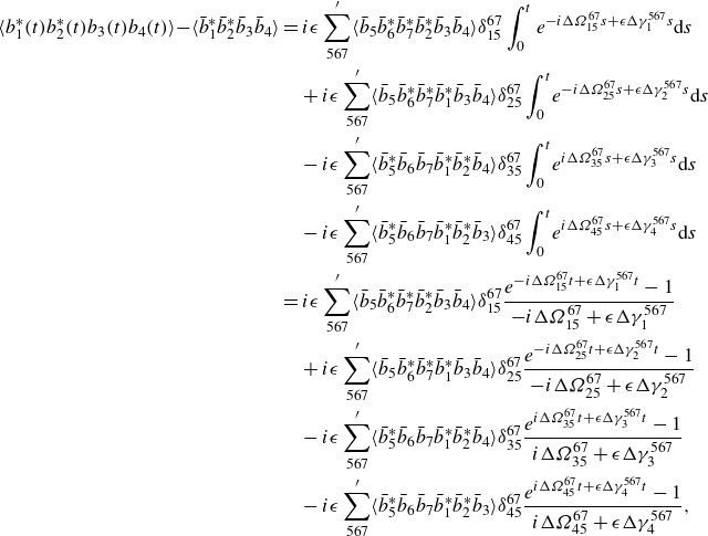 \begin{align} \langle b_1^*(t)b_2^*(t)b_3(t)b_4(t)\rangle\! -\!\langle \bar {b}_1^*\bar {b}_2^*\bar {b}_3\bar {b}_4\rangle &=i\epsilon \sum ^{\prime }_{567}\langle \bar {b}_5\bar {b}_6^*\bar {b}_7^*\bar {b}_2^*\bar {b}_3\bar {b}_4\rangle \delta _{15}^{67}\int _0^{t}e^{-i\Delta \Omega _{15}^{67}s+\epsilon \Delta \gamma _{1}^{567}s}\textrm {d} s\nonumber \\ &\quad +i\epsilon \sum ^{\prime }_{567}\langle \bar {b}_5\bar {b}_6^*\bar {b}_7^*\bar {b}_1^*\bar {b}_3\bar {b}_4\rangle \delta _{25}^{67}\int _0^{t}\!e^{-i\Delta \Omega _{25}^{67}s+\epsilon \Delta \gamma _{2}^{567}s}\textrm {d} s\nonumber \\ &\quad -i\epsilon \sum ^{\prime }_{567}\langle \bar {b}_5^*\bar {b}_6\bar {b}_7\bar {b}_1^*\bar {b}_2^*\bar {b}_4\rangle \delta _{35}^{67}\int _0^{t}\!e^{i\Delta \Omega _{35}^{67}s+\epsilon \Delta \gamma _{3}^{567}s}\textrm {d} s\nonumber \\ &\quad -i\epsilon \sum ^{\prime }_{567}\langle \bar {b}_5^*\bar {b}_6\bar {b}_7\bar {b}_1^*\bar {b}_2^*\bar {b}_3\rangle \delta _{45}^{67}\int _0^{t}\!e^{i\Delta \Omega _{45}^{67}s+\epsilon \Delta \gamma _{4}^{567}s}\textrm {d} s\nonumber \\ &=i\epsilon \sum ^{\prime }_{567}\langle \bar {b}_5\bar {b}_6^*\bar {b}_7^*\bar {b}_2^*\bar {b}_3\bar {b}_4\rangle \delta _{15}^{67}\frac {e^{-i\Delta \Omega _{15}^{67}t+\epsilon \Delta \gamma _{1}^{567}t}-1}{-i\Delta \Omega _{15}^{67}+\epsilon \Delta \gamma _{1}^{567}}\nonumber \\ &\quad +i\epsilon \sum ^{\prime }_{567}\langle \bar {b}_5\bar {b}_6^*\bar {b}_7^*\bar {b}_1^*\bar {b}_3\bar {b}_4\rangle \delta _{25}^{67}\frac {e^{-i\Delta \Omega _{25}^{67}t+\epsilon \Delta \gamma _{2}^{567}t}-1}{-i\Delta \Omega _{25}^{67}+\epsilon \Delta \gamma _{2}^{567}}\nonumber \\ &\quad -i\epsilon \sum ^{\prime }_{567}\langle \bar {b}_5^*\bar {b}_6\bar {b}_7\bar {b}_1^*\bar {b}_2^*\bar {b}_4\rangle \delta _{35}^{67}\frac {e^{i\Delta \Omega _{35}^{67}t+\epsilon \Delta \gamma _{3}^{567}t}-1}{i\Delta \Omega _{35}^{67}+\epsilon \Delta \gamma _{3}^{567}}\nonumber \\ &\quad -i\epsilon \sum ^{\prime }_{567}\langle \bar {b}_5^*\bar {b}_6\bar {b}_7\bar {b}_1^*\bar {b}_2^*\bar {b}_3\rangle \delta _{45}^{67}\frac {e^{i\Delta \Omega _{45}^{67}t+\epsilon \Delta \gamma _{4}^{567}t}-1}{i\Delta \Omega _{45}^{67}+\epsilon \Delta \gamma _{4}^{567}}, \end{align}
where we assumed that the six points correlator does not evolve in time and therefore all terms in the six points correlators are equal to their value at initial time
 $\bar {b}_{\mathbf {k}}\equiv b_{\mathbf {k}}(0)$
. This corresponds to the condition of closure
$\bar {b}_{\mathbf {k}}\equiv b_{\mathbf {k}}(0)$
. This corresponds to the condition of closure
 \begin{align} \frac {\textrm {d} \langle b_j^*b_6^*b_7^*b_3b_4b_5\rangle }{\textrm {d} t}=\mathcal {O}(\epsilon ),\quad j=1,2\qquad \frac {\textrm {d} \langle b_1^*b_2^*b_5^*b_ib_6b_7\rangle }{\textrm {d} t}=\mathcal {O}(\epsilon ),\quad i=3,4. \end{align}
We now insert (D4) into (D2) and we obtain
 \begin{align} \frac {\textrm {d} |b_1|^2}{\textrm {d} t}=&\; 2\epsilon ^2\sum ^{\prime }_{\substack {234\\567}}\mathfrak {Im}\Bigg \{\langle \bar {b}_1^*\bar {b}_2^*\bar {b}_3\bar {b}_4\rangle e^{i\Delta \Omega _{12}^{34}t+\epsilon \Delta \gamma _{1}^{234}t}\nonumber \\ &+i\langle \bar {b}_5\bar {b}_6^*\bar {b}_7^*\bar {b}_2^*\bar {b}_3\bar {b}_4\rangle \delta _{15}^{67}\frac {e^{-i\Delta \Omega _{15}^{67}t+\epsilon \Delta \gamma _{1}^{567}t}-1}{-i\Delta \Omega _{15}^{67}+\epsilon \Delta \gamma _{1}^{567}}e^{i\Delta \Omega _{12}^{34}t+\epsilon \Delta \gamma _{1}^{234}t}\nonumber \\ &+i\langle \bar {b}_5\bar {b}_6^*\bar {b}_7^*\bar {b}_1^*\bar {b}_3\bar {b}_4\rangle \delta _{25}^{67}\frac {e^{-i\Delta \Omega _{25}^{67}t+\epsilon \Delta \gamma _{2}^{567}t}-1}{-i\Delta \Omega _{25}^{67}+\epsilon \Delta \gamma _{2}^{567}}e^{i\Delta \Omega _{12}^{34}t+\epsilon \Delta \gamma _{1}^{234}t}\nonumber \\ &-i\langle \bar {b}_5^*\bar {b}_6\bar {b}_7\bar {b}_1^*\bar {b}_2^*\bar {b}_4\rangle \delta _{35}^{67}\frac {e^{i\Delta \Omega _{35}^{67}t+\epsilon \Delta \gamma _{3}^{567}t}-1}{i\Delta \Omega _{35}^{67}+\epsilon \Delta \gamma _{3}^{567}}e^{i\Delta \Omega _{12}^{34}t+\epsilon \Delta \gamma _{1}^{234}t}\nonumber \\ &-i\langle \bar {b}_5^*\bar {b}_6\bar {b}_7\bar {b}_1^*\bar {b}_2^*\bar {b}_3\rangle \delta _{45}^{67}\frac {e^{i\Delta \Omega _{45}^{67}t+\epsilon \Delta \gamma _{4}^{567}t}-1}{i\Delta \Omega _{45}^{67}+\epsilon \Delta \gamma _{4}^{567}} e^{i\Delta \Omega _{12}^{34}t+\epsilon \Delta \gamma _{1}^{234}t}\Bigg \}\delta _{12}^{34}. \end{align}
The first term in the curly brackets can be evaluated by using Wick’s decomposition
 \begin{align} \langle b_1^*b_2^*b_3b_4\rangle =|b_3|^2|b_4|^2(\delta _3^1\delta _4^2+\delta _3^2\delta _4^1), \end{align}
so that
 \begin{align} \langle \bar {b}_1^*\bar {b}_2^*\bar {b}_3\bar {b}_4\rangle =|\bar {b}_3|^2|\bar {b}_4|^2(\delta _3^1\delta _4^2+\delta _3^2\delta _4^1)e^{i\Delta \Omega _{12}^{34}t+\epsilon \Delta \gamma _{1}^{234}t}=|\bar {b}_1|^2|\bar {b}_2|^2 e^{-2\epsilon \gamma _2 t}, \end{align}
which we note is a pure real quantity and hence, it will not give contribution to (D2). The other terms in the curly brackets can be evaluated again by using Wick’s decomposition: for instance, for the second term in (D6) we can use
 \begin{align} \langle b_3b_4b_5b_2^*b_6^*b_7^*\rangle &=|b_2|^2|b_6|^2|b_7|^2\left (\delta _{3}^{2}\delta _{4}^{6}\delta _{5}^{7}+\delta _{3}^{6}\delta _{4}^{7}\delta _{5}^{2}+\delta _{3}^{7}\delta _{4}^{2}\delta _{5}^{6}+\delta _{3}^{2}\delta _{4}^{7}\delta _{5}^{6}+\delta _{3}^{7}\delta _{4}^{6}\delta _{5}^{2}\right. \nonumber\\&\quad \left. +\delta _{3}^{6}\delta _{4}^{2}\delta _{5}^{7}\right ), \end{align}
and the non-trivial terms are those proportional to
 $\delta _{3}^{6}\delta _{4}^{7}\delta _{5}^{2}$
and
$\delta _{3}^{6}\delta _{4}^{7}\delta _{5}^{2}$
and
 $\delta _{3}^{7}\delta _{4}^{6}\delta _{5}^{2}$
. Evaluating both terms leads to
$\delta _{3}^{7}\delta _{4}^{6}\delta _{5}^{2}$
. Evaluating both terms leads to
 \begin{align} 2i|\bar {b}_2|^2|\bar {b}_3|^2|\bar {b}_4|^2\frac {e^{-i\Delta \Omega _{12}^{34}t+\epsilon \Delta \gamma _{1}^{234}t}-1}{-i\Delta \Omega _{12}^{34}+\epsilon \Delta \gamma _{1}^{234}} e^{i\Delta \Omega _{12}^{34}t+\epsilon \Delta \gamma _{1}^{234}t}\delta _{12}^{34}. \end{align}
Rationalizing the denominator and removing the term proportional to
 $\epsilon$
, which gives an overall
$\epsilon$
, which gives an overall
 $\epsilon ^3$
contribution, leads to
$\epsilon ^3$
contribution, leads to
 \begin{align} -2|\bar {b}_2|^2|\bar {b}_3|^2|\bar {b}_4|^2\frac {\Delta \Omega _{12}^{34}\left (e^{-i\Delta \Omega _{12}^{34}t+\epsilon \Delta \gamma _{1}^{234}t}-1\right )}{\left (\Delta \Omega _{12}^{34}\right )^2+\left (\epsilon \Delta \gamma _{1}^{234}\right )^2} e^{i\Delta \Omega _{12}^{34}t+\epsilon \Delta \gamma _{1}^{234}t}\delta _{12}^{34}. \end{align}
Carrying out the multiplication gives
 \begin{align} -2|\bar {b}_2|^2|\bar {b}_3|^2|\bar {b}_4|^2\frac {\Delta \Omega _{12}^{34}\left (e^{2\epsilon \Delta \gamma _{1}^{234}t}-e^{\epsilon \Delta \gamma _1^{234}t}\cos \left (\!\Delta \Omega _{12}^{34}t\right )-i\sin \left (\!\Delta \Omega _{12}^{34}t\right )e^{\epsilon \Delta \gamma _{1}^{234}t}\right )}{\left (\Delta \Omega _{12}^{34}\right )^2+\left (\epsilon \Delta \gamma _{1}^{234}\right )^2}\delta _{12}^{34}. \end{align}
According to (D2) we only need to consider the imaginary part so we have
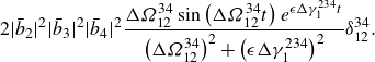 \begin{align} 2|\bar {b}_2|^2|\bar {b}_3|^2|\bar {b}_4|^2\frac {\Delta \Omega _{12}^{34}\sin \left (\Delta \Omega _{12}^{34}t\right )e^{\epsilon \Delta \gamma _{1}^{234}t}}{\left (\Delta \Omega _{12}^{34}\right )^2+\left (\epsilon \Delta \gamma _{1}^{234}\right )^2}\delta _{12}^{34}. \end{align}
The calculation for the other terms can be done in analogous way and, after inserting all terms into (D6), we recover (3.31) for
 $m=1$
.
$m=1$
.


 Open access