Asymmetric instability of flow-induced vibration for elastically mounted cube at moderate Reynolds numbers

Abstract

The asymmetric instability in two streamwise orthogonal planes for three-dimensional flow-induced vibration (FIV) of an elastically mounted cube at a moderate Reynolds number of 300 is numerically investigated in this paper. The full-order computational fluid dynamics method, data-driven stability analysis via the eigensystem realization algorithm and the selective frequency damping method and total dynamic mode decomposition (TDMD) are applied here to explore this problem. Due to the unsteady non-axisymmetric wakefield formed for flow passing a stationary cube, the FIV response was found to exhibit separate structural stability and oscillations (including lock-in and galloping behaviour) in the two different streamwise orthogonal planes while the body is released. The initial kinetic energy accompanying the release of the cube could destabilize the above-mentioned structural stability. The observed FIV asymmetric instability is verified by the root trajectory of the structural mode obtained via data-driven stability analysis. The stability of the structural modes dominates regardless of whether the structural response oscillates significantly in various (reduced) velocity ranges. Further TDMD analysis on the wake structure, accompanied by the time–frequency spectrum of time-history structural displacements, suggested that the present FIV unit with galloping behaviour is dominated by the combination of the shifted base-flow mode, structure modes and several harmonics of the wake mode.

1. Introduction

Flow-induced vibration (FIV) is one kind of fluid–solid coupling behaviour quite common in nature as well as in industrial environments, and it also widely exists in the fields of marine science, aerospace, energy and medicine. The works of Sarpkaya (1979), Parkinson (1989), Williamson & Govardhan (2004) and Ma et al. (2022) have comprehensively reviewed the FIV phenomenon. The generation of FIV is caused by the interaction between the fluid and the elastically supported and/or flexible structure. From the mechanism perspective, FIV patterns are classified as lock-in (resonance and flutter), galloping, buffeting, surge, etc. (Modi & Munshi 1998; Waals, Phadke & Bultema 2007). Aside from having potential utility when applied to energy extractors, FIV may cause fatigue/fracture to these mechanical structures and therefore cause threat to life.

Geometric shapes have a decisive influence on the response of FIV, and past research on FIV has explored a multitude of shapes, such as circular cylinders (Navrose & Sanjay 2016; Huera-Huarte 2020; Domínguez, Piedra & Ramos 2021), square cylinders (Zhao, Cheng & Zhou 2013; Li et al. 2019), trapezoids (Wang et al. 2021; Zhu et al. 2021), spheres (Jauvtis, Govardhan & Williamson 2001; Govardhan & Williamson 2005; Rajamuni, Thompson & Hourigan 2018, 2020; Chizfahm, Joshi & Jaiman 2021), airfoils (Besem et al. 2015; Derakhshandeh et al. 2016), etc. These studies have provided insights into the vibrational characteristics of the various shapes. However, there is much less attention on the FIV of cubes. To our knowledge, the only works on the FIV study of a cube are the experimental measurements carried out by Zhao et al. (2019). Zhao et al. experimentally measured the vibration response of the elastically mounted cube at different angles of attack, with the accompanying Reynolds number $Re$ varying from 2840 to 36 595. At all three angles of attack (specifically, 0$^{\circ }$, 20$^{\circ }$ and 45$^{\circ }$), the systems of concern all eventually exhibited galloping behaviour as the incoming velocity (reduced velocity) increased. The detailed division of the synchronization regions depends on the locking relationship between the various dynamics coefficients. However, the work of Zhao et al. (2019) only tabulated the response characteristics for different configurations from the characterization of the measured data. There has been no relevant study to investigate the mechanism of the FIV of the cube from the modal point of view. In addition, there is an absence of investigations that deal with the cube's FIV in the case of low to moderate Reynolds numbers. As we have discovered in this study, the system of flow past a cube has special wake dynamic features at Reynolds numbers in the low to moderate range.

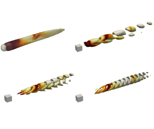
Following the previous works of Khan, Sharma & Agrawal (2019), Saha (2004) and Klotz et al. (2014), we calculate three typical wake structures for flow past a cube and present these in figure 1. The correlated wake structures evolve from steady axisymmetric to steady non-axisymmetric and then to unsteady non-axisymmetric with increasing Reynolds number. In detail, the wake is stable and symmetrical at $Re$ less than 200, as shown in figure 1(a). In this $Re$ interval, as $Re$ increases the drag coefficient decreases while the recirculation length increases. This symmetric structure will collapse as $Re$ rises to approximately 200–215. With respect to range of $215 < Re < 250$, the symmetry of one streamwise orthogonal plane is maintained while the asymmetry of the other plane is triggered (cf. figure 1b) due to the lack of viscous force balancing the centrifugal force separating the bubbles, there is a transfer of fluid from one vortex to another (Saha 2004). When the Reynolds number increases to a threshold (approximately equal to 270), Hopf bifurcation occurs and causes the wake structure to become unsteady. In this case, the flow structure forms symmetric behaviour in one plane and asymmetric behaviour in the other plane, as exhibited in figure 1(c). As $Re$ is further increased to around 340, the symmetric structure on the streamwise orthogonal planes completely disappears and the system becomes unsteady and non-axisymmetric in all directions. Considering the specific characteristics (i.e. symmetric on one plane, asymmetric on the other and overall vortex shedding) of flow past a stationary cube at $Re= $ 300, we have chosen this configuration here as the basis for the study of the cube's FIV in this paper.

Figure 1. Instantaneous streamline visualization (via line integral convolution vector methodology) at two streamwise orthogonal planes for flow passing a cube at Reynolds numbers of (a) 150, (b) 250 and (c) 300. Panels show (a) $Re = 150$: steady axisymmetric, (b) $Re = 250$: steady non-axisymmetric, (c) $Re = 300$: unsteady non-axisymmetric.

To study the mechanism underlying FIV, previous studies have tried to explore, from a modal perspective, the flow–structure coupling behaviour using data-driven stability analysis. The data-driven methodologies applied in FIV research include linear stability analysis (LSA) (Zhang et al. 2015; Yao & Jaiman 2017), global stability analysis (Navrose & Sanjay 2016), machine learning (Amir & Rajeev 2022), etc. Zhang et al. (2015) carried out a LSA of vortex-induced vibration of a circular cylinder using the reduced-order model based on the autoregressive with exogenous input (ARX) identification method. The modes dominating the FIV system involve the structure mode (SM) and wake mode (WM), whose internal coupling will have a significant impact on the system response. Besides the ARX method, Yao & Jaiman (2017) and Cheng et al. (2022c) applied the eigensystem realization algorithm (ERA) identification technology to conduct linear stability analysis for the two-dimensional (2-D) FIV system. The above stability method sought to explain the various behaviours/phenomena in FIV fields through modal interactions, transformation and competition. The present work will apply the ERA identification method to the LSA of the configuration of interest, and the detailed methodology will be introduced in the next section.

This work will explore the detailed characterization of the cube's FIV response and the mechanisms underlying the complex dynamics based on: (i) full-order results obtained using computational fluid dynamics (CFD) methods; (ii) data-driven modal analyses based on the ERA and selective frequency damping method; and (iii) analysis via the total dynamic modal decomposition of the wake dynamics.

The paper is structured as follows: § 2 details the numerical and analytical methods listed above. The accuracy of the implemented models used herein is validated carefully and systematically in § 3. In § 4, the asymmetric structural instability in two transverse directions for the FIV of the cube is analysed. The detailed response features and wake dynamics are also explored. Finally, in § 5, the key results of this study are summarized.

2. Numerical methodology

2.1. Computational fluid dynamics

For the configuration of interest in this work, which is an elastically mounted cube submerged in a three-dimensional (3-D) uniform flow, a full-order model (FOM) CFD method is first applied to calculate the FIV response. In more detail, the governing equations of the flow dynamics are the unsteady incompressible Navier–Stokes (NS) equations, while the boundary changes induced by the cube's motion are resolved based on an arbitrary Lagrangian–Eulerian (ALE) scheme. The NS equations in the ALE scheme are expressed as

(2.1)\begin{equation} \frac{\partial u_i}{\partial x_i}=0, \end{equation}

and

(2.2)\begin{equation} \frac{\partial u_i}{\partial t}+\left( u_j-\hat{u}_j \right) \frac{\partial u_i}{\partial x_j}={-}\frac{1}{\rho}\frac{\partial p}{\partial x_i}+\nu \frac{\partial ^2u_i}{\partial x_{i}\partial x_{j}}, \end{equation}

where $u_i$ is the velocity component in the $x_i$-direction of fluid flow, $\hat {u}_i$ is the component of mesh movement velocity in the $x_i$-direction, $( x_1,x_2,x_3 )= ( x,y,z )$ are the Cartesian coordinates, $p$ is the pressure and $t$ is the time; $\rho$ and $\nu$ are the density and kinematic viscosity of the fluid, respectively.

The dimensionless structural equation controlling the transverse vibration of the cube is given by the following:

(2.3)\begin{equation} \ddot{h_i}+4{\rm \pi} F_s \zeta \dot{h_i}+\left( 2{\rm \pi} F_s \right) ^2h_i={C_i}/2{m^*} , \end{equation}

where $F_s = f_n D/U_{0} \equiv U_r^{-1}$ is the reduced natural frequency ($D$ is the side length of the cube, $f_n$ is the structural natural frequency, $U_0$ is the incident flow velocity and $U_r$ is the reduced velocity); $m^*=\rho _s/\rho$ is the mass ratio ($\rho _s$ is the body density and $\rho$ is the fluid density); $h_i$ is the non-dimensional transverse displacement in the $x_i$-direction normalized by $D$; $C^i$ is the lift coefficient in the $x_i$-direction; and, $\zeta$ is the structural damping coefficient.

OpenFOAM (2017), an open-source software for CFD developed by the OpenFOAM Foundation, is applied for the flow field simulations herein. The NS equations are discretized by the finite volume method. The transient terms are discretized using the second-order implicit Eulerian scheme, and the advection, pressure gradient and diffusion terms are discretized using the second-order Gaussian integration scheme. The large time-step transient PIMPLE (merged PISO-SIMPLE) algorithm, which combines the semi-implicit method for pressure-linked equations (SIMPLE) and the pressure implicit with the splitting of operators (PISO) algorithm, is used to solve the continuity and momentum transport equations together in a segregated manner. All of these algorithms are iterative solvers, but PISO and PIMPLE are used for transient problems, whereas SIMPLE is used herein for steady-state problems. The pressure–velocity coupling provided by the PIMPLE algorithm results in better stability and higher accuracy when large time steps are applied (Penttinen, Yasari & Nilsson 2011). In this case, an adaptive time-step technique is used herein to ensure that the maximum Courant–Friedrichs–Lewy (CFL) number ${\rm CFL}_{max}$ is limited to 5 (${\rm CFL}_{max} \equiv {\|\vec u \|\Delta t}/{\Delta x_{min}}$, where $\|\vec u\|$ is the magnitude of the fluid velocity $\vec u$, $\Delta t$ is the time step and $\Delta x_{min}$ is the size of the smallest grid cell in the computational domain). Additionally, the iteration number for SIMPLE (steady-state) treatment and pressure–momentum coupling inside PIMPLE are fixed at 50 and 2, respectively, for each time step in the present work. An explicit second-order symplectic method (Dullweber, Leimkuhler & McLachlan 1997) is applied to integrate the structural equations of motion. The weakly coupled approach (Wang et al. 2019) is applied to solve the fluid–structure interaction that links the fluid flow equations ((2.1) and (2.2)) with the structural equation of motion (2.3).

2.2. Data-driven modal analysis

This section provides a brief description of the reduced-order model (ROM) for the FIV system and the associated stability analysis. More detailed information is provided in our previous works (Cheng et al. 2022c, 2023b). Several key steps in constructing the final coupled ROM (represented as a state-space model) for the FIV system being considered are depicted in figure 2. The final coupled fluid–solid model contains two parts: the linear fluid model and the structural model. The linear fluid model is herein represented by the state-space model obtained by ERA (described in detail later), with inputs $h_i \equiv y/D$ or $z/D$ and outputs $C_i$ ($i= 2$ and 3 denote $y$- and $z$-directions, respectively). The structural model is derived from the motion control equations and is also expressed as a state-space model with input $C_i$ and output $h_i$. Finally, the above two state-space models will be coupled together as described above. The detailed steps are described below:

Figure 2. Flow diagram summarizing the five key steps in the workflow to obtain the ROM/ERA for a FIV system involving the coupling of a fluid dynamics ROM (with input $h_i$ and output $C_i$) to a structural dynamics model (with input $C_i$ and output $h_i$).

The first step of the workflow is to apply FOM/CFD calculation to obtain the equilibrium base flow passing the stationary structure. The steps to obtain the equilibrium base flow for the 2-D case can be found in our past work (Cheng et al. 2022c, 2023b), and the selective frequency damping (SFD) (introduced later) will be applied for obtaining the equilibrium base flow of the 3-D situation in the present work. The equilibrium base flow surrounding the structure could be viewed as a dynamical system with displacement inputs and lift outputs. More specifically, the inputs are the normalized transverse displacements $u_r \equiv h_i$ and the outputs are the lift coefficients $o_r \equiv C_i$ . We then model the fluid dynamics system using a discrete-time state-space model as follows:

(2.4)$$\begin{gather} x_r\left( k+1 \right) =\tilde{A}_r x_r\left( k \right) +\tilde{B}_r u_r\left( k \right), \end{gather}$$

(2.5)$$\begin{gather}o_r\left( k \right) =\tilde{C}_rx_r\left( k \right) +\tilde{D}_ru_r\left( k \right) , \end{gather}$$

where $x_r(k)$ is the $N_x$-dimensional state vector, $u_r(k)$ is the $N_u$-dimensional input vector and $o_r(k)$ is the $N_y$-dimensional output vector obtained at discrete-time step $k$. Here, it is noted that $t_k \equiv k\Delta t$ is the time associated with the $k$th discrete-time step, where $\Delta t$ is the time-step size. Immediately following the second step of the workflow, the dynamical system described above is given a discrete-time Kronecker delta function input $u_r^\delta$ (or impulse function) with amplitude $A_\delta$

(2.6)\begin{equation} u_r^\delta\left( k \right) \equiv u_r^\delta(t_k) = A_\delta\begin{cases} 1, & k=0;\\ 0, & k=1,2,3, \ldots . \\ \end{cases} \end{equation}

This impulse will lead to the impulse response $o_r^\delta (k) \equiv o_r^\delta (k\Delta t)$ of the dynamical system

(2.7)\begin{equation} o_r^\delta(k) \equiv o_r^\delta(k\Delta t) = \begin{cases}{\tilde D}_r, & k = 0;\\ {\tilde C}_r{\tilde A}_r^{k-1}{\tilde B}_r, & k = 1,2,3,\ldots , \end{cases} \end{equation}

in which the impulse response is the time series of the corresponding coefficients $C_i$ of the stationary body after it has been transversely displaced by the impulsive inputs (cf. (2.6)) in the $x_i$-direction).

The third step of the workflow will be to construct a low-dimensional linear input–output state-space model of the dynamic system based on the ERA. This work is achieved by stacking the time series of the impulse response $o_r^\delta$ (obtained in step 2) to construct the $(r\times s)$ Hankel matrix

(2.8)\begin{equation} \boldsymbol{\mathsf{Hc}} =\left[ \begin{matrix} o_r^\delta(1) & o_r^\delta(2) & \cdots & o_r^\delta(s)\\ o_r^\delta(2) & o_r^\delta(3) & \cdots & o_r^\delta(s+1)\\ \vdots & \vdots & \ddots & \vdots\\ o_r^\delta(r) & o_r^\delta(r+1) & \cdots & o_r^\delta(s+r-1)\\ \end{matrix} \right] . \end{equation}

The corresponding shifted Hankel matrices of the same size are as follows:

(2.9)\begin{equation} \widetilde{\boldsymbol{\mathsf{Hc}}} =\left[ \begin{matrix} o_r^\delta(2) & o_r^\delta(3) & \cdots & o_r^\delta(s+1)\\ o_r^\delta(3) & o_r^\delta(4) & \cdots & o_r^\delta(s+2)\\ \vdots & \vdots & \ddots & \vdots\\ o_r^\delta(r+1) & o_r^\delta(r+2) & \cdots & o_r^\delta(s+r)\\ \end{matrix} \right] . \end{equation}

Next, a singular value decomposition of the Hankel matrix $\boldsymbol{\mathsf{Hc}}$ yields (the superscript ${\rm T}$ denotes matrix transpose)

(2.10)\begin{equation} \boldsymbol{\mathsf{Hc}} = U\varSigma V^{\rm T}= \left[ U_1\,\,U_2 \right] \left[ \begin{matrix} \varSigma _1 & 0\\ 0 & \varSigma _2\\ \end{matrix} \right] \left[ \begin{matrix} V_{1}^{T}\\ V_{2}^{T}\\ \end{matrix} \right], \end{equation}

where $U$ is a $r\times r$ orthonormal matrix with columns containing the left singular vectors, $\varSigma$ is a $r\times s$ rectangular ‘diagonal’ matrix with diagonal entries containing the non-negative singular values in non-decreasing order, and $V$ is a $s\times s$ orthonormal matrix with columns containing the right singular vectors. Here, we select the rows and columns of the spectral decomposition corresponding to the dominating modes only, so the negligible modes represented by the tiny singular values in the diagonal matrix $\varSigma _2$ are omitted. Consequently, only the first $l$ singular values in $\varSigma _1$ are retained.

The Hankel matrix representing the relevant physical modes is estimated using the truncated singular value decomposition $\hat{\boldsymbol{\mathsf{H}}} = U_1\varSigma _1V_{1}^{T} = \sum _{k=1}^{l}\sigma _{kk}{\bar u}_k{\bar v}_k^{\rm T}$ where the positive singular values $\sigma _{kk}$ are the $(k,k)$th entries of the diagonal matrix $\varSigma _1$ ordered by their non-decreasing value, ${\bar u}_k$ is the $k$th column of $U$ (left singular vector) and ${\bar v}_k$ is the $k$th column of $V$ (right singular vector). This reduced decomposition of $\boldsymbol{\mathsf{Hc}}$ provides a rank-$l$ approximation of the $(r\times s)$ Hankel matrix $\hat{\boldsymbol{\mathsf{H}}}$. More specifically, the Hankel matrix $\hat{\boldsymbol{\mathsf{H}}}$ provides a low-rank approximation for the dynamical system and, as such, represents the significant temporal patterns in the time sequence impulse response data. Finally, the system matrices $(\tilde A_r, \tilde B_r, \tilde C_r, \tilde D_r)$ for the discrete-time state-space model (ROM) are estimated in accordance to

(2.11)$$\begin{gather} \bar{A}_r = \varSigma _{1}^{{-}1/2}U_{1}^{T} \widetilde{\boldsymbol{\mathsf{Hc}}} V_1\varSigma _{1}^{{-}1/2}; \end{gather}$$

(2.12)$$\begin{gather}\bar{B}_r = \varSigma _{1}^{1/2}V_{1}^{T}E_m ; \end{gather}$$

(2.13)$$\begin{gather}\bar{C}_r = E_{t}U_1\varSigma _{1}^{1/2}; \end{gather}$$

(2.14)$$\begin{gather}\bar{D}_r = o_r^\delta(0), \end{gather}$$

where

(2.15a,b)\begin{equation} E_m = \begin{bmatrix} I_q & 0 \end{bmatrix}^{\rm T} \quad {\rm and} \quad E_t = \begin{bmatrix} I_p & 0 , \end{bmatrix} \end{equation}

are used to extract the first $q$ columns and first $p$ rows in order to create $\bar B_r$ and $\bar C_r$, respectively. Here, $I_n$ is the identity matrix of order $n$. In the current investigation, the dimensionless transverse displacement ($h_i$) and lift coefficient ($C_i$), respectively, are the input ($u_r$) and output ($o_r$), so $p = q= 1$.

Finally, the system matrices for the discrete-time state-space model, $(\tilde A_r, \tilde B_r, \tilde C_r, \tilde D_r)$, are transformed into the system matrices for the corresponding continuous-time state-space model using the relationships $A_r= \Delta t^{-1} \ln (\bar {A}_r)$, $B_r=A_r[ \bar {A}_r-I ] ^{-1}\bar {B}_r$, $C_r=\bar {C}_r$ and $D_r=\bar {D}_r$, where $I$ is an identity matrix of the same size as $\bar A_r$ (Shieh, Wang & Yates 1980). The fluid flow system's continuous-time state-space model then takes the following form:

(2.16)\begin{equation} \left. \begin{aligned} \dot{x}_r\left( t \right) & =A_rx_r\left( t \right) +B_ru_r\left( t \right) ,\\ o_r\left( t \right) & =C_rx_r\left( t \right) +D_ru_r\left( t \right) . \end{aligned} \right\} \end{equation}

The dimensionless structural equation of motion provided by

(2.17)\begin{equation} \ddot{h_i}+4{\rm \pi} F_s \zeta \dot{h_i}+\left( 2{\rm \pi} F_s \right) ^2h_i={a_sC_i}/{m^*}, \end{equation}

is transformed into a representation of continuous-time state-space in the fourth step of the workflow. With input $C_i$ and output $h_i$, (2.17) may be converted into a continuous-time state-space form as follows:

(2.18)\begin{equation} \left. \begin{aligned} \dot{x}_s\left( t \right) & =A_sx_s\left( t \right) +qB_s o_r\left( t \right) ,\\ h_i\left( t \right) & =C_sx_s\left( t \right) +qD_s o_r\left( t \right) , \end{aligned} \right\} \end{equation}

with the structural system's state vector $x_s \equiv (h_i,\dot {h_i} )^\textrm {T}$, $q\equiv {a_s}/{m^*}$ and

(2.19a–d)\begin{equation} A_s=\left[ \begin{matrix} 0 & 1\\ -\left( 2{\rm \pi} F_s \right) ^2 & -4{\rm \pi} F_s c\\ \end{matrix} \right], \quad B_s=\left[ \begin{matrix} 0\\ 1\\ \end{matrix} \right], \quad C_s=\left[ 1\ 0 \right], \quad D_s=\left[ 0 \right]. \end{equation}

Here, $F_s = f_n D/U_{0} \equiv U_r^{-1}$ is the reduced natural frequency. Finally, a characteristic length scale $a_s$ (cf. (2.17)) is determined by the geometry of the body as

(2.20)\begin{equation} a_s=\frac{1}{A_b} \cdot \frac{D^{2}}{2}, \end{equation}

where $A_b$ and $D$ are the cross-sectional area and characteristic length of the bluff body, respectively, and $a_s$ is equal to 1/2 for the cube in this work.

In the fifth (and final) step of the workflow, the state-space model for the fluid flow system provided by (2.16) is coupled to the state-space model for the structural dynamics provided by (2.18) and (2.19a–d) to generate the linear and reduced-order coupled model for the FIV system. As a result, the linear and reduced model for the FIV system finally takes the following shape:

(2.21)$$\begin{gather} \dot{x}_{rs}\left( t \right) = \boldsymbol{A}_{rs} x_{rs}\left( t \right) \equiv \left[\begin{matrix}A_s+qB_sD_rC_s & q B_sC_r \\ B_rC_s & A_r\\ \end{matrix} \right] x_{rs}\left( t \right) , \end{gather}$$

(2.22)$$\begin{gather}h\left( t \right) = \left[ C_s\ 0 \right] x_{rs}\left( t \right), \end{gather}$$

where $x_{rs}\equiv ( x_s,x_r )^\textrm {T}$ is the state vector for the FIV system.

By examining the behaviour of the eigenvalues of the system matrix $\boldsymbol {A}_{rs}$ shown in (2.21), the FIV stability problem will be addressed. The system's two or three most dominant modes, which comprise both the SM and WM, are correlated to the two or three leading eigenvalues (which vary depending on the Reynolds number). Later in the study, we will detail our methods for identifying the SM/WM and how we interpret the physical processes connected to their behaviour. The system matrix $\boldsymbol {A}_{rs}$ complex eigenvalues determine the associated (eigen)mode's growth/decay rate and oscillatory properties. More specifically, the growth or decay rate of the mode is determined by the positivity or negativity of the real parts of the eigenvalues. Each eigenvalue's imaginary part corresponds to the accompanied mode's oscillatory (eigen)frequency. The (eigen)frequency of the mode is provided by the expression $\textrm {Im}(\lambda )/2{\rm \pi}$, where $\lambda$ is the (complex) eigenvalue and $\textrm {Im}( \cdot )$ stands for the imaginary part of a complex number.

While the flutter-induced lock-in and galloping behaviours are correlated with an unstable structure mode (i.e. when the real part of the eigenvalue associated with the SM is positive) and arise from the interaction between the SM and WM, the resonance lock-in results from the closeness in value of the frequency associated with the SM to those associated with the WMs. Furthermore, depending on whether there is a significant distinction between the root loci associated with the SM and WM, the modal behaviour of one FIV system is either coupled or uncoupled. It is required to establish which of the two coupled modes for one FIV system (which we refer to as WSMI and WSMII below) corresponds to the hidden structure-dominated mode for each value of the natural frequency ($F_s$). In fact, the hidden structure-dominated mode can start as WSMI at one value of $F_s$ and change to WSMII at a different value of $F_s$ (or vice versa), a process known as ‘mode veering’ (Gao et al. 2017). The hidden structure-dominated mode SM$_{c}$ is characterized in this study as the coupled mode with an eigenfrequency that is closest in value to the reduced natural frequency $F_s$. In this identification of the hidden structure-dominated mode, the reader is reminded by the subscript ‘c’ that this mode is correlated to the coupled status.

2.3. Selective frequency damping

For certain complex configurations where equilibrium base flow is difficult to obtain, the SFD method (Åkervik et al. 2006; Jordi, Cotter & Sherwin 2015; Casacuberta et al. 2018; Plante & Laurendeau 2018) can be used to obtain equilibrium base flow for carrying out further ERA identification. Specifically, the NS equations corresponding to (2.1) and (2.2) could be expressed in the following form:

(2.23)\begin{equation} \boldsymbol{\dot{q}}=\text{F}\left( \boldsymbol{q} \right). \end{equation}

The main strategy of SFD is to add a proportional feedback control to the right end of the equation

(2.24)\begin{equation} \boldsymbol{\dot{q}}={F}\left( \boldsymbol{q} \right) -\chi \left( \boldsymbol{q}-\boldsymbol{q}_{{s}} \right) . \end{equation}

It can be seen that, when $\boldsymbol {q}_{{s}}$ is a static solution of (2.24), $\boldsymbol {q}_{{s}}$ will also become a static solution of (2.23). However, there is a concern here in that $\boldsymbol {q}_{{s}}$ is not a variable that is known in advance. To address this, the SFD method changes the unknown $\boldsymbol {q}_{{s}}$ to a low-pass filtered solution $\boldsymbol {\bar {q}}$. At the same time, a new equation is added as the differential form of the low-pass temporal filter

(2.25) \begin{equation} \left\{\begin{aligned}& \boldsymbol{\dot{q}}=\text{F}\left( \boldsymbol{q} \right) -\chi \left( \boldsymbol{q}-\boldsymbol{\bar{q}} \right)\\ &\boldsymbol{\dot{\bar{q}}}=\omega _c\left( \boldsymbol{q}-\boldsymbol{\bar{q}} \right)\end{aligned}\right.. \end{equation}

A more detailed description of SFD can be found in other works (Richez, Leguille & Marquet 2016; Casacuberta et al. 2018; Plante & Laurendeau 2018). Thus, (2.1) and (2.2) will be rewritten as

(2.26)\begin{gather} \frac{\partial u_i}{\partial x_i}=0, \end{gather}

(2.27)\begin{gather} \frac{\partial u_i}{\partial t}+\left( u_j-\hat{u}_j \right) \frac{\partial u_i}{\partial x_j}={-}\frac{1}{\rho}\frac{\partial p}{\partial x_i}+\nu \frac{\partial ^2u_i}{\partial x_i\partial x_j}-\chi \left( u_i-\bar{u}_i \right), \end{gather}

and

(2.28)\begin{equation} \frac{\partial \bar{u}_i}{\partial t}=\omega _c\left( u_i-\bar{u}_i \right), \end{equation}

where $\chi$ is the filter gain and $\omega _c$ is the cutoff circular frequency. In the choice of parameters, $\chi$ must be positive and larger than the growth rate of the target unstable component, while $\omega _c$ must be lower than the eigenfrequency of the target unstable component.

2.4. Total dynamic mode decomposition

Dynamic mode decomposition (DMD) is a common data order reduction method. As a data-driven methodology, DMD, although not constrained by the physical model and governing equations, could be applied to directly extract the eigenmodes in the (time-varying) snapshot data provided by experimental measurements and/or numerical data, to accurately characterize the flow structure (Schmid 2010). The data snapshots could be presented in the form of matrices $\boldsymbol{\mathsf{X}}$ and $\boldsymbol{\mathsf{Y}}$

(2.29)$$\begin{gather} \boldsymbol{\mathsf{X}}=\left\{ \nu _1,\nu _2,\nu _3,\ldots ,\nu _{N-1} \right\} , \end{gather}$$

(2.30)$$\begin{gather}\boldsymbol{\mathsf{Y}}=\left\{ \nu _2,\nu _3,\nu _4,\ldots ,\nu _N \right\} , \end{gather}$$

where $\nu _i$ represents the flow field at the $i$th moment, and the snapshot sampling interval is $\delta t$. It is assumed that there is a linear mapping relationship $\boldsymbol{\mathsf{H}} \in \mathbb {R}^{M\times M}$ between the flow fields $\nu _i$ and $\nu _{i+1}$

(2.31)\begin{equation} \nu _{i+1} = \boldsymbol{\mathsf{H}} \nu _i , \end{equation}

and that the above relation is satisfied for the entire region and also over the entire time period. This process is a linear estimation process although the dynamical system itself is nonlinear to some degree. Thus the following relationship is satisfied between the sampled snapshot sequences:

(2.32)\begin{equation} \boldsymbol{\mathsf{Y}} = \boldsymbol{\mathsf{H}} \boldsymbol{\mathsf{X}} . \end{equation}

Thus, the system matrix $\boldsymbol{\mathsf{H}}$ is able to translate the time–space physical field along the time interval $\delta t$. The eigenvalues of $\boldsymbol{\mathsf{H}}$ characterize the time evolution of $\boldsymbol{\mathsf{Y}}$. However, $\boldsymbol{\mathsf{H}}$ is a indeed very high-dimensional matrix, so we would like to transform $\boldsymbol{\mathsf{H}}$ into a small low-dimensional equivalent matrix $\widetilde {\boldsymbol{\mathsf{Hc}}} \in \mathbb {R}^{r\times r}$. The DMD algorithm is to find the low-dimensional matrix $\widetilde {\boldsymbol{\mathsf{Hc}}}$ to replace the high-dimensional matrix $\boldsymbol{\mathsf{H}}$

(2.33)\begin{equation} \boldsymbol{\mathsf{H}}=\boldsymbol{U}_r \widetilde{\boldsymbol{\mathsf{Hc}}} \boldsymbol{U}_r^* , \end{equation}

where $\boldsymbol {U}_r$ can be obtained by (reduced) singular value decomposition (SVD) of $\boldsymbol{\mathsf{X}}$

(2.34)\begin{equation} \boldsymbol{\mathsf{X}}=\boldsymbol{U}_r \boldsymbol{\varSigma} \boldsymbol{V}_r^*, \end{equation}

where $\boldsymbol {\varSigma }$ is a diagonal matrix of dimension $r \times r$. $\boldsymbol {U}_r\in \mathbb {R}^{M\times r}, \boldsymbol {U}_r^*\boldsymbol {U}_r=\boldsymbol {I}, \boldsymbol {V}_r\in \mathbb {R}^{r\times N}, \boldsymbol {V}_r^*\boldsymbol {V}_r=\boldsymbol {I}$, where $\boldsymbol {I}$ is a unit matrix. Thus $\boldsymbol{\mathsf{H}}$ thereby could be approximated as

(2.35)\begin{equation} \boldsymbol{\mathsf{H}}\cong \widetilde{\boldsymbol{\mathsf{Hc}}}=\boldsymbol{U}_r^*\boldsymbol{\mathsf{Y}}\boldsymbol{V}_r \boldsymbol{\varSigma }^{{-}1}. \end{equation}

Since the matrix $\widetilde {\boldsymbol{\mathsf{Hc}}}$ is the low-dimensional approximation matrix of $\boldsymbol{\mathsf{H}}$, the eigenvalues of $\widetilde {\boldsymbol{\mathsf{Hc}}}$ are part of those of $\boldsymbol{\mathsf{H}}$, i.e. the Ritz eigenvalues. The eigenvalue of the $j$th mode is defined as $\mu _j$ and the corresponding eigenvector is $\boldsymbol {\omega }_j$. The corresponding DMD modality is defined as

(2.36)\begin{equation} \boldsymbol{\varPhi }_{j}=\boldsymbol{U}_r \boldsymbol{\omega }_{j}. \end{equation}

The stability characteristics of the corresponding modes can be determined by the Ritz eigenvalues (or modal growth rates). The preceding description of eigenmode identification using DMD is limited to the scenario with ‘perfect’ snapshot data. Indeed, in many cases when the data are imprecise and noisy, the underconstrained scenario is undesirable since solutions will definitely overfit the noise. To obtain noise-corrected snapshot data, the total DMD (TDMD) strategy is used, which projects the snapshot data onto an appropriate basis using projection $\mathbb {P}$ (the orthogonal projections are self-adjoint herein), the standard DMD algorithm can then be applied to the resulting corrected snapshot data to yield a de-biased characterization of the dynamics (Hemati et al. 2016, 2017). The TDMD procedure consists of the following workflow:

1. (i) correcting snapshot data via projection $\mathbb {P}$ ($=\boldsymbol {V}_r\boldsymbol {V}_r^*$): $\boldsymbol {\bar {\boldsymbol{\mathsf{X}}}}=\boldsymbol{\mathsf{X}}\mathbb {P}=\boldsymbol{\mathsf{X}}\boldsymbol {V}_r\boldsymbol {V}_r^*$;

2. (ii) conducting the SVD of ${\bar {\boldsymbol{\mathsf{X}}}}=\boldsymbol {\bar {U}\bar {\varSigma }\bar {V}}^*$;

3. (iii) constructing the de-biased proxy system $\boldsymbol {\bar {A}}:=\boldsymbol {\bar {U}}^*\boldsymbol{\mathsf{Y}}\boldsymbol {\bar {V}\bar {\varSigma }}^{-1}\in \mathbb {R}^{r\times r}$;

4. (iv) performing the eigenvalue decomposition $\boldsymbol {\bar {A}\omega }_j=\boldsymbol {\lambda }_{\boldsymbol {j}}\boldsymbol {\omega }_j$, the corresponding DMD modes are represented as:

   (2.37)\begin{equation} \boldsymbol{\varPhi }_j=\boldsymbol{\bar{U}\omega }_j. \end{equation}

The most significant feature of the DMD algorithm, despite its many variations (Hemati et al. 2017; Kiewat, Indinger & Tsubokura 2019), is that each DMD mode corresponds to a low-dimensional coherent spatio-temporal pattern in the data set and is associated with a distinctive complex frequency (or eigenvalue). The corresponding DMD (dynamical) mode's growth/decay and oscillatory properties are described by the Ritz eigenvalues. A convergent mode is represented by the Ritz eigenvalue falling within the unit circle with a growth rate less than zero; a divergent mode is represented by one falling outside the unit circle with a growth rate greater than zero; and a stable periodic mode is represented by one falling on the unit circle with a growth rate close to zero.

3. Computational domain and model validation

Figure 3 exhibits the configuration of one cube elastically supported by a linear spring unit and submerged in uniform inflow. With respect to the 3-D computational domain, the initial position of the cube centre is at the centreline of both transverse (or cross-stream) directions (i.e. $z=y= 0$), and situated at 8$D$ downstream from the inlet boundary in $x$-direction. The streamwise ($x$-) length and two cross-stream ($\kern0.09em y-, z$-) lengths of the computational domain are 43$D$, 16$D$ and 16$D$ leading to a blockage of 6.25 %, which is close to the those applied in the other FIV calculations of 3-D spheres and 2-D columns (Prasanth & Mittal 2008; Amir & Rajeev 2021, 2022). A Dirichlet boundary condition was prescribed for the incident flow velocity $\vec u = (U_x, 0, 0)$ on the inlet face annotated in blue in figure 3. A Neumann boundary condition is imposed on the velocity at the outflow (outlet) boundaries, i.e. the five face patches of the domain except the one coloured blue, to avoid potential blockage effects. The initial state of the cube's motion is assigned to be $y=0,\dot {y}=0,z=0,\dot {z}=0$. In light of the present focus on dynamical asymmetry of the FIV response and considering that the introduction above mentioned that wake dynamics for flow passing a stationary cube exhibits hairpin vortex shedding at $277 < Re < 350$, we chose $Re = 300$ for the incident flow environment. The hairpin vortex shedding means that the wake maintains stability in one cross-stream (or streamwise orthogonal) plane but becomes periodically time dependent with regular oscillations of the recirculation zone in another plane, as described in the Introduction section (Saha 2004; Klotz et al. 2014; Khan et al. 2019).

Figure 3. Three-dimensional computational domain applied in the present calculation for flow passing an elastically mounted cube submerged in uniform inflow.

The mesh dependency study is conducted via a 3-D simulation of uniform flow past an elastically mounted cube at $(Re, m^*, U_r) = (300, 15, 40)$. The corresponding FIV response for different mesh qualities is calculated and the associated results are summarized in table 1. The important parameters of the FIV response here include mean lift coefficients $C_{z, mean}$, root-mean-square (r.m.s.) drag coefficients $C_{x, rms}$ and maximum structural displacements $z_{max}$ in the $z$-direction. It can be seen that the relative differences of each parameter between mesh 1 to mesh 2 are considerable, but all decrease to a value smaller than 0.5 % as the mesh is refined to mesh 3 (fine) or mesh 4 (very fine). To follow up, we use mesh 3 to calculate the flow passing a stationary cube at $Re = 300$ and compare the drag coefficients between the present results and other accessible numerical works (Saha 2004; Khan et al. 2019). The results summarized in table 2 indicate high conformance between this study and other results. As a consequence, mesh 3 is adopted in the present work to achieve the best balance of calculation time and accuracy. Figure 4(a) displays the overview of the mesh domain used in the present study, with the expanded/close-up views of mesh in the immediate vicinity of the cube shown in figure 4(b).

Table 1. Maximum normalized structural displacements $z_{max}/D$ and aerodynamic coefficients (mean lift and root-mean-square drag coefficients $C_{z, mean}$ and $C_{x, rms}$) in the $z$-direction of flow past an elastically mounted cube at $Re= 300$ for different mesh conditions. Here, $\Delta x_{min}$ represents the size of the smallest grid cell.

Table 2. Drag coefficients for flow passing a stationary cube at $Re = 300$. The results are compared between Saha (2004), Khan et al. (2019) and the present work.

Figure 4. Mesh set-up (mesh 3) used in the present simulation. (a) Domain showing the overall mesh in one streamwise orthogonal $x\hbox{--}z$ plane (which is consistent with the mesh in the other streamwise orthogonal $x\hbox{--}y$ plane), and (b) domain showing the overall mesh in the transverse orthogonal $y\hbox{--}z$ plane, with an expanded view of the immediate vicinity of the cube walls.

To our knowledge, there are no available/accessible past works on the investigation of a cube's FIV response at moderate Reynolds numbers. To validate the accuracy of the implementation and prediction of present FOM/CFD, we first chose the square cylinder, whose cross-section is similar to the cube to some degree and was also proven to be able to induce galloping behaviours. The square cylinder is limited to moving in the transverse direction at $(Re, m^*) = (150, 10)$ with no structural damping. Furthermore, the FIV response of an elastically mounted 3-D sphere (also restricted to translate in the transverse direction) at $(Re, m^*, \zeta ) = (200, 10, 0.01)$ is calculated via the fluid-structure interaction (FSI) model implemented in the present work. The meshing construction strategy and refinement level of this validation case are comparable to those presented in figure 4. The reduced velocity $U_r$ is changed by modifying the spring stiffness for both validation cases. Present results of the square cylinder and sphere are compared with Li et al. (2019) and Rajamuni et al. (2018), respectively, in figures 5(a) and 5(b). The excellent agreement regarding normalized maximum structural displacements implies the correctness of the present fluid–structure coupling model, which is now demonstrated to be capable of providing good accuracy for FIV prediction in this work.

Figure 5. Comparison of the maximum normalized transverse structural displacement of flow passing an elastically mounted (a) square cylinder at $(Re, m^*, \zeta ) = (150, 10, 0)$ between the present work and Li et al. (2019), and (b) sphere at $(Re, m^*, \zeta ) = (200, 10, 0.01)$ between the present work and Rajamuni et al. (2018).

4. Discussion

4.1. Wake dynamics of stationary cube and description of the present FIV problem

Figure 6(a) shows the contour of the instantaneous velocity magnitude in the $x\hbox{--}y$ and $x\hbox{--}z$ orthogonal planes for flow past a cube at $Re = 300$. As introduced above, both numerical and experimental research have reported that the flow dynamics past a stationary cube at $Re = 300$ is classified as unsteady patterns with axisymmetric behaviour in one plane and non-axisymmetric behaviour in another plane (Klotz et al. 2014; Khan et al. 2019). This phenomenon is also observed by our present work, as displayed in figure 6(a,b) (which displays the 3-D vortex contour). It is clearly evident that a considerable fluctuation of the wake dynamics occurs in the $z$-direction, while in the $y$-direction, the vortex behaviours demonstrate a stable symmetry. This phenomenon is also verified by the dynamic coefficients displayed in figure 7, in which $C_z$ and $C_y$ indicate significant and insubstantial fluctuation, respectively. Additionally, figure 7(b) shows the vortex-shedding frequency for flow past a cube at $Re = 300$ is generated at around $St = 0.10$ (i.e. $\,f_vD/U_0 = 0.10$, where St is the Strouhal number). It should be noted that the choice of this oscillation direction is arbitrary and may occur in either the $y$- or $z$-direction. For the convenience of the ensuing analysis, the default wake fluctuation for flow past a stationary cube will be presumed to appear in the $z$-direction in this paper.

Figure 6. Vorticity contour for flow passing a stationary cube at $Re=300$. (a) Two streamwise orthogonal planes; (b) 3-D visualization.

Figure 7. Dynamics coefficients (including lift coefficients in the $z$-direction $C_z$, $y$-direction $C_y$ and drag coefficient $C_x$) for flow past a stationary cube at $Re = 300$. Time histories and spectra are plotted in (a) and (b), respectively.

This phenomenon stimulates another inquiry: whether this heterogeneous wake characteristic of the flow passing a fixed cube would have an impact on the FIV response of the cube. In more detail, a cube initially is fixed in the incident coming flow, a heterogeneous wake characteristic thereby appears and wake fluctuations are presumed to be in the $z$-direction (cf. figure 6). Under this state, if the degrees of freedom in one of the transverse directions ($\kern0.09em y$- or $z$-) are released for the cube and it becomes simultaneously elastically supported in this direction, how will its FIV response develop? To answer this question, the configuration of figure 8 will be investigated. In particular, the initial flow fields for the following FIV calculation are composed of already developed (mature) flow fields generated from flow passing the same fixed cube at $Re=300$ (with wake dynamics stationary/symmetry on the $x\hbox{--}y$ plane but fluctuating/asymmetry on the $x\hbox{--}z$ plane), as demonstrated in figure 6b). Two scenarios are considered here, with the cube to be constrained to move in the $y$- or $z$-direction, for a comparative study to investigate the potential asymmetric instability.

Figure 8. The dynamics system reaches a mature flow field (stationary/symmetry on the $x\hbox{--}y$ plane and fluctuating/asymmetry on the $x\hbox{--}z$ plane) for flow past a fixed cube before one of the following scenarios is triggered: (a) scenario 1: the cube is allowed to move in the $z$-direction (cf. the double arrows) and is also elastically supported in the $z$-direction; (b) scenario 2: the cube is allowed to move in the $y$-direction and is also elastically supported in the $y$-direction.

4.2. Dynamical responses of FIV problem

We first focus on the dynamic response of scenario 1 (cf. the caption of figure 8, i.e. motion in the $z$-direction), which is summarized in figure 9. Figure 9(a) indicates the envelope of normalized maximum displacements in structural fluctuation components $\tilde {z}_{max}/D$ as a function of reduced velocity $U_r$; $\tilde {z}_{max}/D$ has a tiny undulation around a $U_r$ of 9 to 11, as emphasized in the inset. Meanwhile, the normalized structural natural frequency $F_s$ ($=1/U_r$) here approaches the normalized vortex-shedding frequency $f_vD/U_0$, whose value is shown in figure 7. In this case, we suggest that the small amplitude increase here is due to the lock-in phenomenon, which is marked in the green colour. However, it is apparent that the maximum structural amplitude of the cube within the lock-in regime is very small (viz. around 0.015), which is much smaller compared with those of the circular and square cylinders (equal to almost 0.50 (Cheng et al. 2022a) and 0.15 (Li et al. 2019), respectively). This is attributable to the relatively lower vortex-shedding strength of the cube compared with those of circular and square cylinders, as implied in figure 6(b). Therefore, the periodic lift force of lower strength here (cf. $C_L^z$ in figure 7) would lead to weaker structural amplitudes compared with those of the square cylinder whose $C_L$ fluctuations could achieve amplitudes as large as 0.3 (Cheng et al. 2023b). The experimental work of Gonçalves et al. (2013) on the FIV of circular cylinders with low aspect ratios also demonstrated that, as the aspect ratio decreases, the vibration amplitude of the cylinder in the transverse direction becomes smaller. This trend is consistent with the phenomenon studied herein, i.e. the suppression of the transverse amplitudes with square cylinders turning into cubes. As the reduced velocity $U_r$ increases to approximately 30, the structural displacements start to become amplified again, and furthermore, continuously enlarge with increasing $U_r$. This range is determined to have the galloping behaviour and is marked with orange shading. Overall, there are two spaced synchronization regimes in the response of the system, which is consistent with the results observed in the experiments carried out by Zhao et al. (2019).

Figure 9. (a) Maximum fluctuating components of the normalized structural displacements in the $z$-direction $\tilde {z}_{max}/D$, (b) dynamics coefficients in the transverse directions $C_T$ (including r.m.s. of fluctuation components $\tilde {C}_{y,rms}$ and $\tilde {C}_{z,rms}$, and the mean values $C_{y,mean}$ and $C_{z,mean}$), (c) drag coefficient $C_{x,rms}$ and (d) normalized structural oscillation frequency $f_{z, osc}D/U_0$ as a function of reduced velocity $U_r$ for the FIV configuration being investigated in scenario 1. Lock-in and galloping regimes are marked with green and orange background shadings, respectively.

Figure 9(b) displays the variation of correlated dynamics coefficients $C_T$ in the transverse direction. Specifically, with respect to the lift coefficients in the $y$- and $z$-directions, the r.m.s. of fluctuation components $\tilde {C}_{y,rms}$ and $\tilde {C}_{z,rms}$, and the mean value $C_{y,mean}$ and $C_{z,mean}$ are plotted. It could be found that, when the FIV is triggered in the $z$-direction, the dynamics coefficients in the $y$-direction remain almost unchanged (i.e. near zero) as $U_r$ is varied, which is consistent with the system response of a stationary structure. There is a slight increase and decrease in $C_{z,mean}$ and $\tilde {C}_{z,rms}$, respectively, in the lock-in regime. Moreover, $\tilde {C}_{z,rms}$ continues to climb within the galloping regime, consistent with the trend in structure displacement and also the r.m.s. of the drag coefficient $C_{x,rms}$ (cf. figure 9c). The increase in structural oscillation amplitude also leads to an increase in the r.m.s. value of the drag force for a constant incoming flow velocity as well as the Reynolds number, which is in alignment with the characterization of the FIV response variation of the cylinder/column with square and trapezoidal cross-sections (Cheng et al. 2023b). A perusal of figure 9(d) indicates that the structural oscillation frequency approaches the structural natural frequency in the lock-in region and is also locked by the structural natural frequency in the galloping range. The FIV system of concern exhibits forced vibration features outside of the lock-in and galloping regions. More specifically, the structural response does not demonstrate the synchronization pattern and the structural frequency is dominated by the vortex-shedding frequency.

To further explore the development trend of structural displacements for flow passing the elastically mounted cube, we extract the evolution of amplitude $z/D$ at $U_r= $ 6, 9, 18 and 30 and depict those in figure 10. The equilibrium point of structural vibration (marked by the solid red line) is shifting to the negative phase in the $z$-direction and finally stabilizes at a certain position. This behaviour is related to the shift mode proposed by Liao et al. (2023) and will be described in detail later. The normalized structural oscillation frequencies $f_{osc}D/U_0$ at $U_r= $ 6 and 18 (corresponding to the desynchronization regime) are both equal to 0.102, consistent with the peak frequency in figure 7, while those at $U_r= 9$ and 30 (corresponding to the lock-in and galloping regimes) are locked by the structural natural frequencies.

Figure 10. Time history of the transverse structural displacements in the $z$-direction for scenario 1 at $U_r= $ (a) 6, (b) 9, (c) 18 and (d) 30. The normalized structural oscillation frequency is noted in the top-right corner in each panel. The red solid line indicates the development of the oscillation equilibrium point.

With respect to the development of structural displacements in the $z$ direction at $U_r= $ 18 and 30 (cf. figure 10c,d), we depict the corresponding time–frequency spectrum in figure 11. A careful examination of figure 11(a) reveals that there are two dominant components, peaks 1 and 2 in the spectrum, which are located specifically at 0.103 Hz and 0.05 Hz, respectively. To begin, it is clear that peaks 1 and 2 correspond to the vortex-shedding frequency and structural natural frequency, respectively. Specifically, it is found that the power of peak 2 is stronger than peak 1 in the initial stage and then gradually vanishes, while peak 1 remains continuously robust. The spectrum behaviour here is consistent with the features of the displacement time history shown in figure 10(c), which demonstrates that the FIV system is subjected to a forced vibration pattern herein. From the modal perspective, this is because of the competition between the SM and WM, and the final dominance of the WM (Cheng et al. 2022c). The balanced competition between SM and WM could also lead to a long lag time before the system achieves equilibrium status. Moreover, it also found that the broadband frequency feature is present for peak 2 in the response. In particular, the spectrum characteristic of peak 2 does not exhibit the sharp contraction of the single-peak feature as usually seen in the FIV amplitude response. This is owing to the fact that, in the initial stages of the FIV development, the structural frequencies, as well as their corresponding harmonic components, all try to impose the effect in the fluid–structure coupling, but eventually all disappear due to the inability to generate synchronization behaviour. However, in contrast, the time–frequency spectrum for galloping behaviour in figure 11(b) demonstrates that the SMs (with the frequency of 0.31 at peak 2) dominate the FIV response throughout the whole time range, accompanied by a wake component corresponding to original vortex-shedding located at peak 1. This suggests that the elastic cube system transfers quickly into the galloping response in the initial stage of FIV development, which could also be observed in the time history of displacements in figure 10(d).

Figure 11. Time–frequency spectrum for the development of transverse structural displacements in the $z$-direction at $U_r= $ (a) 18.0 and (b) 30.0.

Regarding the phase difference $\theta (^\circ )$ between $z$ and $C_z$ fluctuations, we selected $U_r$ values involved in figure 10 for detailed study and have plotted the real-time historical data of $\tilde {z}/D$ and $\tilde {C}_D$ in figure 12. Observing the envelope of the amplitude fluctuations, it is shown that $\theta (^\circ )$ at $U_r$ values of 6 and 9 is close to 0. When $U_r$ increases to 18, $\theta (^\circ )$ jumps to 180$^\circ$. As the FIV system enters the galloping region, the body vibration frequency is too low to lock the vortex-shedding behaviour as the structure is already locked by the natural frequency (or 1/$U_r$). As a consequence, the vortex shedding frequency is only correlated to the inflow Reynolds number and is thus close to the original vortex-shedding frequency (for flow passing a stationary cube at the same $Re$). Therefore, it is not meaningful here to determine the phase difference for the galloping behaviour. More specifically, when galloping occurs, the structural vibration cannot lock the vortex-shedding frequency because of the relatively low vibration frequency. The cube could thereby be considered as a migrating vortex source, accompanied by a small variation in the incoming Reynolds number, which is determined by the combination of the incident flow velocity (constant here) and the moving velocity (varying periodically). For the lift coefficient herein, the variation is dominated by both the vibration of the cube and the vortex-shedding behaviour. Since the vibration frequency is much smaller than the vortex-shedding frequency, in addition to the overall tendency of the lift change (to be influenced by the structural vibration), there are also several cycles induced by vortex shedding within each structural cycle. Therefore, the phase difference has no physical significance in this case. In general, the overall variation trend of phase difference is consistent with that of a square cylinder (Cheng et al. 2023b).

Figure 12. Time histories of fluctuation components in the lift coefficient $\tilde {C}_z$ and normalized transverse displacement $\tilde {z}/D$ in the $z$-direction for scenario 1 at $U_r= $ 6, 9, 18 and 30.

The wake dynamics exhibits small variations in the $x\hbox{--}y$ plane since it is in a stable symmetric structure in the $y$-direction. We thereby focus special attention on the $x\hbox{--}z$ plane to observe possible wake variations. Figure 13(a) displays the time histories of the fluctuating components $\tilde {C}_z$ and $\tilde {z}/D$ in the displacement and lift coefficients over several cycles inside the lock-in response (at $U_r = 9.0$), and for comparison, the galloping situation (at $U_r= $ 40.0) is shown in figure 13(b). We then select several representative time points ($T_{1,2,3,4,5}^{L,G}$) within a structural cycle in figures 13(a) and 13(b) and depict the corresponding velocity fields (accompanied by the line integral convolution vector field) in figures 13(c) and 13(d), respectively. The line integral convolution vector field visualization methodology (Petkov 2005) is also employed herein for identifying the vortical and recirculating regions. From the overall view, the wake structure embodied by the streamlines, including the wake perturbation features and the lengths of recirculating regions, is not drastically different between the lock-in and galloping response. When lock-in (at $U_r = 9$) occurs, there is a tiny discrepancy between the original vortex-shedding frequency (at $f_vD/U_0 = 0.10$) and the structural vibration frequency ($1/U_r \cong 0.11$). However, due to the relatively small vibration amplitude ($A_{max}/D = 0.015$), the structural vibration fails to influence the overall wake structure. Therefore, the vortex shedding cannot be locked by the structural oscillation as in the FIV of a circular cylinder, and the vortex structure is still similar to that of flow passing a stationary cube. For galloping behaviour (at $U_r = 40.0$), although a considerable vibration amplitude ($A_{max}/D = 0.58$) occurs, owing to the relatively low vibration frequency ($1/U_r = 0.025$), the cube motion is slow. Consequently, the vortex-shedding behaviour is also not locked by the structural vibration frequency, although it is affected by the vibration to a certain degree, which will be analysed in more detail later. To summarize, the macrostructure of the wake pattern in both lock-in and galloping behaviours for the present configuration does not exhibit considerable differences from that of the stabilized cube in figure 6(a).

Figure 13. Time histories of fluctuating components $\tilde {C}_z$ and $\tilde {z}/D$ of displacements and lift coefficients in the $z$-direction for (a) $U_r = 9.0$ of lock-in and (b) $U_r= $ 40.0 of galloping behaviours. The velocity contours (accompanied by vortex structures) on the $x\hbox{--}z$ plane at $T_{1,2,3,4,5}^L$ in the lock-in region and $T_{1,2,3,4,5}^G$ in the galloping region are depicted in (c,d).

In order to observe the flow dynamics from the micro-perspective in more detail, we depict the enlarged view close to the cube surface in figure 14. Here, $T_{2,3,5}^L$ correspond to the three locations of the cube in the lock-in response when it moves in the $z$-positive direction, reaches the maximum amplitude and moves in the $z$-negative direction, respectively. The time points for the galloping response are chosen with the same strategy. It could be observed that four intense vortex structures (marked by red arrows) appear in all the chosen units, with two located on the top and bottom of the square and two in the wake. In contrast to the lock-in response, the more amplified oscillations of galloping have a stretching impact on the vortex structures in the recirculation region and cause the vortex structures to deform. However, as mentioned above, the galloping vibrations (with a relatively low structural frequency) are not able to lock the vortex shedding, hence there are several lift fluctuations (corresponding to vortex shedding) in one structural cycle (cf. figure 13b). In addition, at some specific time points, there are the ‘singularities’ appearing in the $x\hbox{--}z$ plane (marked by red dash boxes) where the velocity direction is perpendicular to the $x\hbox{--}z$ plane, reflecting the characteristics of a 3-D flow field.

Figure 14. The velocity contours (accompanied by vortex structures) in the local region on the $x\hbox{--}z$ plane surrounding the cube at (a) $T_{2,3,5}^L$ for $U_r = 9.0$ and (b) $T_{1,2,4}^G$ for $U_r = 40.0$. The local region ranges from the lower-left corner of $(x/D,z/D) = (-1, 2)$ and the upper-right corner of $(x/D,z/D) = (3, 1)$, respectively.

The FIVs of a cube could trigger galloping behaviour at much lower Reynolds numbers than those of a sphere (Govardhan & Williamson 2005; Chizfahm et al. 2021). As demonstrated by the works of Khan et al. (2019), Jiang & Cheng (2020) and Yang, Feng & Zhang (2022), for a sphere or circular cylinder with a round surface, the fluid clings to the wall surface until it detaches, and the distance of this boundary layer separation point from the rear stagnation point is related to the Reynolds number. In this case, the Reynolds number will affect the surface forces variation (which is correlated to vortex-shedding behaviour), and thereby has a great influence on its FIV response. On the contrary, for the cube or square cylinder, the separation point is generally independent of the Reynolds numbers. Regarding the square cylinder, past work (Jiang & Cheng 2020) has noted that flow separation always emerges at the leading edge while the Reynolds number is larger than 100. For the wall-mounted cube (Gao & Chow 2005; Liakos & Malamataris 2014) or stationary midair cube (Khan et al. 2019), it was also reported that the sharp edges act as fixed separation points and the leading face as the stagnation point at varying Reynolds numbers. In the case of the present FIV system, owing to the galloping vibration frequency of the cube being relatively low, the above-introduced behaviour (of fixed separation location with varying $Re$) will be expected. This can also be observed in figure 14 where the fluid separates from the leading edge faces.

As discussed in § 4.1, in this paper we intend to explore the difference, specifically the asymmetry, in the cube's FIV response between two transverse directions. For this purpose, the response of scenario 2 will be investigated in figure 15, i.e. the cube will be constrained to move and elastically supported in the $y$-direction, with the wake fluctuations of the initial field occurring in the $z$-direction. For the convenience of the study, we only consider the response of scenario 2 at $U_r = 9$ and 40, i.e. to determine whether the system will exhibit lock-in and galloping behaviours. The relevant results are shown in panel (a) (the two left subfigures) of figure 15. It is distinctly shown that the system's amplitude responses at $U_r= $ 9 and 40 gradually decay, indicating that the system is unable to trigger a sizable amplitude response for scenario 2.

Figure 15. Time history of the transverse structural displacements in the $z$ directions for scenario 2 at $U_r = 9$ and 40 (a) without and (b) with initial velocity impulse in the $y$-direction. Here, $U_r= $ 9 and 40 correspond to potential lock-in and galloping regimes, respectively. (a) Without initial velocity impulse in the $y$ direction. (b) With initial velocity impulse in the $y$ direction.

However, a readily apparent potential cause stems from the fact that the initial field of fluid around the cube only provides excitation forces in the $z$-direction. To further discern the underlying mechanism, we thus applied an initial velocity in the $y$-direction to the cube when it is released in scenario 2. The initial structural velocity of 5$U_0$ is large enough to create a periodic significant excitation force in the $y$-direction at the beginning of the response development. The time history of the structural displacements for a cube with initial velocity impulses is shown in figure 15(b). As noted in the right two subfigures, the maximum structural amplitudes of equilibrium status at $U_r= $ 9 and 40 reach 0.0151 and 0.605, respectively, which are similar to those of scenario 1, which refers to the envelope displayed in figure 9(a). This demonstrates that the forced oscillation impulse in the initial stage could modify the flow structures and finally trigger large amplitude responses.

The galloping behaviour of the cube in the $y$-direction is similar to that of ‘hard galloping’ from the perspective of the extrinsic behaviour, i.e. both require a large initial excitation to induce the galloping response. However, the intrinsic physical mechanism is completely different. Firstly, we briefly explain the differences between the triggering of ‘soft’ and ‘hard galloping’ (Nakamura & Tomonari 1977; Park, Kumar & Bernitsas 2013; Cheng et al. 2023a). ‘Soft galloping’ implies that the elastically supported structure could spontaneously generate galloping (with considerable vibration amplitudes) under the coupling effect with the incident flow. The galloping behaviour in the $z$-direction of the present cube is subjected to this category. In contrast, for some special geometries or columns with special cross-sectional shapes, self-excited (or spontaneous) galloping cannot appear. However, galloping can occur when the initial kinetic energy (e.g. initial velocity or initial impulse force) reaches a certain threshold value. This behaviour is referred to as ‘hard galloping’. Galloping requires the presence of negative damping in the FIV system, i.e. the moving body absorbs sufficient energy from the fluid to support its further movement during large amplitude vibrations. In this case, structures that exhibit ‘hard-galloping’ characteristics require initial kinetic energy to achieve the oscillation with considerable amplitude in the initial stage. In the present work, the initial kinetic energy in the $y$-direction of the cube is applied to alter its flow structure, as displayed in figure 16. Hence, the fluctuations in the asymmetric wake will be shifted from the $x\hbox{--}z$ plane to the $x\hbox{--}y$ plane, and the flow dynamics in the $x\hbox{--}z$ plane will be transformed into symmetry. In this case, changes in the dynamics on the $x\hbox{--}y$ plane will induce the FIV system to produce ‘soft galloping’ in the $y$-direction.

Figure 16. Three-dimensional visualization of the vorticity for the final equilibrium state of scenario 2 at $U_r = 30$ with momentum (or kinetic energy) impulse applied at the time the body is released into motion.

4.3. Modal behaviours of the FIV system

This section focuses on employing an ERA-based data-driven model to investigate the mechanism underpinning the FIV of the aforementioned configurations from a modal point of view. Before analysing the configuration of the present work, we introduce the modal behaviour of similar but more familiar geometries, i.e. a 2-D square cylinder, and then compare it with the case of a 3-D cube. For a 2-D ROM of a square cylinder, the results for ($Re, m^*) = (150, 50$) and (150, 10) of the presently implemented model and those of Li et al. (2019) are shown and compared in figures 17(a) and 17(b), respectively. The root trajectory in figure 17(a) illustrates the uncoupled situation of $Re = (150, 50)$, and thus, only one root trajectory for the SM is shown. The root trajectory in figure 17(b) exhibits the coupled situation of the fluid and solid modes at $Re = (150,10)$. Decreasing the mass ratio will reinforce the degree of coupling between the fluid and SMs. With respect to the physical meaning of the growth rate Re$(\lambda )$ in the data-driven stability analysis, it can be explained as the expansion rate of the structural amplitude in the initial stage of the FIV development process, where the fluid dynamics is still subjected to linear features. Even in high-precision FOM/CFD calculations, factors such as numerical schemes, meshing strategies and time steps all have an impact on the amplitude expansion rate before the FIV system develops to equilibrium status, and thereby may cause differences between different calculations for the same scenario. In addition, the base flow required for ROM identification is obtained based on CFD calculations. Therefore it is reasonable that there are some differences between the values of Re$(\lambda )$. Furthermore, in the data-driven stability analysis, the present work uses the ERA method, while Li et al. (2019) use the ARX method, and the training signals used in the two methods are different, which can also cause the difference in the value of Re$(\lambda )$. However, the key factor determining whether the system is stable or not is whether Re$(\lambda )$ is positive or negative, and it can be observed that the results of the ROM in this paper match very well with those of Li et al. (2019), thus supporting the correctness of the present model.

Figure 17. Root loci obtained by the data-driven (or ERA/ROM) method for the 2-D FIV system consisting of the elastically mounted square cylinder at ($Re, m^*) =$ (a) (150, 50) and (b) (150, 10). The trajectories of the single SM and coupled wake–structure modes are depicted in (a) and (b), respectively.

In the above process of ERA identification for a 2-D square cylinder, we obtain the base flow by using a procedure that involves solving the continuity and momentum transport equations (viz., (2.1) and (2.2)) using a large dimensionless time-step value, which is the same technique as applied in our previous works (Cheng et al. 2023a,b). However, for the 3-D configuration, directly applying the large time-step calculation will yield inaccurate results. Therefore, we use the SFD method (Åkervik et al. 2006; Jordi et al. 2015; Casacuberta et al. 2018; Plante & Laurendeau 2018) to obtain the base flow for the flow passing a stationary cube here.

Applying the SFD method we have described above in § 2.3 to the current case and implementing the corresponding custom solver in OpenFOAM, we obtain the 3-D base flow of the cube at a Reynolds number of 300, with the vorticity contour produced shown in figure 18. In comparison with the work of figure 6, it is demonstrated that the fluctuating components in the wake flow have been completely eliminated. Next, we thereby compute the dynamical response (i.e. $C_L$) of the cube with the impulse of the displacement on the basis of the base flow.

Figure 18. Vorticity contour obtained via the SFD method for flow passing a stationary cube at $Re= $ 300. The two plots share the same colour bars with figure 6. (a) Two streamwise orthogonal planes. (b) Three-dimensional visualization.

Figure 19 presents the impulse response of $C_T$ in the transverse $z$- and $y$-directions (i.e. $C_z$ and $C_y$) arising from imposing an impulse input signal on the transverse displacement in the $z$- and $y$-directions, respectively. This impulse response was obtained from FOM/CFD over 1200 time steps and also from the corresponding ROM/ERA over 900 time steps. There is very good agreement between the impulse response obtained from FOM and ROM (marked by triangles and solid lines, respectively) for the dynamics response in both directions. More specifically, the lift coefficient in the $z$-direction displays instability trends characterized by a Hopf bifurcation, whereas that in the $y$-direction it tends to remain stable. This suggests that, when the wake dynamics of flow past a cube forms a mature asymmetry in the established configuration, the wake dynamics will eventually return to the original mature state even if displacement excitation/impulse is applied in the corresponding transverse directions. Asymmetry here means the wake is unstable in one transverse direction (which is the $z$-direction herein) and stable in the other transverse direction (the $y$-direction herein). Meanwhile, when the cube is released from the stationary state into the elastically supported state in separate transverse directions, the discrepancy of lift forces between the two directions will inevitably affect the FIV response.

Figure 19. Impulse response $C_T$ provided by FOM/CFD method and corresponding values predicted by ROM/ERA method. Here, $C_T$ includes the time histories of $C_z$ and $C_y$ for scenarios 1 and 2 at $Re = 300$, with the first one becoming amplified and the second trending towards a stable status. High conformance could be observed between ROM and FOM, which is emphasized via the insets.

Our previous works (Cheng et al. 2023a,b), as well as those of others (Li et al. 2019), have proven that retaining the first 15 to 35 singular values of $H$ in the system matrix $A_r$ (see 2.16) accurately describes the dominant modes in the dynamics system. For the fluid flowing through an elastically supported cube at $Re$ of 300, the first 35 singular values of Hankel's matrix are displayed in figure 20. It can be observed that the singular values decrease to zero at an exponential rate, demonstrating that the dominant dynamics is concentrated on a highly structured low-dimensional subspace (manifold). We thus establish that the ROM in this work has the ability to provide excellent low-rank estimations of the FIV system of interest.

Figure 20. The evolution of the first 35 singular values in the Hankel matrix $H$ for flow passing a cube at $Re = 300$.

Figure 21(a) shows the root loci for the presently simulated FIV system at $(Re,m^*)=(300,15)$ in separate $z$- and $y$-directions. The root loci here were obtained via the ROM/ERA method. The red solid squares represent the stationary case of the corresponding configuration, and the location of WM is notated in the root loci. It is indicated that the WM belonging to the $x\hbox{--}z$ plane (marked by blue) in figure 21(a) corresponds to unstable vortex shedding in the $z$ direction, as indicated in the actual physical scenario (cf. figure 6). Moreover, the root trajectory of the FIV system on the $x\hbox{--}y$ plane has two WMs (marked in black) in the positive Re$(\lambda )$ region, which seems to contradict the phenomenon that the fluid dynamics remains stable on the $x\hbox{--}y$ plane (cf. figure 6). However, in the case of the present cube unit, unlike a cylinder or a square column that has a considerable length in the spanwise direction, the fluctuation of the wake dynamics in the $x\hbox{--}z$ plane will inevitably affect its dynamic response in the $x\hbox{--}y$ plane. Consequently, unstable wake modes obtained by ERA identification also appear in the $x\hbox{--}y$ plane.

Figure 21. (a) Root loci of the FIV system of interest at scenarios 1 ($z$-direction) and 2 ($\kern0.09em y$-direction) at $(Re, m*) = (300, 15)$ without initial body momentum impulse. Red solid points denote the stationary state. (b) The variation of the eigenfrequency Im($\lambda )/2{\rm \pi}$ and growth/decay rate Re($\lambda$) as a function of $U_r$ for scenario 1. The dotted line corresponds to the relationship $f = 1/U_r$.

As for the structural modes, it is clear that the trajectory development of the SM root loci in the $z$ and $y$ directions are substantially discrepant. A perusal of figure 21(a) shows that the SM transforms into the unstable status in the $z$-direction with an increasing reduced velocity $U_r$, and meanwhile, in stark contrast, the trajectory of the SM remains in the stable left half-plane (Re$(\alpha ) < 0)$ in the same range of $U_r$ for the $y$-direction. From the physical point of view, this implies that the FIV system will exhibit stable and unstable behaviours (correlated to galloping), respectively, for the self-excited response in the $y$- and $z$-directions. This modal behaviour also proves that the present statement on asymmetric instability of FIV for the cube at moderate $Re$ is reasonable. It is noted once again that the wake dynamics in the initial state fluctuates in the $z$-direction in this work.

Regarding the potential SM instability shift for the $z$-direction, the corresponding eigenfrequency Im($\lambda$)/2${\rm \pi}$ and growth rate Re($\lambda$) as a function of reduced velocity $U_r$ are plotted in figure 21(b). Red markers denote the SM's trajectory. It can be observed that the data-driven results show the structural mode in the $z$-direction becomes unstable as $U_r$ increases to approximately 8. Furthermore, figure 21(b ii) indicates that Im($\lambda$)/2${\rm \pi}$ of the SM (marked with red colour) approaches that of WM (marked by black colour), which implies that the structure synchronizes with the wake dynamics. This modal behaviour is consistent with the lock-in behaviour displayed in figure 9. As $U_r$ continues to increase, the root loci demonstrate that the SM remains unsteady, implying that the SMs are continuously unstable herein and galloping should occur.

However, it can be observed that the instability range predicted by ROM/ERA herein differs to some degree from the FOM/CFD results, which indicate two separate stable ranges in the FIV response corresponding to the lock-in $(8.5 < U_r< 12)$ and galloping ($U_r> 30$) intervals, respectively. More specifically, in the $U_r$ region ranging from 12 to 30, the structural response remains stable as predicted by the high-fidelity FOM/CFD method, but becomes unstable in ROM/ERA identification. This discrepancy also occurs in the work of Li et al. (2019) on FIV of a square cylinder, and this mentioned interval was stated as ‘pre-galloping’. Li et al. (2019) thereby applied the mode competition behaviour (between SM and WM) to explain this difference. In this region, the stiffness of the system is not reduced to a certain threshold to bring about a negative damping sufficient to induce galloping to occur (Hartog 1956; Cheng et al. 2023a), and therefore the system is still dominated by the vortex-induced vibration (VIV) mechanism in this interval (Li et al. 2019). However, due to the increasing differences between the modal frequencies of SM and WM, resonance cannot appear. The structural response is finally dominated by the WM and exhibits a vortex-forced vibration behaviour. In contrast, when the system enters the galloping interval, as shown in figure 11(b), the structural modes gradually dominate the structural vibration response.

Besides using modal competition theory to explain this misfit between the identification method and the system dynamics, the difference herein is also caused by the inaccuracy of the data-driven reduced model while identifying the present configuration. In more detail, the present data-driven methodology is only concerned about the relationship between the inputs and outputs of the dynamics in one specific transverse direction, which could obtain an ideal match for 2-D systems. In the case of flow past a cube, unlike long rods that only consider the effects of certain cross-sections, consideration for the flow/vortex behaviours at the two end sides becomes indispensable. This ‘end effect’ in another transverse direction affects the ERA identification of the dynamics. Nonetheless, the present data-driven model succeeds in distinguishing the response of the two directions, which is in agreement with the results obtained by the FOM/CFD method. The study of vibrational asymmetry in this work contributes to a better understanding of applications in some potential future scenarios with medium Reynolds numbers.

4.4. The TDMD analysis of the wake dynamics

Continuing with the above analysis, the TDMD methodology is used in this section to explore the modal dynamics of the wake flow in more detail, and also to facilitate a better understanding of the features of the vortical dynamics and the mode interaction anticipated by ROM/ERA, especially the implication of structural modes on whole system response. Applying TDMD to investigate the given FIV system at $(Re, m^*, U_r) = (300, 15, 40)$, we explore the modal behaviours underpinning the dynamic asymmetry and the dominant modes driving the dynamics of the flow past an elastically mounted cube. The velocity snapshots are collected 4,500 times in each oscillation cycle for the TDMD performed here, and 5 cycles of structural displacements are taken into account.

Figure 22(a) displays the eigenvalue $\lambda$ of the companion matrix. According to the introduction of sub-section 2.4, the TDMD mode's growth/decay rate is represented by the magnitude $\lvert \lambda \rvert$ of the corresponding (complex) eigenvalue. More specifically, the eigenvalues of nearly all modes lie on the unit circle (or $\lvert \lambda \rvert = 1$). This demonstrates that DMD modes of this problem are generally stably and periodically oscillatory in nature. Since the present work only extracts the snapshots while the structural limit cycle is achieved, there are no damped (decaying) modes with eigenvalues inside the circle of unity (or $\lvert \lambda \rvert = 1$).

Figure 22. The DMD modes of velocity time series obtained in the wake of an elastically mounted cube with $(Re,m^*,U_r) = (300, 15, 40)$: (a) spectrum showing the distribution of the real and imaginary parts of the eigenvalues; (b) amplitudes of the DMD modes as a function of the normalized frequency; and (c) real part of the DMD modes depicted using 2-D contours of the velocity streamwise component and 3-D contours of velocity magnitude, for the base mode $M_{wo}$ and several harmonics $M_{w1,w2,w3}$ of fluctuating modes inside the wake dynamics.

The amplitude $\lvert \alpha \rvert$ of the TDMD modes is shown in figure 22(b), where the modes with the highest amplitude are regarded to be dominant (and could generate a reasonable approximation of the underlying dynamics in a low-rank subspace). To identify the physically dominant modes, sparsity is induced herein by regularizing the least-squares deviation between the matrix of the first snapshot and the linear superposition of DMD modes, and an additional term is applied to penalize the $l_1$-norm of the vector of DMD amplitudes. The detailed introduction of modal normalization criteria and a strategy to obtain the optimal modal amplitude refers to the works of Jovanović, Schmid & Nichols (2014) and Matsumoto & Indinger (2017). In this case, the 5 most intense modes are annotated with eigenfrequency ‘$f_{i}$’, where $i$ corresponds to the wake and structural mode labels. We can immediately discern that the first TDMD WM with the largest $\lvert \alpha \rvert$ is located at $f_{w0}= $ 0, implying that there are no fluctuations in this modal dynamics, which thereby indicates that this mode corresponds to the base flow. To further validate this, we extract the corresponding modal wake contour and exhibit it in figure 22(c i,ii). The first and second columns visualize the real part of the DMD modes depicted using contours of the streamlined velocity component, as viewed on the $x\hbox{--}z$ and $x\hbox{--}y$ planes, respectively. The third column displays the real part of the DMD modes, which is depicted using contours of the magnitude velocity. The spatial outline of the first mode is similar to that of the base flow (cf. figure 18) used for ERA identification but adds an overall shifting pattern and is absent of any obvious fluctuating features. Moreover, this mode is essentially consistent with the ‘shift mode’ proposed by Liao et al. (2023). To represent the slow variations of base flow between the steady and time-averaged periodic solutions, the ‘shift mode’ in wake modal dynamics is defined as the difference between the unstable fixed point and the mean of the limit cycle. The first mode (corresponding to the base flow) in this work does not exhibit shift characteristics because the present work only extracts the snapshots while the structural limit cycle is achieved. However, based on the observation of figure 10, the variation of the oscillation equilibrium location (marked with a red line) also implies this shift behaviour. This demonstrates the base-flow mode is responsible for the progressive shift from the initial rest status (with a value equal to 0) in the variation of $C^z_{L, mean}$ and $z_{mean}$.

In addition to the stable mode $M_{w0}$ corresponding to the base flow, the other four unstable/fluctuating modes that have the most intense magnitudes are also annotated in figure 22(b), i.e. mode $M_{w1}$ (with frequency $f_{w1}$) corresponding to the original vortex-shedding frequency, as well as its two harmonic components $M_{w2}$ (with $f_{w2} = 2f_{w1}$) and $M_{w3}$ (with $f_{w3} = 3f_{w1}$). The original vortex-shedding frequency represents the vortex-shedding frequency of the identical configuration at the same $Re$ for the stationary cube. Here, $f_{w1}D/U_{0}$ of 0.105 Hz is equal to the frequency of peak 1 in figure 11. Figure 22(c iii–viii) displays the contour of the above-introduced fluctuating WMs $M_{w1, w2, w3}$. The spatial geometrical meaning of these fluctuating WMs is explained first. The $L_{w1, w2, w3}$ annotated in the panels represent the distance migrated by each fluid mode for one cycle in the streamline direction, i.e. $f_{w1} = U_{0}/L_{w1}$, $f_{w2} = U_{0}/L_{w2}$ and $f_{w3} = U_{0}/L_{w3}$. All these modes are left–right symmetric in the $y$-direction, which is consistent with what is shown in figure 7, indicating that the dynamics features stability in the $y$-direction and asymmetric wake instability in the $z$-direction.

According to the assertion of Rajamuni et al. (2020), for the incident flow passing a stationary circular cylinder, the reconstructed flow field based on the stable mode (or shift mode) $M_{w0}$, the fluctuating mode $M_{w1}$ and its few harmonical modes $M_{w2, w3, w4}$ is already comparable to the original flow field. In addition to the above-mentioned modes, one fluctuating mode (with a peak of $f_s$ in figure 22) corresponding to the structural vibrations is added in this work. The frequency $f_s$ of the structural mode is too small, resulting in a long migration distance $L_{s}$ for one cycle in its modal contour. Therefore, the spatial scale of the present domain is not enough to identify its modal contour, and hence it is not exhibited in figure 22(c). However, the spectrum in figure 22(b) captures the component corresponding to $f_s$, located at 0.22 Hz (which is approximately equal to the reduced structural natural frequency, i.e. $1/U_r$). Overall, one remarkable feature is that the magnitude corresponding to the base-flow mode in the present cube's FIV response is extremely intense, and in fact much stronger than those shown in the FIV responses of other columns (Cheng et al. 2022b).

Following up on the above statement, based on the obtained DMD modal information, we then reconstruct the flow dynamics using the first 5 dominant modes $M_{w0, w1, w2, w3, w4, s}$, and the comparison between the reconstructed wake (velocity) structure and original/actual velocity field is exhibited in figure 23. It can be observed that the reconstructed flow field excellently captures the dynamical features. The reconstructed and original fields are highly consistent in scale and detail, for both the near-field recirculating and the far-field fluctuating zones downstream. In addition, the reconstructed flow field also exhibits symmetry and unsteady features on the $x\hbox{--}y$ and $x\hbox{--}z$ planes, respectively.

Figure 23. (a) Reconstructions of the velocity field using based flow mode $M_{w0}$, original vortex-shedding WM $M_{w1}$ and its harmonics $M_{w2, w3}$, as well as the structure-induced WM $M_{s}$. (b) Original velocity field obtained by FOM/CFD calculation.

The above information indicates that the base-flow mode (of $f_{w0}$) dominates the wake structure in the present problem, and overlaps other unstable fluctuating modes (of $f_{s}, f_{w1}, f_{w2}, f_{w3}$). With respect to the cube, even when stationary, the corresponding (original) vortex-shedding frequency $f_{w1}D/U_0$ at $Re = 300$ is around 0.1, which is lower than those of other shapes such as 2-D circular cylinders. In addition, owing to the ‘end effect’ mentioned above, its vortex-shedding energy is also drastically reduced compared with the 2-D square cylinder. This contributes to the intense value of the base flow regarding its energy ratio in the overall wake dynamics. Furthermore, when the cube gallops, the impact originating from its structural vibration also has a small effect on the wake pattern owing to the relatively small vibration frequency (although the normalized structural amplitude achieves approximately 0.6), as can be observed from the comparison of the 3-D vorticity contour between figure 6(b) (stationary cube) and figure 16 (galloping cube). In more detail, from the mechanism point of view, we know that, for FIV systems with structures such as square/circular cylinders, the vortex shedding is completely locked by the vibration frequency (i.e. the structural natural frequency) in its lock-in region. However, as for the galloping that occurs at $U_r = 40$ herein, firstly, the structural vibration frequency $f_s$ is much lower than the original vortex-shedding frequency $f_{w1}$, and secondly, the structural vibration is relatively gentle and belongs to low-frequency oscillation. The above-mentioned factors lead to the intense energy ratio of base-flow components. Therefore, the whole moving cube system could be regarded as a vortex-shedding source that rocks back and forth slowly in the transverse direction. In this case, in addition to the base-flow mode, we observe two sources of fluctuating modes (from structural vibration and original vortex shedding, respectively), but both have insufficient energy to challenge that of the base flow.

The work of Hemati et al. (2016) suggests that data noise influences less-dominant modes to a greater extent in standard DMD, which can have implications for interpreting the dynamic characteristics. Compared with standard DMD, TDMD proposes forming an augmented snapshot matrix to account for the errors present in all of the available data during the subspace projection step (as introduced above), then the systematic introduction of error is removed herein and an unbiased formulation of DMD is obtained (Hemati et al. 2017). Hence, the system behaviour provided by TDMD models will be more representative than that based on standard DMD models, especially for the weak modes with less energy ratio. Regarding the present work, figure 22(b) indicates that the energy ratio of several fluctuating modes is weak compared with that of the base flow. In this case, we were concerned about potential noise issues affecting the identification of fluctuating modes and TDMD was chosen to avoid potential noise issues.

According to the LSA conducted by Navrose & Sanjay (2016) for flow passing stationary and elastically mounted circular cylinders, the region with large perturbation in the mode contour moves downstream with respect to the cylinder if the frequency associated with the eigenmode is comparatively smaller. This appears to be contrary to the results presented in this work. However, Navrose & Sanjay (2016) present an argument that the structural mode frequency in the wake dynamics follows the natural frequency of the structure-only system, which is consistent with the viewpoint of this paper.

5. Conclusion

In the present work, an exploration of the asymmetric instability of an elastically mounted cube at a Reynolds number of 300 on two streamwise orthogonal planes is conducted for the first time, and special attention is paid to the underlying modal behaviour. To address the problem under consideration, three numerical methodologies, i.e. full-order CFD method, data-driven stability analysis based on ERA and SFD and TDMD, are applied herein.

The present work observes for the first time that the structural response of a cube is asymmetric when it is elastically released on two streamwise orthogonal planes. Specifically, the vortex shedding structure that is formed around the stationary cube is axisymmetric on one plane and non-axisymmetric on another orthogonal plane, and thus the lift forces on the surface of the cube holds constant in one transverse direction while fluctuating sharply in the other direction. Thus, when the cube is gently released, it exhibits structural stability in one plane and oscillations (including lock-in and galloping behaviour) in the other. However, the initial kinetic energy accompanying the release of the cube can completely annul the initial structure of the flow field and eliminate the above-introduced stability asymmetry.

The time–frequency spectrum analysis of the structural displacement of the galloping response demonstrates the presence of modes corresponding to the structural natural frequency and the original vortex-shedding frequency. This is further verified by the TDMD analysis of the wake flow. The vortex-shedding structure is mainly composed of the following modes: the shift mode corresponding to the base flow, the SM corresponding to the structural natural frequency and several harmonic modes corresponding to the original vortex-shedding frequency.

The observation provided by full-order CFD results is also supported by data-driven stability analysis. Root loci obtained via ROM indicate that the wake dynamics is unstable at the Reynolds number of 300. Moreover, the trajectory of structural modes indicates that the structural modes transfer to the unstable plane and maintain stable status, respectively, when the cube is elastically mounted in non-axisymmetric wake and axisymmetric wake planes. In contrast to (T)DMD methods, which could only explore the wake structures, ERA/ROM allows further modal analysis of the whole FIV system and prediction of its stability. The system stability prediction via ROM/ERA is also much faster than that of FOM/CFD, but is accompanied by a certain loss of accuracy.

In this work, the cube moves with only one degree of freedom when it is released, and future extensions could investigate the scenario where it is allowed to be elastically supported and free to move in all three translational dimensions. Additionally, correlated exploration at high Reynolds numbers and corresponding experimental measurements will also be valuable to conduct.