The seasonality of population data has been of great interest in demographic studies. Seasonality depends mainly on the climatic conditions, and hence the findings may vary from study to study. Commonly, the studies are based on monthly data. The population at risk plays a central role. In a study of seasonal variation in the number of births or deaths, the population at risk is the product of the size of the population and the length of the month. For short periods, the population can be assumed to be constant, and therefore, the population at risk is proportional to the lengths of the months. Hence, for studies of monthly birth and death data, one must analyze the number of cases per day.
If one studies the seasonal variation in multiple maternities or in the occurrence of an innate disease, the population at risk is the total number of confinements. Hence, the number of multiple maternities in a given month must be compared with the monthly number of all maternities. Similar attempts should also be applied when one studies stillbirths and the births of males (sex ratio). Hence, one must consider the monthly rates of multiple maternities of stillbirths and of males. In the last case, one often considers secondary sex ratio as the rate of males (in %) among all births. If one considers the monthly rates, the monthly number of birth data is eliminated and one obtains unaffected seasonality measures of the rates.
The test for seasonality is not simple because the definition of seasonality is somewhat arbitrary. If one assumes seasonality as ‘non-flatness’ throughout a year, a chi-squared test (11 degrees of freedom for monthly data) would be an option. But this test is weak because it does not consider the order of the months, it calculates the same test statistic for the data set with high (or low) values occurring in consecutive months and for that in separate months, and consequently, chi-squared tests are not appropriate for model testing (Fellman & Eriksson, Reference Fellman and Eriksson2009).
Model fit is important, but which model is appropriate cannot be fixed a priori. Ultimately, the test for seasonality might be integrated into the test for clustering, but importantly, the clustering must be cyclic, with a one-year period. In demographic data, the sine curve has been a common feature of studies on seasonal variation (intraannual fluctuations). However, such attempts are often unsatisfactory.
Multiple trigonometric regression models have proved useful for studying all kinds of periodic data for they are flexible when the data differ from a simple sine curve. Diggle (Reference Diggle1996) discusses these models under the name of periodograms and states that they are good summary descriptions of time series showing a periodic pattern. In its simplest form, the trigonometric regression model is a sine curve and is comparable to the original and generalized St Leger models (Fellman & Eriksson, Reference Fellman and Eriksson1999, Reference Fellman and Eriksson2000, Reference Fellman and Eriksson2002). When seasonal models are applied, one must pay special attention to how well the applied model fits the data. A poor fit can erroneously result in a statement that the seasonality is slight, although the observed seasonal fluctuations are marked (Fellman, Reference Fellman2017; Fellman & Eriksson, Reference Fellman and Eriksson2009).
In general, comparisons between the seasonality of different data sets presuppose standardization of the data to indices with common means, mainly 100. A good knowledge of the seasonal variation during normal years is of fundamental importance for studies of the effects of wars, famines, epidemics or similar privations (Fellman & Eriksson, Reference Fellman and Eriksson2002; Land & Cantor, Reference Land and Cantor1983). In this study, we investigate how seasonal models can be applied to different demographic variables.
Methods and Materials
Methods
In earlier papers, Fellman and Eriksson (Reference Fellman and Eriksson2000, Reference Fellman and Eriksson2002) gave extensive presentations of seasonal models. They presented alternative models, but their studies were mainly based on multiple trigonometric regression models. It will be seen in the applications that in many situations, although there are marked seasonal variations, the simple sine curve model does not fit the data. For example, this is the case when the annual data show more than one marked peak, but data showing one peak and one trough may also differ markedly from the sine curve. Such cases could be when the peak or the trough is too long or when the distance between them differs from six months. Therefore, multiple trigonometric regression models are noteworthy alternatives.
Following Fellman and Eriksson (Reference Fellman and Eriksson2002), we consider the multiple trigonometric regression model.
 $$R({t_i}) = K + \sum\limits_{m = 1}^M {{R_m}\sin (m{t_i} + {\alpha _m})} + {\varepsilon _i} = K + \sum\limits_{m = 1}^M {\left( {{A_m}\cos (m{t_i}) + {B_m}\sin (m{t_i})} \right)} + {\varepsilon _i}.$$
Hence, the applicable multiple trigonometric regression model is
where M is the number of pairs of trigonometric terms, Am = Rm sin α m and Bm = Rm cos α m . The error terms ε i are assumed to be independent and homoscedastic. The parameters Am and Bm (m = 1,…, M) and K in model (1) are estimated by ordinary least squares for the monthly data. With monthly data, one must introduce the restriction M ≤ 5. The basic parameters α m and the amplitudes Rm are estimated by the equations
and
The angle should be chosen so that sin (α
m
) and Am
(or alternatively cos (α
m
) and Bm
) have the same sign. These restrictions give unique angles α
m
. Because the angle α
m
and the amplitudes Rm
have to be estimated from formulae (2) and (3), Fellman and Eriksson (Reference Fellman and Eriksson2002) stressed that if the target is parameter estimates (
![]() ${\hat \alpha _m}$
and
${\hat \alpha _m}$
and
![]() ${\hat \R _m}$
m), then the statistically nonsignificant estimates cannot be ignored, and therefore, irrespective of the significance of the parameter estimates (Âm and
${\hat \R _m}$
m), then the statistically nonsignificant estimates cannot be ignored, and therefore, irrespective of the significance of the parameter estimates (Âm and
![]() ${\hat \B}$
m) they recommended full pairs of trigonometric terms. Another argument for this is that
${\hat \B}$
m) they recommended full pairs of trigonometric terms. Another argument for this is that
![]() ${\hat \R}$
m may differ significantly from zero, but the angle αm may be such that Âm or
${\hat \R}$
m may differ significantly from zero, but the angle αm may be such that Âm or
![]() ${\hat \B}$
m is close to zero and is consequently considered nonsignificant. From this, it follows that the tests of parameter estimate significance should be applied to
${\hat \B}$
m is close to zero and is consequently considered nonsignificant. From this, it follows that the tests of parameter estimate significance should be applied to
![]() ${\hat \R}$
m, but not to Âm or
${\hat \R}$
m, but not to Âm or
![]() ${\hat \B}$
m.
${\hat \B}$
m.
The simple regression model M = 1 indicates the sinusoidal model. Good agreement with the sinusoidal model demands that the data pattern has one peak and one trough within a year.
In this study, we pay more attention to the model fit and less to the estimates of the individual parameters. Hence, we accept only significant parameter estimates. We assume that the model is compact and optimal when all the nonsignificant parameter estimates are eliminated and all the remaining parameter estimates are significant.
However, Fellman and Eriksson (Reference Fellman and Eriksson2002) observed that the regressor vectors are almost orthogonal, resulting in parameter estimates that are approximately uncorrelated and relatively independent of the number of trigonometric terms in the models. Consequently, the model chosen has little influence on the parameter estimates. Exact orthogonality should be obtained if the data are equidistant, that is, if the months are of equal length (e.g., 30 days), hence corresponding exactly to 30°. Exactly equidistant data can be observed when circadian (daily) rhythms are studied (24 h). On the other hand, the error variance is based on the unexplained sum of squares, and accordingly, parameter tests are strongly affected by the model chosen. Furthermore, we assume in this study that the error terms are independent and homoscedastic. If this is not the case, the estimates obtained, although unbiased and consistent, will not be efficient. When the data are based on a large number of observations, the monthly rates can be assumed to be asymptotically normal. The whole model can then be tested by the F test and the individual parameters by t tests (Fellman & Eriksson, Reference Fellman and Eriksson2000, Reference Fellman and Eriksson2002). The goodness of fit of the regression model can also be analyzed with the coefficients of determination (R2 or
![]() ${\hat \R _m}$
2). Only if there is good agreement between the data and the model, will the model-based tests detect the seasonal variation.
${\hat \R _m}$
2). Only if there is good agreement between the data and the model, will the model-based tests detect the seasonal variation.
The sinusoidal model can easily describe the seasonality of the demographic variable and locate the peak and the trough. If the optimal model is a multiple regression model, the seasonality is difficult to interpret. Therefore, tests assuming a specific seasonal pattern should be combined with other tests. Regression models are included in Figures 2, 5, 6 and 14, and sinusoidal models in Figures 11, 12, 16 and 17.
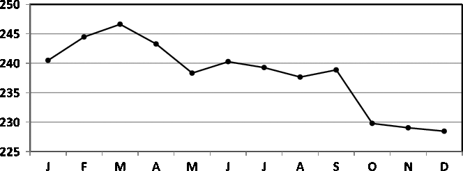
Fig. 1. Seasonality of births in Switzerland (1876–1890).
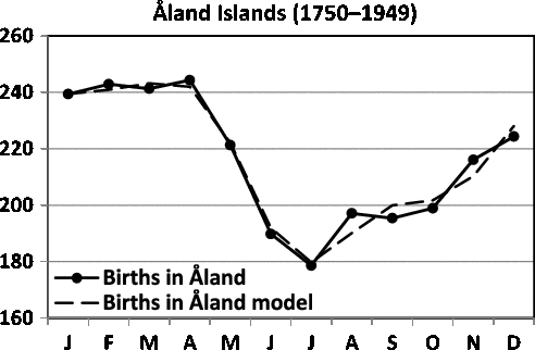
Fig. 2. Seasonality of births in Åland (Finland).

Fig. 3. Seasonality of births in Sweden for the decades 1841–1850 and 1941–1950. There are marked seasonality discrepancies between the two decades.

Fig. 4. Trends in levels of peaks of births in Sweden (1841–1950).

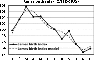
Fig. 5. Seasonality of birth data for England and Wales (1952–1975; James, Reference James1980).

Fig. 6. Seasonality of births for the USA (1985–1988; Elster & Bleyl, Reference Elster and Bleyl1991).

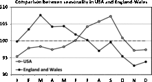
Fig. 7. Comparison between the James’ data (England and Wales) and the Elster and Bleyl data (USA). Note the strong differences in seasonality.
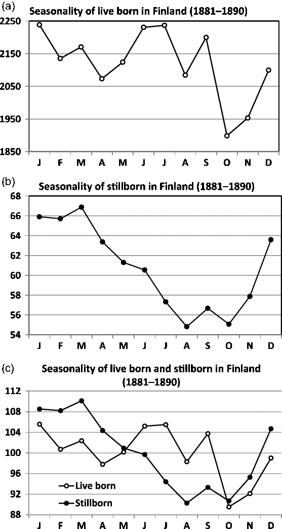
Fig. 8. Seasonality of live and stillbirths in Finland (1881–1890). The seasonality of live births is given in (a) and of stillbirths in (b). Note the marked differences in seasonality expressed in (c).
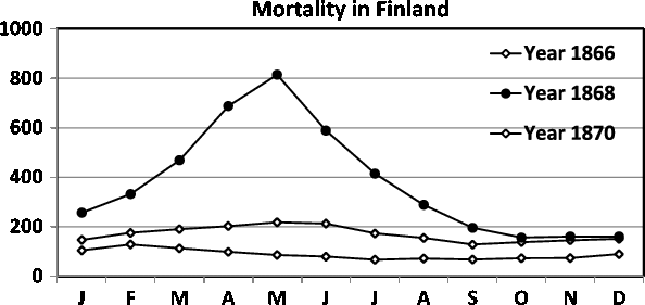
Fig. 9. Seasonality of mortality in Finland during 1866, 1868 and 1870. In 1868, the famine was exceptionally severe resulting in seasonality of mortality, with an extreme peak in the spring (April and May). For details, see the text.
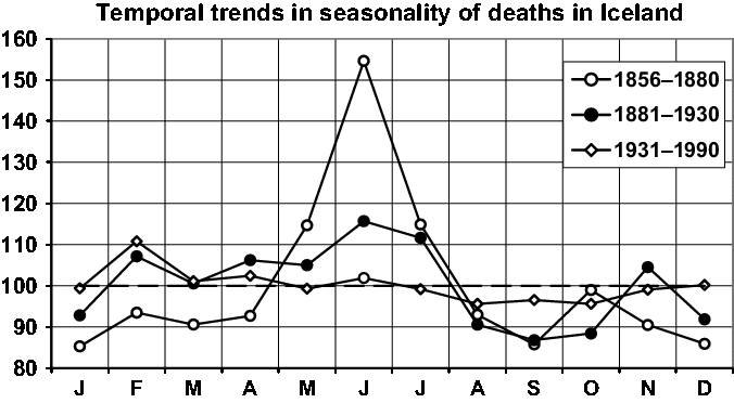
Fig. 10. Seasonality of three periods.
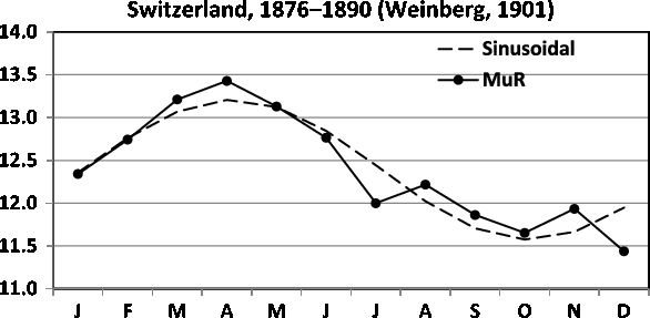
Fig. 11. Seasonality of MUR in Switzerland in 1876–1890. The obtained sinusoidal model is included.

Fig. 12. Seasonality of the TWR in Åland, 1750–1949. An acceptable sinusoidal model is included.

Fig. 13. Seasonality of triplets in the USA according to Elster and Bleyl (Reference Elster and Bleyl1991).

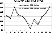
Fig. 14. Seasonality of TRR in England and Wales according to James (Reference James1980). The trigonometric regression model is included.

Fig. 15. Seasonal variation in the sex ratio observed in Åland during the centuries 1653–1750, 1751–1850 and 1851–1950. For detailed discussion, see the text.

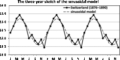
Fig. 16. Three-year sketch is based on Figure 11.
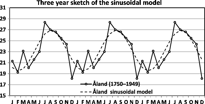
Fig. 17. Three-year sketch is based on Figure 12.
Materials
In this study, we apply the methods on various demographic seasonal data used in earlier papers. In Table 1, we present data concerning all and multiple maternities from Switzerland in 1976–1890 initially published by Weinberg (Reference Weinberg1901). Obviously, the majority of multiple maternities are twin maternities.
Table 1. Seasonality of all and multiple births in Switzerland (1876–1890) according to Weinberg (Reference Weinberg1901). Obviously, the majority of multiple maternities are twin maternities
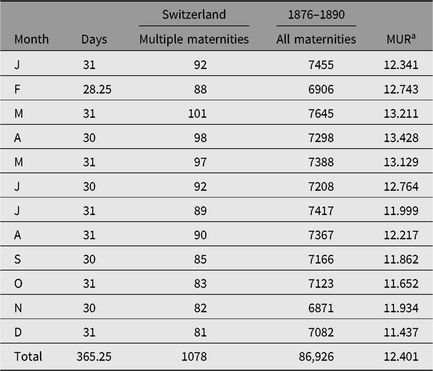
a MUR = multiple maternity rate.
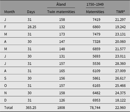
During his work on his thesis (Eriksson, Reference Eriksson1973) Aldur W. Eriksson collected a large data set concerning twinning from the Åland Islands (Finland). Later, our group (Eriksson and Fellman) continued the data collection and the obtained data sets have been a good source for our continuing twinning studies. Seasonality twinning data initially published by Eriksson (Reference Eriksson1973) are presented here in Table 2. These data, as well as the Switzerland 1976–1890 data in Table 1 from Weinberg (Reference Weinberg1901), are republished in this study because the original data may be difficult to find. Other data analyzed in this study are published in journals readily available and are therefore not republished. The seasonal data in Table 2 are used and were published in several studies by Eriksson and Fellman. These published data tables are identical and the obtained results match, but in some studies the periods presented are mistakenly different. The period 1750–1949 initially given by Eriksson (Reference Eriksson1973) is the correct one. In this study, we refer to this period.
Table 2. Seasonal twinning data for the Åland Islands (1750–1949; Eriksson, Reference Eriksson1973)
a TWR = twin maternity rate.
Results
In the following, we apply the trigonometric regression model on data concerning the demographic variables births (both live and still), deaths, twins, triplets and sex ratios.
Births
Fellman and Eriksson (Reference Fellman and Eriksson1999) have built sinusoidal and Walter–Elwood (Walter & Elwood, Reference Walter and Elwood1975) models for twinning data for Switzerland (1876–1890) and for Åland (Finland) (1750–1949; Tables 1 and 2, respectively). In this study, we build trigonometric regression models for these data and compare the results with earlier results. The seasonality of births in Switzerland and in Åland (Finland) are presented in Figures 1 and 2, respectively. In Figure 1, one can locate a peak in March and a trough in December. The long distance between the peak and the trough speaks against a sinusoidal pattern, and a trigonometric regression model should be applied. The trigonometric regression model gives a better fit, but the interpretation of the model is difficult to perform. In Figure 2, one observes the peak in April and the trough in July. Now, the distance is too short for a sinusoidal model.
The optimal regression model for births in Åland (1750–1949) is
The goodness of fit is acceptable (
![]() $$\bar R$$
2 = 0.962 and F = 70.70), but the model is difficult to interpret.
$$\bar R$$
2 = 0.962 and F = 70.70), but the model is difficult to interpret.
In Figure 3, we compare the seasonality of births in Sweden for 1841–1850 and 1941–1950. One observes that for the decade in the 19th century, there are two almost identical peaks in January and September. For the decade 1941–1950, the spring peak is increased and moved to April and the September peak is markedly decreased.
If sinusoidal models are assumed, it is the best attempt to introduce the model angle and follow its temporal trend. Alternatively, one can follow temporal trends of the troughs and peaks. For both periods in this study of the Swedish data, the two peaks indicate that a sinusoidal model is not acceptable. In Figure 4, one can follow the trends of the spring and autumn peaks. Both trends show rather constant levels of the peaks during the 19th century, but thereafter the spring peak shows a marked increase and the autumn peak shows a marked decrease.
A comparison between James’ (Reference James1980) data for England and Wales (1952–1975) and Elster and Bleyl’s (Reference Elster and Bleyl1991) data for US births (1985–1988) demands standardization of data to indices with means of 100. The regression model of the seasonality of birth data for England and Wales is
and the data are given in Figure 5. The model is significant (
![]() $$\bar R$$
2 = 0.885 and F = 22.0). The corresponding model for US birth data is
$$\bar R$$
2 = 0.885 and F = 22.0). The corresponding model for US birth data is
and the graphs are presented in Figure 6. The model is significant (F = 67.48 and
![]() $$\bar R$$
2 = 0.973).
$$\bar R$$
2 = 0.973).
The comparison between the seasonality patterns is presented in Figure 7. Note that the two data sets are obtained for comparable periods: 1952–1975 for James and 1985–1988 for Elster and Bleyl, and that the data are from countries with a similar temperate climate in the northern hemisphere (England and Wales vs. USA). Despite this, marked differences in seasonality can be observed. For the England and Wales data, we observe a maximum in the spring, in contrast to the maximum for the US data being in the autumn.
Stillbirths
A good knowledge of the seasonal variation during normal years is of fundamental importance for studies of the effects of wars, famines, epidemics or similar privations (Land & Cantor, Reference Land and Cantor1983). For the period 1881–1890 in Finland, the seasonality of live births is presented in Figure 8(a) and that of stillbirths in Figure 8(b). The comparison between the graphs demands standardized indices. Note the marked differences in the seasonality expressed in Figure 8(c).
Mortality
During the 1860s, there was a severe famine in Finland. Fellman and Eriksson (Reference Fellman and Eriksson2002) gave a thorough and detailed presentation of the demographic effects of this deprivation. In this study, we return to these austere days in Finland. We consider the seasonal variations in the mortality. The famine started in 1866, with the most severe period occurring in 1868, and the deprivation terminated in 1870. The birth rate in Finland during 1868 was only about 70% of that in normal years and showed an aberrant seasonality, with a strong trough from October 1868 to February 1869, that is, conceptions were fewer between January and May 1868, when the food shortage was extremely severe (Fellman & Eriksson, Reference Fellman and Eriksson2002).
During famines and other extreme conditions, the seasonality of mortality often shows a markedly different pattern. According to Fellman and Eriksson (Reference Fellman and Eriksson2002), as a consequence of the severe famine in Finland in 1867–1868, the mortality for the whole year in 1868 was almost four times as high as during normal years, and the seasonality of the mortality was even more accentuated. In Figure 9, we present the seasonality of the mortality in Finland during 1866, 1868 and 1870. The years 1866 and 1870 were almost normal with respect to famine, but during 1868 the famine was exceptionally hard and resulted in extreme mortality values during the spring (April and May), when the food showed the greatest deficiency before the new harvest.
Icelandic Historical Statistics (IHS, 1997) has published a long-term series concerning demographic data. Fellman and Eriksson (Reference Fellman and Eriksson2002) and Fellman (Reference Fellman2016, Reference Fellman2019) presented a detailed historic analysis of the mortality in Iceland based on the Icelandic data. They especially noted that the seasonal variation in the mortality data from Iceland, 1856–1990, shows a strong secular decrease, and the connection between this temporal trend and the epidemiological transition was considered. For this temporal finding, they analyzed and presented socioeconomic explanations and obtained interesting results (Fellman & Eriksson, Reference Fellman and Eriksson2002). They considered the mortality data from Iceland for the period 1856–1990. To obtain temporal comparisons, Fellman and Eriksson transformed the rates measuring deaths per day to indices. Figure 4 in Fellman and Eriksson (Reference Fellman and Eriksson2002) shows the time series of the seasonal indices and the annual rates of deaths per 1000. After 1856, the death rate shows a steadily decreasing trend from over 30 per thousand in the 1850s and 1860s to about 7 during the second half of the 20th century. The extreme peak for the period 1861–1870 is largely caused by an increased number of drownings and accidents of other types. In 1861–1865, the death rate in males caused by drowning was about 3 per thousand. This was followed by a clear continuous decreasing trend. At the beginning of the 20th century, the corresponding death rate was between 1 and 2 per thousand. After World War II, the decreasing trend is even more noticeable (IHS, 1997).
Omran (Reference Omran1971) proposed the epidemiological transition, consisting of three stages, and later Olshansky and Ault (Reference Olshansky and Ault1986) introduced a fourth stage. Rogers and Hackenberg (Reference Rogers and Hackenberg1987) named the fourth stage the hybristic stage and suggested that the respective turning points of the stages were 1875, 1930 and 1970. The accepted stages are: (a) age of pestilence and famine (up to 1875); (b) age of receding pandemics (1876–1930); (c) age of degenerative and man-made diseases (1931–1970); and (d) hybristic stage (1971–).
Following these stages, Fellman and Eriksson (Reference Fellman and Eriksson2002) performed a pooling of the data. They pooled the data into four subperiods: 1856–1875, 1876–1930, 1931–1970 and 1971–1990, and compared the seasonal patterns for these subperiods. A diminishing trend in the seasonality is clearly discernible. The Icelandic data for the period 1856–1875 show strong seasonal variation, with one marked mortality peak in June. During the period 1876–1930, the summer peak declined and the mortality in the winter and spring increased. A small peak is discernible in late autumn. For the period 1931–1970, the mortality values are high during the spring and early summer (peaks in February, April and June). The autumn peak, although diminished, is still discernible. This indicates further reduced seasonal variation. For the last period, 1971–1990, the seasonal variation has almost disappeared. As Fellman and Eriksson (Reference Fellman and Eriksson2002) already stressed, a specific aspect of the mortality pattern in Iceland in the 19th century is the high level of mortality caused by drowning. Being a cause of death that almost entirely affected males (over 95% of the victims were males), it is an important factor when the mortality in Iceland is studied. Figure 7 in Fellman and Eriksson (Reference Fellman and Eriksson2002) presents the mortality per 1000 for drowning and other accidents.
Although the number of drownings has decreased markedly since the 19th century, drowning was still a notable cause of death for males in the first half of the 20th century (Figure 6; Fellman & Eriksson, Reference Fellman and Eriksson2002).
In Figure 10, we give a short presentation of the central result of Fellman and Eriksson (Reference Fellman and Eriksson2002). They grouped the period 1856–1990 into three subperiods: the 19th century period, 1856–1880; the turn of the century, 1881–1930; and the recent period, 1931–1990. The temporal changes in the seasonality discussed in detail by Fellman and Eriksson (Reference Fellman and Eriksson2002) can easily be seen in Figure 10. One identifies the strong seasonality for the oldest period with the marked peak in the summer, slight seasonality during the turn of the century and the almost eliminated seasonality of today. The slight seasonality of today can be explained by the Icelandic climate, which is virtually identical for all four seasons.
Twinning
For Switzerland, the rates are according to Weinberg multiple maternity rates (MUR), but obviously twin confinements dominate these rates. Fellman (Reference Fellman2017) and Fellman and Eriksson (Reference Fellman and Eriksson1999) built sinusoidal models for the twinning rates (TWRs) for Switzerland (1876–1890) given in Table 1 and for Åland (Finland; 1750–1949) given in Table 2. In this study, we build trigonometric regression models for these data and compare the results with earlier findings. For MUR in Switzerland (1876–1890), the obtained seasonal model is a sinusoidal model Yi = 12.391 + 0.779 sin(ti) - 0.247 cos(ti) (Fellman, Reference Fellman2017; Fellman & Eriksson, Reference Fellman and Eriksson1999).
The model is significant (F = 26.72, p < .001,
![]() $$\bar R$$
2 = 0.824), and in Figure 11, one can locate a peak in April and a trough in October. The distance between the peak and the trough seems to be about six months, indicating that a sinusoidal pattern is acceptable.
$$\bar R$$
2 = 0.824), and in Figure 11, one can locate a peak in April and a trough in October. The distance between the peak and the trough seems to be about six months, indicating that a sinusoidal pattern is acceptable.
Also for Åland, the obtained seasonal model is a sinusoidal model Yi = 23.208 - 2.458 cos(ti ) - 2.738 sin(ti ) (Fellman, Reference Fellman2017; Fellman & Eriksson, Reference Fellman and Eriksson1999).
The model is significant F = 10.35, P < 0.01
![]() $$\bar R$$
2 = 0.630). In Figure 12, one observes the trough in February and a peak in July. Now the distance is acceptable for a sinusoidal pattern.
$$\bar R$$
2 = 0.630). In Figure 12, one observes the trough in February and a peak in July. Now the distance is acceptable for a sinusoidal pattern.
Triplets
Seasonality of triplets in the USA is according to Elster and Bleyl (Reference Elster and Bleyl1991) given in Figure 13. The only possible model is a multiple trigonometric regression, but it is difficult to interpret.
The seasonality of triplets in England and Wales is presented in James (Reference James1980). The only possible model for the triplet rate (TRR) index is a multiple trigonometric regression
but it is difficult to interpret. The model is significant, that is, F = 13.41 with p < .01, and
![]() $$\bar R$$
2 = 0.871.
$$\bar R$$
2 = 0.871.
Sex ratios
In this study, we also analyse the seasonal variation in the secondary sex ratio in Åland. In order to make it possible to investigate temporal effects of the seasonality, we divide the temporal data set into the subperiods 1653–1750, 1751–1850 and 1851–1950. We measured the secondary sex ratio as the proportion (%) of males. The seasonal variation shows large differences and decreasing seasonalities between the three centuries. The standard deviation is 1.382 for 1653–1750, 1.088 for 1751–1850 and 0.564 for 1851–1950. For 1653–1750, the sex ratio shows a slight increasing trend during the year. A slight similar trend can be seen during 1851–1950. For 1751–1850, such an increase is not observed, but for July, an extreme value can be noted. For 1653–1750, the overall sex ratio is 51.29, for 1751–1850 it is 51.05 and for 1851–1950 it is 51.40. No temporal trends are apparent. Figure 15 shows that no statistically significant monthly heterogeneity emerges. Using chi-squared tests with 11 degrees of freedom, we obtained nonsignificant monthly test values for all periods: 8.67 for 1653–1750, 18.61 for 1751–1850, 6.90 for 1851–1950 and 11.06 for the whole data set (the 5% critical value is 19.67).
Discussion
Fellman and Eriksson (Reference Fellman and Eriksson2000) considered monthly data and paid special attention to seasonality problems. They noted that several authors have proposed that the monthly data should be pooled to quarterly data (e.g., Nonaka & Miura, Reference Nonaka and Miura1987a, Reference Nonaka, Miura and Miura1987b). The opinion of Fellman and Eriksson (Reference Fellman and Eriksson2000) was that this should be done with great caution and tested empirically. Pooling must be based entirely on assumptions and the proposed model, but under no circumstances on the data. Furthermore, it reduces the number of observations, so that it is difficult to model the seasonal pattern statistically. In addition, pooling may mask individual months with exceptional data, for example, birth data in September (Fellman & Eriksson, Reference Fellman and Eriksson1999). They also stressed their opinion that monthly data are well suited for the study of seasonal variation. The analyses can be based on a sufficient number of time points, which may not be the case with quarterly data. If the year is split into smaller parts than months (e.g., into weeks), the seasonal pattern, especially when rare events are considered, is easily masked by random fluctuations, and the data obtained are not large enough for consistent estimates. Also, official seasonal statistics of demographic items is often based on monthly data (Fellman & Eriksson, Reference Fellman and Eriksson2000).
Bobak and Gjonca (Reference Bobak and Gjonca2001) stressed that the number of births varies markedly by season, but the causes of this variation are not fully understood. Proposed explanations include temperature or photoperiod, seasonal variation in pregnancy loss or cultural factors. In their paper, they examined whether birth seasonality is influenced by sociodemographic factors. Bobak and Gjonca used data on all live births registered in the Czech Republic in 1989–1991. Differences in the degree of seasonality between sociodemographic groups were examined by inspection of curves, by comparing coefficients of variations of monthly numbers of births and by calculating the ratios of the number of births in the three peak months (March–May) to the number of births in the three lowest months (October–December). They found large differences in the size of the seasonal variation in births by sociodemographic factors. Especially, the seasonal variation was highly pronounced in mothers who were 25–34 years old, had higher education, were married and were pregnant with their second or third child. By contrast, birth seasonality was weak in mothers who were aged below 19 years or above 35 years, were unmarried, had low education and were expecting their first or fourth or higher order birth. Furthermore, they found that in a multivariate model, all four sociodemographic variables contributed significantly to seasonal variation. Their results suggested that the seasonality of births is, in addition to climatic factors, strongly influenced by sociodemographic factors.
Gebremedhin (Reference Gebremedhin2014) compared the multiple birth rates across 12 months using a bivariate logistic regression model. However, no significant seasonal variation was observed. For Icelandic males, Fellman and Eriksson (Reference Fellman and Eriksson2002) had to include drownings as one important indicator of the harsh living conditions. In the first half of the 19th century, the fishermen had a hard life practicing their profession and braving the Atlantic storms in the small vessels of that time. Until the 20th century, the sex ratio for the Icelandic population was low relative to the sex ratio for both Norway and Sweden, indicating the greater effect of mortality from drownings and malnutrition and its sequelae on males than on females (Tomasson, Reference Tomasson1977).
Above, we have applied trigonometric regression models to different demographic variables. The results show that the models usually provided a good fit. However, when the obtained model is a multiple one, it shows complicated fluctuations. Hence, it is often difficult to interpret. The interpretation is easier when the obtained model is simpler, particularly when it is a sinusoidal one.
In Figure 16, we present a three-year sketch based on the Switzerland twinning data in Figure 11, and in Figure 17, we present a three-year sketch based on the Åland twinning data in Figure 12. The figures show the periodic fluctuations of the sinusoidal model. A sinusoidal model shows annual variation with a high and low value. Consequently, when the sinusoidal model yields a rather good fit and potential improvement is minute, the sinusoidal model is easily explained and should be used.
Financial support
This study was in part supported by a grant from the Magnus Ehrnrooths Stiftelse Foundation.

