


1 Introduction
The transcript of the talk by Donald E. Knuth titled Let’s Not Dumb Down the History of Computer Science published by ACM (2021) includes the statement:
… it would really be desirable if there were hundreds of papers on history written by computer scientists about computer science.
This quote was inspirational for this technical note devoted to a historical survey of informal semantics that are associated with logic programming under answer set semantics (in the sequel, we mostly drop under answer set semantics when referring to logic programming and logic programs).
We focus on four seminal publications and align informal semantics discussed there using the same style of presentation and propositional programs. We trust that within such settings key ideas and tangible differences between the distinct views come to the surface best. The earliest publication of the four dates back to 1988, and the latest dates back to 2014. It would seem that the subject of informal semantics is only peripheral scoring at such a low count of major references. Rather, the word informal makes this subject rare in the discussions of logic programming. Nevertheless, the 2014 reference is an introductory chapter titled Informal Semantics of the textbook on Knowledge Representation, Reasoning, and Design of Intelligent Agents by Gelfond and Kahl. The prominent position of this chapter points at the importance of the subject, especially when we consider passing on the knowledge and practice of logic programming to a broad audience.
As the presentation unfolds, a story of two views on logic programs will emerge. One view is via the prism of answer set programming (ASP) and another view is via the prism of ASP-Prolog. We reserve the term – ASP – to a constraint programming paradigm, where an ASP practitioner while coding specifications of a considered problem ensures that the solutions to this problem correspond to answer sets of the coded program (Brewka et al., Reference Brewka, Eiter and Truszczynski2011). ASP is frequently associated with solving difficult combinatorial search problems via a programming methodology of generate-define-test and underlying grounding and solving technology. The term – ASP-Prolog – is used to denote a knowledge representation language geared to model and capture domain knowledge with the underlying intelligent/rational agent in mind (Gelfond and Kahl, Reference Gelfond and Kahl2014, Section 2). One may utilize ASP-Prolog as a programming language, but may also simply use it for describing specifications without thinking about a computational task or solving this task.
This presentation of the four surveyed publications almost follows their timeline starting with the earliest work. In many places, we present the original quotes from the discussed sources to avoid misrepresentation of the originals.
2 Formal and informal semantics of basic programs by GL’88
We start by recalling the formal and informal semantics of basic logic programs as they were introduced by Gelfond and Lifschitz (Reference Gelfond, Lifschitz, Kowalski and Bowen1988).
A basic rule is an expression of the form
 \begin{equation} A \leftarrow B_1, \dots, B_n,{\mathtt{not}\;} C_1, \dots, {\mathtt{not}\;} C_m, \end{equation}
where
 $A$
,
$A$
,
 $B_i$
, and
$B_i$
, and
 $C_j$
are propositional atoms. The atom
$C_j$
are propositional atoms. The atom
 $A$
is the head of the rule and the expression
$A$
is the head of the rule and the expression
 $B_1,\ldots, B_n,{\mathtt{not}\;} C_1, \dots, {\mathtt{not}\;} C_m$
is its body. A basic (logic) program is a finite set of such rules. In the sequel, we introduce rules of somewhat different syntactic structure, yet we agree to call the left-hand side of the rule operator/connective, denoted by
$B_1,\ldots, B_n,{\mathtt{not}\;} C_1, \dots, {\mathtt{not}\;} C_m$
is its body. A basic (logic) program is a finite set of such rules. In the sequel, we introduce rules of somewhat different syntactic structure, yet we agree to call the left-hand side of the rule operator/connective, denoted by
 $\leftarrow$
, head and the right-hand side body. A rule whose body is empty
$\leftarrow$
, head and the right-hand side body. A rule whose body is empty
 $(n=m=0)$
is called a fact; in such rules connective
$(n=m=0)$
is called a fact; in such rules connective
 $\leftarrow$
is often dropped.
$\leftarrow$
is often dropped.
For a rule
 $r$
of the form (1) and a set
$r$
of the form (1) and a set
 $X$
of atoms, the reduct
$X$
of atoms, the reduct
 $r^X$
is defined whenever there is no atom
$r^X$
is defined whenever there is no atom
 $C_j$
for
$C_j$
for
 $j \in \{1,\ldots, m\}$
such that
$j \in \{1,\ldots, m\}$
such that
 $C_j \in X$
. If the reduct
$C_j \in X$
. If the reduct
 $r^X$
is defined, then it is the rule
$r^X$
is defined, then it is the rule
 \begin{equation} A \leftarrow B_1,\ldots, B_n. \end{equation}
The reduct
 $\Pi ^X$
of the program
$\Pi ^X$
of the program
 $\Pi$
consists of the rules
$\Pi$
consists of the rules
 $r^X$
for all
$r^X$
for all
 $r\in \Pi$
, for which the reduct is defined. A set
$r\in \Pi$
, for which the reduct is defined. A set
 $X$
of atoms satisfies rule (2) if
$X$
of atoms satisfies rule (2) if
 $A$
belongs to
$A$
belongs to
 $X$
or there exists
$X$
or there exists
 $i\in \{1,\dots, n\}$
such that
$i\in \{1,\dots, n\}$
such that
 $B_i\not \in X$
. We say that a set
$B_i\not \in X$
. We say that a set
 $X$
of atoms is a model of a program consisting of rules of the form (2) when
$X$
of atoms is a model of a program consisting of rules of the form (2) when
 $X$
satisfies all rules of this program. A set
$X$
satisfies all rules of this program. A set
 $X$
is a stable model/answer set of
$X$
is a stable model/answer set of
 $\Pi$
, denoted
$\Pi$
, denoted
 $X \models _{st} \Pi$
, if it is a subset minimal model of
$X \models _{st} \Pi$
, if it is a subset minimal model of
 $\Pi ^X$
; A subset minimal model is such that none of its strict subsets is also a model.
$\Pi ^X$
; A subset minimal model is such that none of its strict subsets is also a model.
Quotes by Gelfond and Lifschitz (Reference Gelfond, Lifschitz, Kowalski and Bowen1988) on Intuitive Meaning of Basic Programs (verbatim modulo names for programs and sets of atoms):
-
Quote 1: The intuitive meaning of stable setsFootnote 1 can be described in the same way as the intuition behind “stable expansions” in autoepistemic logic: they are “possible sets of beliefs that a rational agent might hold” (Moore, Reference Moore1985) given
 $\Pi$
as his premises. If
$X$
is the set of (ground) atoms that I consider true, then any rule that has a subgoal
$not\ C$
with
$C\in X$
is, from my point of view, useless; furthermore, any subgoal
$not\ C$
with
$C\not \in X$
is, from my point of view, trivial. Then I can simplify the premises
$\Pi$
and replace them by
$\Pi ^X$
. If
$X$
happens to be precisely the set of atoms that logically follow from the simplified set of premises
$\Pi ^X$
, then I am “rational”.
$\Pi$
as his premises. If
$X$
is the set of (ground) atoms that I consider true, then any rule that has a subgoal
$not\ C$
with
$C\in X$
is, from my point of view, useless; furthermore, any subgoal
$not\ C$
with
$C\not \in X$
is, from my point of view, trivial. Then I can simplify the premises
$\Pi$
and replace them by
$\Pi ^X$
. If
$X$
happens to be precisely the set of atoms that logically follow from the simplified set of premises
$\Pi ^X$
, then I am “rational”.


Later, Gelfond and Lifschitz (Reference Gelfond and Lifschitz1991) say about a basic program the following:
-
Quote 2: A “well-behaved” program has exactly one stable model, and the answer that such a program is supposed to return for a ground query
$A$
is yes or no, depending on whether
$A$
belongs to the stable model or not. (The existence of several stable models indicates that the program has several possible interpretations).


The historical roots of stable model semantics for logic programs as a formal tool for model-theoretic declarative semantics of Prolog (Kowalski, Reference Kowalski1988) are apparent in these quotes. The expectation is to consider a well-behaved program with a single stable model. Yet, the authors acknowledge the possibility of programs with several stable models that indicates that the program has several possible interpretations or induces several possible sets of beliefs. In this paper, it will prove of value to distinguish between the concepts possible interpretations and possible sets of beliefs. In 1988, these terms were used as synonyms. It is convenient to imagine that the concept of possible interpretation stands behind what we characterize here as ASP, whereas the concept of possible sets of beliefs stands behind ASP-Prolog. We now review these frameworks prior to an attempt to formalize the presented quotes that will result in what we denote as an original informal semantics of basic programs.
2.1 ASP and ASP-Prolog
2.1.1 Answer set programming
Marek and Truszczynski (Reference Marek, Truszczynski, Apt, Marek, Truszczynski and Warren1999) and Niemelä (Reference Niemelä1999) open a new era for stable model semantics by proposing the use of logic programs under this semantics as constraint programming paradigm for modeling combinatorial search problems. This marks the birth of ASP. Here is what the abstract of the paper by Marek and Truszczynski says:
-
We demonstrate that inherent features of stable model semantics naturally lead to a logic programming system that offers an interesting alternative to more traditional logic programmingFootnote 2 … The proposed approach is based on the interpretation of program clauses as constraints. In this setting programs do not describe a single intended model, but a family of stable models. These stable models encode solutions to the constraint satisfaction problem described by the program. …We argue that the resulting logic programming system is well-attuned to problems in the class NP, has a well-defined domain of applications, and an emerging methodology of programming.
In other words, Marek and Truszczynski and Niemelä propose to see logic rules of the program as specifications of the constraints of a problem at hand. Logic programming is seen as a provider of a general-purpose modeling language that supports solutions for search problems. Let us make these claims precise by considering the notion of a search problem following the lines by Brewka et al. (Reference Brewka, Eiter and Truszczynski2011). A search problem
 $P$
consists of a set of instances with each instance
$P$
consists of a set of instances with each instance
 $I$
assigned a finite set
$I$
assigned a finite set
 $S_P(I)$
of solutions. In the proposal by Marek and Truszczynski and Niemelä, to solve a search problem
$S_P(I)$
of solutions. In the proposal by Marek and Truszczynski and Niemelä, to solve a search problem
 $P$
, one constructs a logic program
$P$
, one constructs a logic program
 $\Pi _P$
that captures problem specifications so that when extended with facts
$\Pi _P$
that captures problem specifications so that when extended with facts
 $F_I$
representing an instance
$F_I$
representing an instance
 $I$
of the problem, the answer sets of
$I$
of the problem, the answer sets of
 $\Pi _P\cup F_I$
are in one-to-one correspondence with members in
$\Pi _P\cup F_I$
are in one-to-one correspondence with members in
 $S_P(I)$
. In other words, answer sets of
$S_P(I)$
. In other words, answer sets of
 $\Pi _P\cup F_I$
describe all solutions of problem
$\Pi _P\cup F_I$
describe all solutions of problem
 $P$
for the instance
$P$
for the instance
 $I$
. Thus, solving a search problem
$I$
. Thus, solving a search problem
 $P$
is reduced to finding a uniform logic program – that we denoted as
$P$
is reduced to finding a uniform logic program – that we denoted as
 $\Pi _P$
– which encodes problem’s specifications/constraints.
$\Pi _P$
– which encodes problem’s specifications/constraints.
The logic rules of the program – the key syntactic building blocks of logic programming – become the vehicles for stating constraints/specifications of a problem under consideration. A program is typically evaluated by means of a grounder-solver pair. A grounder (Syrjänen and Niemelä, Reference Syrjänen and Niemelä2001; Gebser et al., Reference Gebser, Schaub and Thiele2007; Calimeri et al., Reference Calimeri, Cozza, Ianni and Leone2008) is responsible for eliminating first-order variables occurring in a logic program in favor of suitable object constants resulting in a propositional program – atoms of such programs are called ground. An answer set solver – a system in the spirit of SAT solvers (see, e.g. (Lierler, Reference Lierler2017)) – is responsible for computing answer sets (solutions) of a program. Let us draw a parallel with Prolog. In Prolog (Kowalski, Reference Kowalski1988), a single intended model is assigned to a logic program. The SLD-resolution (Kowalski, Reference Kowalski and Rosenfeld1974) is at the heart of the control mechanism behind Prolog implementations. Together with a logic program, a Prolog system expects a query (possibly multiple queries). This query is then evaluated by means of SLD-resolution and a given program against an intended model. Thus, even though Prolog and ASP share the basic language of logic programs, their programming methodologies and underlying solving/control technologies are different.Footnote 3
2.1.2 ASP programming methodology
Eiter et al. (Reference Eiter, Faber, Leone, Pfeifer and Minker2000) illustrate how logic programs under answer set semantics can be used to encode problems in a highly declarative fashion, following a “Guess&Check” paradigm. We restate this paradigm verbatim utilizing the terminology of search problem and its instance introduced before.
-
Given a set
$F_I$
of facts that specify an instance
$I$
of some problem
$P$
, a Guess&Check program
$\Pi$
for
$P$
consists of the following two parts -
Guessing Part: The guessing part
$G\subseteq \Pi$
of the program defines the search space, in a way such that answer sets of
$G\cup F_I$
represent “solution candidates” for
$I$
. -
Checking Part: The checking part
$C\subseteq \Pi$
of the program tests whether a solution candidate is in fact a solution, such that the answer sets
$G\cup C \cup F_I$
represent the solutions of the problem instance
$I$
.


Eiter et al. point at a close relation of the Guess&Check approach with the generate-and-test paradigm in the AI community (Winston, Reference Winston1992).
Lifschitz (Reference Lifschitz2002) refines the Guess&Check approach and coins a term generate-define-test for this emerging methodology in logic programming that splits program rules into three groups:
-
• the generate group is responsible for defining a large class of “potential solutions”
-
• the test group is responsible for stating conditions to weed out potential solutions that do not satisfy the problem’s specifications; and
-
• the define group is responsible for defining concepts that are essential in stating the conditions of generate and test.
In this work, “the idea of ASP is to represent a given computational problem by a program whose answer sets correspond to solutions, and then use an answer set solver to find a solution”. The paper illustrates the use of ASP to solve a sample planning problem. Yet, there are no references to how one would intuitively read, for example, an occurrence of atom
 $A$
or expression
$A$
or expression
 $not\ A$
in rules. This is also true of many other instances of papers describing various applications of ASP.
$not\ A$
in rules. This is also true of many other instances of papers describing various applications of ASP.
To the best of our knowledge, Denecker et al. (Reference Denecker, Lierler, Truszczyński and Vennekens2012) in addition to earlier reviewed quotes in this section are the two major accounts for reconciling the use of ASP (not ASP-Prolog) in practice and intuitive readings of answer sets and rules of programs. The previous to the last section reviews an account by Denecker et al., while the remainder of this section predominantly concerns making already reviewed quotes more precise.
2.1.3 ASP-prolog
We reviewed the concept of ASP as championed by Marek and Truszczynski (Reference Marek, Truszczynski, Apt, Marek, Truszczynski and Warren1999) and Niemelä (Reference Niemelä1999). In this view, a search problem at hand is a center piece. An ability to model a considered search problem by means of a logic program so that the answer sets of this program are in one-to-one correspondence to the problem’s solutions constitutes this paradigm.
The textbook by Gelfond and Kahl (Reference Gelfond and Kahl2014) focuses on an alternative practice of logic programming under answer set semantics. It champions a view on answer sets as possible sets of beliefs. Interpreting answer sets as such implies the presence of an intelligent agent behind a program. The program itself is seen to represent a knowledge base of this agent. This corresponds to the view of a logic program as a knowledge representation and reasoning formalism for the design of intelligent agents. This is largely a position advocated in the Gelfond and Kahl textbook. We use the term ASP-Prolog to denote such use of logic programs. It makes sense to reflect on the notion of an intelligent agent provided in Section 1.1 of the cited textbook:
-
In this book when we talk about an agent, we mean an entity that observes and acts on an environment and directs its activity toward achieving goals. Note that this definition allows us to view the simplest programs as agents. A program usually gets information from the outside world, performs an appointed reasoning task, and acts on the outside world, say by printing the output, making the next chess move, starting a car, or giving advice. If the reasoning tasks that an agent performs are complex and lead to nontrivial behavior, we call it intelligent.
Brief discussions by Gelfond and Lifschitz (Reference Gelfond and Lifschitz1991) and Section 2.2.1 of the mentioned textbook are major two accounts that speak of intuitive readings of answer sets and rules of programs when ASP-Prolog is used in practice. Sections 3 and 4 of this note are devoted to these accounts.
2.2 “Formalizing” quotes 1 and 2 or informal semantics of basic programs by GL’88
Before we attempt to make the claims of Quote 1 by Gelfond and Lifschitz (Reference Gelfond, Lifschitz, Kowalski and Bowen1988) precise it is due to discuss three interrelated and yet different concepts and how we understand them within this note:
-
• a state of affairs,
-
• a belief state, and
-
• a set of beliefs/belief set.
The following example is our key vehicle in this discussion.
Example 1. Consider a toy world with four possible states of affairs that fully describe it:

A belief state is associated with/represented by a conglomeration of states of affairs. In other words, a belief state assumes that multiple states of affairs can be deemed as possible by an agent. Thus, a belief state is often associated with an agent who has partial knowledge of the world.
Returning to our toy world, the powerset of the listed four states of affairs forms the set of belief states for an agent operating in this world. For example, if an agent assumes a belief state consisting of states 1, 2, 3, 4 of affairs – let us denote it as
 $bs_1$
–, we may conclude that this agent deems everything possible (or knows nothing factual about the world). If an agent assumes a belief state consisting of states 1 and 2 of affairs – let us denote it as
$bs_1$
–, we may conclude that this agent deems everything possible (or knows nothing factual about the world). If an agent assumes a belief state consisting of states 1 and 2 of affairs – let us denote it as
 $bs_2$
–, we may conclude that this agent is aware of the fact that Mary is a student, whereas John may or may not be a student. In turn, if an agent assumes a belief state consisting of a single state 1 – let us denote it as
$bs_2$
–, we may conclude that this agent is aware of the fact that Mary is a student, whereas John may or may not be a student. In turn, if an agent assumes a belief state consisting of a single state 1 – let us denote it as
 $bs_3$
–, then we may conclude that this agent is aware of the two facts: Mary is a student and John is a student.
$bs_3$
–, then we may conclude that this agent is aware of the two facts: Mary is a student and John is a student.
We now connect the concepts of a belief set (or, a set of beliefs) and a belief state. The former is an abstraction of the latter. In other words, we understand belief sets as entities that capture/encode belief states. This encoding may lose some information so that multiple belief states may be “consistent” with a single belief set. For instance, in the context of our toy world, a belief set consisting of a single proposition Mary is a student is consistent with any belief state that contains either state 1 of affairs or state 2 of affairs. Note how this belief set cannot distinguish between these different belief states. Indeed, a belief set consisting of a single proposition Mary is a student cannot distinguish between belief states
 $bs_1$
,
$bs_1$
,
 $bs_2$
, and
$bs_2$
, and
 $bs_3$
.
$bs_3$
.
We are now ready to return to the claims of Quote 1 by Gelfond and Lifschitz (Reference Gelfond, Lifschitz, Kowalski and Bowen1988) and attempt to make these precise with the allowance that programs with multiple answer sets that correspond to possible sets of beliefs/possible interpretations are as valid programs as so-called well-behaved programs. In other words, per Quote 1 each answer set represents a set of beliefs of a rational agent (or
 $I$
); thus this agent may have multiple sets of beliefs. In the sequel, we drop the reference to “or I” and use “an agent” in the discourse.Footnote
4
In the case of basic programs, we take an understanding that
$I$
); thus this agent may have multiple sets of beliefs. In the sequel, we drop the reference to “or I” and use “an agent” in the discourse.Footnote
4
In the case of basic programs, we take an understanding that
This understanding is consistent with the view by Gelfond and Lifschitz, which is reiterated in Quote 4 in Section 3.
Claim (3) on the interpretation of answer sets has profound ramifications. Namely, this claim makes the three concepts — a state of affairs, a belief state, and a set of beliefs/belief set — exemplified earlier by highlighting their differences collapse into a single entity. Let us use an example to illustrate this point.
Example 2. Recall the toy world from Example 1. Let us take atoms
 $student(mary)$
and
$student(mary)$
and
 $student(john)$
to represent propositions Mary is a student and John is a student, respectively. If our signature of discourse is composed only of these two atoms, we can construct four distinct subsets of atoms within this signature, namely,
$student(john)$
to represent propositions Mary is a student and John is a student, respectively. If our signature of discourse is composed only of these two atoms, we can construct four distinct subsets of atoms within this signature, namely,
 \begin{equation} \{student(mary),\,\,student(john)\};\,\, \{student(mary)\};\,\, \{student(john)\};\,\, \emptyset . \end{equation}
Each of these sets of atoms can be identified in a natural manner with one of the four states of affairs that capture our toy world from Example 1 Footnote 5 ; below we rewrite the table presented in that example by substituting propositions depicting distinct states of affairs with the respective sets of atoms:

Alternatively, let us take sets listed in (4) to represent distinct belief states under the assumption that any atom not listed explicitly in a set under consideration is considered to be false. Thus, the belief state
 $\{student(mary),\,\,student(john)\}$
represents a belief state consisting of a single state of affairs denoted by 1 and represented by the same set of atoms as illustrated above; belief state
$\{student(mary),\,\,student(john)\}$
represents a belief state consisting of a single state of affairs denoted by 1 and represented by the same set of atoms as illustrated above; belief state
 $\{student(mary)\}$
represents a belief state consisting of a single state of affairs denoted by 2 and represented by the same set of atoms. The same observation holds for the remaining two belief states depicted by sets of atoms in (4). Thus, given the considered settings we may identify belief states and states of affairs. The same argument applies to the concept of a belief set.
$\{student(mary)\}$
represents a belief state consisting of a single state of affairs denoted by 2 and represented by the same set of atoms. The same observation holds for the remaining two belief states depicted by sets of atoms in (4). Thus, given the considered settings we may identify belief states and states of affairs. The same argument applies to the concept of a belief set.
We denote the informal semantics for basic programs as
 $\mathscr{G}_{\mathbb{I}}$
, where
$\mathscr{G}_{\mathbb{I}}$
, where
 $\mathbb{I}$
stands for intended interpretations of the program’s propositional atoms. It is typical in the informal semantics for classical logic expressions that each atom
$\mathbb{I}$
stands for intended interpretations of the program’s propositional atoms. It is typical in the informal semantics for classical logic expressions that each atom
 $A$
has an intended interpretation,
$A$
has an intended interpretation,
 $\mathbb{I}(A)$
, which is represented linguistically as a noun phrase about the application domain. The informal semantics
$\mathbb{I}(A)$
, which is represented linguistically as a noun phrase about the application domain. The informal semantics
 $\mathscr{G}_{\mathbb{I}}$
consists of three components:
$\mathscr{G}_{\mathbb{I}}$
consists of three components:
-
• the interpretation of structures – here, answer sets – denoted by
$\mathscr{G}_{\mathbb{I}}{\mathbb{S}}$
, -
• the interpretation of syntactical expressions in a program, denoted by
$\mathscr{G}_{\mathbb{I}}^{\mathbb{L}}$
, and -
• the interpretation of the semantic relation – here, satisfaction – denoted by
$\mathscr{G}_{\mathbb{I}}^{\models }$
.


The first component determines a function from an answer set/a set of beliefs encoded by a set
 $X$
of atoms to a belief state of some agent (or, a state of affairs). The second component determines the informal reading of syntactical expressions in a program. The third component determines the informal reading of the satisfaction relation.
$X$
of atoms to a belief state of some agent (or, a state of affairs). The second component determines the informal reading of syntactical expressions in a program. The third component determines the informal reading of the satisfaction relation.
In the view of informal semantics
 $\mathscr{G}_{\mathbb{I}}$
, an answer set encodes a belief state of some agent (or, a state of affairs – as we have seen earlier, these concepts are indistinguishable under claim (3)). To reiterate, An agent in some belief state – represented by a set
$\mathscr{G}_{\mathbb{I}}$
, an answer set encodes a belief state of some agent (or, a state of affairs – as we have seen earlier, these concepts are indistinguishable under claim (3)). To reiterate, An agent in some belief state – represented by a set
 $X$
of atoms – considers the set of all atoms in
$X$
of atoms – considers the set of all atoms in
 $X$
to be the case (believes in them), whereas any atom that does not belong to
$X$
to be the case (believes in them), whereas any atom that does not belong to
 $X$
is believed to be false by the agent, that is is not the case. Thus, we may explain the meaning of a program in terms of what atoms an agent with its knowledge of the application domain encoded as the program believes as true and what atoms an agent believes as false. Generally, an agent in some belief state considers certain states of affairs as possible and others as impossible. For basic programs, set
$X$
is believed to be false by the agent, that is is not the case. Thus, we may explain the meaning of a program in terms of what atoms an agent with its knowledge of the application domain encoded as the program believes as true and what atoms an agent believes as false. Generally, an agent in some belief state considers certain states of affairs as possible and others as impossible. For basic programs, set
 $X$
of atoms defines a unique state of affairs that the agent regards as possible in a belief state that
$X$
of atoms defines a unique state of affairs that the agent regards as possible in a belief state that
 $X$
represents. Thus, we may identify any belief state captured by
$X$
represents. Thus, we may identify any belief state captured by
 $X$
with this state of affairs. We denote a state of affairs captured by a set
$X$
with this state of affairs. We denote a state of affairs captured by a set
 $X$
of atoms under an intended interpretation
$X$
of atoms under an intended interpretation
 $\mathbb{I}$
as
$\mathbb{I}$
as
 $\mathscr{G}_{\mathbb{I}}^{\mathbb{S}}(X)$
. Table 1 summarizes a role of an answer set as a state of affairs in the considered view.
$\mathscr{G}_{\mathbb{I}}^{\mathbb{S}}(X)$
. Table 1 summarizes a role of an answer set as a state of affairs in the considered view.
Example 3. Consider a set of beliefs encoded as a set
 \begin{equation} X=\{student(mary),\,\,male(john)\} \end{equation}
of atoms under the obvious intended interpretation
 $\mathbb{I}$
for the propositional atoms in
$\mathbb{I}$
for the propositional atoms in
 $X$
. This
$X$
. This
 $X$
represents a state of affairs in which the agent considers that both statements Mary is a student and John is a male are true. At the same time, the agent considers any other statements, including John is a student and Mary is a male, false. The
$X$
represents a state of affairs in which the agent considers that both statements Mary is a student and John is a male are true. At the same time, the agent considers any other statements, including John is a student and Mary is a male, false. The
 $\mathscr{G}_{\mathbb{I}}^{\mathbb{S}}(X)$
component of informal semantics of basic programs provides us with this understanding of set
$\mathscr{G}_{\mathbb{I}}^{\mathbb{S}}(X)$
component of informal semantics of basic programs provides us with this understanding of set
 $X$
.
$X$
.
Table 1. The Gelfond-Lifschitz (Reference Gelfond, Lifschitz, Kowalski and Bowen1988) informal semantics of answer sets – sets of atoms

Table 2. The Gelfond-Lifschitz (Reference Gelfond, Lifschitz, Kowalski and Bowen1988) informal semantics for basic logic programs

Table 2 shows the Gelfond-Lifschitz (Reference Gelfond, Lifschitz, Kowalski and Bowen1988) informal semantics
 $\mathscr{G}_{\mathbb{I}}^{\mathbb{L}}$
of syntactic elements of programs. The term material implication used within the table assumes the conformance to the usual truth table of implication and thus a conditional statement can be identified with a disjunction in which the antecedent of the conditional statement is negated. As it is clear from this table, under
$\mathscr{G}_{\mathbb{I}}^{\mathbb{L}}$
of syntactic elements of programs. The term material implication used within the table assumes the conformance to the usual truth table of implication and thus a conditional statement can be identified with a disjunction in which the antecedent of the conditional statement is negated. As it is clear from this table, under
 $\mathscr{G}_{\mathbb{I}}^{\mathbb{L}}$
, extended logic programs have both classical and non-classical connectives.Footnote
6
On the one hand, the comma connective (appearing in the body of rules) is classical conjunction and the rule connective
$\mathscr{G}_{\mathbb{I}}^{\mathbb{L}}$
, extended logic programs have both classical and non-classical connectives.Footnote
6
On the one hand, the comma connective (appearing in the body of rules) is classical conjunction and the rule connective
 $\leftarrow$
is the classical implication. Note that such reading of the comma connective and the rule connective allows us to identify the empty body of the rule with
$\leftarrow$
is the classical implication. Note that such reading of the comma connective and the rule connective allows us to identify the empty body of the rule with
 $\top$
– a propositional constant whose value is always interpreted as true – and a rule with an empty body with a simple propositional statement that contains only head of this rule. Not surprisingly such rules are typically denoted as facts. On the other hand, the implicit composition operator (constructing a program out of individual rules) is non-classical because it performs a closure operation (resulting in the implementation of closed world assumption – presumption that what is not currently known to be true is false): only what is explicitly stated is known. To summarize, Table 2 is devoted to the interpretation of syntactical expressions in a program allowing us to “translate” its syntactic elements and the program itself into natural language expressions. For instance, take
$\top$
– a propositional constant whose value is always interpreted as true – and a rule with an empty body with a simple propositional statement that contains only head of this rule. Not surprisingly such rules are typically denoted as facts. On the other hand, the implicit composition operator (constructing a program out of individual rules) is non-classical because it performs a closure operation (resulting in the implementation of closed world assumption – presumption that what is not currently known to be true is false): only what is explicitly stated is known. To summarize, Table 2 is devoted to the interpretation of syntactical expressions in a program allowing us to “translate” its syntactic elements and the program itself into natural language expressions. For instance, take
 $\mathbb{I}$
to be an identity function and consider a simple programFootnote
7
$\mathbb{I}$
to be an identity function and consider a simple programFootnote
7

The annotations to the right are warranted by
 $\mathscr{G}_{\mathbb{I}}^{\mathbb{L}}$
presented in Table 2. Table 3 presents the final component
$\mathscr{G}_{\mathbb{I}}^{\mathbb{L}}$
presented in Table 2. Table 3 presents the final component
 $\mathscr{G}_{\mathbb{I}}^{\models _{st}}$
of the
$\mathscr{G}_{\mathbb{I}}^{\models _{st}}$
of the
 $\mathscr{G}_{\mathbb{I}}$
informal semantics. In the context of the simple program used to illustrate the findings presented in Table 2, the findings of Table 3 suggest that the only answer set of this program
$\mathscr{G}_{\mathbb{I}}$
informal semantics. In the context of the simple program used to illustrate the findings presented in Table 2, the findings of Table 3 suggest that the only answer set of this program
 $\{p(b),\,\, q(a)\}$
is a state of affairs inferred from the knowledge encoded in this program so that both
$\{p(b),\,\, q(a)\}$
is a state of affairs inferred from the knowledge encoded in this program so that both
 $p(b)$
and
$p(b)$
and
 $q(a)$
are the case and no other proposition is the case.
$q(a)$
are the case and no other proposition is the case.
Table 3. The Gelfond-Lifschitz (Reference Gelfond, Lifschitz, Kowalski and Bowen1988) informal semantics for the satisfaction relation

3 Formal and informal semantics of extended programs by GL’91
Here, we recall the formal and informal semantics of extended logic programs by Gelfond and Lifschitz (Reference Gelfond and Lifschitz1991). An alternative view of the informal semantics for extended logic programs is provided in (Gelfond and Kahl, Reference Gelfond and Kahl2014, Section 2.2.1) reviewed next.
A literal is either an atom
 $A$
or an expression
$A$
or an expression
 $\neg A$
, where
$\neg A$
, where
 $A$
is an atom. An extended rule is an expression of the form (1), where
$A$
is an atom. An extended rule is an expression of the form (1), where
 $A$
,
$A$
,
 $B_i$
, and
$B_i$
, and
 $C_j$
are propositional literals. An extended program is a finite set of extended rules. Gelfond and Lifschitz (Reference Gelfond and Lifschitz1991) also considered disjunctive rules of the form
$C_j$
are propositional literals. An extended program is a finite set of extended rules. Gelfond and Lifschitz (Reference Gelfond and Lifschitz1991) also considered disjunctive rules of the form
 $D_1\ or\ \dots \ or\ D_l \leftarrow B_1, \dots, B_n,{\mathtt{not}\;} C_1, \dots, {\mathtt{not}\;} C_m,$
where
$D_1\ or\ \dots \ or\ D_l \leftarrow B_1, \dots, B_n,{\mathtt{not}\;} C_1, \dots, {\mathtt{not}\;} C_m,$
where
 $D_k$
,
$D_k$
,
 $B_i$
, and
$B_i$
, and
 $C_j$
are propositional literals. Yet, the discussion of such rules is outside the scope of this note.
$C_j$
are propositional literals. Yet, the discussion of such rules is outside the scope of this note.
A consistent set of propositional literals is a set that does not contain both
 $A$
and its complement
$A$
and its complement
 ${\neg }A$
for any atom
${\neg }A$
for any atom
 $A$
. A believed literal set
$A$
. A believed literal set
 $X$
is a consistent set of propositional literals. A believed literal set
$X$
is a consistent set of propositional literals. A believed literal set
 $X$
satisfies an extended rule
$X$
satisfies an extended rule
 $r$
of the form (1) if
$r$
of the form (1) if
 $A$
belongs to
$A$
belongs to
 $X$
or there exists an
$X$
or there exists an
 $i \in \{1,\ldots, n\}$
such that
$i \in \{1,\ldots, n\}$
such that
 $B_i \not \in X$
or a
$B_i \not \in X$
or a
 $j \in \{1,\ldots, m\}$
such that
$j \in \{1,\ldots, m\}$
such that
 $C_j \in X$
. A believed literal set is a model of a program
$C_j \in X$
. A believed literal set is a model of a program
 $\Pi$
if it satisfies all rules in
$\Pi$
if it satisfies all rules in
 $\Pi$
. For a rule
$\Pi$
. For a rule
 $r$
of the form (1) and a believed literal set
$r$
of the form (1) and a believed literal set
 $X$
, the reduct
$X$
, the reduct
 $r^X$
is defined whenever there is no literal
$r^X$
is defined whenever there is no literal
 $C_j$
for
$C_j$
for
 $j \in \{1,\ldots, m\}$
such that
$j \in \{1,\ldots, m\}$
such that
 $C_j \in X$
. If the reduct
$C_j \in X$
. If the reduct
 $r^X$
is defined, then it is the extended rule of the form (2). The reduct
$r^X$
is defined, then it is the extended rule of the form (2). The reduct
 $\Pi ^X$
of the program
$\Pi ^X$
of the program
 $\Pi$
consists of the rules
$\Pi$
consists of the rules
 $r^X$
for all
$r^X$
for all
 $r\in \Pi$
, for which the reduct is defined. A believed literal set
$r\in \Pi$
, for which the reduct is defined. A believed literal set
 $X$
is an answer set of
$X$
is an answer set of
 $\Pi$
, denoted
$\Pi$
, denoted
 $X \models _{st} \Pi$
, if it is a subset minimal model of
$X \models _{st} \Pi$
, if it is a subset minimal model of
 $\Pi ^X$
. (A subset minimal model is such that none of its strict subsets is also a model.)
$\Pi ^X$
. (A subset minimal model is such that none of its strict subsets is also a model.)
Quotes by Gelfond and Lifschitz (Reference Gelfond and Lifschitz1991) on Intuitive Meaning of Extended Programs
-
Quote 3: For an extended program, we will define when a set
$X$
of ground literals qualifies as its answer set. …A “well-behaved” extended program has exactly one answer set, and this set is consistent. The answer that the program is supposed to return to a ground query
$A$
is yes, no, or unknown, depending on whether the answer set contains
$A$
,
$\neg A$
, or neither. The answer no corresponds to the presence of explicit negative information in the program.Consider, for instance, the extended program
$\Pi _1$
consisting of just one rule:Intuitively, this rule means: “
\begin{equation*}\neg q\leftarrow not\ p.\end{equation*}
$q$
is false, if there is no evidence that
$p$
is true.” We will see that the only answer set of this program is
$\{\neg q\}$
. The answers that the program should give to the queries
$p$
and
$q$
are, respectively unknown and false.
As another example, compare two programs that do not contain not:
… Thus our semantics is not “contrapositive” with respect to
\begin{equation*} \neg p\leftarrow, \ \ \ p\leftarrow \neg q\quad \hbox { and }\quad \neg p\leftarrow, \ \ \ q\leftarrow \neg p \end{equation*}
$\leftarrow$
and
$\neg$
; it assigns different meanings to the rules
$p\leftarrow \neg q$
and
$q\leftarrow \neg p$
. The reason is that it interprets expressions like these as inference rules, rather than conditionals.


This quote echos Quote 2 about basic programs: the notion of a well-behaved program resurfaces. In comparison to basic programs, extended programs provide us with a new possibility to answer queries against a program — namely, unknown. The following quote echos Quote 1 about basic programs:
-
The answer sets of
$\Pi$
are, intuitively, possible sets of beliefs that a rational agent may hold on the basis of information expressed by the rules of
$\Pi$
. If
$X$
is the set of (ground) literals that the agent believes to be true, then any rule that has a subgoal not L with
$L\in X$
will be of no use to him, and he will view any subgoal not L with
$L\not \in X$
as trivial. Thus he will be able to replace the set of rules
$\Pi$
by the simplified set of rules
$\Pi ^X$
. If the answer set of
$\Pi ^X$
coincides with
$X$
, then the choice of
$X$
as the set of beliefs is “rational”.


The following quote states the precise relationship between basic and extended programs:Footnote 8
-
Quote 4: the semantics of extended programs applied to basic programs turns into the stable model semantics. But there is one essential difference: The absence of an atom
$A$
in a stable model of a basic program represents the fact that
$A$
is false; the absence of
$A$
and
$\neg A$
in an answer set of an extended program is taken to mean that nothing is known about
$A$
.


In the section on Representing Knowledge Using Classical Negation, Gelfond and Lifschitz (Reference Gelfond and Lifschitz1991) say
-
The difference between not p and
$\neg p$
in a logic program is essential whenever we cannot assume that the available positive information about
$p$
is complete, that is when the “closed world assumption” [Reiter, 1978] is not applicable to
$p$
. The closed world assumption for a predicate
$p$
can be expressed in the language of extended programs by the ruleWhen this rule is included in the program,
\begin{equation*} \neg p\leftarrow {\mathtt {not}\;} p \end{equation*}
$not\ p$
and
$\neg p$
can be used interchangeably in the bodies of other rules. Otherwise, we use not p to express that
$p$
is not known to be true, and
$\neg p$
to express that
$p$
is false.


To summarize, Gelfond and Lifschitz describe informal semantics for extended programs based on epistemic notions of default and autoepistemic reasoning. We now present the informal semantics
 $\mathscr{GL}_{\mathbb{I}}$
for extended programs just as we presented
$\mathscr{GL}_{\mathbb{I}}$
for extended programs just as we presented
 $\mathscr{G}_{\mathbb{I}}$
for basic programs. This presentation at times (in particular, Example4) follows the lines by Denecker et al. (Reference Denecker, Lierler, Truszczynski and Vennekens2019).
$\mathscr{G}_{\mathbb{I}}$
for basic programs. This presentation at times (in particular, Example4) follows the lines by Denecker et al. (Reference Denecker, Lierler, Truszczynski and Vennekens2019).
We begin by discussing a crucial difference between
 $\mathscr{G}_{\mathbb{I}}$
and
$\mathscr{G}_{\mathbb{I}}$
and
 $\mathscr{GL}_{\mathbb{I}}$
. Informal semantics
$\mathscr{GL}_{\mathbb{I}}$
. Informal semantics
 $\mathscr{GL}_{\mathbb{I}}$
views a believed literal set
$\mathscr{GL}_{\mathbb{I}}$
views a believed literal set
 $X$
as an abstraction of a belief state (in fact, of a class of belief states that it cannot distinguish) of some agent;
$X$
as an abstraction of a belief state (in fact, of a class of belief states that it cannot distinguish) of some agent;
 $\mathscr{G}_{\mathbb{I}}$
views a set
$\mathscr{G}_{\mathbb{I}}$
views a set
 $X$
of atoms as a state of affairs. The change from “sets of atoms” to “sets of literals” and the elimination of Assumption (3) are crucial. Recall how an agent in some belief state considers certain states of affairs as possible and others as impossible. Within
$X$
of atoms as a state of affairs. The change from “sets of atoms” to “sets of literals” and the elimination of Assumption (3) are crucial. Recall how an agent in some belief state considers certain states of affairs as possible and others as impossible. Within
 $\mathscr{G}_{\mathbb{I}}$
, set
$\mathscr{G}_{\mathbb{I}}$
, set
 $X$
of atoms ends up representing a unique possible state of affairs associated with a belief state so that we may identify these two concepts. Yet, believed literal set
$X$
of atoms ends up representing a unique possible state of affairs associated with a belief state so that we may identify these two concepts. Yet, believed literal set
 $X$
is the set of all literals
$X$
is the set of all literals
 $L$
that the agent believes in, that is, those that are true in all states of affairs that the agent regards as possible. Importantly, it is not the case that a literal
$L$
that the agent believes in, that is, those that are true in all states of affairs that the agent regards as possible. Importantly, it is not the case that a literal
 $L$
that does not belong to
$L$
that does not belong to
 $X$
is believed to be false by the agent. Rather, it is not believed by the agent or as stated in Quote 4 nothing is known about
$X$
is believed to be false by the agent. Rather, it is not believed by the agent or as stated in Quote 4 nothing is known about
 $L$
to the agent. Denecker et al. (Reference Denecker, Lierler, Truszczynski and Vennekens2019) take the following interpretation of a statement literal
$L$
to the agent. Denecker et al. (Reference Denecker, Lierler, Truszczynski and Vennekens2019) take the following interpretation of a statement literal
 $L$
is not believed by an agent/nothing is known about
$L$
is not believed by an agent/nothing is known about
 $L$
: literal
$L$
: literal
 $L$
is false in some states of affairs the agent holds possible, and
$L$
is false in some states of affairs the agent holds possible, and
 $L$
must be true in at least one of the agent’s possible states of affairs (unless the agent believes the complement of
$L$
must be true in at least one of the agent’s possible states of affairs (unless the agent believes the complement of
 $L$
). This note adopts such an interpretation. We denote the class of informal belief states that are abstracted to a given formal believed literal set
$L$
). This note adopts such an interpretation. We denote the class of informal belief states that are abstracted to a given formal believed literal set
 $X$
under an intended interpretation
$X$
under an intended interpretation
 $\mathbb{I}$
as
$\mathbb{I}$
as
 $\mathscr{GL}_{\mathbb{I}}^{\mathbb{S}}(X)$
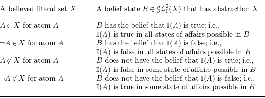
. Table 4 summarizes a view on a believed literal set as an abstraction of a belief state of some agent.
$\mathscr{GL}_{\mathbb{I}}^{\mathbb{S}}(X)$
. Table 4 summarizes a view on a believed literal set as an abstraction of a belief state of some agent.
Table 4. The Gelfond-Lifschitz (1991) informal semantics of answer sets – sets of literals
Example 4. We may view this example as a continuation of Example 3. Here we consider what would seem the same belief set but change the perspective on it from the point of view of informal semantics of basic programs to that of extended programs. Consider believed literal set (5) under the obvious intended interpretation
 $\mathbb{I}$
for the elements in
$\mathbb{I}$
for the elements in
 $X$
. This
$X$
. This
 $X$
is the abstraction of any belief state in which the agent believes that Mary is a student and John is a male, and nothing is known about such statements as John is a student or Mary is a male. One such belief state is the state
$X$
is the abstraction of any belief state in which the agent believes that Mary is a student and John is a male, and nothing is known about such statements as John is a student or Mary is a male. One such belief state is the state
 $B_0$
in which the agent considers the following states of affairs as possible:
$B_0$
in which the agent considers the following states of affairs as possible:
-
1. John is the only male in the domain of discourse; Mary is the only student.
-
2. John and Mary are both male students.
-
3. John and Mary are both male; Mary is the only student.
-
4. John is the only male; John and Mary are both students.
Another belief state corresponding to
 $X$
is the state
$X$
is the state
 $B_1$
in which the agent considers the states of affairs 2–4 of
$B_1$
in which the agent considers the states of affairs 2–4 of
 $B_0$
as possible. Indeed, for each of these belief states, it holds that Mary is a student and John is a male in all possible states of affairs of that belief state. Thus, each of the literals in
$B_0$
as possible. Indeed, for each of these belief states, it holds that Mary is a student and John is a male in all possible states of affairs of that belief state. Thus, each of the literals in
 $X$
is believed in each of the belief states
$X$
is believed in each of the belief states
 $B_0$
and
$B_0$
and
 $B_1$
. On the other hand, John is a student precisely in the state of affairs 2 and 4; Mary is a male in the states of affairs 2 and 3. Hence, literals
$B_1$
. On the other hand, John is a student precisely in the state of affairs 2 and 4; Mary is a male in the states of affairs 2 and 3. Hence, literals
 $\neg student(john)$
and
$\neg student(john)$
and
 $\neg male(mary)$
are not believed in either of the two belief states
$\neg male(mary)$
are not believed in either of the two belief states
 $B_0$
and
$B_0$
and
 $B_1$
.
$B_1$
.
The component
 $\mathscr{GL}_{\mathbb{I}}^{\mathbb{L}}$
captures the informal readings of the connectives of the informal semantics of extended programs by Gelfond-Lifschitz (Reference Gelfond and Lifschitz1991). We summarize it by (i) the entries in rows 1, 3–5 of Table 2, where we replace
$\mathscr{GL}_{\mathbb{I}}^{\mathbb{L}}$
captures the informal readings of the connectives of the informal semantics of extended programs by Gelfond-Lifschitz (Reference Gelfond and Lifschitz1991). We summarize it by (i) the entries in rows 1, 3–5 of Table 2, where we replace
 $\mathscr{G}_{\mathbb{I}}^{\mathbb{L}}$
by
$\mathscr{G}_{\mathbb{I}}^{\mathbb{L}}$
by
 $\mathscr{GL}_{\mathbb{I}}^{\mathbb{L}}$
, and (ii) the entries in Table 5. The definition of
$\mathscr{GL}_{\mathbb{I}}^{\mathbb{L}}$
, and (ii) the entries in Table 5. The definition of
 $\mathscr{GL}_{\mathbb{I}}^{\mathbb{L}}$
suggests that of the two negation operators, symbol
$\mathscr{GL}_{\mathbb{I}}^{\mathbb{L}}$
suggests that of the two negation operators, symbol
 $\neg$
is classical negation, whereas not is a non-classical negation. It is commonly called default negation. The component
$\neg$
is classical negation, whereas not is a non-classical negation. It is commonly called default negation. The component
 $\mathscr{GL}_{\mathbb{I}}^{\models _{st}}$
explains what it means for a believed literal set
$\mathscr{GL}_{\mathbb{I}}^{\models _{st}}$
explains what it means for a believed literal set
 $X$
to be an answer set/stable model of an extended program. Table 6 presents its definition.
$X$
to be an answer set/stable model of an extended program. Table 6 presents its definition.
Table 5. The Gelfond-Lifschitz (Reference Gelfond and Lifschitz1991) informal semantics for some expressions in extended programs

Table 6. The Gelfond-Lifschitz (Reference Gelfond and Lifschitz1991) informal semantics for the satisfaction relation

We are now ready to comment on the meaning of querying a well-behaved extended program – a program that has exactly one answer set. Take
 $X$
to be the unique answer set/believed literal set of a well-behaved extended program. In accordance with Table 6,
$X$
to be the unique answer set/believed literal set of a well-behaved extended program. In accordance with Table 6,
 $X$
is the set of literals the agent believes. In accordance with
$X$
is the set of literals the agent believes. In accordance with
 $\mathscr{GL}_{\mathbb{I}}$
summarized in Table 4, set
$\mathscr{GL}_{\mathbb{I}}$
summarized in Table 4, set
 $X$
is an abstraction of a belief state
$X$
is an abstraction of a belief state
 $B \in \mathscr{GL}_{\mathbb{I}}^{\mathbb{S}}(X)$
, where
$B \in \mathscr{GL}_{\mathbb{I}}^{\mathbb{S}}(X)$
, where
 $B$
belongs to the unique class
$B$
belongs to the unique class
 $C$
of belief states associated with
$C$
of belief states associated with
 $X$
. In turn, all members of
$X$
. In turn, all members of
 $C$
are indistinguishable by their abstraction
$C$
are indistinguishable by their abstraction
 $X$
, which characterizes some properties of possible states of affairs associated with all elements in
$X$
, which characterizes some properties of possible states of affairs associated with all elements in
 $C$
. Due to the uniqueness of the believed literal set, for the case of well-behaved extended programs, we may simplify the reading of the unique believed literal set
$C$
. Due to the uniqueness of the believed literal set, for the case of well-behaved extended programs, we may simplify the reading of the unique believed literal set
 $X$
as the abstraction of all possible states of affairs (from the perspective of a considered agent). In other words, what an agent believes coincides with factual information about the world. Take an atom
$X$
as the abstraction of all possible states of affairs (from the perspective of a considered agent). In other words, what an agent believes coincides with factual information about the world. Take an atom
 $A$
to be a query. The following table summarizes the interpretation of possible query responses.
$A$
to be a query. The following table summarizes the interpretation of possible query responses.

Provided account of informal semantics of extended logic programs echos the interpretation of an answer set of an extended program as a possible “set of beliefs” and can be seen as informal semantics for the syntactic constructs that are fundamental in ASP-Prolog.
4 Informal semantics of extended logic programs by GK’14
Gelfond and Kahl (Reference Gelfond and Kahl2014) consider a language of extended logic programs with the addition of (i) disjunctive rules and (ii) rules called constraints that have the form
 \begin{equation} \leftarrow B_1, \dots, B_n,{\mathtt{not}\;} C_1, \dots, {\mathtt{not}\;} C_m, \end{equation}
where
 $B_i$
, and
$B_i$
, and
 $C_j$
are propositional literals (empty head can be identified with
$C_j$
are propositional literals (empty head can be identified with
 $\bot$
). It is due to note that constraints have been in the prominent use of ASP/ASP-Prolog for some time. In particular, they are the kinds of rules that populate the test group of generate-define-test programs mentioned earlier. We come back to this point in the next section. To generalize the concept of an answer set to extended programs with constraints, it is sufficient to provide a definition of rule satisfaction when the head of the rule is empty: A believed literal set
$\bot$
). It is due to note that constraints have been in the prominent use of ASP/ASP-Prolog for some time. In particular, they are the kinds of rules that populate the test group of generate-define-test programs mentioned earlier. We come back to this point in the next section. To generalize the concept of an answer set to extended programs with constraints, it is sufficient to provide a definition of rule satisfaction when the head of the rule is empty: A believed literal set
 $X$
satisfies a constraint (6), if there exists an
$X$
satisfies a constraint (6), if there exists an
 $i \in \{1,\ldots, n\}$
such that
$i \in \{1,\ldots, n\}$
such that
 $B_i \not \in X$
or a
$B_i \not \in X$
or a
 $j \in \{1,\ldots, m\}$
such that
$j \in \{1,\ldots, m\}$
such that
 $C_j \in X$
. As before, we do not present definitions for programs with disjunctive rules.
$C_j \in X$
. As before, we do not present definitions for programs with disjunctive rules.
Quote by Gelfond and Kahl (Reference Gelfond and Kahl2014) on Intuitive Meaning of Extended Programs with Constraints
-
Informally, program
$\Pi$
can be viewed as a specification for answer sets — sets of beliefs that could be held by a rational reasoner associated with
$\Pi$
. Answer sets are represented by collections of ground literals. In forming such sets the reasoner must be guided by the following informal principles:1. Satisfy the rules of
$\Pi$
. In other words, believe in the head of a rule if you believe in its body.2. Do not believe in contradictions.
3. Adhere to the “Rationality Principle” that says, “Believe nothing you are not forced to believe.”
Let’s look at some examples.
$\dots$
Example 2.2.1.
Note that the second rule is a fact. Its body is empty. Clearly, any set of literals satisfies an empty collection, and hence, according to our first principle, we must believe
$q(a)$
. The same principle applied to the first rule forces us to believe
$p(b)$
. The resulting set
$S1 = \{q(a), p(b)\}$
is consistent and satisfies the rules of the program. Moreover, we had to believe in each of its elements. Therefore, it is an answer set of our program. Now consider set
$S2 = \{q(a), p(b), q(b)\}$
. It is consistent and satisfies the rules of the program, but contains the literal
$q(b)$
, which we were not forced to believe in by our rules. Therefore,
$S2$
is not an answer set of the program.
Example 2.2.2. (Classical Negation)
There is no difference in reasoning about negative literals. In this case, the only answer set of the program is
$\{\neg p(b), \neg q(a)\}$
.
$\dots$
Example 2.2.4. (Constraints)Footnote 9
The first rule forces us to believe
$p(a)$
or to believe
$p(b)$
. The second rule is a constraint that prohibits the reasoner’s belief in
$p(a)$
. Therefore, the first possibility is eliminated, which leaves
$\{p(b)\}$
as the only answer set of the program. In this example you can see that the constraint limits the sets of beliefs an agent can have, but does not serve to derive any new information. Later we show that this is always the case.
$\dots$
Example 2.2.5. (Default Negation) Sometimes agents can make conclusions based on the absence of information. For example, an agent might assume that with the absence of evidence to the contrary, a class has not been canceled. …. Such reasoning is captured by default negation. Here are two examples.
No rule of the program has
$q(a)$
in its head, and hence, nothing forces the reasoner, which uses the program as its knowledge base, to believe
$q(a)$
. So, by the rationality principle, he does not. To satisfy the only rule of the program, the reasoner must believe
$p(a)$
; thus,
$\{p(a)\}$
is the only answer set of the program.
$\dots$


We now state the informal semantics hinted by the quoted examples in unifying terms of this paper. We denote it by
 $\mathscr{GK}_{\mathbb{I}}$
and detail its three components
$\mathscr{GK}_{\mathbb{I}}$
and detail its three components
 $\mathscr{GK}_{\mathbb{I}}^{\mathbb{S}}$
,
$\mathscr{GK}_{\mathbb{I}}^{\mathbb{S}}$
,
 $\mathscr{GK}_{\mathbb{I}}^{\mathbb{L}}$
, and
$\mathscr{GK}_{\mathbb{I}}^{\mathbb{L}}$
, and
 $\mathscr{GK}_{\mathbb{I}}^{\models }$
. To begin with
$\mathscr{GK}_{\mathbb{I}}^{\models }$
. To begin with
 $\mathscr{GK}_{\mathbb{I}}^{\mathbb{S}}$
coincides with
$\mathscr{GK}_{\mathbb{I}}^{\mathbb{S}}$
coincides with
 $\mathscr{GL}_{\mathbb{I}}^{\mathbb{S}}$
.
$\mathscr{GL}_{\mathbb{I}}^{\mathbb{S}}$
.
Table 7 presents
 $\mathscr{GK}_{\mathbb{I}}^{\mathbb{L}}$
. In this presentation, we take the liberty to identify an expression
$\mathscr{GK}_{\mathbb{I}}^{\mathbb{L}}$
. In this presentation, we take the liberty to identify an expression
 \begin{equation*} \textit {(proposition)} p \textit {does not belong to your set of beliefs} \end{equation*}
used in the examples of the quote listed last with the expression
 \begin{equation*} \textit {the agent is not made to believe (proposition)}\, p. \end{equation*}
We summarize
 $\mathscr{GK}_{\mathbb{I}}^{\models }$
by the entries in Table 6, where we replace
$\mathscr{GK}_{\mathbb{I}}^{\models }$
by the entries in Table 6, where we replace
 $\mathscr{GL}_{\mathbb{I}}^{\models }$
by
$\mathscr{GL}_{\mathbb{I}}^{\models }$
by
 $\mathscr{GK}_{\mathbb{I}}^{\models }$
.
$\mathscr{GK}_{\mathbb{I}}^{\models }$
.
Table 7. The Gelfond-Kahl (Reference Gelfond and Kahl2014) informal semantics for extended programs with constraints

5 Informal semantics of GDT theories by D-V’12
As discussed earlier, Lifschitz (Reference Lifschitz2002) coined a term generate-define-test for the commonly used methodology when applying ASP toward solving difficult combinatorial search problems. Under this methodology, a program typically consists of three parts: the generate, define, and test groups of rules.
The role of generate is to generate the search space. In modern dialects of ASP choice rules of the form
 \begin{equation} \{A\} \leftarrow B_1, \dots, B_n,{\mathtt{not}\;} C_1, \dots, {\mathtt{not}\;} C_m, \end{equation}
are typically used within this part of the program. Symbols
 $A$
,
$A$
,
 $B_i$
, and
$B_i$
, and
 $C_j$
in (7) are propositional atoms. The define part consists of basic rules (1). This part defines concepts required to state necessary conditions in the generate and test parts of the program. The test part is usually modeled by constraints of the form (6), where
$C_j$
in (7) are propositional atoms. The define part consists of basic rules (1). This part defines concepts required to state necessary conditions in the generate and test parts of the program. The test part is usually modeled by constraints of the form (6), where
 $B_i$
and
$B_i$
and
 $C_j$
are propositional atoms.
$C_j$
are propositional atoms.
Denecker et al. (Reference Denecker, Lierler, Truszczyński and Vennekens2012) defined the logic ASP-FO, where they took the generate, define, and test parts to be the first-class citizens of the formalism. In particular, the ASP-FO language consists of three kinds of expressions: G-modules, D-modules, and T-modules. The authors then present formal and informal semantics of the formalism that can be used in practicing ASP. Here we simplify the language ASP-FO by focusing on its propositional counterpart. We call this language GDT. Focusing on the propositional case of ASP-FO helps us in highlighting the key contribution by Denecker et al. (Reference Denecker, Lierler, Truszczyński and Vennekens2012) – the development of objective informal semantics for logic programs used within ASP or generate-define-test approach.
A G-module is a set of choice rules with the same atom in the head; this atom is called open. A D-module is a basic logic program whose atoms appearing in the heads of the rules are called defined or output. A T-module is a constraint. A GDT theory is a set of G-modules, D-modules, and T-modules so that no G-modules or D-modules coincide on open or defined atoms. To define the semantics for GDT theory, we introduce several auxiliary concepts including that of an input answer set (Lierler and Truszczyński, Reference Lierler and Truszczyński2011) and G-completion. For a basic program
 $\Pi$
, we call a set
$\Pi$
, we call a set
 $X$
of atoms an input answer set of
$X$
of atoms an input answer set of
 $\Pi$
if
$\Pi$
if
 $X$
is an answer set of a program
$X$
is an answer set of a program
 $\Pi \cup (X\setminus{H\!eads(\Pi )})$
, where
$\Pi \cup (X\setminus{H\!eads(\Pi )})$
, where
 $H\!eads(\Pi )$
denotes the set of atoms that occur in the heads of the rules in
$H\!eads(\Pi )$
denotes the set of atoms that occur in the heads of the rules in
 $\Pi$
.
$\Pi$
.
Rules occurring in modules of GDT theory are such that their bodies have the form
 \begin{equation} B_1, \dots, B_n,{\mathtt{not}\;} C_1, \dots, {\mathtt{not}\;} C_m. \end{equation}
Given
 $Body$
of the form (8) by
$Body$
of the form (8) by
 $Body^{cl}$
, we denote a classical formula of the form
$Body^{cl}$
, we denote a classical formula of the form
 \begin{equation*}B_1\wedge \cdots \wedge B_n\wedge \neg C_1 \wedge \cdots \wedge \neg C_m.\end{equation*}
For a G-module
 $G$
of the form
$G$
of the form
 \begin{equation*}\{\{A\}\leftarrow Body_1, \dots, \{A\}\leftarrow Body_n\}\end{equation*}
by G-completion,
 $\mathit{Gcomp}(G)$
we denote the classical formula
$\mathit{Gcomp}(G)$
we denote the classical formula
 \begin{equation*} A\rightarrow Body_1^{cl}\vee \cdots \vee Body_n^{cl}.\end{equation*}
For a GDT theory
 $P$
composed of G-modules
$P$
composed of G-modules
 $G_1,\dots, G_i$
, D-modules
$G_1,\dots, G_i$
, D-modules
 $D_1,\dots, D_j$
, T-modules
$D_1,\dots, D_j$
, T-modules
 \begin{equation*}\leftarrow Body_1,\dots, \leftarrow Body_k,\end{equation*}
we say that set
 $X$
of atoms is an answer set of
$X$
of atoms is an answer set of
 $\Pi$
, denoted
$\Pi$
, denoted
 $X \models _{st} \Pi$
, if
$X \models _{st} \Pi$
, if
-
•
$X$
satisfies formulas
$\mathit{Gcomp}(G_1)$
,
$\dots$
,
$\mathit{Gcomp}(G_i)$
(we associate a set
$X$
of atoms with an interpretation of classical logic that maps propositional atoms in
$X$
to truth value true and propositional atoms outside of
$X$
to truth value false; we then understand the concept of satisfaction in usual terms of classical logic.); -
•
$X$
is an input answer set of D-modules
$D_1\dots D_j$
; and -
•
$X$
satisfies formulas
$Body_1^{cl}\rightarrow \bot$
,
$\dots$
,
$Body_k^{cl}\rightarrow \bot$
.


We refer the reader to Denecker et al. (Reference Denecker, Lierler, Truszczynski and Vennekens2019) to the discussion of Splitting Theorem results that often allows us to identify ASP logic programs with GDT theories.
We now provide the informal semantics for GDT theory
 $\Pi$
by Denecker et al., (Reference Denecker, Lierler, Truszczyński and Vennekens2012; 2019). We denote it by
$\Pi$
by Denecker et al., (Reference Denecker, Lierler, Truszczyński and Vennekens2012; 2019). We denote it by
 $\mathscr{DV}_{\mathbb{I}}$
and detail its three components
$\mathscr{DV}_{\mathbb{I}}$
and detail its three components
 $\mathscr{DV}_{\mathbb{I}}^{\mathbb{L}}$
,
$\mathscr{DV}_{\mathbb{I}}^{\mathbb{L}}$
,
 $\mathscr{DV}_{\mathbb{I}}^{\mathbb{S}}$
, and
$\mathscr{DV}_{\mathbb{I}}^{\mathbb{S}}$
, and
 $\mathscr{DV}_{\mathbb{I}}^{\models }$
. To begin with
$\mathscr{DV}_{\mathbb{I}}^{\models }$
. To begin with
 $\mathscr{DV}_{\mathbb{I}}^{\mathbb{S}}$
coincides with
$\mathscr{DV}_{\mathbb{I}}^{\mathbb{S}}$
coincides with
 $\mathscr{G}_{\mathbb{I}}^{\mathbb{S}}$
. We summarize
$\mathscr{G}_{\mathbb{I}}^{\mathbb{S}}$
. We summarize
 $\mathscr{DV}_{\mathbb{I}}^{\mathbb{L}}$
by (i) the entries in rows 1–3 of Table 2, where we replace
$\mathscr{DV}_{\mathbb{I}}^{\mathbb{L}}$
by (i) the entries in rows 1–3 of Table 2, where we replace
 $\mathscr{G}_{\mathbb{I}}^{\mathbb{L}}$
by
$\mathscr{G}_{\mathbb{I}}^{\mathbb{L}}$
by
 $\mathscr{DV}_{\mathbb{I}}^{\mathbb{L}}$
and (ii) the entries in Table 8. Table 9 presents
$\mathscr{DV}_{\mathbb{I}}^{\mathbb{L}}$
and (ii) the entries in Table 8. Table 9 presents
 $\mathscr{DV}_{\mathbb{I}}^{\models }$
. Note how an entry in the right column of Table 9 gives us clues on how to simplify the parallel entry in the right column of Table 3. We can rewrite it as follows: For basic program
$\mathscr{DV}_{\mathbb{I}}^{\models }$
. Note how an entry in the right column of Table 9 gives us clues on how to simplify the parallel entry in the right column of Table 3. We can rewrite it as follows: For basic program
 $\Pi$
, property
$\Pi$
, property
 $\mathscr{G}_{\mathbb{I}}^{\mathbb{L}}(\Pi )$
holds in the state
$\mathscr{G}_{\mathbb{I}}^{\mathbb{L}}(\Pi )$
holds in the state
 $\mathscr{G}_{\mathbb{I}}^{\mathbb{S}}(X)$
of affairs.
$\mathscr{G}_{\mathbb{I}}^{\mathbb{S}}(X)$
of affairs.
Table 8. The Denecker et al. (Reference Denecker, Lierler, Truszczyński and Vennekens2012) informal semantics for some expressions in GDT theories
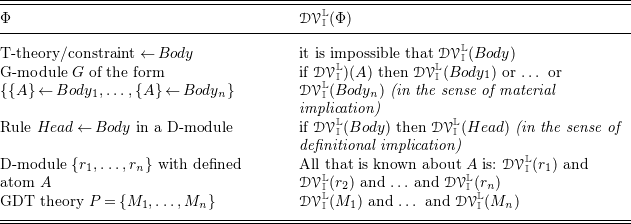
Table 9. The Denecker et al. (Reference Denecker, Lierler, Truszczyński and Vennekens2012) informal semantics for the satisfaction relation

Provided account of informal semantics of GDT theories echos the interpretation of an answer set of a basic program as a possible “interpretation” and can be seen as an informal semantics for the syntactic constructs that are fundamental in ASP practice nowadays.
6 Conclusions and Acknowledgments
In this note, we reviewed four papers and their accounts on informal semantics of logic programs under answer set semantics. We put these accounts into a uniform perspective by focusing on three components of each of the considered informal semantics, namely, (i) the interpretation of answer sets; (ii) the interpretation of syntactic expressions; and (iii) the interpretation of semantic satisfaction relation. We also discussed the relations of the presented informal semantics to two programming paradigms that emerged in the field of logic programming after the inception of the concept of a stable model: ASP and ASP-Prolog.
We would like to thank Michael Gelfond, Marc Denecker, Jorge Fandinno, Vladimir Lifschitz, Miroslaw Truszczynski, Joost Vennekens for fruitful discussions on the topic of this note. Marc Denecker brought my attention to the subject of informal semantics and his enthusiasm for the questions pertaining to this subject was contagious.
The author was partially supported by NSF 1707371.


 Open access