


1. Introduction
With the rapid development of industrialization and urbanization, the problem of air pollution has emerged, which directly affects people’s life happiness indices [Reference Pei and Shang1–Reference Haq3]. At present, air pollution monitoring methods are based mainly on ground monitoring or satellite remote sensing. Ground-based monitoring systems are installed at fixed locations, which makes it impossible to monitor the vertical distribution of pollutants, the overall pollutant concentration in the region or the trend of pollution diffusion, and the accuracy of such monitoring is strongly dependent on the number of samples and the sampling location [Reference Su, Gao, Ren, Zhang, Cao, Zhang, Chen, Liu, Ni and Liu4]. The satellite remote sensing measurement method has a long measurement cycle and high cost; coupled with the difficulty of data inversion, it is difficult to obtain the inversion law between real data and remote sensing data, and the usability of this method is low [Reference Muthukumar, Cocom, Nagrecha, Comer, Burga, Taub, Calvert, Holm and Pourhomayoun5, Reference Wang, Cai, Yang, Zhang and Du6].
An air quality monitoring system based on unmanned aerial vehicles (UAVs) as a flight platform has many advantages, such as wide monitoring level, fast data acquisition speed, and little interference from the terrain, and it can effectively compensate for the deficiencies of traditional monitoring methods [Reference Qu, Zhao, Wang, Li, Li, Xie and Zhuang7]. In the implementation of environmental detection tasks, most of the environmental detection tasks are characterized by a large three-dimensional space and the need for continuous monitoring. The use of multi-UAV to replace a single UAV in the implementation of the detection task can greatly make up for the defects of the single UAV in terms of insufficient energy, lack of resources, and a single performance and can better coordinate the task. In the atmospheric detection scenario, the purpose is to find safe paths for each UAV carrying gas measurement sensors to traverse their respective mission areas, and the acquired paths need to satisfy the maneuverability constraints of the UAVs and the synergy constraints of the mission in order to ensure the flyability of the trajectories [Reference Yang, Fan, Yu and Jia8]. The essence of this problem is to solve the problem of multiple drones detecting different task areas, and the detection path covering the entire area can provide more realistic and accurate data for the fine-grained distribution of spatial pollutants. This optimal path problem involving multiple robots cooperating to traverse all sampling points in the area of interest is usually summarized as a multi-agent coverage path planning (MCPP) problem. The problem is a subfield of trajectory planning in which the algorithm must find the optimal path for UAVs equipped with finite footprint sensors to cover the free workspace and the optimal path assignment for each UAV. The technique is applicable to inspection, precision agriculture, search and rescue, remote sensing, and other tasks [Reference Otto, Agatz, Campbell, Golden and Pesch9]. The combination of traditional task decomposition and path planning has brought many benefits to atmospheric environment monitoring. Through task decomposition, it can ensure comprehensive coverage of the monitoring area and avoid monitoring blind spots, and path planning can ensure the coverage density and distribution balance of monitoring points, ensuring the accuracy and completeness of monitoring data. Good task decomposition and path planning can enable monitoring equipment to arrive at designated monitoring points on time for real-time monitoring, reduce the impact of the monitoring process on the environment and resources, and improve the sustainability of monitoring work. In summary, reasonable task decomposition and path planning have greatly improved the efficiency, resource utilization, and data quality of monitoring work, promoting the sustainable development and intelligent application of environmental monitoring.
At present, most MCPP algorithms are developed and extended based on the existing single-drone coverage path planning (CPP) algorithms [Reference Huang, Xu, Shi, Liu and Fan10]. The common CPP algorithms include grid method and graph traversal method. The grid method divides the coverage area into grids and uses search algorithms (such as A* algorithm) to plan the path of the drone to cover all grids. The graph traversal method maps the coverage area to the graph and uses the traveling salesman problem (TSP) to solve the shortest CPP problem within that area. Davoodi proposed a heuristic approximation algorithm to find an approximate Pareto optimal solution to the problem, which used geometric objects such as Voronoi diagrams and Delaunay triangulations to solve the approximate traveler’s problem [Reference Alves, de Morais and Yamanaka11]. Rahman solved the obstacle-aware path planning problem for UAVs by using Dijkstra’s algorithm to find a detour path in the presence of an obstacle between any two sensors, minimizing the total distance traveled by all UAVs while taking into account the UAV flight time constraints [Reference Rahman, Akter and Yoon12]. Li optimized the heuristic function of A* using the ant colony algorithm (ACA) to obtain the improved A* algorithm (Imp-A*), which greatly shortens the path length of the automated rice transplanter moving between the supply pallet and the target pallet in a greenhouse nursery [Reference Li, Wang, Liu, Li and Li13]. Zheng investigated a particle swarm optimization (PSO) algorithm based on migration learning, which uses the optimal information of the historical problem to guide the particle swarm to find the optimal path quickly [Reference Zheng, Zhang and Yang14]. Zheng combined reinforcement learning with edge-assembled crossover genetic algorithms and local search heuristics to propose a reinforcement hybrid genetic algorithm for solving the well-known NP-hard TSP [Reference Zheng, Zhong, Chen and He15].
For the problem of multiple unmanned aerial vehicles (multi-UAVs) CPP, the pairing method or partitioning method can be used. The pairing method refers to specifying a drone for each target and using the CPP algorithm to plan the paths of each drone. The partitioning method refers to dividing the area into multiple subareas, assigning a drone to each subarea, and then using the CPP algorithm to plan the paths of each drone. George proposed a multi-UAV coverage area partitioning scheme for splitting convex or nonconvex regions of interest, including any number of no-fly zones, into multiple parts. This scheme improves the compactness of partitioning and compares multiple solutions based on the Hert and Lumelsky algorithms [Reference Skorobogatov, Barrado, Salamí and Pastor16]. Chen proposed an effective heuristic method for area CPP and a new multi-area allocation scheme based on minimum consumption rate based on the flight speed and scanning width of drones [Reference Chen, Zhang, Zhao, Li and He17]. This method can effectively solve the path planning problem of multiple drones covering multiple areas. Yu proposed a multi-UAV collaborative search algorithm based on greedy algorithm (MUCS-GD) and binary search algorithm (MUDS-BSAE), which further shortens the working time of multiple drones [Reference Yu and Lee18]. Ahmed proposed an autonomous landmine detection framework based on UAVs to determine coverage routes for scanning target areas [Reference Barnawi, Kumar, Kumar, Thakur, Alzahrani and Almansour19]. It extracts regions of interest using deep learning-based segmentation and then constructs coverage route plans for aerial surveys. Hong optimized a scheme for efficient autonomous execution of area coverage tasks by multiple drones [Reference Hong, Jung, Kim and Cha20]. The waypoints covering the area were assigned to each drone in the cluster, and the drones could fill a given area with their footprints in the shortest possible time without overlapping during the mission. Abdul proposed a multi-objective coverage flight path planning algorithm that enables drones to find the minimum length, collision-free, and flyable path in a three-dimensional urban environment that inhabits multiple obstacles and is used to cover spatially distributed areas [Reference Majeed and Hwang21].
After the completion of multi-UAV collaborative task planning, unmanned opportunities in the cluster execute tasks according to the predetermined task plan. However, the task environment in actual scenarios is often dynamic, and the status of drones or task points can change at any time. At this time, the drone task planning plan should also be changed accordingly. The reassignment of tasks can enable the fleet to adapt more quickly to dynamic and changing task environments, improving the responsiveness and stability of drone task planning. When performing task reassignment, consideration should be given to the category of emergency scenarios and the triggering scenarios for the reassignment, the types and quantities of tasks that need to be reassigned, as well as the current flight status and remaining energy of the drone. When the existing drones can meet the needs of task reassignment, timely task reassignment should be carried out; otherwise, additional drones should be dispatched for support or other means to solve the problem. In emergency situations, drones should first make contingency plans for task reassignment scenarios. When the fleet encounters unexpected situations during task execution, a dynamic task reassignment response mechanism will be activated based on the preset scenario.
However, there are still some challenges and problems in CPP for multiple drones, such as the efficiency and real-time performance of path planning, conflicts, and cooperation issues in collaborative work among multiple drones. When planning multiple drone paths, it is necessary to comprehensively consider task complexity, communication load, computing resources, and real-time factors. When planning multiple drone coverage paths, it is necessary to consider the size of the coverage area, the number of drones, and the type of target task requires selecting appropriate planning methods. Therefore, to address the current problems of multi-UAV in environmental detection, this paper proposes a multi-UAV collaborative environmental detection mission planning system, which mainly contains the following parts:
-
A multi-UAV collaborative mission planning method for irregular three-dimensional spaces is proposed, which can quickly partition, sample, and plan coverage detection paths for multiple drones in irregular three-dimensional spaces. Nonuniform rational B-spline (NURBS) curves are used to smooth the planned paths to meet the requirements of continuous flight of drones, thereby reducing unnecessary energy consumption of drones and improving task execution efficiency. The problem of traditional multi-drone communication cooperation and individual conflicts has been solved with the help of a robot operating system (ROS), and the feasibility and stability of this method have been verified under Linux system with the help of multi-drone ground control stations and Gazebo simulation platform.
-
Simulated annealing-whale optimization algorithm (SA-WOA) is proposed to address the problems of slow convergence speed, poor path search ability, susceptibility to local optima, and unsatisfactory planned path length in traditional CPP algorithms. It introduces SA mechanism, nonlinear convergence factor, and adaptive weight in the contraction and encirclement stage of WOA and introduces Levy flight mechanism to perturb the old solution in the search and foraging stage. Then, it improves the metropolis criterion in SA and introduces adaptive warming mechanism to improve the optimization speed of the algorithm so that SA-WOA can plan the coverage detection path of multiple drones faster and better. Finally, using the eil76 and st70 datasets, SA-WOA was compared with other path planning algorithms, and the results showed that the proposed SA-WOA had faster convergence speed and better convergence results.
-
The hardware platform of the multi-computer collaborative environmental detection system is designed and constructed, and environmental gas measurement experiments are carried out. Under the premise that 1-week continuous gas measurement shows the consistency and accuracy of the multiple sets of gas measurement devices formed in this paper, the multi-UAV detection paths are generated with the help of multi-UAV collaborative task planning method to cover the target space for detection, and the pollutant distribution of the space is constructed with the help of the kriging interpolation method, which verifies that the multi-UAV collaborative environmental detection system designed in this paper has the feasibility and effectiveness. It can help staff to have a deep understanding of the distribution of pollutants within the three-dimensional space range and formulate corresponding countermeasures, which has high application value in three-dimensional space atmospheric environment quality measurement, spatial distribution analysis of atmospheric pollutants, traceability, and other aspects.
In summary, this paper designs a multi-UAV cooperative mission planning system for atmospheric environment detection scenarios. Section 2 briefly models the problem of collaborative multicomputer multi-UAV environmental detection. Section 3 adopts the synergistic method of from-and-to equilibrium division by swarm and convex decomposition of concave points for fast division of spatial regions, and an SA-WOA based on the adaptive weight and SA strategy is proposed. In Section 4, simulation scenarios are designed to test the multi-UAV cooperative mission planning system, which verifies that the multi-UAV cooperative mission planning system designed in this paper is able to quickly formulate reasonable multi-UAV detection paths while meeting the flight constraints of the aircraft fleet. In Section 5, a hardware system platform is designed and built for multi-UAV environmental detection task planning, followed by environmental gas measurement experiments. Section 6 contains conclusions and suggestions for future work.
2. Problem modeling
In the rotorcraft atmospheric environment detection application, to ensure that the detection results can truly and completely reflect the fine-grained distribution of atmospheric pollutants in the detection space, the sampling points must be uniformly spread throughout the entire three-dimensional space, and each UAV must carry a gas sensing device for traversing all the sampling points in the space; multi-UAVs can cooperate with each other to ensure that higher operational efficiency is obtained in real time.
To address this problem, the basic idea for collaborative multi-UAV spatial exploration in this paper is to divide the three-dimensional space into multiple task subareas, assign them to UAV clusters, and transform the multi-UAV path planning problem into a single-UAV path planning problem with the solution shown in Fig. 1.
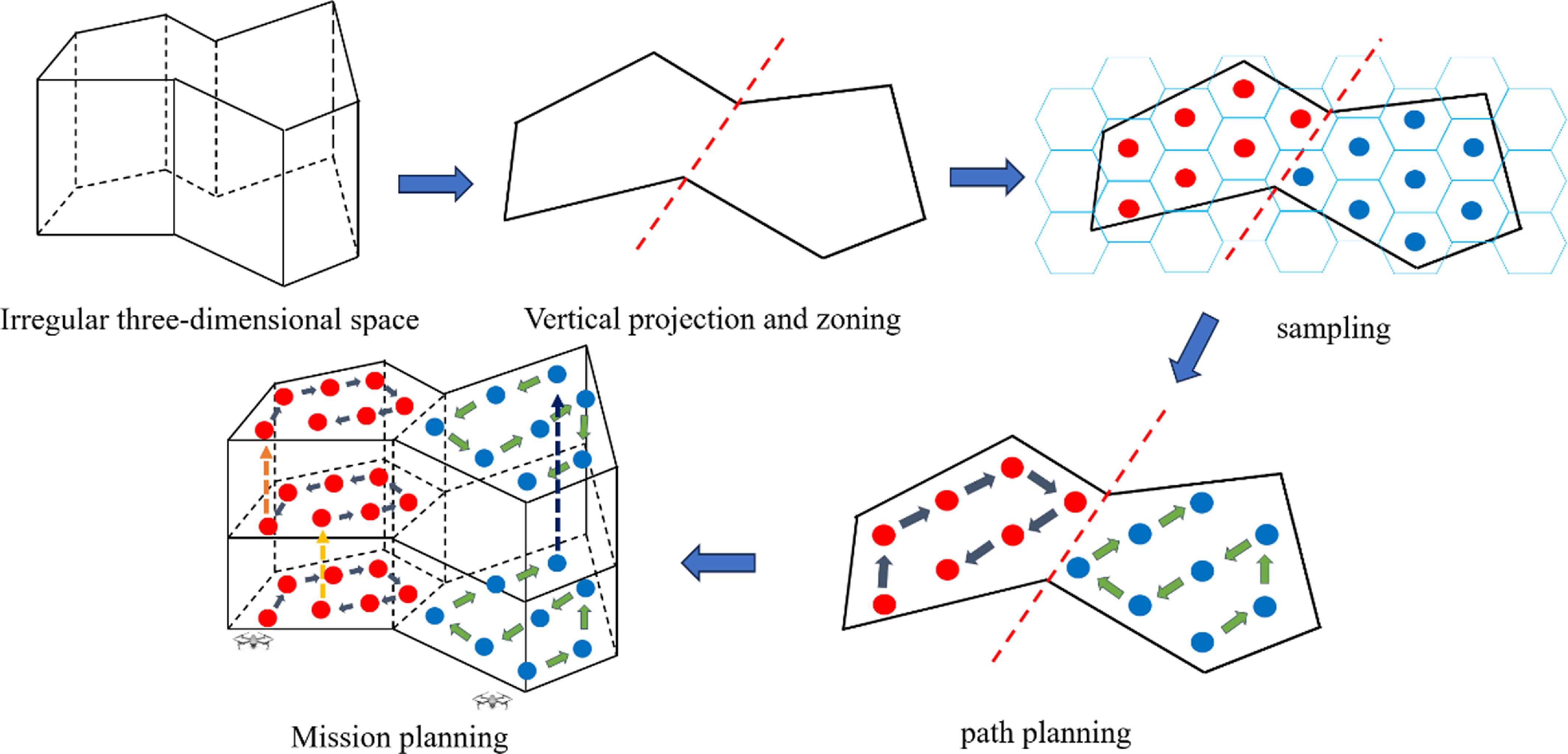
Figure 1. Modeling of the multi-UAV cooperative space exploration problem.
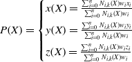
As shown in Fig. 1, the detection space is first vertically projected to obtain a planar irregular region, which is roughly divided into a convex region and a concave region in terms of shape, and the regions are quickly divided into multiple task subregions with balanced areas. Each task subregion is covered using a square hexagon, with the center of the hexagon as the UAV sampling point, resulting in a collection of sampling points for each task subregion. Then, the improved SA-WOA is used to perform path planning for the set of sampling points in each task subregion separately to obtain the shortest task path traversing all the sampling points, which is rounded using the NURBS curve. After obtaining the feasible detection paths for each UAV to detect the corresponding mission subspace, the paths are combined to obtain the overall mission detection scheme for coordinated multi-UAV space detection.
3. Design of a multi-UAV cooperative mission planning system
3.1. Irregular region division
A well-balanced division of the vertical projection plane region of space is a prerequisite for fast multi-UAV detection missions, but researchers often have different understandings of the metrics for well-balanced division. In this paper, the equal area of subregions is used as the basis for the equalization of regions, and the convex regions are equalized according to the direction of UAV swarms; for the concave regions, a combination of concave-point removal and concave-convex decomposition is chosen for the division.
The vertical projection of the probe space is assumed to be a convex polygonal region, as shown in Fig. 2, which can be denoted as
 $P=\{P_{i}|i=1,2,\ldots,N\}$
; the task region is assigned to the swarm of UAVs, which is represented as
$P=\{P_{i}|i=1,2,\ldots,N\}$
; the task region is assigned to the swarm of UAVs, which is represented as
 $U=\{U_{i}|i=1,2,\ldots,n\}$
; and the algorithmic flow for the balanced partitioning of the region in accordance with the incoming direction of the UAVs is shown in Table I. The effect of the partitioning is shown in Fig. 2.
$U=\{U_{i}|i=1,2,\ldots,n\}$
; and the algorithmic flow for the balanced partitioning of the region in accordance with the incoming direction of the UAVs is shown in Table I. The effect of the partitioning is shown in Fig. 2.
Table I. The convex zoning process.
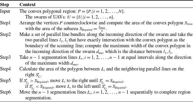
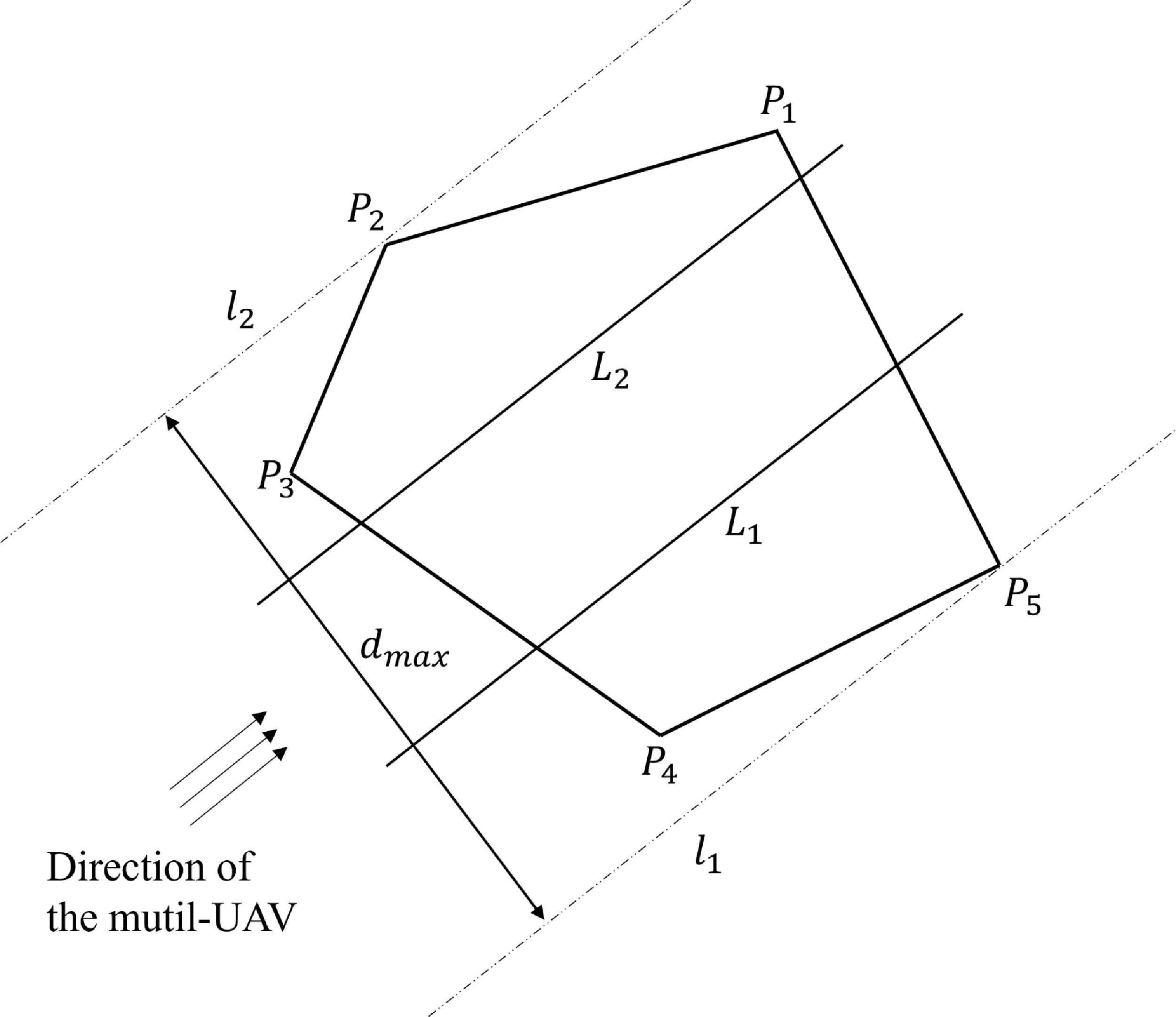
Figure 2. The convex polygonal regions equalized by swarms of UAVs.
Concave-point removal is a relatively traditional concave-point localization algorithm in which the vertices of the concave polygon are traversed to determine all the concave points and the vertices on both sides of the concave point are directly connected to remove the concave points. As shown in Fig. 3(a), by traversing all the vertices to determine that
 $B$
is concave, directly connecting the vertices
$B$
is concave, directly connecting the vertices
 $A$
and
$A$
and
 $C$
at the two ends of
$C$
at the two ends of
 $B$
and deleting the edges
$B$
and deleting the edges
 $AB$
and
$AB$
and
 $BC$
, a new region
$BC$
, a new region
 $\textit{ACEFG}$
is obtained as a convex polygon.
$\textit{ACEFG}$
is obtained as a convex polygon.
The traditional notch convex decomposition method defines the boundary extension line of the notch close to the polygon boundary as boundary 1 and the other extension line as boundary 2. When the partition area on the outside of boundary 1 is smaller than the required area, the partition line is rotated from boundary 1 to boundary 2 on the notch axis until the partition area is equal to the required area; then, the subregion is divided, and the division of the remaining area continues.
In addition, we consider two special cases to improve the traditional notch convex decomposition method, as shown in Fig. 3(b). In the first case, the area outside boundary 1 is larger than the required area, the partition line is located on the outside of boundary 1, and the planning of the remaining area continues; the notch still exists so the notch continues to be divided using the method described above. In the second case, the partition line coincides with boundary 2 and still does not reach the required area; then, the partition line is translated in the direction perpendicular to boundary 2 until the required subarea is divided.
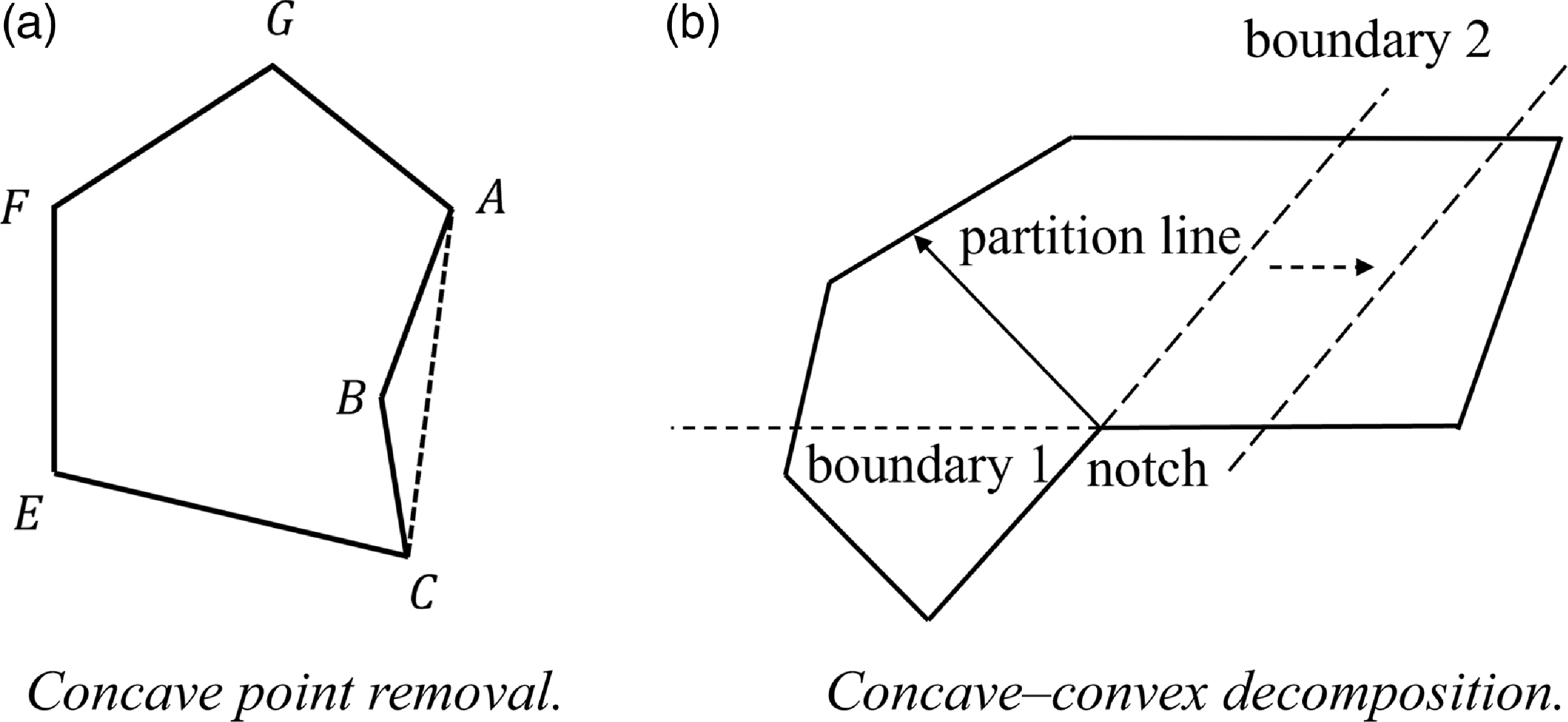
Figure 3. A diagram of the methods used to divide the concave area.
The concave point removal method shown in Fig. 3(a) can transform a problem with concave regions into the problem of dividing the convex regions, but if the excess task region
 $ABC$
generated is too large, the path and energy consumption of the UAV increase. Directly using the concave point convex decomposition method in Fig. 3(b) will divide all the concave points in the region one by one, which will produce too many fragmented task regions; additionally, the divided subregions are not regular and cannot be allocated to the whole fleet well.
$ABC$
generated is too large, the path and energy consumption of the UAV increase. Directly using the concave point convex decomposition method in Fig. 3(b) will divide all the concave points in the region one by one, which will produce too many fragmented task regions; additionally, the divided subregions are not regular and cannot be allocated to the whole fleet well.
Therefore, in this paper, we consider treating concave regions by removing some of the concave points and then convexly decomposing the remaining concave points, thus dividing the concave region into a combination of one or more convex polygonal regions. First, we traverse all the concave points in the whole region and set the parameter
 $\delta$
to express the cost of removing the concave point as follows:
$\delta$
to express the cost of removing the concave point as follows:
 \begin{equation}\delta =\frac{S_{\textit{increase}}}{S_{Area}}\end{equation}
where
 $S_{\textit{increase}}$
denotes the increased task area after removing the dents and
$S_{\textit{increase}}$
denotes the increased task area after removing the dents and
 $S_{Area}$
denotes the original task area before removing the dents. A threshold denoted as
$S_{Area}$
denotes the original task area before removing the dents. A threshold denoted as
 $w\;\alpha$
is set, and if
$w\;\alpha$
is set, and if
 $\rho \lt \alpha$
is satisfied, then the above method is directly used to remove the dimple; otherwise, the dimple removal method is abandoned. As shown in Fig. 4(b), some concave points are directly removed after meeting the threshold condition, leaving only a few concave points; at this time, the task area is relatively regular and easy to divide, and the remaining concave points use the method of convex decomposition of concave points, as shown in Fig. 4(c).
$\rho \lt \alpha$
is satisfied, then the above method is directly used to remove the dimple; otherwise, the dimple removal method is abandoned. As shown in Fig. 4(b), some concave points are directly removed after meeting the threshold condition, leaving only a few concave points; at this time, the task area is relatively regular and easy to divide, and the remaining concave points use the method of convex decomposition of concave points, as shown in Fig. 4(c).
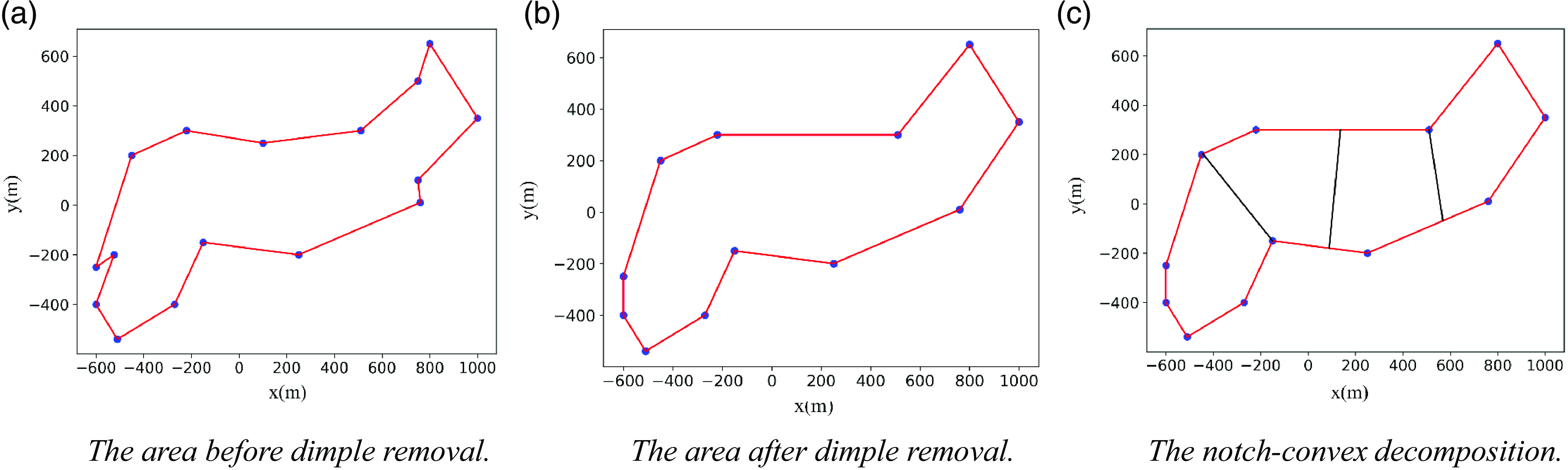
Figure 4. The concave area division effect.
3.2. Detection area sampling
In plane geometry, the three possible geometric shapes that can cover a region completely and without overlap in a polygon with vertices equidistant from the geometric center are the regular triangle, the square, and the regular hexagon. A regular hexagon has the largest area provided that the radii of the outer circles are equal, so the entire geographic area can be covered by the smallest number of regular hexagons. The effective measurement area for UAV single-point hover sampling is assumed to be spherical, and the use of a positive hexagonal fill in the spatial projection area ensures that both the number of sampling points and the area of sampling overlap are relatively small, as shown in Fig. 5.
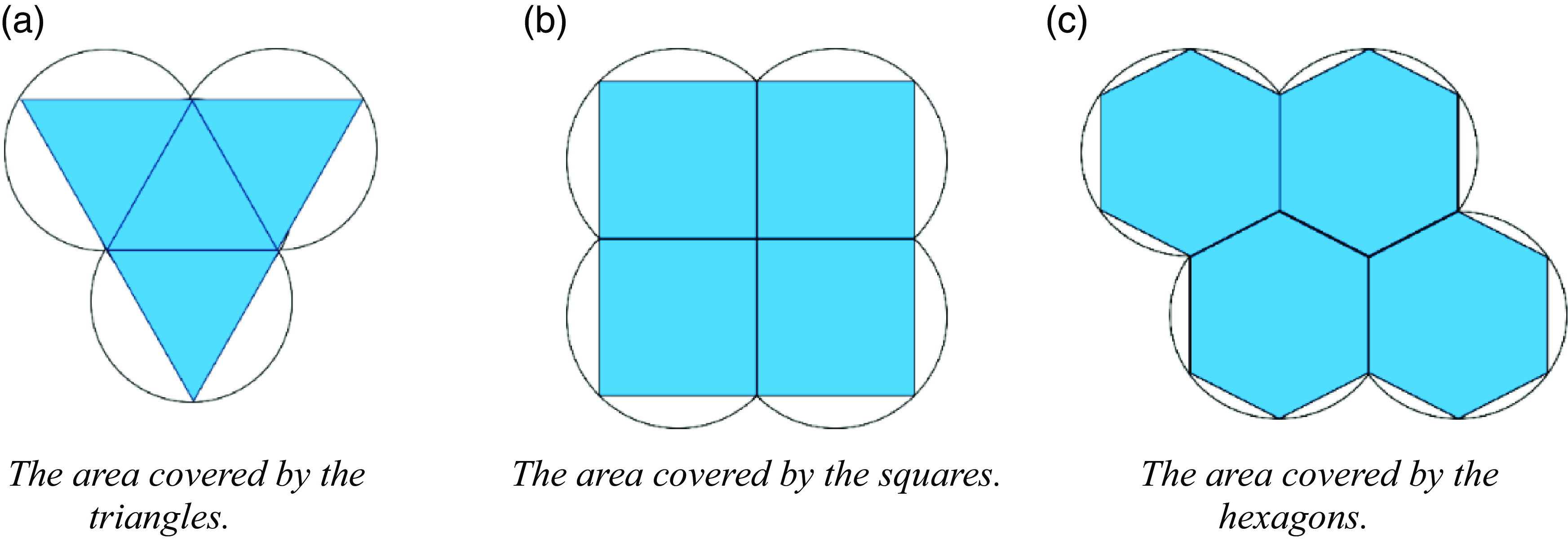
Figure 5. The graphics overlay comparison.
The measurement area is assumed to be an irregular three-dimensional space with a height of
 $H$
. The effective measurement range of UAV single-point hover sampling is abstracted as a hexagonal prism with a side length of
$H$
. The effective measurement range of UAV single-point hover sampling is abstracted as a hexagonal prism with a side length of
 $L$
and a height of
$L$
and a height of
 $\sqrt{3}L$
in Fig. 6(a), and the UAV sampling point is located in the center of the hexagonal prism; this ensures that the UAVs fly to adjacent sampling points in the vertical or horizontal directions with path lengths of
$\sqrt{3}L$
in Fig. 6(a), and the UAV sampling point is located in the center of the hexagonal prism; this ensures that the UAVs fly to adjacent sampling points in the vertical or horizontal directions with path lengths of
 $\sqrt{3}L$
, which is more conducive to the calculation of path lengths. The hexagonal prism sampling units are used to fill the entire irregular three-dimensional space, and the three-dimensional space is then divided into N layers of different heights, each containing the same number of sampling units, to sample the irregular three-dimensional space, as shown in Fig. 6(b).
$\sqrt{3}L$
, which is more conducive to the calculation of path lengths. The hexagonal prism sampling units are used to fill the entire irregular three-dimensional space, and the three-dimensional space is then divided into N layers of different heights, each containing the same number of sampling units, to sample the irregular three-dimensional space, as shown in Fig. 6(b).
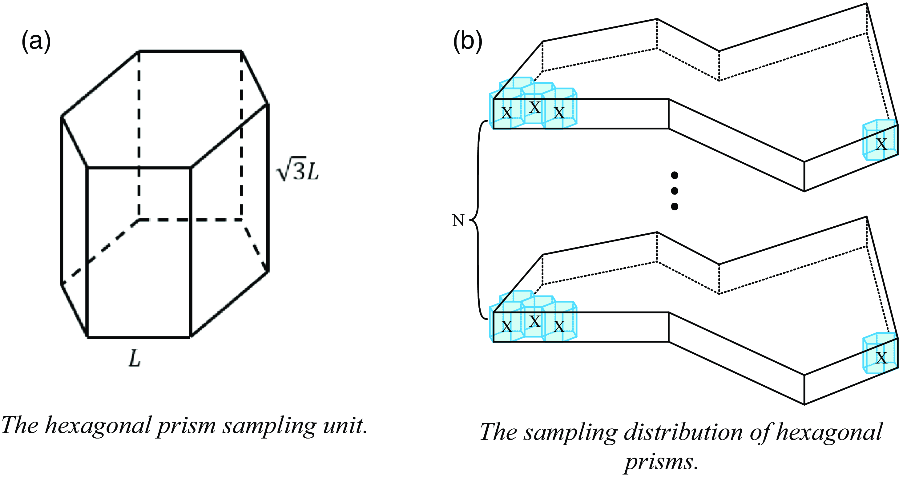
Figure 6. The stereo space sampling.
The fleet has a total of
 $n$
UAVs, all of which are spatially probed using layered measurements, with the number of layers set to
$n$
UAVs, all of which are spatially probed using layered measurements, with the number of layers set to
 $N=\frac{H}{\sqrt{3}L}$
and the number of sampling points for the
$N=\frac{H}{\sqrt{3}L}$
and the number of sampling points for the
 $i$
th UAV hovering at each layer set to
$i$
th UAV hovering at each layer set to
 $m_{i}$
; then, the path length is expressed as follows:
$m_{i}$
; then, the path length is expressed as follows:
 \begin{equation}s=(m_{i}-1)*\sqrt{3}L*N+\sqrt{3}L*(N-1)\end{equation}
The value of
 $L$
during the sampling process directly affects the coverage density of spatial sampling. If value of
$L$
during the sampling process directly affects the coverage density of spatial sampling. If value of
 $L$
is too small, UAVs may not be able to complete the assigned task due to too many sampling points. If value of
$L$
is too small, UAVs may not be able to complete the assigned task due to too many sampling points. If value of
 $L$
is too large, it will lead to sparse distribution of sampling points, and UAVes may not be able to accurately obtain the distribution of pollutants in that space. Therefore, it is necessary to find the optimal value of
$L$
is too large, it will lead to sparse distribution of sampling points, and UAVes may not be able to accurately obtain the distribution of pollutants in that space. Therefore, it is necessary to find the optimal value of
 $L$
that can meet the energy constraints of drones. According to the task subspace parameters after the area division is completed, the space decomposition method based on the six prism is used first to uniformly decompose each task subspace area to obtain a certain number of sampling points, and then the sampling points as flight waypoints are used. According to formula (2), we can directly evaluate the approximate energy consumption of each UAV under the current value of
$L$
that can meet the energy constraints of drones. According to the task subspace parameters after the area division is completed, the space decomposition method based on the six prism is used first to uniformly decompose each task subspace area to obtain a certain number of sampling points, and then the sampling points as flight waypoints are used. According to formula (2), we can directly evaluate the approximate energy consumption of each UAV under the current value of
 $L$
, compare it with the maximum energy of the UAV, and then adjust the size of
$L$
, compare it with the maximum energy of the UAV, and then adjust the size of
 $L$
. If the maximum energy carried by the drone is less than the energy required for the current planned path, the size of the hexagonal prism decomposition unit is adjusted to decompose again until the energy meets the demand. Finally, the value of
$L$
. If the maximum energy carried by the drone is less than the energy required for the current planned path, the size of the hexagonal prism decomposition unit is adjusted to decompose again until the energy meets the demand. Finally, the value of
 $L$
is determined, and this value is used to construct a hexagonal prism sampling unit to sample each subspace to obtain the optimal set of sampling points for the target space detected by the aircraft group.
$L$
is determined, and this value is used to construct a hexagonal prism sampling unit to sample each subspace to obtain the optimal set of sampling points for the target space detected by the aircraft group.
3.3. Improved SA-WOA path planning algorithm
The WOA is a new bionic intelligent optimization algorithm that simulates the foraging behavior of humpback whales and has the advantages of a simple structure and few adjustment parameters. In the WOA, the optimal position in the current group is assumed to be the prey, and all the other whale individuals in the group surround the optimal individual; their positions are updated according to the optimization rule until the end condition is satisfied. The entire whale foraging process can be divided into three phases: encircling prey, foaming attacks, and random searches [Reference Si and Li22].
The SA algorithm is a commonly used algorithm in UAV path planning research. It is a global search optimization algorithm designed to simulate the annealing process in physics, where a higher temperature is set in the initial state and the current solution is changed to produce a new solution during each cooling process. The difference between the new solution and the previous solution is calculated, and the decision of whether to accept the new solution is made with a certain probability; repetitive iterations of these steps are applied until the temperature is the lowest, which produces the optimal solution [Reference Hemici, Zouache, Brahmi, Got and Drias23].
The traditional whale optimization algorithm has few adjustable parameters and a simple structure, but it cannot adjust the convergence speed, is prone to problems such as premature convergence, and easily falls into local extremes for multipeak functions, which leads to the inability of the algorithm to obtain the global optimum [Reference Xu, Zhao, Li, Hu and Hou24]. However, the mechanism of accepting new solutions with a certain probability in the SA algorithm can be a good solution to the problem of multipeak functions falling into local extrema [Reference Long, Liu, Qiu, Li, Guo, Shi and AbouOmar25]. Therefore, to plan the optimal detection path of multiple UAVs more quickly and with better results, this paper improves upon the WOA based on the SA algorithm; the flow chart of the improved algorithm is shown in Fig. 7.
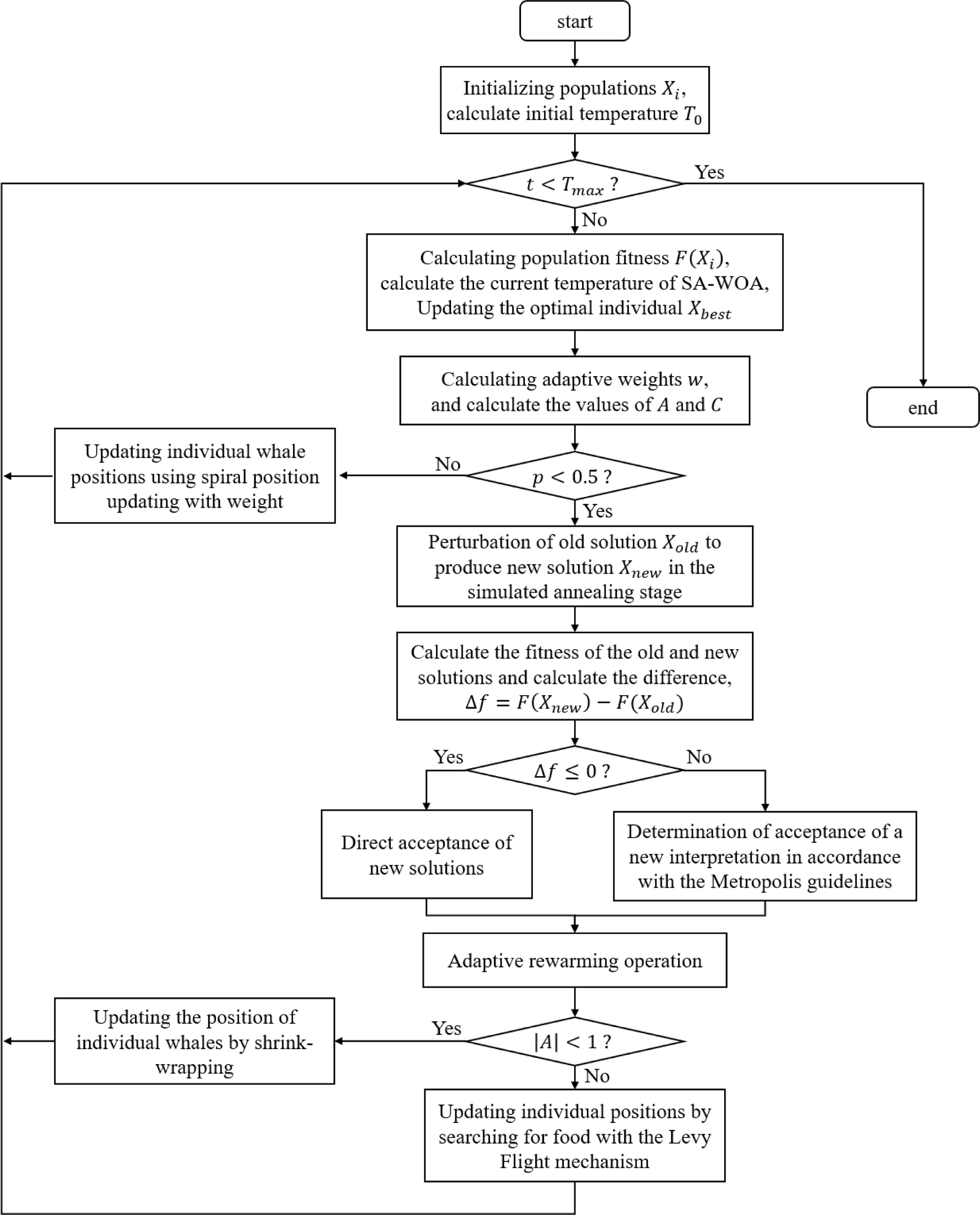
Figure 7. The SA-WOA algorithmic framework.
In Fig. 7,
 $X_{i}$
denotes the population at the very beginning of the algorithm,
$X_{i}$
denotes the population at the very beginning of the algorithm,
 $F(X_{i})$
denotes its fitness,
$F(X_{i})$
denotes its fitness,
 $T_{0}$
denotes the initial temperature of the algorithm,
$T_{0}$
denotes the initial temperature of the algorithm,
 $t$
represents the current number of iterations,
$t$
represents the current number of iterations,
 $T_{max}$
denotes the maximum number of iterations set, and
$T_{max}$
denotes the maximum number of iterations set, and
 $A$
and
$A$
and
 $C$
are the coefficients that the whale population in the algorithm relies on when it performs the contraction envelopment. Since individual whales must contract their encirclement while swimming spirally toward their prey, in order to clearly express this behavior, a parameter
$C$
are the coefficients that the whale population in the algorithm relies on when it performs the contraction envelopment. Since individual whales must contract their encirclement while swimming spirally toward their prey, in order to clearly express this behavior, a parameter
 $p$
is set here to determine whether the current iteration uses spiral position updating or contraction encirclement to update the position of individual whales.
$p$
is set here to determine whether the current iteration uses spiral position updating or contraction encirclement to update the position of individual whales.
The SA-WOA algorithm first calculates the initialized population and computes the initial temperature
 $T_{0}$
, sets the maximum number of iterations
$T_{0}$
, sets the maximum number of iterations
 $T_{max}$
, computes the population fitness, the value of the adaptive weighting factor and the values of
$T_{max}$
, computes the population fitness, the value of the adaptive weighting factor and the values of
 $A$
and
$A$
and
 $C$
during each iteration, and then generates a random number
$C$
during each iteration, and then generates a random number
 $p$
. When the value of
$p$
. When the value of
 $p$
is not less than 0.5, the algorithm chooses the spiral position updating method with weights. Otherwise, it enters the SA stage, which first perturbs the current solution to a certain extent to generate a new solution, and then calculates the difference
$p$
is not less than 0.5, the algorithm chooses the spiral position updating method with weights. Otherwise, it enters the SA stage, which first perturbs the current solution to a certain extent to generate a new solution, and then calculates the difference
 ${f}$
between the current solution and the new solution’s fitness; when
${f}$
between the current solution and the new solution’s fitness; when
 ${f\leq 0}$
, it indicates that the generated new solution is better than the old one, and the new solution should be accepted directly at this time, or else it indicates that the new solution is worse than the current one. In order to avoid the algorithm falling into local optimality and improve its ability to seek the optimal solution, the new solution should be accepted according to the metropolis criterion. When the SA stage of the current solution is updated, the temperature of the current iteration is calculated with the help of the adaptive tempering function. And then judge the current iteration A take value; when
${f\leq 0}$
, it indicates that the generated new solution is better than the old one, and the new solution should be accepted directly at this time, or else it indicates that the new solution is worse than the current one. In order to avoid the algorithm falling into local optimality and improve its ability to seek the optimal solution, the new solution should be accepted according to the metropolis criterion. When the SA stage of the current solution is updated, the temperature of the current iteration is calculated with the help of the adaptive tempering function. And then judge the current iteration A take value; when
 $| A| \lt 1$
, the algorithm chooses the shrink-wrap strategy; at this time, the whale will converge toward the global optimal solution, gradually narrowing the search range during the search process, which helps to improve the convergence speed and stability of the algorithm, or else with the help of the Levy flight mechanism to carry out a random search foraging, at this time the whale will carry out a random search throughout the entire search space, which helps to maintain the diversity of the algorithm and avoid falling into local optimal solutions. After the iterative process is completed, the optimal population and its fitness are obtained, which corresponds to the optimal traversal order of the sampling points and their corresponding path lengths in the path planning problem.
$| A| \lt 1$
, the algorithm chooses the shrink-wrap strategy; at this time, the whale will converge toward the global optimal solution, gradually narrowing the search range during the search process, which helps to improve the convergence speed and stability of the algorithm, or else with the help of the Levy flight mechanism to carry out a random search foraging, at this time the whale will carry out a random search throughout the entire search space, which helps to maintain the diversity of the algorithm and avoid falling into local optimal solutions. After the iterative process is completed, the optimal population and its fitness are obtained, which corresponds to the optimal traversal order of the sampling points and their corresponding path lengths in the path planning problem.
3.1.1 Adaptive weighting improvement
The weight factor is the key factor to balance the global exploration ability and local optimization ability of the algorithm, because the whale optimization algorithm is updated differently from the particle swarm algorithm, the whale optimization algorithm is updated on the basis of the position of the optimal whale when updating, and the adaptive weights are added to the head whale instead of the step size as in the case of the particle swarm algorithm, the value of the weights is adjusted so that the closer the position of the optimal position is, the smaller the perturbation to the head whale [Reference Liu, Yang, Li and Zhang26].
The adaptive weighting factor
 $w$
is introduced into the foaming attack phase of the whale optimization algorithm. The humpback whale initiates its attack by using contraction encirclement and spiral encirclement, which occur simultaneously; thus, the probability of the whale choosing each strategy is assumed to be
$w$
is introduced into the foaming attack phase of the whale optimization algorithm. The humpback whale initiates its attack by using contraction encirclement and spiral encirclement, which occur simultaneously; thus, the probability of the whale choosing each strategy is assumed to be
 $0.5$
in the algorithm, and this process is represented by the following mathematical expression:
$0.5$
in the algorithm, and this process is represented by the following mathematical expression:
 \begin{equation}X\left(t+1\right)=w*X^{*}\left(t\right)-A*D\end{equation}
 \begin{equation}X(t+1)=D'*e^{bl}*cos2\pi l+w*X^{*}(t)\end{equation}
where
 $t$
is the current number of iterations,
$t$
is the current number of iterations,
 $X^{*}(t)$
is the currently acquired prey position vector,
$X^{*}(t)$
is the currently acquired prey position vector,
 $X(t+1)$
is the next position vector of the whale,
$X(t+1)$
is the next position vector of the whale,
 $D'$
is the distance between the individual and the current optimal position,
$D'$
is the distance between the individual and the current optimal position,
 $b$
is a logarithmic helical shape constant taken as 1,
$b$
is a logarithmic helical shape constant taken as 1,
 $l$
is a random number in
$l$
is a random number in
 $[\!-\!1,1]$
, and
$[\!-\!1,1]$
, and
 $D$
is the position update vector of the encircling prey phase, which is defined as follows:
$D$
is the position update vector of the encircling prey phase, which is defined as follows:
 \begin{equation}D=|C*X^{*}\left(t\right)-X\left(t\right)|\end{equation}
In formula (3) and formula (5),
 $A$
and
$A$
and
 $C$
are coefficient vectors, which are defined by the following equations:
$C$
are coefficient vectors, which are defined by the following equations:
 \begin{equation}A=2a*r_{1}-a\end{equation}
 \begin{equation}C=2*r_{2}\end{equation}
where
 $a$
is the convergence factor, which decreases linearly from 2 to 0 with the number of iterations;
$a$
is the convergence factor, which decreases linearly from 2 to 0 with the number of iterations;
 $r_{1}$
and
$r_{1}$
and
 $r_{2}$
are random numbers in
$r_{2}$
are random numbers in
 $[0,1]$
.
$[0,1]$
.
 $w$
is the improved adaptive weight, which is generated as shown below, where the adaptations of the individual whales are sorted in ascending order during the iterative process:
$w$
is the improved adaptive weight, which is generated as shown below, where the adaptations of the individual whales are sorted in ascending order during the iterative process:
 \begin{equation}F=\left\{f_{i}|i=1,2,3,4,5\ldots,N\right\}\end{equation}
Then,
 $F$
is divided into two parts to find the left and right average adaptations, denoted as
$F$
is divided into two parts to find the left and right average adaptations, denoted as
 $f_{avg1}$
and
$f_{avg1}$
and
 $f_{avg2}$
, respectively, where
$f_{avg2}$
, respectively, where
 $f_{avg1}$
<
$f_{avg1}$
<
 $f_{avg2}$
.
$f_{avg2}$
.
 \begin{equation}f_{avg1}=\frac{\sum _{i=1}^{i=N/2}f_{i}}{N/2},f_{avg2}=\frac{\sum _{i=\frac{N}{2}+1}^{i=N}f_{i}}{N/2}\end{equation}
where the fitness of the current individual whale, denoted as
 $f_{t}$
, is compared to
$f_{t}$
, is compared to
 $f_{avg1}$
and
$f_{avg1}$
and
 $f_{avg2}$
to categorize the weights as follows:
$f_{avg2}$
to categorize the weights as follows:
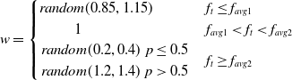 \begin{equation}w=\begin{cases} \textit{random}(0.85,1.15) & f_{t}\leq f_{avg1}\\ \;\;\;\;\;\;\;\;\;\;\;\;1 & f_{avg1}\lt f_{t}\lt f_{avg2}\\ \begin{array}{cc} \textit{random}(0.2,0.4) & p\leq 0.5\\ \textit{random}(1.2,1.4) & p\gt 0.5 \end{array} & f_{t}\geq f_{avg2} \end{cases}\end{equation}
If
 $f_{t}\leq f_{avg1}$
, the fitness of the current whale individual is better than the average fitness of the better group, which indicates that the individual has a dominant position in the population. At this time, the optimal whale individual has a small range of jitter, which is conducive to exploring the local optimum values, so
$f_{t}\leq f_{avg1}$
, the fitness of the current whale individual is better than the average fitness of the better group, which indicates that the individual has a dominant position in the population. At this time, the optimal whale individual has a small range of jitter, which is conducive to exploring the local optimum values, so
 $w$
should be defined as a random number in
$w$
should be defined as a random number in
 $(0.85,1.15)$
.
$(0.85,1.15)$
.
If
 $f_{t}\geq f_{avg2}$
, the fitness of the current individual whale is worse than the average fitness of the worse group, which indicates that the position of this individual is not ideal. At this time, to broaden the global exploration,
$f_{t}\geq f_{avg2}$
, the fitness of the current individual whale is worse than the average fitness of the worse group, which indicates that the position of this individual is not ideal. At this time, to broaden the global exploration,
 $w$
should be defined as a random number in
$w$
should be defined as a random number in
 $(0.2,0.4)$
or
$(0.2,0.4)$
or
 $(1.2,1.4)$
with a probability of
$(1.2,1.4)$
with a probability of
 $50\%$
, which is beneficial for the individual in searching for prey in other positions and enhances the global exploration ability.
$50\%$
, which is beneficial for the individual in searching for prey in other positions and enhances the global exploration ability.
In other cases, the current individual whale is in a general position in the group, in which case
 $w$
is set to 1, as this is sufficient to let the whale approach the optimal position according to the logic of the original algorithm.
$w$
is set to 1, as this is sufficient to let the whale approach the optimal position according to the logic of the original algorithm.
This random inertia weighting strategy is adopted so that the weights no longer take a fixed value but are randomly adjusted according to fitness, which makes the whales more diversified in the process of searching for prey, improves the algorithm’s solution accuracy and convergence speed, and decreases the likelihood of missing the global optimal solution.
3.3.2 Randomized search strategy
In the random search prey phase, the new solution is generated by perturbing the old solution to a certain extent. At this time, the new solution should satisfy two conditions: one is that the change between the old and new solutions cannot lead to too large change in the objective function, and the other is that the new solution should spread across the solution space to improve the algorithm’s chances of finding the globally optimal solution. In the traditional whale optimization algorithm, the update mechanism drives the individuals in the population to move toward the optimal individual in the current iteration without considering the position of the center of the population or the positions of the individuals in the previous generation, and this prevents the whale population from adequately covering the entire search space. Therefore, the algorithm is prone to falling into a locally optimal solution, and premature convergence occurs. Therefore, in this paper, the Levy flight mechanism is introduced to perturb the old solution in updating the position.
The Levy flight is a random wandering process and is a good search strategy [Reference Xu, Zhang and Zhang27]; the new generation of optimal individuals generated by Levy flight perturbation is calculated as follows:
 \begin{equation}X_{best}\left(t+1\right)=X_{best}\left(t\right)+\textit{s}\,\ast\,{Levy}(\beta )\end{equation}
where
 $X_{best}(t)$
denotes the optimal individual produced by the previous
$X_{best}(t)$
denotes the optimal individual produced by the previous
 $t$
iterations,
$t$
iterations,
 $s$
denotes the Levy search path, and
$s$
denotes the Levy search path, and
 $Levy(\beta )$
denotes the stochastic search path with the following expression:
$Levy(\beta )$
denotes the stochastic search path with the following expression:
 \begin{equation}Levy\left(\beta \right)\sim \frac{\mu }{|v|^{\frac{1}{\beta }}}\end{equation}
where the value of
 $\beta$
is generally in the range of
$\beta$
is generally in the range of
 $1\lt \beta \lt 3$
; here, we take
$1\lt \beta \lt 3$
; here, we take
 $\beta =1.5$
, and
$\beta =1.5$
, and
 $\mu$
and
$\mu$
and
 $v$
obey the normal distribution as follows:
$v$
obey the normal distribution as follows:
 \begin{equation}\mu \sim N\left(0,\sigma ^{2}\right);\; v\sim N(0,1)\end{equation}
 \begin{equation}\sigma =\left[\frac{{{\Gamma}} \left(1+\beta \right)*\sin (\pi *\frac{\beta }{2})}{\beta *{{\Gamma}} \left(\frac{1+\beta }{2}\right)\mathrm{*}2^{\frac{\beta -1}{2}}}\right]^{\frac{1}{\beta }}\end{equation}
where
 ${{\Gamma}}$
is the Gamma function.
${{\Gamma}}$
is the Gamma function.
3.3.3 Metropolis guidelines improvement
In the SA algorithm, the metropolis criterion determines whether to accept a new solution, which indirectly determines the algorithm’s optimization ability and convergence speed. The metropolis criterion expression for the traditional SA algorithm is
 \begin{equation}p=e^{-\frac{E\left(X_{new}\right)-E(X_{old})}{T}}\end{equation}
However, for path planning problems of different sizes, the value of
 $E(X_{new})-E(X_{old})$
may greatly differ from the current value of
$E(X_{new})-E(X_{old})$
may greatly differ from the current value of
 $T$
, which leads to the value of
$T$
, which leads to the value of
 $p$
being too large or too small, thus affecting the convergence speed of the algorithm. In this paper, the criterion has been improved to avoid this discrepancy:
$p$
being too large or too small, thus affecting the convergence speed of the algorithm. In this paper, the criterion has been improved to avoid this discrepancy:
 \begin{equation}p=e^{-\frac{|f\left(new\right)-f(old)|}{AT}}, A=L_{\textit{Initial}}\end{equation}
where
 $f(new)$
represents the fitness function of the new solution, which is defined here as the total length of the path of the new solution,
$f(new)$
represents the fitness function of the new solution, which is defined here as the total length of the path of the new solution,
 $T$
is the current temperature, and the new parameter
$T$
is the current temperature, and the new parameter
 $A$
represents the length of the shortest path among the nearest-neighbor paths. There are
$A$
represents the length of the shortest path among the nearest-neighbor paths. There are
 $N$
such paths to represent the scale of the solution of the problem so that the value of
$N$
such paths to represent the scale of the solution of the problem so that the value of
 $p$
can be stabilized within a certain range to ensure that the algorithm converges as soon as possible.
$p$
can be stabilized within a certain range to ensure that the algorithm converges as soon as possible.
3.3.4 Adaptive warming mechanism
Most of the traditional SA algorithms set the initial temperature high enough to allow the algorithm to achieve better global optimization, but there is no fixed way to set the temperature. If the initial temperature is not set properly, the algorithm will likely converge slowly, and it will not be easy to find the optimal solution. To adapt the initial temperature to the size of this path planning problem, in this paper, the initial temperature is set to the variance of the nearest-neighbor path lengths, of which there are
 $N$
:
$N$
:
 \begin{equation}T_{0}=D(\sum _{j=1}^{j=N}||P_{j+1}-P_{j}||,i=1,2,\ldots,N)\end{equation}
The cooling function controls the temperature drop, and the magnitude of the temperature change reflects the search power of the SA algorithm. When the temperature is high, the algorithm performs a wide-area search; when the temperature is low, the algorithm performs a local-area search [Reference Chen, Li, Cao and Zhang28]. The traditional SA algorithm usually selects the standard cooling method for cooling as shown below, but the cooling speed is relatively slow, so the algorithm can enter the local optimization stage only after many iterations; additionally, the search ability is weak, and many feasible solutions will be missed:
 \begin{equation}T=T_{0}*\alpha, \alpha \in (0.80,0.99)\end{equation}
To solve this problem, SA is improved by choosing the fast cooling method, as shown below. This cooling method can address the shortcomings of the traditional cooling method, which is slow. With this new method, the algorithm can be cooled quickly so that it can enter the local optimization stage; however, entering the low-temperature state too early means that the algorithm moves into the local-search stage from the wide-area search stage, which prevents the solution of the current state from being verified and ultimately prevents us from finding a globally optimal solution:
 \begin{equation}T=T_{0}*\exp (\!-\!\alpha *k^{\frac{1}{2}}), \alpha \in (0.80,0.99)\end{equation}
The advantages and disadvantages of the two cooling methods compensate for each other; the adaptive tempering mechanism is introduced into the SA-WOA in this paper:
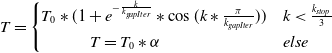 \begin{equation}T=\begin{cases} T_{0}*(1+e^{-\frac{k}{k_{\textit{gapIter}}}}*\cos (k*\frac{\pi }{k_{\textit{gapIter}}})) & k\lt \frac{k_{stop}}{3}\\ \;\;\;\;\;\;\;\;\;\;\;\;\;\;\;T=T_{0}*\alpha & else \end{cases}\end{equation}
where
 $T_{0}$
denotes the initial temperature,
$T_{0}$
denotes the initial temperature,
 $T$
denotes the temperature after the change,
$T$
denotes the temperature after the change,
 $\alpha$
is the cooling coefficient,
$\alpha$
is the cooling coefficient,
 $k$
is the number of iterations,
$k$
is the number of iterations,
 $k_{\textit{gapIter}}$
denotes the number of floating intervals, taken as
$k_{\textit{gapIter}}$
denotes the number of floating intervals, taken as
 $N$
, and
$N$
, and
 $k_{stop}$
is the preset number of iterations. Figure 8 shows a schematic diagram of the three cooling methods.
$k_{stop}$
is the preset number of iterations. Figure 8 shows a schematic diagram of the three cooling methods.
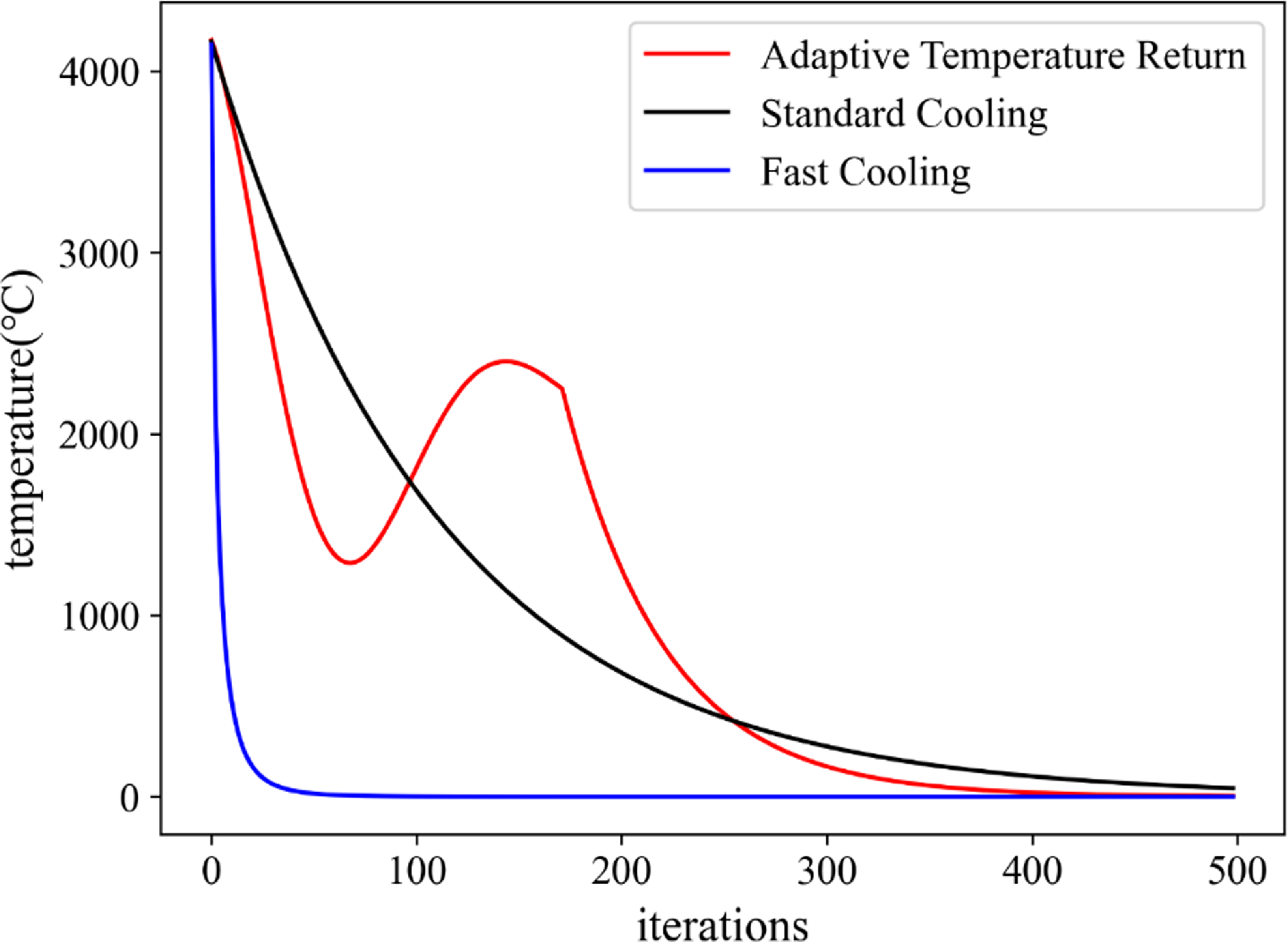
Figure 8. A comparison of the three cooling curves.
As shown in Fig. 8, the adaptive tempering introduced in this paper causes the algorithm to progress through the process of tempering and warming up during the preiteration period, thus jumping out of local optima and greatly improving the global optimization seeking ability. Moreover, repeatedly raising and lowering the temperature increases the memory function of the algorithm to maintain the optimal solution.
3.3.5 Comparison of improved SA-WOA algorithms
According to the improvement of the whale optimization algorithm based on SA algorithm in the above section, the SA-WOA coding strategy proposed in this paper is shown in Table II.
Table II. The coding strategy for SA-WOA.
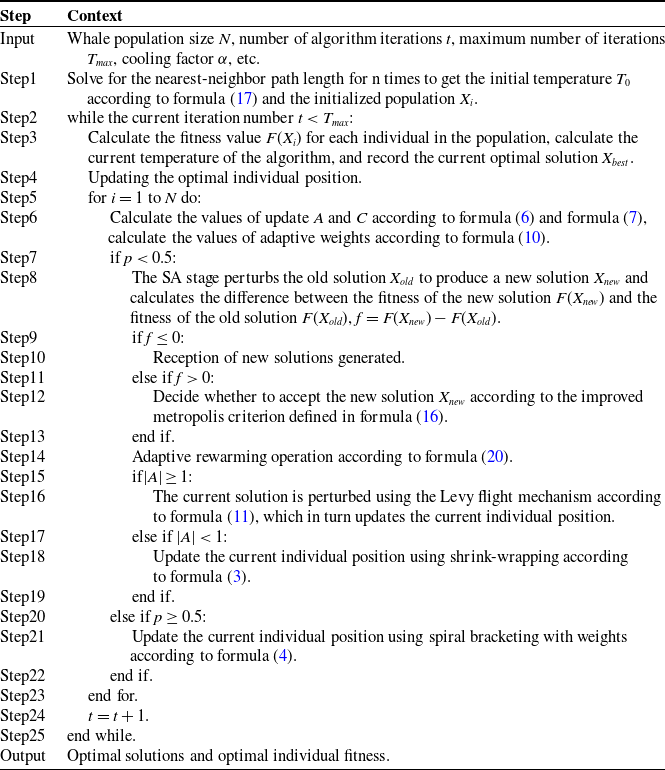
The eil76 and st70 datasets are typical datasets in the problem repository TSPLIB for the traveler’s problem and its related problems and are widely used to validate the effect of algorithmic planning for solving the TSP problem. The effect of the above-improved SA-WOA algorithm is validated using the eil76 and st70 datasets, which include the coordinate information of 76 and 70 cities, respectively, with optimal path lengths of 538 and 675, respectively. The computer used for algorithm comparison experiments in this article is the 2022 Lenovo Savior Y9000P, with an Intel core i7-12700H processor and a basic CPU frequency of 2.7 GHz. It can reach a maximum workload of 4.7 GHz and has 16 GB DDR5-4800 MHz of RAM. It is equipped with a 512 GB PCIe 4.0 SSD solid-state drive, NVIDIA GeForce RTX 3060 desktop version, and 8 GB GDDR6 graphics memory. The software running environment is PyCharm Professional 2020.1, and its configured Python version is 3.7. Typical path planning algorithms such as basic SA algorithm, whale optimization algorithm, ACA [Reference Hao, Yingnian, Jiaxing and Jing29], and particle swarm algorithm as well as improved genetic algorithm (Im-GA) [Reference Yang, Fan, Yu and Jia8] are selected for comparative analysis and 50 repetitions of each algorithm are performed using the eil76 and st70 datasets, respectively, and the number of generations of convergence and the value of convergence of each algorithm are recorded. Figure 9 shows the convergence curves of path planning using the SA-WOA algorithm of this paper for the eil76 and st70 datasets.
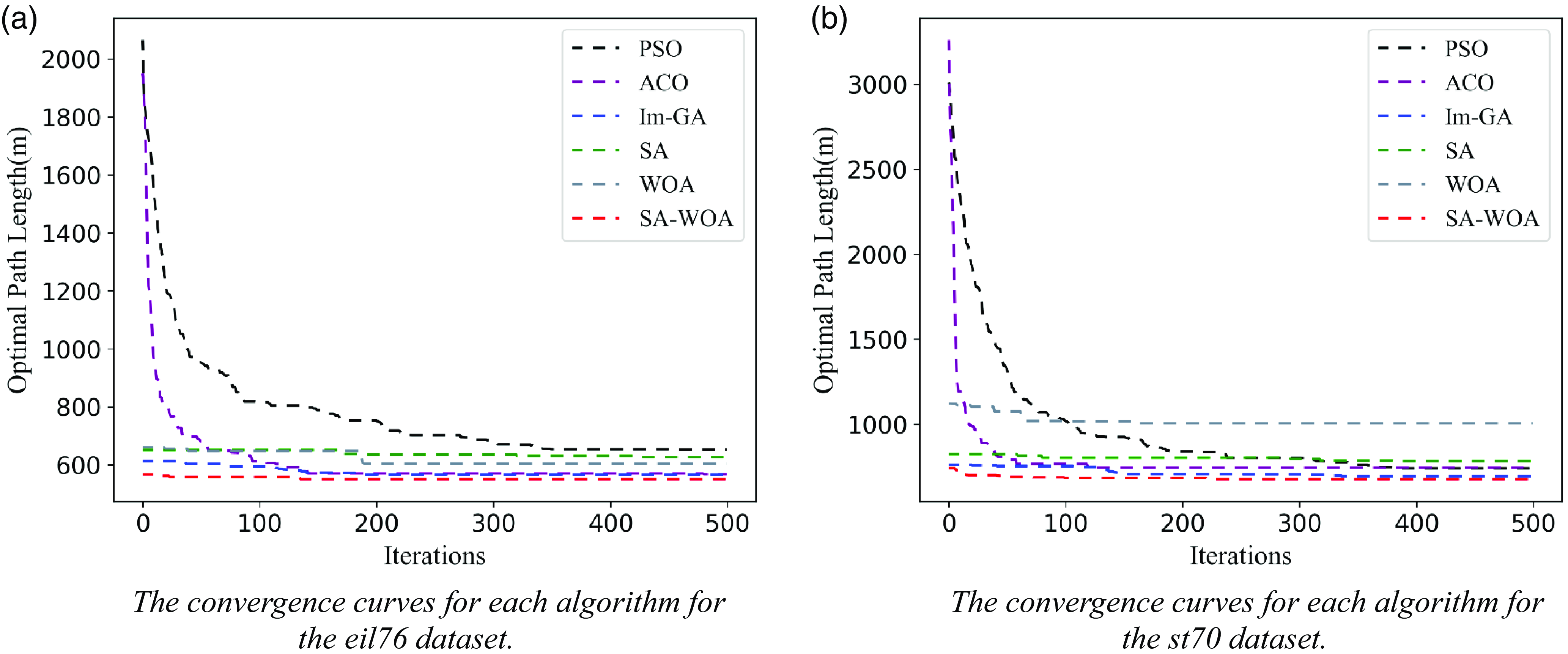
Figure 9. The algorithm comparison effect.
Meanwhile, the average number of converged generations, average convergence value, and average convergence elapsed time for 50 experiments of each algorithm are calculated, and the results are shown in Table III.
Table III. The comparison of parameters of path planning algorithm results.
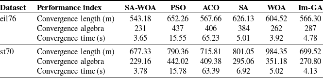
From Fig. 9, it can be seen that the improved SA-WOA algorithm in this paper has a better initial solution in path planning for both eil76 and st70 datasets, and the convergence value is significantly lower than other algorithms. From Table III, it can be seen that the average path lengths planned by the improved SA-WOA algorithm in this paper for the eil76 and st70 datasets are 543.18 and 677.33, respectively, which differ from the optimal path lengths of 538 and 675 by only 0.95% and 0.34%, respectively, and the number of convergence iterations and the convergence elapsed time are both significantly reduced. Im-GA is an improved algorithm with adaptive adjustment of crossover and mutation operators on the basis of genetic algorithm for the CPP problem in 2022. As can be seen from Table III, when comparing SA-WOA with Im-GA using the eil76 and st70 datasets in the experiments, the planning path lengths of the SA-WOA proposed in this paper are shorter by 4.08% and 3.17%, respectively, compared to the Im-GA planning lengths, and the SA-WOA uses fewer number of convergent generations and convergence time, thus validating the ability of SA-WOA to perform the novelty and superiority of SA-WOA in performing the covering path planning problem.
The computational complexity of SA-WOA in this article can be approximated as O(NGD), where N is the population size, G is the number of iterations, and D is the dimension of the solution. This complexity indicates that the running time or number of steps of SA-WOA is related to the population size, number of iterations, and the dimension of the solution. As these factors increase, the computational complexity of the algorithm also increases accordingly. It can be seen that SA-WOA is a linear computational complexity, which makes it robust in processing input data of different scales and relatively easy to scale and apply to problems of different scales. In addition, algorithms with linear complexity have efficiency and scalability, and relatively small requirements for computing and storage resources. The above results show that the improved SA-WOA algorithm in this paper can obtain better paths with fewer iterations in a shorter time and can effectively avoid falling into local optimum.
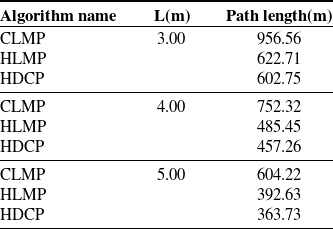
In order to evaluate the performance of this system, it was compared with the commonly used CPP methods in previous atmospheric environment monitoring work. As shown in Fig. 10, the path planning results of the Cube Decomposition Mower Path Planning Method (CLMP), Hexagonal Prism Decomposition Mower Path Planning Method (HLMP), and Hexagonal Prism Decomposition Coverage Sampling Planning Method (HDCP) for the same area are presented. Table IV shows the comparison information and simulation results of the above three methods, where L represents the coverage sampling density, L in the lawn mower path represents the side length of the square unit, and L in the other two methods represents the side length of the hexagon. From Table IV, it can be seen that under the same coverage density, the path planned by the algorithm in this paper has a shorter total flight path. This indicates that the method designed in this paper, which uses hexagonal prism sampling units for spatial sampling and SA-WOA for path planning, has good performance. It can quickly plan coverage detection paths for the fleet and save drone energy as much as possible.
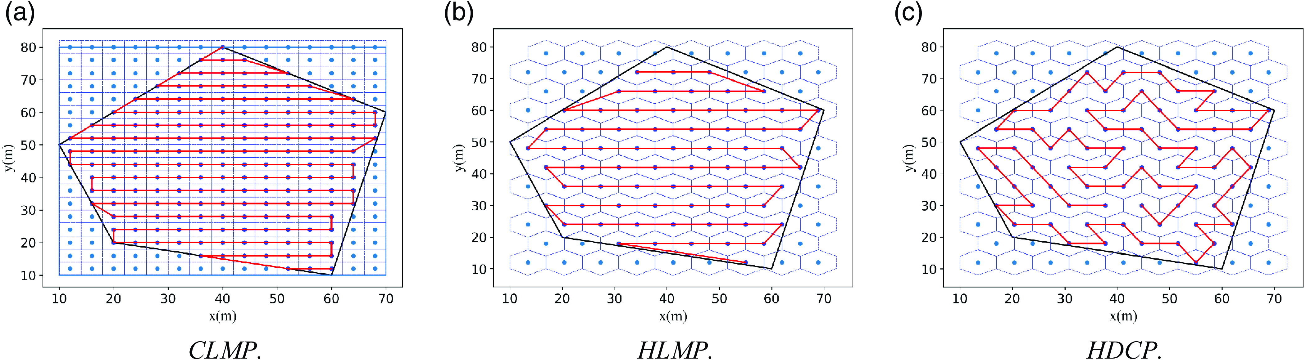
Figure 10. The planning effects of different coverage methods.
Table IV. The comparison of planning information for different coverage methods.
3.4. NURBS path smoothing
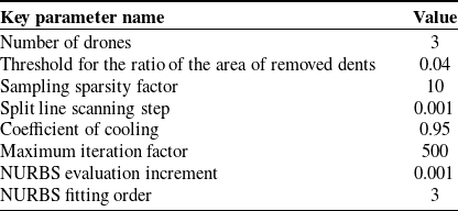
The above region partitioning and SA-WOA methods are used to conduct multi-UAV path planning tests. A convex polygonal region and a concave polygonal region are set up. The convex polygonal region has 5 vertices, and the concave polygon consists of 12 vertices with 2 concave vertices, which are assigned to 3 UAVs. The region partitioning and the path planning results are shown in Fig. 11.
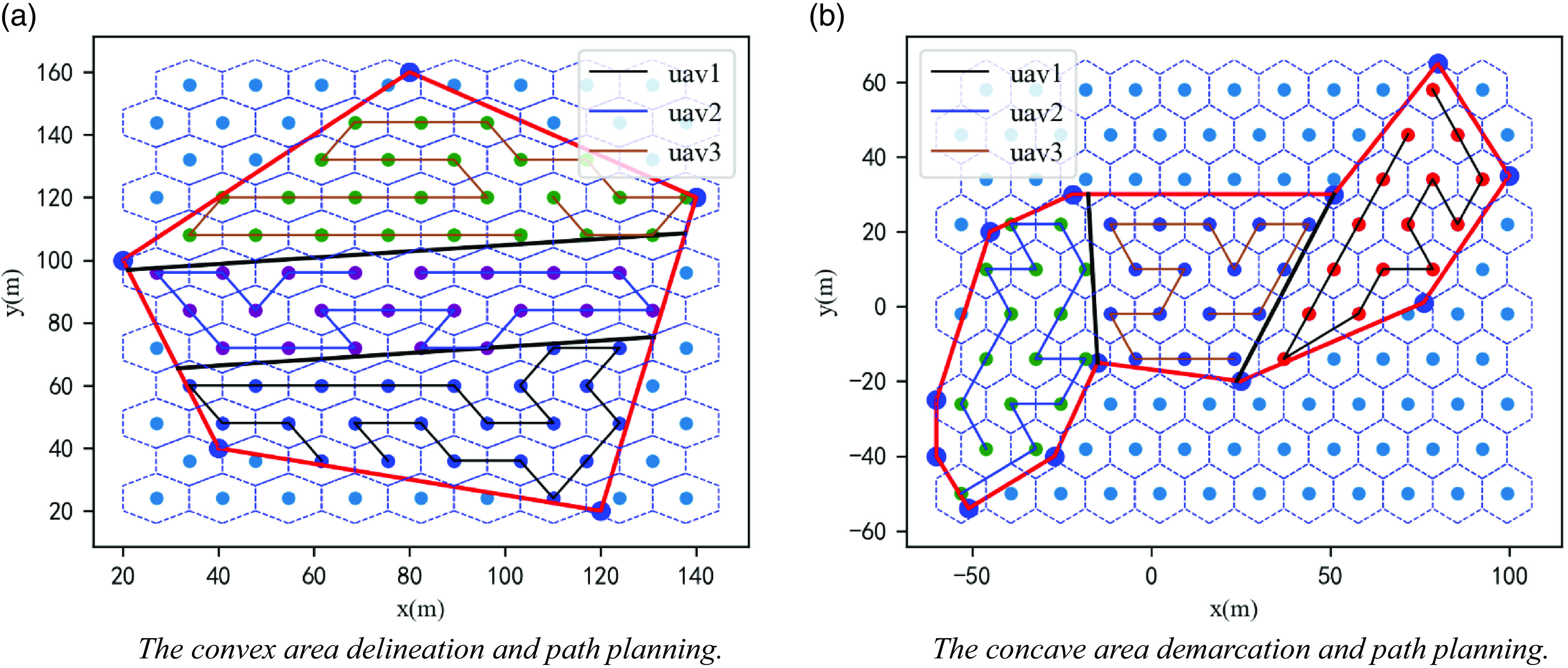
Figure 11. The multi-UAV region segmentation and path planning experiment.
As shown in Fig. 11, the paths planned using the SA-WOA do not meet the requirement of continuous UAV flight, which is second-order continuous differentiability; this leads to repeated deceleration and acceleration maneuvers at the turning points during UAV mission execution, which increases the execution time of the swarm. Therefore, the generated paths need to be smoothed to obtain the actual flight paths of the UAVs to reduce the energy loss of the UAV fleet and improve the detection efficiency.
The paths generated by the SA-WOA can be rounded using a NURBS curve, which has a very powerful and flexible shape control capability, and the small amount of interpolated data it uses makes it suitable for fast rounding of UAV flight paths [Reference Wu and Tang30].
A vector of
 $k$
th-order NURBS curves with respect to the parameter
$k$
th-order NURBS curves with respect to the parameter
 $X$
can be expressed as follows:
$X$
can be expressed as follows:
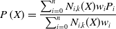 \begin{equation}P\left(X\right)=\frac{\sum _{i=0}^{n}N_{i,k}(X)w_{i}P_{i}}{\sum _{i=0}^{n}N_{i,k}(X)w_{i}}\end{equation}
which is transformed to obtain the following three-dimensional coordinates:
 \begin{equation}P\!\left(X\right)=\begin{cases} x\!\left(X\right)=\frac{\sum _{i=0}^{n}N_{i,k}(X)w_{i}x_{i}}{\sum _{i=0}^{n}N_{i,k}(X)w_{i}}\\[5pt] y\!\left(X\right)=\frac{\sum _{i=0}^{n}N_{i,k}(X)w_{i}y_{i}}{\sum _{i=0}^{n}N_{i,k}(X)w_{i}}\\[5pt] z\!\left(X\right)=\frac{\sum _{i=0}^{n}N_{i,k}(X)w_{i}z_{i}}{\sum _{i=0}^{n}N_{i,k}(X)w_{i}} \end{cases}\end{equation}
where
 $P_{i}\{x_{i},y,z_{i}\}$
are the control points of this NURBS curve,
$P_{i}\{x_{i},y,z_{i}\}$
are the control points of this NURBS curve,
 $w_{i}$
is the corresponding weight of each control point, and
$w_{i}$
is the corresponding weight of each control point, and
 $N_{i,k}(X)$
is the k-th iteration of the B-spline basis function defined in the X-direction, which is calculated as follows:
$N_{i,k}(X)$
is the k-th iteration of the B-spline basis function defined in the X-direction, which is calculated as follows:
 \begin{equation}N_{i,0}\!\left(X\right)=\begin{cases} 1, & X_{i}\leq X\leq X_{i+1}\\ 0, & \;\;\;\;\;\;else \end{cases}\end{equation}
 \begin{equation}N_{i,k}\!\left(X\right)=\frac{\left(X-X_{i}\right)N_{i,k-1}\!\left(X\right)}{X_{i+k}-X_{i}}+\frac{\left(X_{i+k+1}-X\right)N_{i+1,k-1}\!\left(X\right)}{X_{i+k+1}-X_{i+1}},k\geq 1\end{equation}
where
 $\frac{0}{0}=0$
is specified here to prevent
$\frac{0}{0}=0$
is specified here to prevent
 $\frac{0}{0}$
from occurring in the above equation.
$\frac{0}{0}$
from occurring in the above equation.
The third-order NURBS curve is used to round the planned path as shown in Fig. 11, and the effect is shown in Fig. 12.
Figure 12. The NURBS curve paths rounding.
Figure 12 shows that after rounding, the path satisfies second-order continuous minimizability; the UAV flies according to this path and only needs to adjust the roll angle and yaw angle appropriately when turning without substantial deceleration, which effectively reduces the UAV’s nonessential energy consumption and enhances the efficiency of mission execution. From the comparison between Fig. 11 and Fig. 12, it can be seen that the smooth path of the NURBS curve introduces a certain degree of path vector error, that is, the drone cannot pass through the original sampling points at certain turns, which will have a slight impact on the effectiveness of atmospheric detection. However, this error is tolerable in the use of the system in this article for atmospheric environment coverage detection in three-dimensional space. This is because the NURBS curve in this article sets the angle parameter of the curve to ensure that the smooth path is as close to the original path as possible. In Fig. 12, it can be seen that the curve at the turn is as close to the original sampling point as possible to obtain gas data around the sampling point while ensuring smoothness. Second, the effectiveness of path smoothing processing depends on the specific requirements and environmental conditions of the application scenario. When detecting the coverage of three-dimensional space, path smoothing can significantly improve the stability and comfort of flight, thereby improving the efficiency and quality of task execution. Meanwhile, the gas measurement device carried by drones continuously collects gas data during flight. Overall, the gas data measured by drones is still uniform in the space and effective in constructing the distribution of pollutants in the subsequent space.
4. Algorithm deployment and simulation experiments
The above improved SA-WOA is deployed on an NVIDIA Xavier NX equipped with UAVs, and the ROS robotics operating system is used to complete the mission planning and position control of multiple UAVs. To ensure that the designed flight trajectory meets the constraints, protects personnel safety, minimizes damage, and is capable of accomplishing the detection mission, multiple simulation experiments were conducted using the UAV simulation platform Gazebo.
4.1. Algorithm deployment
The NVIDIA Xavier NX module is an embedded AI edge computing product with a wide range of standard hardware interfaces [Reference Jablonski, Makowski, Perek, Nowakowski, Sitjes, Jakubowski, Gao and Winter31]. The ROS is an open-source meta-operating system for robots [Reference Wendt and Schuppstuhl32]. Various sensors on the robot, such as radar and GPS devices, need to transfer data to achieve reasonable control of the robot, and the implementation of process communication is the key to transferring data among them.
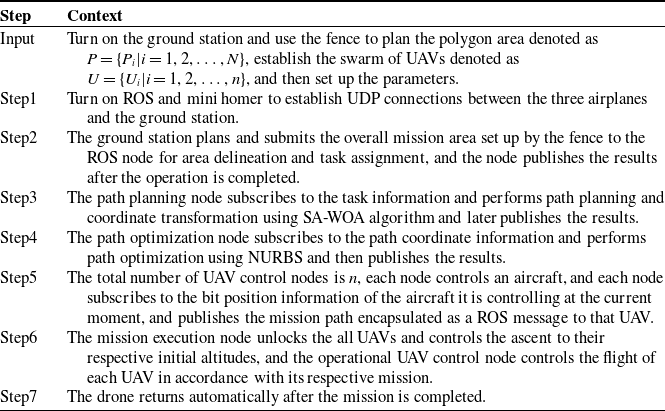
In this paper, the communication mechanism of the ROS is used to connect the first and last steps of the mission planning system as well as achieve the cooperative control of multiple UAVs, and the multi-UAV path planning algorithm is combined with the multi-UAV control system to control multiple UAVs for three-dimensional spatial environment detection. The framework of the mission planning system is shown in Fig. 13, and the planning process for the task system is shown in Table V.
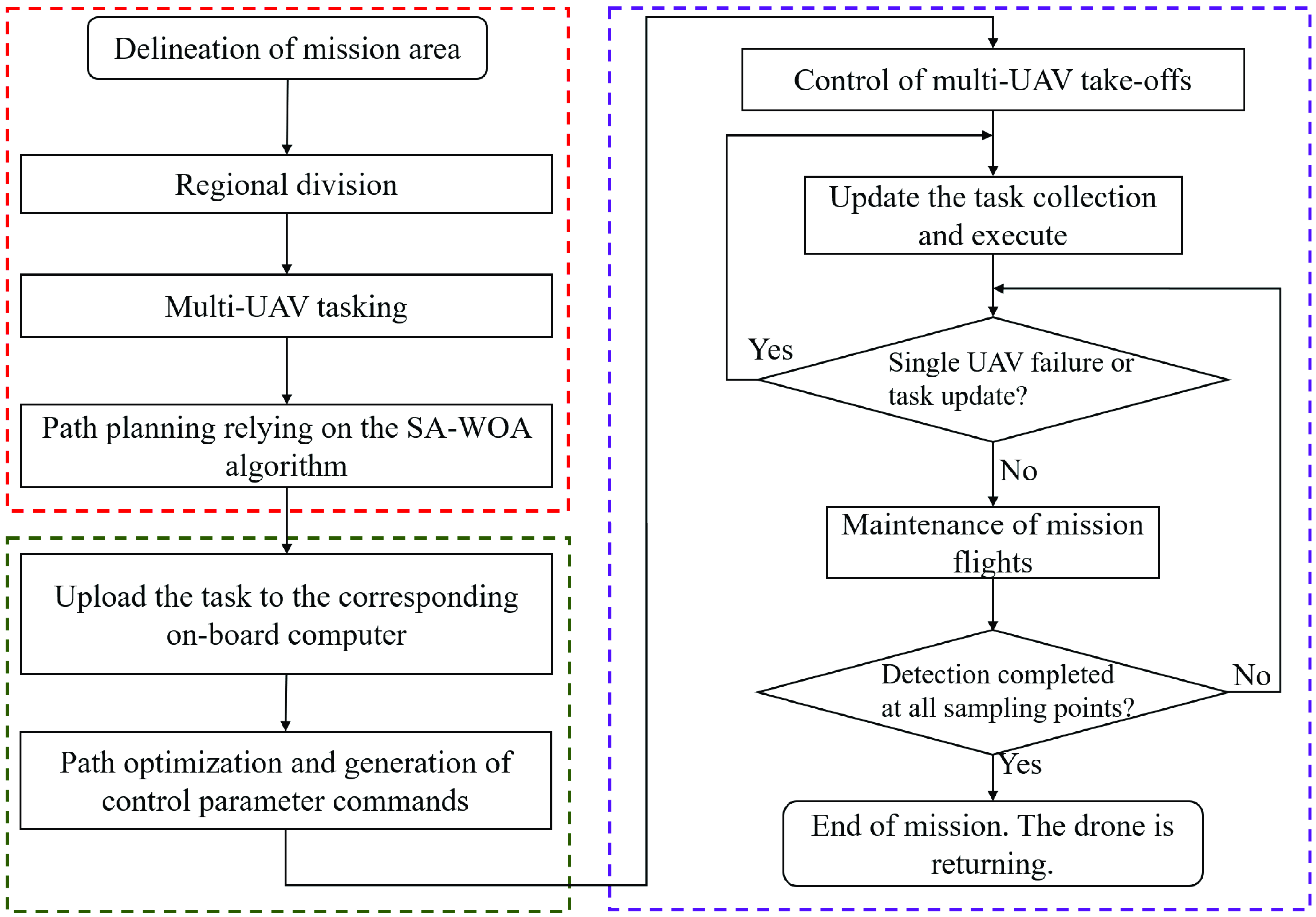
Figure 13. The mission planning system framework.
Table V. The planning process for the mission system.
During the preparation work before takeoff, the swarm of drones will run offline algorithm programs to obtain the predetermined detection path of the current drone. Each drone has its own independent ROS message and ROS node. After spatial area division, each subarea will use ROS messages from different nodes to send to different drones to avoid conflicts and ensure the safety of multiple drones. After the drone takes off, the drones in the cluster automatically publish their attitude information to the ROS core for other drones to subscribe to, ensuring mutual perception among multiple drones. When the drones in the cluster encounter some unexpected situations while performing tasks, real-time response measures need to be taken. When two drones are too close together, it is necessary to set a lower priority drone to maintain its current position and avoid the higher priority drone. When the distance between two drones becomes safe, the low priority drone’s flight mission will resume. When the drones in the cluster encounter problems and are forced to return, the remaining sampling points of the drones will be reassigned to other drones in the cluster to complete full coverage sampling of all sampling points in the space.
According to the system framework in Fig. 13, the system functions are divided into multiple ROS nodes, such as task assignment, path planning, path optimization, control interaction, and task triggering nodes, and each node completes different functional modules, which are connected to each other but do not affect each other’s operation. The system architecture of the ROS module of the multi-UAV Collaborative Space Exploration Mission Planning System is shown in Fig. 14. The functions of each node are shown in Table VI, and the types of topics used in the mission planning system are shown in Table VII.
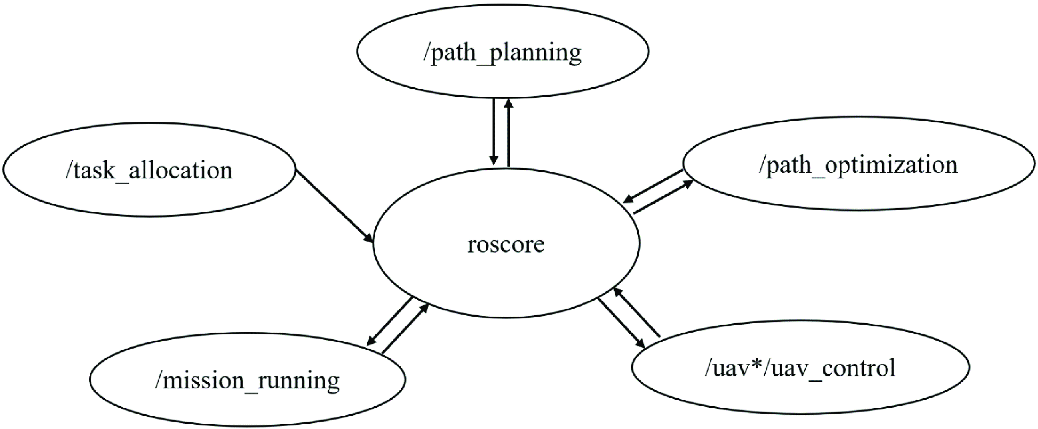
Figure 14. The ROS module message interaction.
Table VI. The functions of each ROS node in a multi-computer collaborative mission planning system.
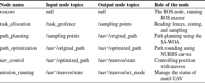
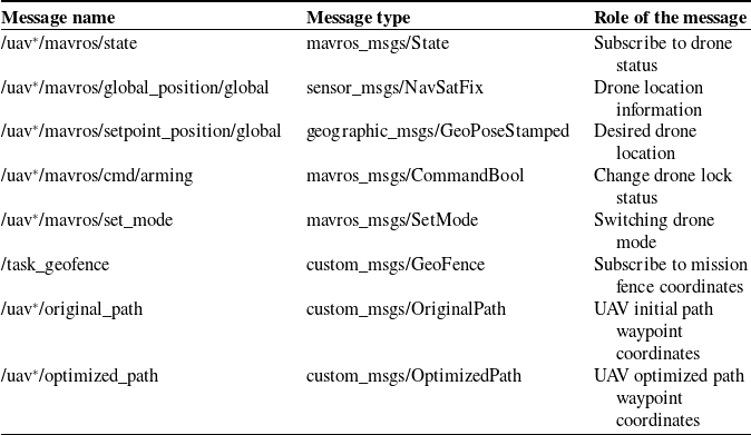
Table VII. The ROS topics and services.
After the above node and message design steps are completed, the pose control function provided by the ROS is used to control the UAV in Gazebo, after which the vehicle flies according to the algorithm-planned path to verify the effectiveness of the task planning system designed in this paper.
4.2. Multi-UAV cooperative detection simulation experiment
Gazebo is free robotics simulation software that provides high-fidelity physical simulation and a full set of sensor models used in conjunction with the ROS to provide developers with an excellent simulation environment [Reference Mitriakov, Papadakis and Garlatti33].
A multi-UAV path planning test was conducted using the above multi-UAV cooperative mission planning system, and a multi-UAV cooperative atmospheric exploration mission planning simulation and validation platform was constructed, as shown in Fig. 15.
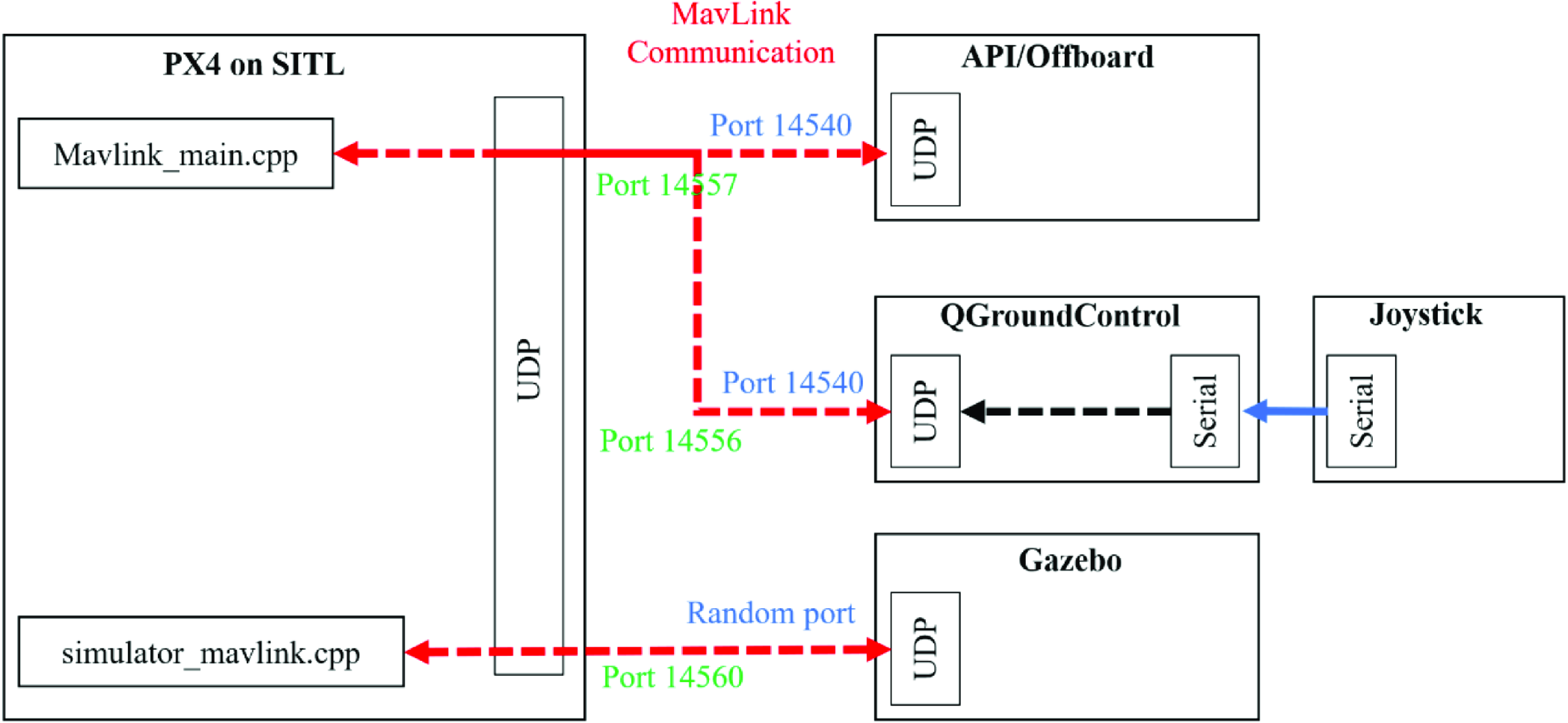
Figure 15. The simulation platform architecture diagram.
As shown in Fig. 15, the simulation platform mainly includes the Gazebo simulation platform, Pixhawk4 flight controller, and UAV ground control station. Gazebo is the core and hub of the entire system. It is connected to the Pixhawk4 flight controller through a serial port and connected to the ground station through the UDP, which communicate with each other using the MAVLink protocol. The Pixhawk4 Flight Controller, also known as the Flight Controller, is equipped with PX4 firmware and provides a quadcopter drone control model. It sends control commands to Gazebo’s drone body model, allowing the drone to complete relevant flight maneuvers based on algorithm commands. The drone ground control station can directly control the flight of the drone and can also perform autonomous flight missions. The entire simulation process can be visualized from the drone ground station and Gazebo simulation platform, such as the drone’s flight trajectory, visual images, and position status.
In the simulation experiment, the UAV swarm consists of three UAVs, and the initial position of the UAV swarm is shown in Fig. 16. In this paper, an actual flight experiment with the multi-UAV planning system is conducted by setting two kinds of nonregular stereo spaces, convex and nonconvex, near the ground station, in which the convex polygonal region has five vertices and the concave polygonal region has 10 vertices, among which there are two concave vertices, as shown in Fig. 17. The parameters of the planning system are listed in Table VIII.
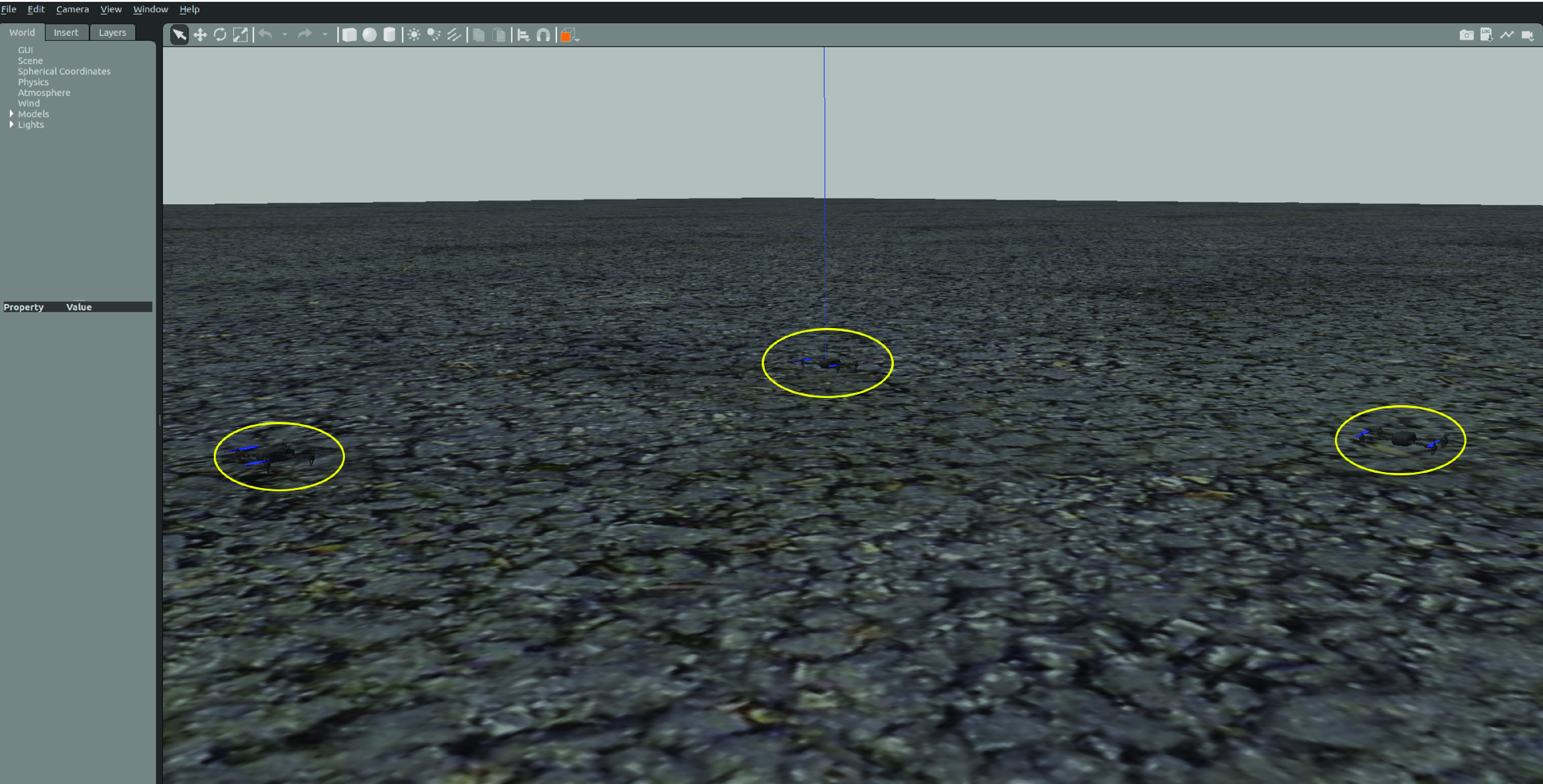
Figure 16. The initial position of the drone swarm.
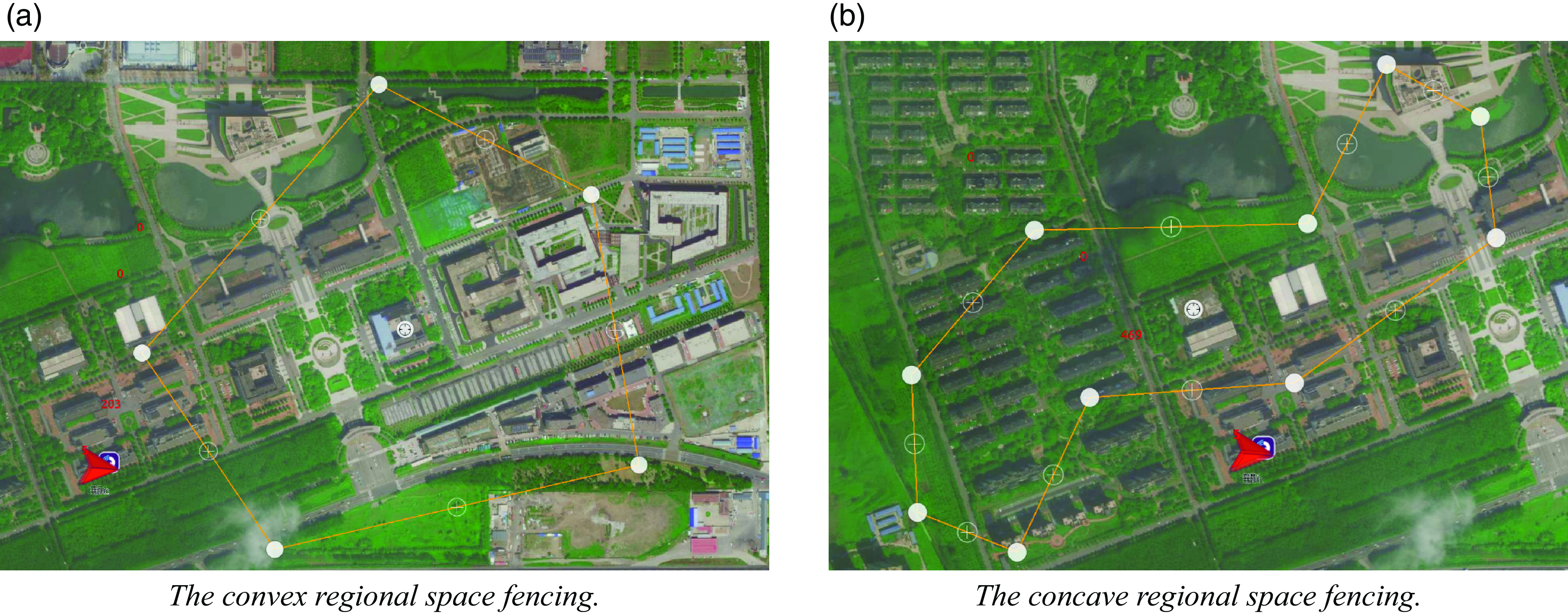
Figure 17. The fencing of space mission areas.
Table VIII. The key parameters of the planning system.
A tool called a fence is used in ground control stations to limit the flight area of drones. Fences have two categories: arbitrary polygons and circles. A safe flight area is selected for the drones by moving the turning points of the fence. When the drone flies out of this area, safety measures are triggered to make the drone hover or return to the area. This article uses this tool to plan the boundary of the vertical projection area of the target three-dimensional space at the ground station, as shown in Fig. 17. Using fences to depict this boundary can not only accurately select the task area in detail but also limit the flight space of the drone.
The spatial region shown in Fig. 17 is tasked and assigned to three UAVs, and the effects of region division and path planning are shown in Fig. 18. The third-order NURBS curves are used to round the paths shown in Fig. 18 to obtain the mission paths of each UAV, as shown in Fig. 19.
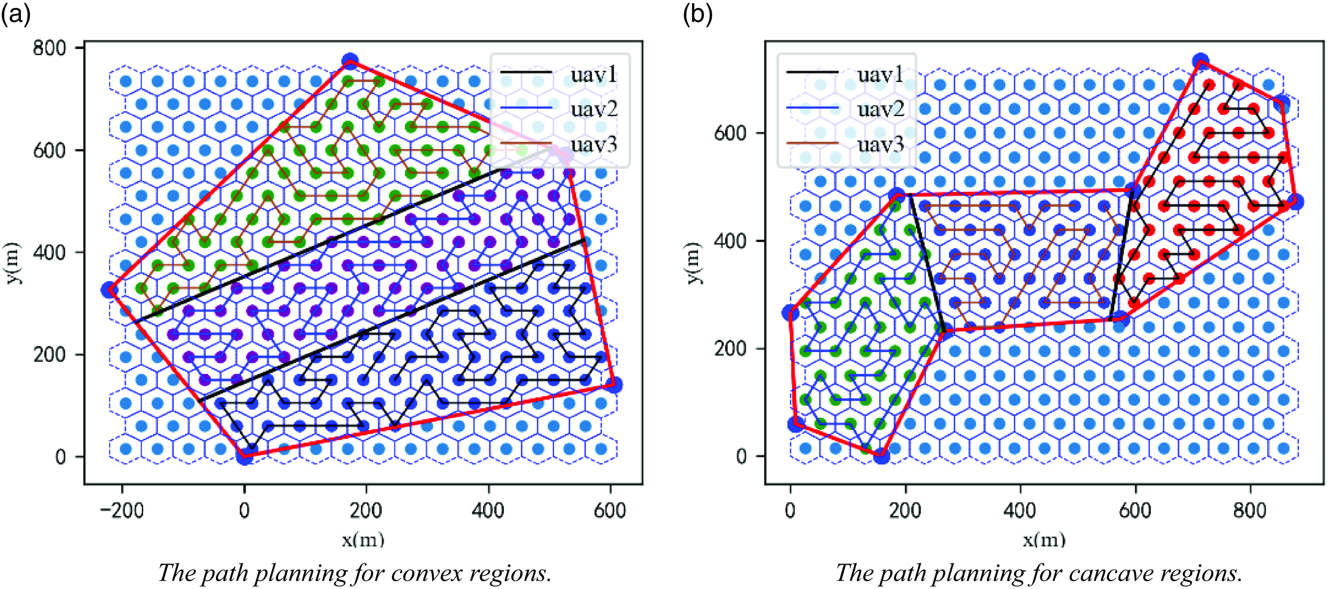
Figure 18. The fencing of space mission areas.
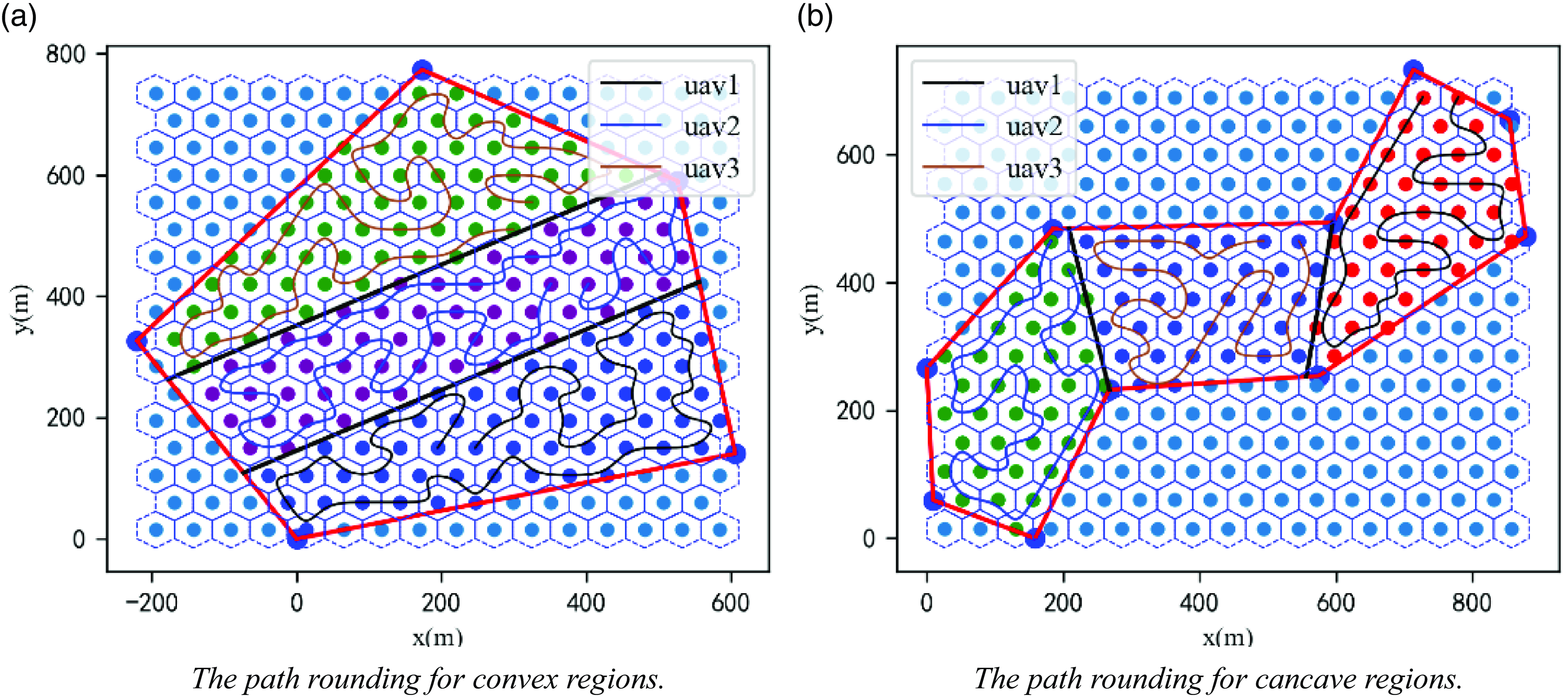
Figure 19. The fencing of space mission areas.
After solving the path planning problem of stereo space region projection, the algorithm is extended to three-dimensional space so that the mission paths of the UAVs are relatively independent and the mission path of the swarm spreads over the whole stereo space; this ensures that the swarm can detect the condition of the stereo space very well, as shown in Fig. 20.

Figure 20. The multi-UAV mission paths in three-dimensional space.
As shown in Fig. 20, the sampling and path planning for the mission area in this paper can generate a good swarm detection path; after rounding, the flight path meets the second-order continuous minimizability criterion, and the UAVs flying according to this path only need to adjust the roll angle and the yaw angle appropriately during the turn without having to perform a large deceleration operation, which effectively reduces the nonessential energy consumption of the UAVs and enhances the efficiency of mission execution. When the system completes mission planning, the result is uploaded to the ground station to generate a detection mission for each UAV, as shown in Fig. 21. The ground station used in this article was developed using QML on the basis of QGroundControl. The task planning results are displayed in the ground station view using the combined control steps of “ListView-ListModel-Delete.” ListView control is used for storing data, ListModel is used to control the format of each piece of data, and Delegate is used to display and manipulate the data in ListModel.

Figure 21. The multi-UAV stereo space exploration missions generated by the mission planning system.
The ground station is used to unify the task of turning on multiple UAVs, and the flight status of each UAV on the detection mission is shown in Fig. 22. The ground station platform used in this paper can realize real-time display of the UAV flight trajectory. The Mavlink data returned by the three drones through the ground station are analyzed via the combined control steps of "ListView-ListModel-Delete" to display their respective position information on the page. When the drone moves, ListModel increases the number of trajectory points on the drone in real time, and then Delegate control is used to connect these trajectory points into lines to visualize the real-time trajectory information of the three drones on the map. After the completion of the task, the complete flight trajectory of the UAV fleet is as shown in Fig. 22. This trajectory can be detected at the ground station along with the fences that delineate the overall task area. The system generates a three-dimensional spatial detection path, drives the UAVs to follow the predetermined flight path, and carries out multi-UAV control and trajectory display at the ground station.
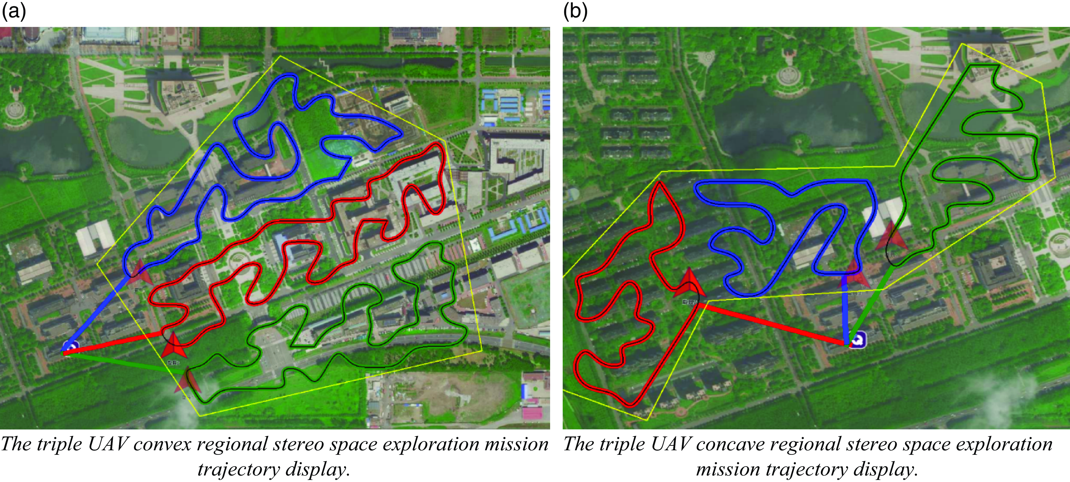
Figure 22. The ground station platform complete trajectory display.
The various results of the task assignment are shown in Table IX. The length of the task path of each UAV in the fleet is relatively balanced, and the time consumed is relatively short, indicating that the algorithm in this paper can quickly divide the area and perform path planning for the three-dimensional space.
Table IX. The experimental results of zoning and path planning.
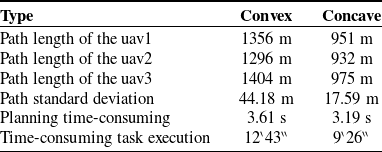
Overall, the rotorcraft atmospheric environment monitoring system and monitoring method designed in this paper are reliable and stable, provide a practical program for constructing atmospheric pollution distribution maps, and have certain practical application value and significance in three-dimensional space atmospheric environment monitoring.
5. Experimental of gas detection in stereoscopic space environment
This section mainly focuses on the measurement of environmental gases by multiple UAVs in three-dimensional spaces. First, a hardware system platform is designed and built for multi-UAV environmental detection task planning. Then, environmental gas measurement experiments are conducted, which are divided into two parts. The first part is used to verify the consistency and accuracy of the multiple gas measurement devices used in the experiment. The second part utilizes the multi-UAV collaborative CPP method to detect the environment in three-dimensional space. Finally, kriging interpolation is introduced to construct the fine-grained gas distribution in the detection space.
5.1. Multi-UAV environment detection task planning hardware platform
To complete collaborative work among multiple drones for environmental gas measurement, this article builds an environmental detection hardware implementation platform based on the aforementioned multi-UAV collaborative task planning system and the secondary development of ground control stations. The system mainly includes drone terminals, communication links, ground control terminals, and gas measurement devices, as shown in Fig. 23 [Reference Kumar, Wells, Jhawar, Ranjan and Kumar34, Reference Hou, Zha, Liu and Zhang35].
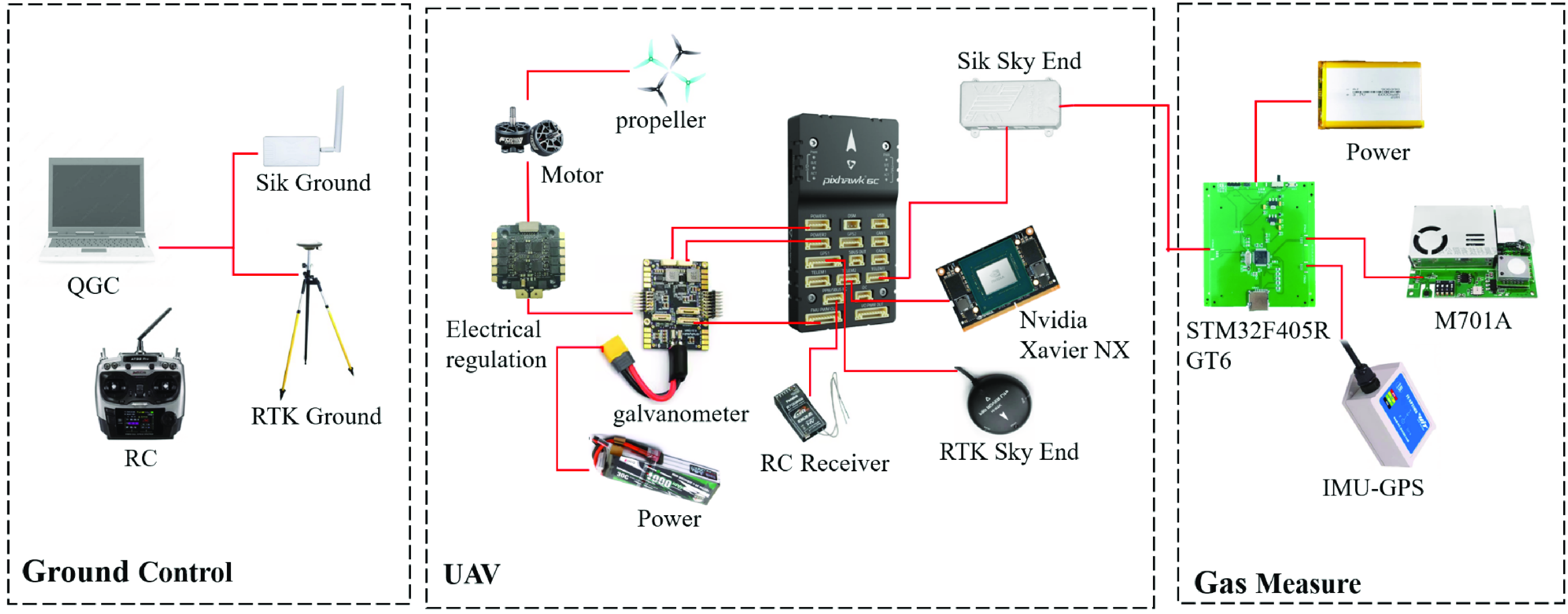
Figure 23. The multi-UAV collaborative task planning hardware platform.
The gas measurement method uses a self-assembled gas measurement device, which mainly includes a self-developed multi-sensor information core board, an M701A multi-in-one sensor air quality monitoring module produced by Shenchen Technology, and a 10-axis GPS-IMU inertial integrated navigation module produced by Weite Intelligence, as shown in Fig 24(a). The gas measurement device is assembled with the drone terminal to obtain a single drone capable of performing detection tasks, as shown in Fig 24(b). As shown in Fig 24(c), the multi-UAV experiment in this article uses three UAVs for collaborative detection, and each aircraft has the same configuration. On this basis, the communication link can be assembled to obtain the hardware implementation platform of the environmental detection system.
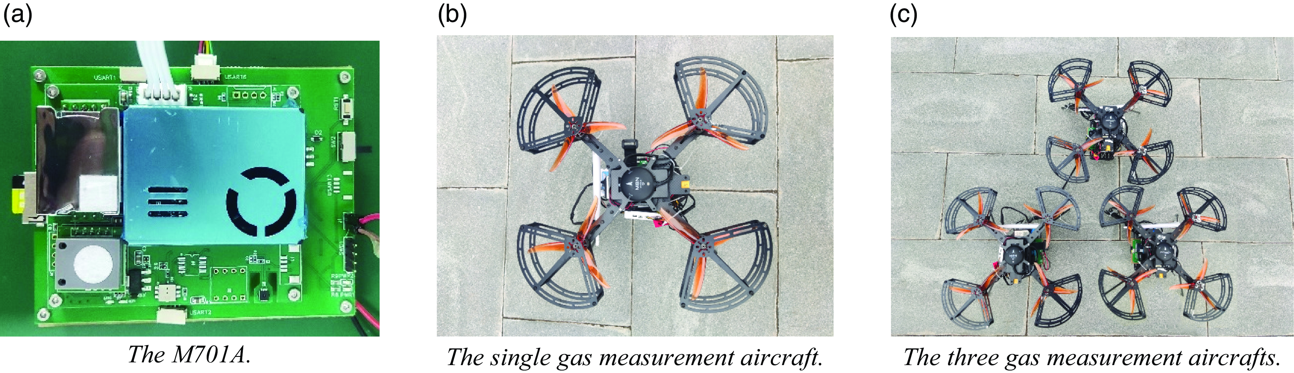
Figure 24. The gas measurement device.
5.2. Gas measurement device availability and consistency experiment
To verify the stability of the gas measurement device and the accuracy and consistency of the measurement data, a 1-week environmental gas measurement experiment was conducted. The measurement experiment was performed between 9am and 11am every day from December 16, 2023, to December 20, 2023. The GPS coordinates of the experimental location were between 115.791°E and 115.7935°E and between 37.19745°N and 37.199°N, with a relative height of 10 m to 50 m in the spatial area.
Three UAVs assembled as described above and one DJI M300RTK device carrying a Sniffer4D V2 olfactory instrument were selected for the experiment. The Sniffer4D V2 is a portable multigas monitoring device with real-time terminal data monitoring and simultaneous monitoring of multiple parameters. It can be combined with the DJI M300RTK flight platform to obtain accurate distribution information on air pollution.
The four drones were arranged evenly at the edge of the experimental area, as shown in Fig 25(a). The same flight path was set for each drone to ensure that the four gas measurement devices had a basically consistent detection environment. The predetermined flight paths of the four drones are shown in Fig 25(b). The drones flew vertically from the takeoff position and hovered at 10 m, 20 m, and 30 m to obtain results from the gas measurement devices at different heights.
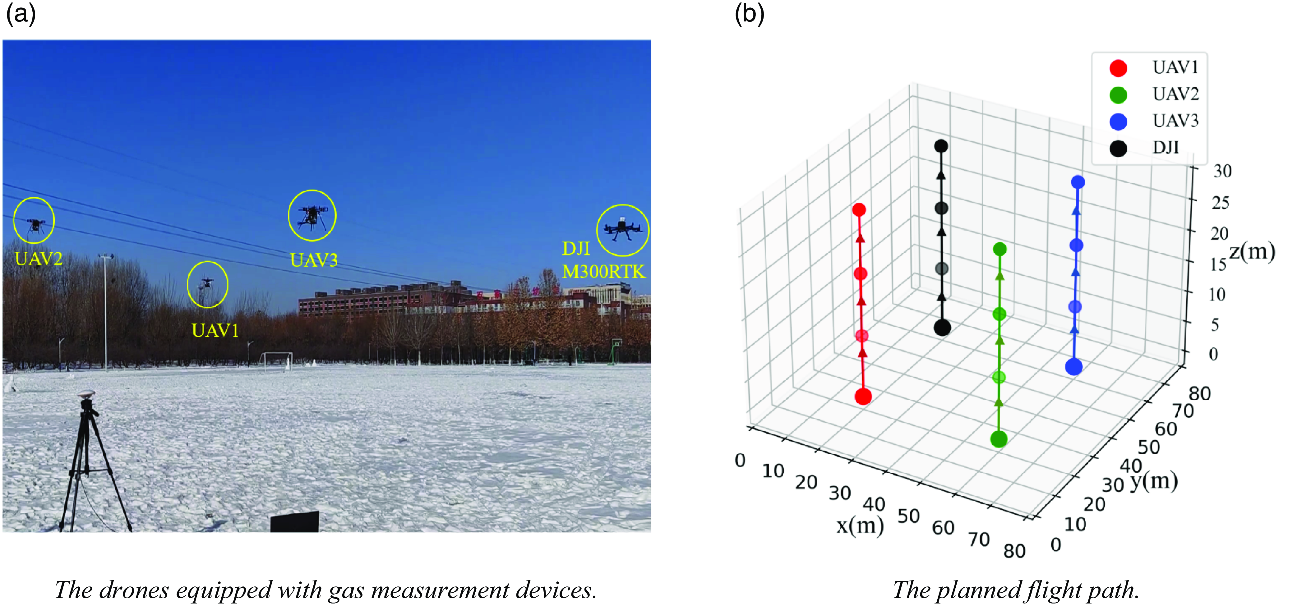
Figure 25. The consistency experiment of gas measurement device.
Another measurement experiment was conducted after 1 week. After the experiment, the daily average values of multiple gas measurement devices were taken as the concentration of atmospheric pollutants for that day. The gas measurement results of the Sniffer 4D V2 were obtained at the same time, and the air monitoring data from the Luquan No. 1 Middle School monitoring station, which is 6 km away from the experimental site, were compared. The comparison results are shown in Fig. 26. The red solid line represents the monitoring data of Luquan No. 1 Middle School, the blue solid line represents the measurement data of the olfactory system at the corresponding times, and the dotted line represents the measurement data collected by each gas measurement device designed in this article.
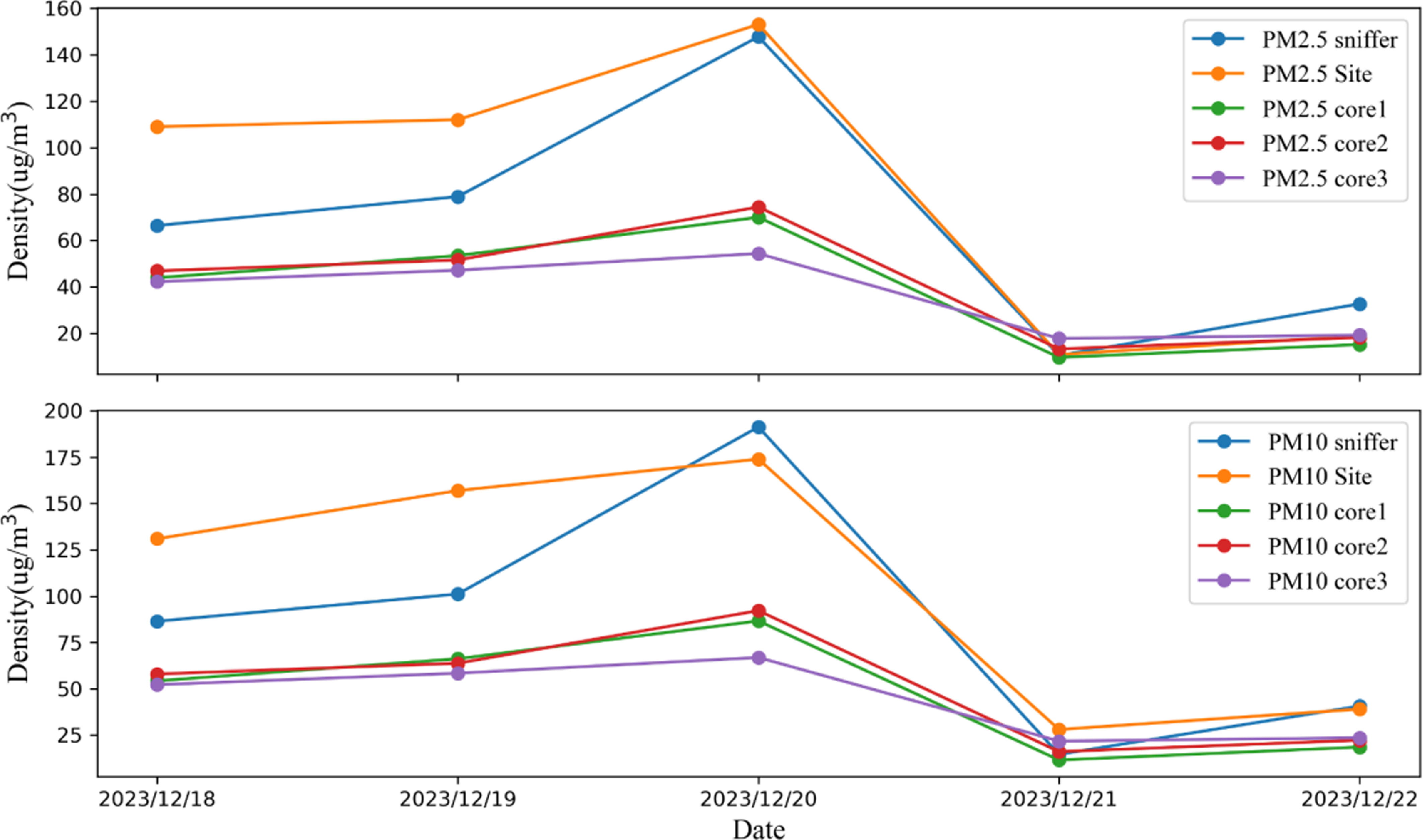
Figure 26. The comparison curve of device consistency experiment results.
To verify the accuracy of the measurements taken by the device at different heights, the PM2.5 and PM10 concentrations at each height of the three gas measurement devices during the experimental period from December 16, 2023, to December 20, 2023, were compared with the measurement data of the Sniffer4D V2 at the corresponding time and height. The comparison results are shown in Fig. 27 and Fig. 28.
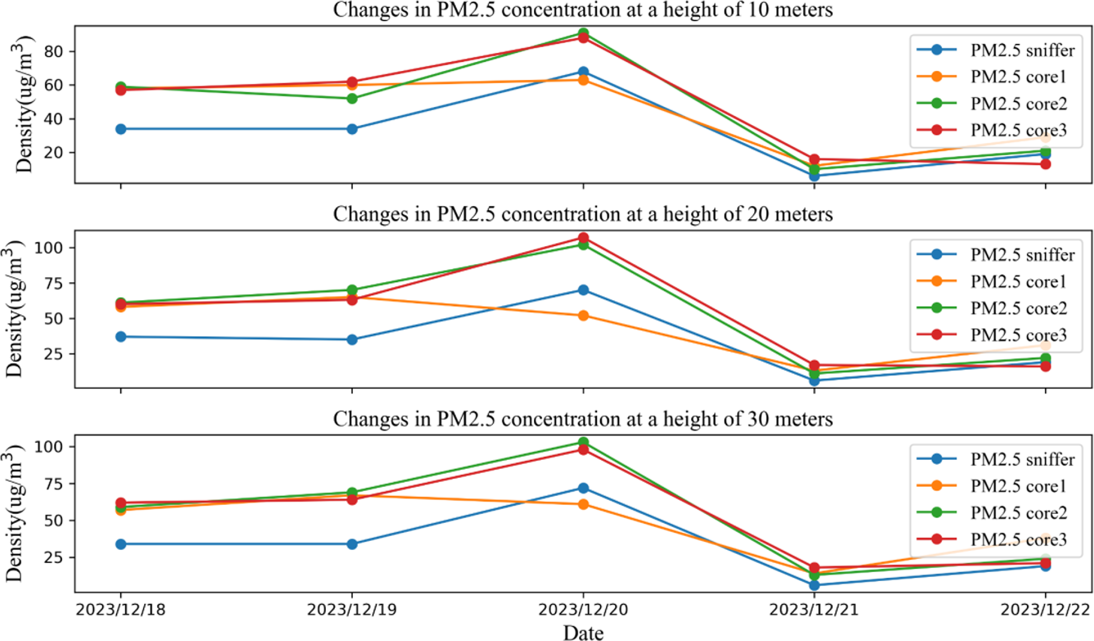
Figure 27. The comparison of consistency in results of devices with different heights of PM2.5.
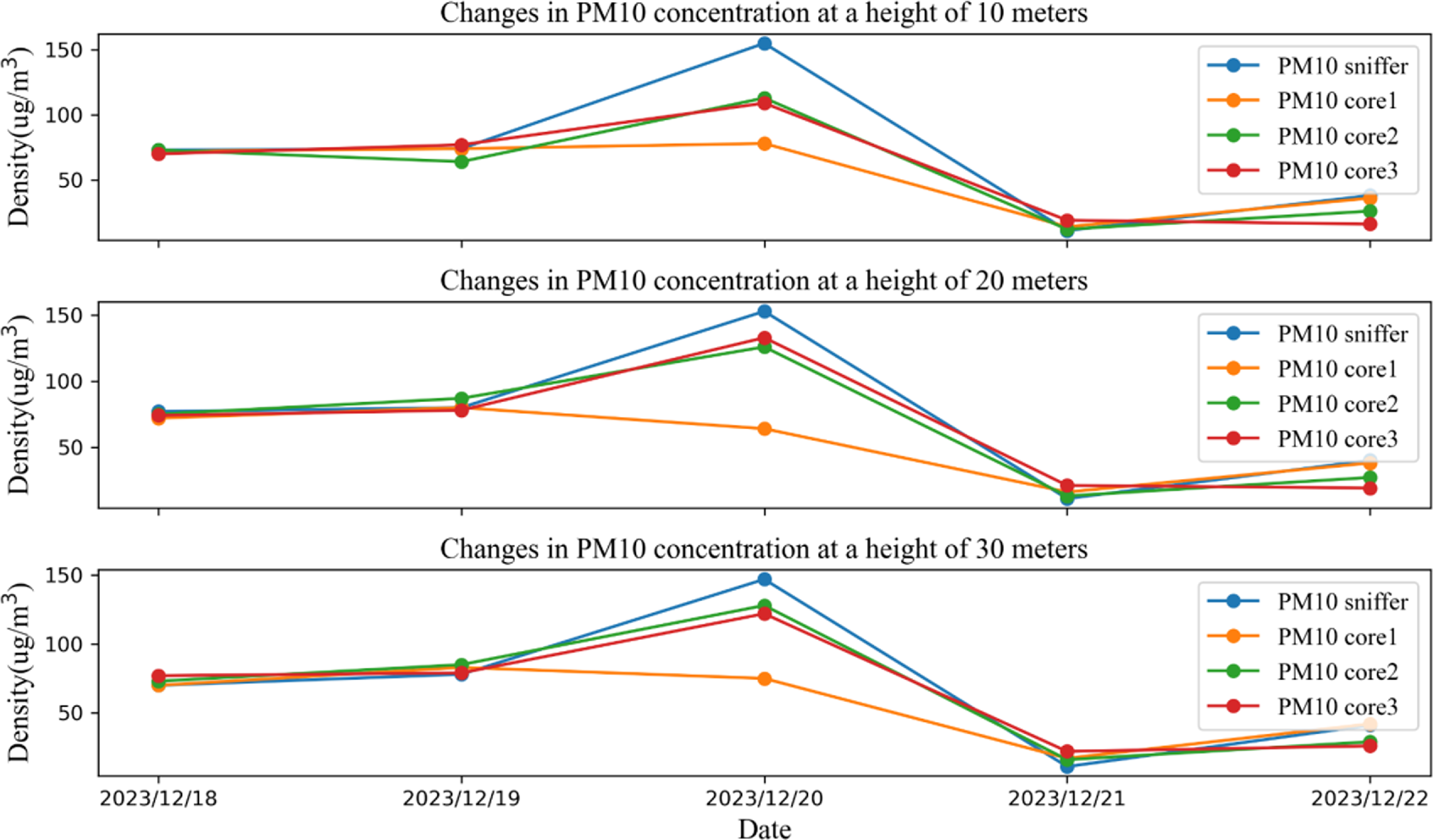
Figure 28. The comparison of consistency in results of devices with different heights of PM10.
The graph shows that although the concentrations of environmental pollutants in the experimental area detected during this study differ from the measurement results of the Sniffer4D V2 and the monitoring results at Luquan No. 1 Middle School, the daily trend in pollutant concentrations during this time period was basically consistent. The comparison of the results at different heights shows that the changes in the gas measurement device data designed in this article are basically consistent with human-detectable gas levels at each height layer, indicating that the device can effectively measure the concentration of pollutant gases at different height levels.
To further explore the accuracy and consistency of the gas measurement device designed in this article, the mean absolute error (MAE) and root mean square error (RMSE) were used to measure the differences among the data obtained by the gas measurement device designed in this period, the Sniffer 4D V2, and the monitoring station at Luquan No.1 Middle School. The average absolute error is the average absolute error between the true value and the actual measured value. The RMSE is the standard deviation between the true value and the actual measured value and is used to represent the degree of dispersion of the sample. The formulas for the MAE and RMSE are as follows [Reference Robeson and Willmott36].
 \begin{equation}MAE=\frac{1}{n}\sum _{i=1}^{n}|x_{i}-x|\end{equation}
 \begin{equation}RMSE=\sqrt{\frac{1}{n}\sum _{i=1}^{n}({x_{i}}-x)^{2}}\end{equation}
where
 $n$
represents the total number of gas samples measured in the experiment,
$n$
represents the total number of gas samples measured in the experiment,
 $x_{i}$
is the measured value of the gas samples, and
$x_{i}$
is the measured value of the gas samples, and
 $x$
is the corresponding true value of the gas data.
$x$
is the corresponding true value of the gas data.
The data from the monitoring station at Luquan No. 1 Middle School and the measurement results of the Sniffer 4D V2 were used as the actual environmental values, and the above formula was used to calculate the average absolute error and RMSE of the PM2.5 and PM10 measurements taken by the gas measurement device used in this study with respect to them. The results are shown in Tables X and XI, respectively.
Table X. The discrete results of device consistency for PM2.5.
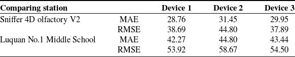
Table XI. The discrete results of device consistency for PM10.
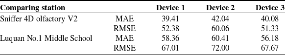
The calculated MAE and RMSE results in Tables X and XI show that the gas measurement device used in this paper has small differences from the monitoring station used at Luquan No. 1 Middle School and the Sniffer 4D V2. The RMSE and absolute mean square error of PM2.5 and PM10 are relatively small, indicating that the accuracy and consistency of the measured data are excellent. The above experimental results show that the gas measurement device designed in this article has high accuracy and consistency and can be used for subsequent collaborative detection in three-dimensional space using multiple drones and for constructing pollutant gas information distributions in the target space.
5.3. Multi-UAV collaborative three-dimensional spatial fine-grained distribution
To further study the spatial distribution of atmospheric pollutants in the experimental area, it is necessary to use the multi-UAV collaborative task planning system proposed in this paper to design a multidrone coverage flight path and use the gas measurement device designed in this paper to measure the gas at the spatial sampling points, thereby constructing a fine-grained distribution of pollutants in the target three-dimensional space.
This article uses three drones to carry gas measurement devices and sets the task area with the geofence of the ground station. With the help of the geofence, the boundaries of the task area can be flexibly delineated, and the maximum flight boundary of the drone can be restricted at the same time so that the drone will not cross the fence and the safety of the flight mission will be ensured. To verify the multi-UAV collaborative task planning system designed in this article, the overall experimental area was set within an area with GPS coordinates ranging from 115.791° E to 115.7935° E and from 37.19745° N to 37.199° N. Two irregular three-dimensional spaces, convex and nonconvex, were established with fences for actual flight experiments on multi-UAV collaborative task allocation. To verify the path planning of multi-UAV collaborative coverage in irregular three-dimensional space, the gas measurement devices carried by the three drones measured environmental gas data in the three-dimensional space.
This article delineates two types of target three-dimensional spaces, convex and nonconvex, through the secondary development of ground stations. As shown in Fig. 29, the target three-dimensional space is vertically projected to obtain a convex polygon area with six vertices and a concave polygon area with six vertices, including one concave point. The experimental height is set between 10 m and 30 m. The parameter settings of the multi-UAV collaborative task planning system are the same as those in Table VIII.
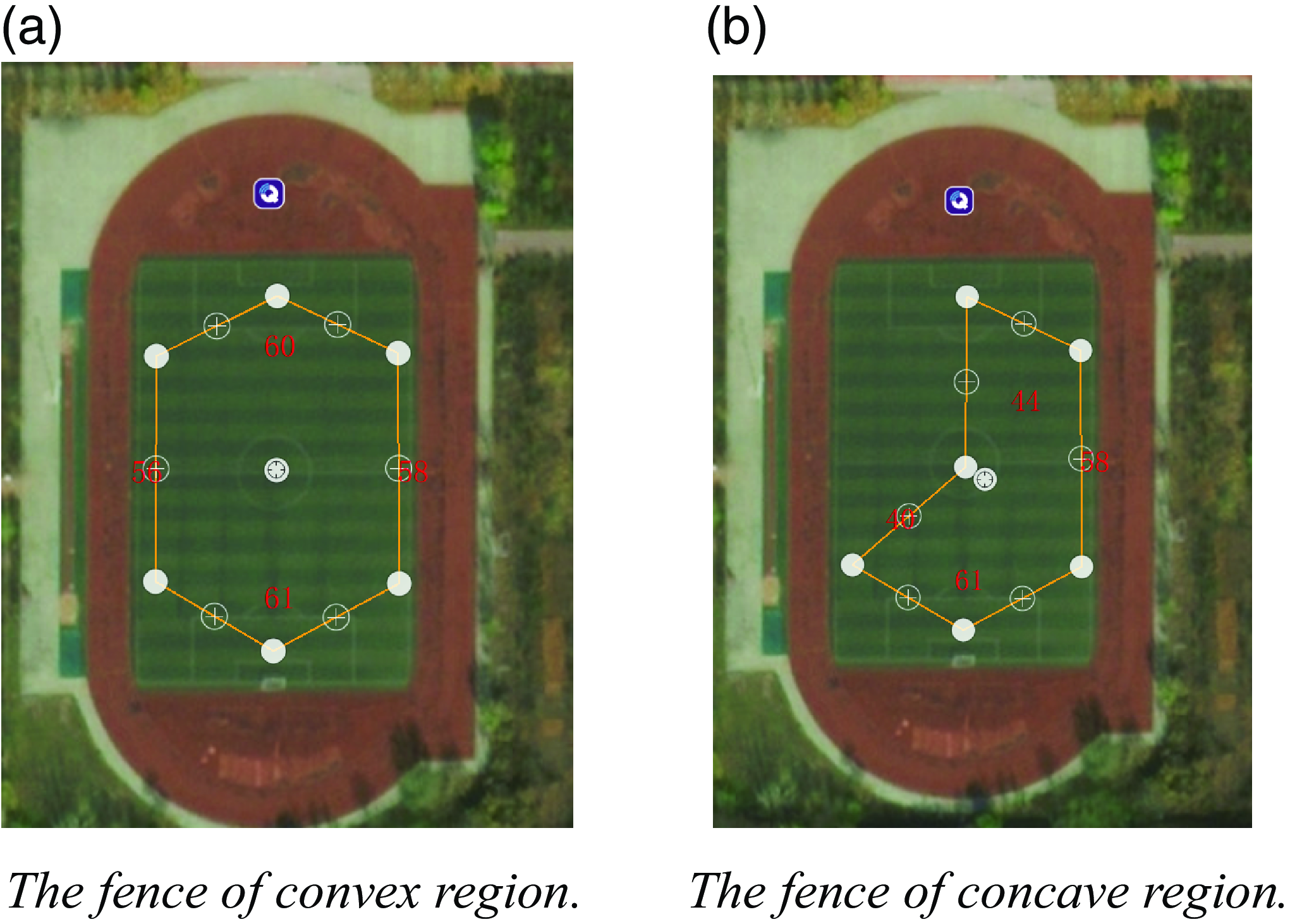
Figure 29. The fencing of the task area designated by the ground station.
The task planning system is initialized, and the modeling information of the target three-dimensional space is loaded into the system. The system automatically performs multi-UAV task planning and assigns the planned tasks to three drones. The three-dimensional detection task path of each drone after planning is completed is shown in Fig. 29. Additionally, the tasks are loaded to the ground station for subsequent cluster control of the multiple drones, as shown in Fig. 30.
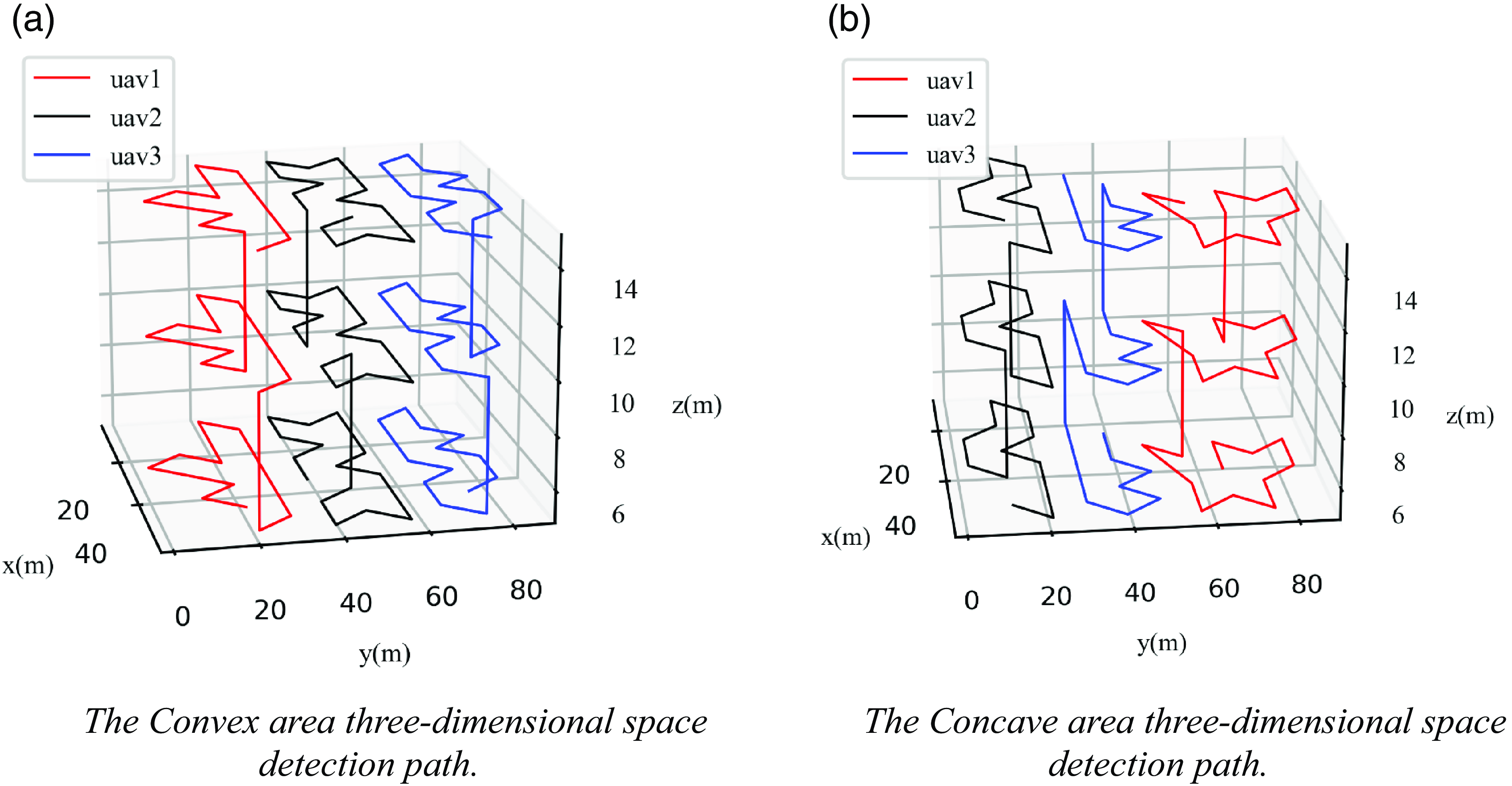
Figure 30. The planning results of three-dimensional space exploration missions.
To increase the accuracy of the flight trajectory, this article uses RTK for auxiliary positioning. The fixed RTK ground station and its analytical information are shown in Fig. 31.
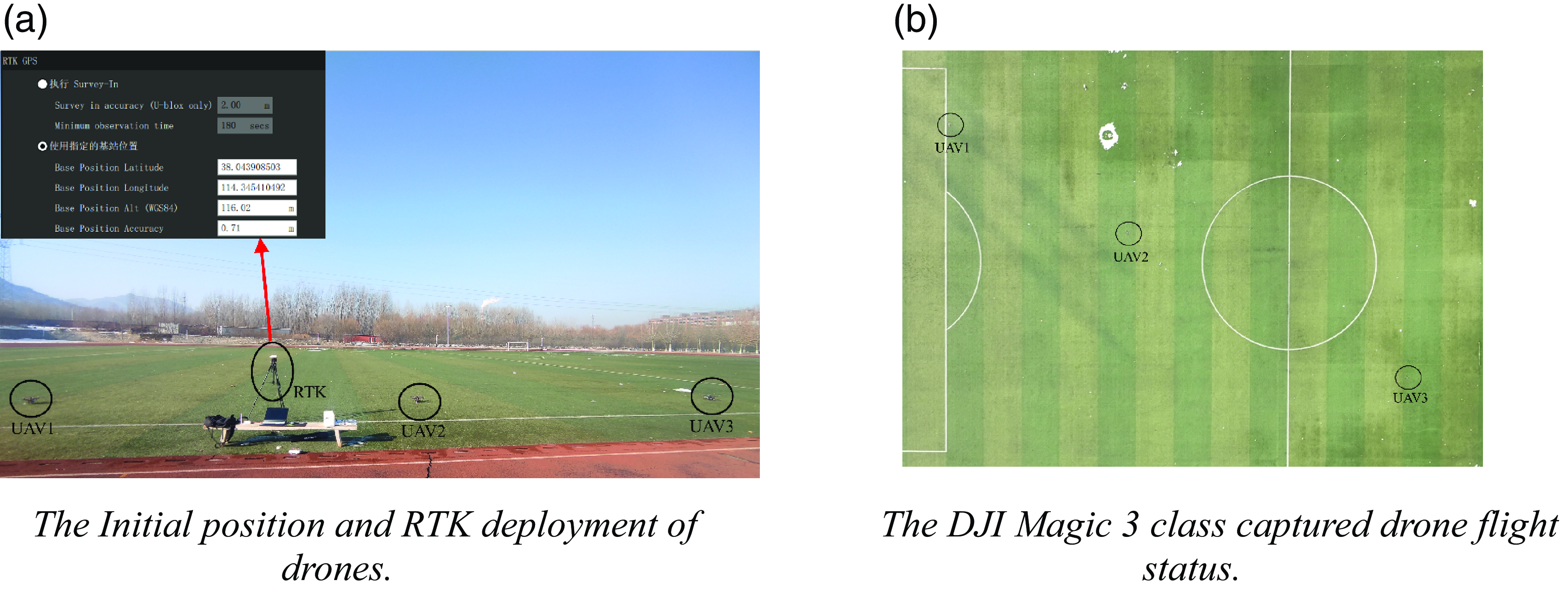
Figure 31. The actual flight scenario.
Before the exploration mission began, the DJI Mavic 3 was used to monitor the flight status and trajectory of each drone at high altitude. After the DJI Mavic 3 hovered above the mission area, the ground station was used to initiate the detection mission of the three drones. The Fig. 31(b) shows the flight status of each drone during the mission.
The ground control station designed in this article can monitor the flight parameters and pose information of multiple drones in real time. The drones hover at the sampling points for 1 to 2 s during the mission to ensure correct sampling of the planned sampling points. After all the sampling points are completed, the drones automatically return to the takeoff point. At this time, the complete flight trajectories of the three drones during the detection mission can be observed at the ground control station, as shown in Fig. 32.
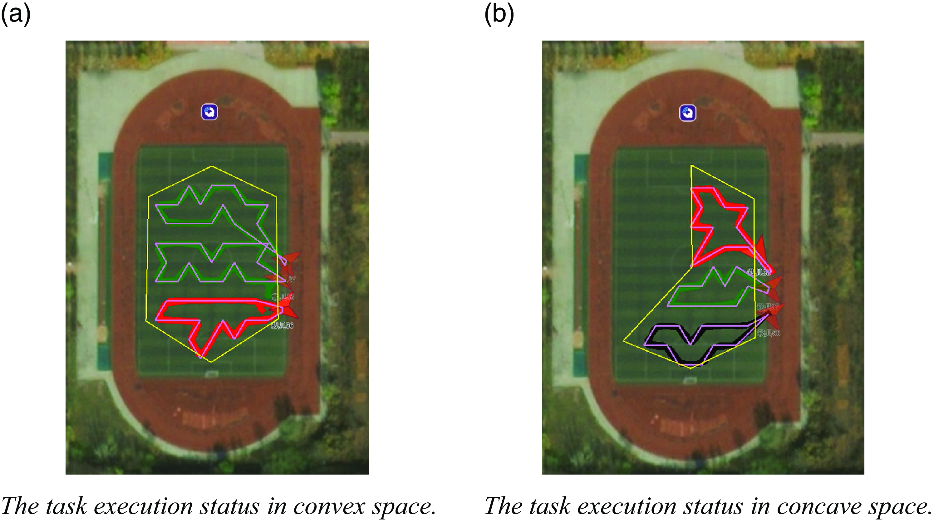
Figure 32. The task execution status displayed by the ground station.
Table XI shows the planning results and actual flight effects of the multi-UAV collaborative task planning system. The task path length planned by the task planning system for each drone in the fleet is relatively balanced, and the planning time is relatively short. This indicates that the multi-UAV collaborative task planning system designed in this article can quickly and effectively partition the target three-dimensional space and plan the path.
Table XII. The planning results of irregular stereoscopic space exploration tasks.
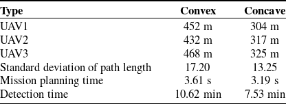
When evaluating environmental pollution in space, spatial interpolation algorithms are usually used to determine the relationship between gas concentration and spatial location to increase the accuracy of the evaluation results. Common spatial interpolation algorithms include nearest-neighbor interpolation, the radial basis function method, and kriging interpolation.
During the sampling process of the above experiment, the drone focused on hovering to take measurements near the preset sampling points, and there may not be measurement data at nonsampled points. To address this situation, we used the kriging interpolation method to reconstruct the relationship between gas concentration and spatial position in the target three-dimensional space. The kriging interpolation method is a regression algorithm that can model and predict random processes in space. The interpolation process considers not only the relationship between the predicted point and the given data point’s spatial position but also the spatial correlation of the predicted points, thereby minimizing the error between the estimated value of the unknown position and the true value [Reference Rusmili, Hamzah, Choy, Azizah, Sulistyorini, Yudhastuti, Diyanah, Adriyani and Latif37].
The kriging interpolation method uses the weighted sum operation on data from known points in space to estimate the data of unknown points. The estimation formula is as follows:
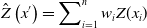 \begin{equation}\hat{Z}\left(x'\right)=\sum\nolimits_{i=1}^{n}w_{i}Z(x_{i})\end{equation}
Here,
 $x'$
is an unknown prediction point,
$x'$
is an unknown prediction point,
 $\hat{Z}(x')$
is the estimated value,
$\hat{Z}(x')$
is the estimated value,
 $Z(x_{i})$
is the measured value of a known point in space, and
$Z(x_{i})$
is the measured value of a known point in space, and
 $w_{i}$
is the weight factor of the measurement value, which represents the ability of the current measurement value to affect the final estimated value. The value of the weight factor is determined jointly by the estimated value and the measured value. The weight factor corresponding to each measurement and value should satisfy the estimated value at
$w_{i}$
is the weight factor of the measurement value, which represents the ability of the current measurement value to affect the final estimated value. The value of the weight factor is determined jointly by the estimated value and the measured value. The weight factor corresponding to each measurement and value should satisfy the estimated value at
 $x'$
. The coefficient that minimizes the variance between
$x'$
. The coefficient that minimizes the variance between
 $\hat{Z}(x')$
and the measured value
$\hat{Z}(x')$
and the measured value
 $Z(x')$
should also satisfy the condition of unbiased estimation, as shown in the following equations:
$Z(x')$
should also satisfy the condition of unbiased estimation, as shown in the following equations:
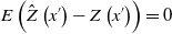 \begin{equation}E\left(\hat{Z}\left(x'\right)-Z\left(x'\right)\right)=0\end{equation}
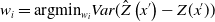 \begin{equation}w_{i}=\text{argmin}_{{w_{i}}}Var(\hat{Z}\left(x'\right)-Z(x'))\end{equation}
Based on the above experiment proving that the measurement data and position of the gas measurement device are correct, the gas data measured in this experiment are used to construct the fine-grained distribution of pollutants in the target three-dimensional space. Because the gas measurement device hangs below the rotor aircraft, rotor disturbance during rapid flight can affect the gas distribution around the drone, thereby affecting the measurement results. To minimize the impact of rotor disturbance, the drone is set to hover at the sampling point position because a hovering drone has a more stable surrounding airflow than a moving drone, making the measurement data more accurate.
The pollutant concentration data of all the sampling points were selected in this experiment, and the kriging interpolation method was used to generate an environmental pollution distribution map of the target three-dimensional space. Due to the relatively small airflow influence between each sampling point, the pollutant concentration in the spatial distribution is more in line with the Gaussian distribution. Therefore, in the kriging interpolation process, a Gaussian-type variation function is selected for interpolation operation prediction, the PM2.5 and PM10 concentrations are interpolated in the three-dimensional space of the concave and convex regions, respectively, and their distributions in the horizontal and vertical directions are analyzed. The results are shown in Fig. 33 and Fig. 34.

Figure 33. Distribution of pollutants in convex three-dimensional space.
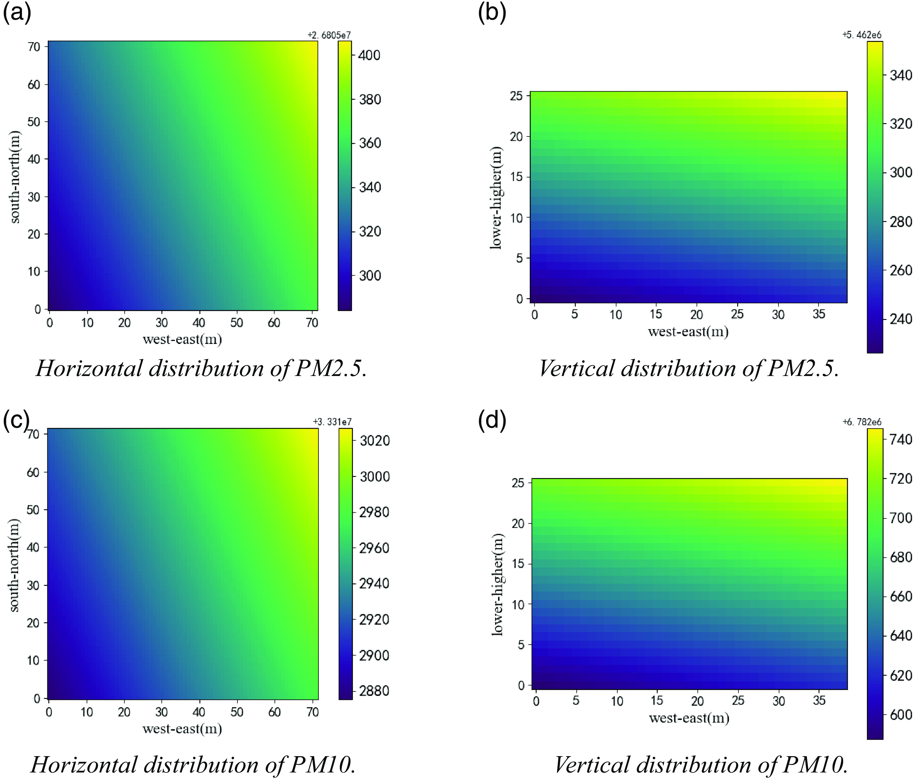
Figure 34. Distribution of pollutants in concave three-dimensional space.
From Figs. 33 and 34, it can be seen that the distribution of pollutants in the target three-dimensional space is the same. Although it is at the same location, the multi-UAV collaborative detection experiment on the three-dimensional space was not conducted in the same concave convex area set on the same day. Considering the different weather conditions in the 2 days, there are differences in the distribution of pollutants in the same space constructed through the multi-UAV detection experiment in the concave convex area. However, there is no significant difference in the distribution of pollutants in the space reflected in Figs. 33 and 34. From the horizontal interpolation results, it can be seen that the concentration of pollutants gradually increases from west to east at the same horizontal height. From the vertical interpolation results, it can be seen that the concentration of pollutants gradually increases with the increase in height. This is due to the lower terrain of the playground where the experimental site is located and the presence of a school’s teaching building, experimental building, and traffic lane on the east side. Therefore, under the influence of vehicles and a large number of personnel flow, the pollutant concentration on the east side of the experimental site is significantly higher than that on the west side and increases with height. The overall experimental results indicate that the multi-UAV collaborative atmospheric environment detection system designed and constructed in this paper is feasible and stable and can quickly complete the atmospheric environment detection task of multiple UAVs in the three-dimensional space of the target. It has high application value in the measurement of atmospheric environment quality in three-dimensional space.
6. Conclusions and future work
In this paper, for the application of multi-UAV cooperative environmental exploration, the division of nonregular stereo spatial region, sampling, and the path planning method of full domain coverage are studied, and a multi-UAV cooperative environmental exploration mission planning system is designed. First, the target three-dimensional spatial region is divided by graphical decomposition, and each subspace is decomposed and sampled by hexagonal sampling units to obtain a collection of sampling points covering each subspace. In the CPP of these sampling point sets, this paper proposes a SA-WOA, and with the help of the eil76 and st70 datasets, SA-WOA is compared with the basic SA, WOA, Im-GA, and other algorithms respectively, and the results show that the planning length of SA-WOA algorithm is 10.15% and 31.19% shorter than that of the WOA planning results for the two datasets, respectively, 13.25% and 15.44% shorter than SA planning results, 4.08% and 3.17% shorter than Im-GA planning results, and only 0.95% and 0.34% difference from the optimal path length corresponding to the dataset. Compared with other algorithms, SA-WOA is in the optimal position in terms of the number of convergence generations and convergence time, which is sufficient to prove that SA-WOA has good feasibility and novelty. After using SA-WOA to plan the paths for each collection of sampling points, these paths are smoothed using NURBS curves to obtain the coverage mission paths that satisfy the continuous flight of the UAV. The system is validated using the Gazebo simulation platform, and then the hardware implementation platform of the multi-aircraft collaborative environmental detection system is constructed and a 1-week environmental gas measurement experiment and target stereo spatial coverage detection experiment are carried out. The experimental results show that the concentration data of PM2.5 and PM10 measured by the gas measurement device used in this paper are consistent with the trend of the monitoring data from the monitoring stations of Sniffer 4D olfactory V2 and Luquan No.1 Middle School, and the atmospheric pollutant distribution maps of the target three-dimensional space are constructed using the kriging interpolation method, which verifies that the multi-UAV collaborative environmental detection mission planning system designed in this paper can rapidly detect and construct the pollutant distribution map of the target nonregular three-dimensional space, which is of practical value and significance for the research of multi-UAV collaborative technology in the field of atmospheric environmental pollution prevention and control.
Future research can be conducted in several directions. One is to optimize the system architecture, carry out product upgrades, and achieve a multi-UAV collaborative task planning system that integrates emergency takeoff, portable monitoring, and space gas distribution construction. Second, environmental factors such as wind speed and temperature can be taken into account in the energy consumption of UAVs so that the system can stably and effectively carry out task planning and environmental detection in different emergency environments. Finally, the collaborative communication mechanism between multiple drones can be optimized to ensure the security of task execution.
Author contributions
Binggang Yu and Shurui Fan conceived and designed the paper. Binggang Yu, Weijia Cui, and Kewen Xia conducted paper gathering. Binggang Yu, Shurui Fan, Weijia Cui, and Li Wang wrote the article.
Financial support
The research was supported by the National Natural Science Foundation of China (No.42075129), Key Research and Development Project from Hebei Province of China (No.19210404D, No.SJMYF2022Y06, No.21351803D).
Competing interests
We declare that we have no known competing financial interests or personal relationships that could have appeared to influence the work reported in this paper.
Ethical approval
None.


