1. Introduction
Parallel robot consists of a fixed platform and a moving platform that are connected by several limbs. This leads to a compact structure and high potential stiffness; however, it also results in a complex relationship between motions and constraints. In fact, motions and constraints are crucial factors in kinematic and stiffness modeling. Moreover, the number and properties of mobility can be determined by considering motion and constraints. Hence, analyzing motion and constraints automatically by programming is a fundamental task in computer-assisted mobility analysis and performance modeling.
In screw theory [Reference Huang, Li and Ding1–Reference Hunt2], if a wrench acts on a rigid body in such a way that it produces no work on its infinitesimal twist, the two screws are referred to as reciprocal. The reciprocal product is an algebraic operation defined as a scalar product based on the virtual power of a wrench on a twist. This product is zero between motion and its constraints [Reference Huang, Li and Ding1]. So far, solving for motion and constraint has been a null space problem that has been well studied in mathematics. The null space can be found using various numerical methods, such as Gauss–Seidel elimination [Reference Meyer3], Gram–Schmidt orthogonalization [Reference Sugimoto and Duffy4], and an affine augmentation method [Reference Dai and Jones5]. However, it is noted that there are multiple solutions when the screw system is lower than five-dimensional, making it difficult to select solutions with explicit physical meanings. Although any selected solution would result in the correct number of degrees of freedom (DoF), it may lead to incorrect properties and confused results in performance modeling. Nevertheless, in automatically solving motion and constraints [Reference Ding, Cao, Cai and Kecskeméthy6], it is necessary but difficult to generate initial motion axis screws in algebraic format relative to a same coordinate system.
The observation method is an alternative approach that investigates the kinematic features of some typical joints and branches to determine the constraints. Hunt discussed the relationship between three-dimensional geometry and spatial mechanisms in the context of a simplified screw system [Reference Hunt2]. An analytical approach to determine the bases of three unknown twist and wrench subspaces of lower mobility serial kinematic chains was presented, stemming from the reciprocal product of screw theory [Reference Huang, Yang, Wang, Sun and Chetwynd7]. Thanks to progress made in recent years, the typical geometric conditions for motion and constraints have been determined. These conditions are as follows: the translational motion axis should be perpendicular to the constraint force, and the rotational motion axis should intersect with the force constraint and be perpendicular to the couple constraint. Building on these ideas, Yu proposed a graphical approach that visualizes motion and constraints [Reference Pei and Yu8]. Additionally, a geometric algebra approach was presented to determine the motion, constraint, mobility, and singularity of parallel mechanisms [Reference Huo, Sun and Song9]. The observation method involves several rules that can be realized through reasoning, such as the “IF…THEN…” type. However, this automatic manner can only be applied to simple cases where only one rule is involved. Alternatively, Liu subsequently deposits the frequently used results of serial kinematic chains from observation and proposed an automatic approach for identifying the natural reciprocal screw systems based on the invariance properties of topology [Reference Liu, Kecskeméthy and Huang10]. But for the cases out of these templates, it is hard to achieve the solution.
When carrying out automatic constraint and motion analysis, we always translate the known formulas, rules, or cases into computer language. However, this “translating manner” is limited to mechanisms within the known ones. In fact, constraint and motion analysis involves learning and reasoning, which are not independent of the experience and intelligence of people and cannot be realized by programming alone. Machine learning, on the other hand, is known for its reasoning abilities and can perform these thinking processes, making it well suited to automatic motion and constraint analysis. If the explicit meanings of the reciprocity between twist and wrench are learned by machine learning, constraint problems can be quickly and visually solved. Currently, machine learning is closely related to robotics, but it is mostly used for trajectory planning, cognition, control algorithms, and some fields of structural optimization [Reference Atmeh and Subbarao11–Reference Freitag, Peters, Edler and Meschke13]. In this case, a dataset indicating explicit meanings of the reciprocity will be collected and used to train a prediction model for motion and constraint. However, due to the limited dataset, how to improve the accuracy of the predictive model remains a major issue.
This paper intends to propose a machine learning-based method that can rapidly and accurately identify motion and constraints, resulting in the precise constraint of limbs and motion of moving platform with explicit physical meanings. The proposed method can be applied to solve the mobility of parallel mechanisms automatically. In contrast to existing methods of automatic mobility analysis [Reference Zhu, Shen, Wu, Chablat and Yang14–Reference Gogu21], which require complex algorithms such as motion intersection operation, the proposed method is more programming-friendly and does not require such consideration. The primary contributions of this paper are as follows: (1) A highly accurate predictive model for reciprocal screws is constructed using limited database, resulting in precise constraints and motions with both natural meanings and numerical properties. (2) An automatic methodology for motion/constraint and mobility analysis is addressed, and web-based visualization software is developed.
The paper is organized as follows: Section 2 defines the topology and motion matrix of component limbs as preliminary. Section 3 constructs a predictive model for constraints and motion based on machine learning. Section 4 addresses the automatic mobility algorithm, and Section 5 develops software equipped with an interface. Section 6 provides five typical examples to verify the method and software. Conclusions are drawn in Section 7.
2. Preliminary
An automatic mobility analysis process begins with topology sketching. Based upon the authors’ and other scholars’ previous work [Reference Huo, Sun and Song9, Reference Li, Wu, Shen, Muller, Liu and Yang22], geometric conditions of one-DoF joint axis play important roles in the automatic recognition of parallel robotic topology. Then the twist of component limb is generated according to the topology characters by algorithm, which is the foundation for constraint and motion solving of moving platform. (To enable constraint and motion solving of a moving platform, an algorithm generates twist for each limb component based on its topology. This is achieved by using a motion screw, which serves as the foundation for the platform’s movement.)
2.1. Recognizable representation of parallel mechanism
Parallel robotic mechanism consists of fixed platform, moving platform, and several component limbs. The topology of a parallel mechanism involves its number and kinematic types of limbs, as well as the adjacency and incidence of joints [Reference Sun, Yang and Lian23], which are considered as motion generators. To specify all the information of topology, rotational joint and helical joint are defined in the format as “axis direction-axis position 1-joint type-axis position 2,” where the axis position is denoted by the points marked on the axis. With free position, prismatic joint is described as “axis direction (double same elements)-joint type,” where sometimes the axis direction is determined by two marked points. The definition of topology character is given in Table I.
Table I. Topology character of jth kinematic joint.

In this manner, component limb could be obtained by depicting the joints sequentially, beginning from the one connecting with fixed platform. Two adjacent joints are separated by “|”. All of the characters of limbs consist of topology features of parallel mechanism. For example, 3-CRR parallel mechanism recorded in ref. [Reference Kong and Gosselin24] has three identical CRR limbs. Herein, R is the rotational joint and C is the cylindrical joint, which could be considered as the combination of a rotational joint and prismatic joint with the same motion axis. The three limbs are symmetrical assembled, and also the first joint of each limb is intersecting at one point and perpendicular to each other. Referring to Table I, 3-CRR could be characterized as
 \begin{equation} \left\{\begin{array}{c} x_{1}x_{1}\textrm{P}\,|\,x_{1}N_{1}\textrm{R}N_{1}\,|\,x_{1}N_{2}\textrm{R}N_{2}\,|\,x_{1}N_{3}\textrm{R}N_{3}\\[4pt] x_{2}x_{2}\textrm{P}\,|\,x_{2}N_{1}\textrm{R}N_{1}\,|\,x_{2}N_{4}\textrm{R}N_{4}\,|\,x_{2}N_{5}\textrm{R}N_{5}\\[4pt] z_{1}z_{1}\textrm{P}\,|\,z_{1}N_{1}\textrm{R}N_{1}\,|\,z_{1}N_{6}\textrm{R}N_{6}\,|\,z_{1}N_{7}\textrm{R}N_{7} \end{array}\right\} \end{equation}
It is noted that in some cases, the relationship between joint motion axes would be changed resulting from moving. For example, UPU limb is composed of two universal joints (two rotational joints with intersecting axes), connected by a prismatic joint. At the initial pose, assuming that motion axes of the first and the fifth rotational joints are parallel, but once the second or the fourth joints rotated, their parallel relationship would disappear. The motion and constraints are also changed. In this paper, the last rotational joint in UPU limb is defined as a “distal” joint, which should be in discussed in Section 4.
2.2. Motion modeling of component limb
For the sake of visualization, all the modeling would be carried out in framework O-xyz located at the center O of fixed platform, with x-axis along with the first joint of the first limb and z-axis perpendicular with the fixed platform.
Different from the well-known twist screw system, the motion of limb is defined in the format as
 \begin{equation} \textbf{m}_{i}=\left[\begin{array}{c@{\quad}c@{\quad}c} \boldsymbol{{s}}_{i,1} & \boldsymbol{{r}}_{i,1} & h_{i,1}\\ \vdots & \vdots & \vdots \\ \textbf{0} & \boldsymbol{{s}}_{i,{m_{i}}} & h_{i,{m_{i}}} \end{array}\right],2\leq i\leq n \end{equation}
where n is the number of limbs.
![]() $\boldsymbol{{s}}_{i,j}=[a_{i,j},b_{i,j},c_{i,j}]\, (1\leq j\leq N_{i})$
and
$\boldsymbol{{s}}_{i,j}=[a_{i,j},b_{i,j},c_{i,j}]\, (1\leq j\leq N_{i})$
and
![]() $\boldsymbol{{r}}_{i,j}=[l_{i,j},m_{i,j},n_{i,j}]$
are the direction and position vectors of jth motion axis in ith limb, respectively, which could be formulated subjecting to topology characters.
$\boldsymbol{{r}}_{i,j}=[l_{i,j},m_{i,j},n_{i,j}]$
are the direction and position vectors of jth motion axis in ith limb, respectively, which could be formulated subjecting to topology characters.
![]() $a_{i,j},b_{i,j},c_{i,j}$
and
$a_{i,j},b_{i,j},c_{i,j}$
and
![]() $l_{i,j},m_{i,j},n_{i,j}$
are the elements of vectors.
$l_{i,j},m_{i,j},n_{i,j}$
are the elements of vectors.
![]() $h_{i,j}\in {\mathbb{N}}$
is an element to identify the type of joint, and when
$h_{i,j}\in {\mathbb{N}}$
is an element to identify the type of joint, and when
![]() $h_{i,j}\neq 0$
, it indicates the helical joint. Motion matrix could be considered as a source of screw format. The motion screw of the jth joint could be described as
$h_{i,j}\neq 0$
, it indicates the helical joint. Motion matrix could be considered as a source of screw format. The motion screw of the jth joint could be described as
Compared with screw format, motion matrix in Eq. (2b) provides complete information such as the marked point, which are important geometric items for constraint solving.
The motion matrix of limb could be derived from its topology character since the joints are serially connected. For the first joint,
![]() $\boldsymbol{{s}}_{i,1}$
and
$\boldsymbol{{s}}_{i,1}$
and
![]() $\boldsymbol{{r}}_{i,j}$
are formulated in the general format
$\boldsymbol{{r}}_{i,j}$
are formulated in the general format
![]() $\boldsymbol{{s}}_{i,1}=[a_{i,1},b_{i,1},c_{i,1}]$
and
$\boldsymbol{{s}}_{i,1}=[a_{i,1},b_{i,1},c_{i,1}]$
and
![]() $\boldsymbol{{r}}_{i,1}=[l_{i,1},m_{i,1},n_{i,1}]$
. In some special cases, they would be simplified for programming. For example, when the topology of the first joint is “
$\boldsymbol{{r}}_{i,1}=[l_{i,1},m_{i,1},n_{i,1}]$
. In some special cases, they would be simplified for programming. For example, when the topology of the first joint is “
![]() $x_{1}x_{1}P$
”,
$x_{1}x_{1}P$
”,
![]() $\boldsymbol{{s}}_{i,1}$
turns to
$\boldsymbol{{s}}_{i,1}$
turns to
![]() $\boldsymbol{{s}}_{i,1}=[a_{i,1},b_{i,1},0]$
. For two adjacent joints j and k, the motion axis of one joint would be deducted according to that of another one. Assuming the direction and position vectors of jth motion axis are assigned as
$\boldsymbol{{s}}_{i,1}=[a_{i,1},b_{i,1},0]$
. For two adjacent joints j and k, the motion axis of one joint would be deducted according to that of another one. Assuming the direction and position vectors of jth motion axis are assigned as
![]() $\boldsymbol{{s}}_{i,j}=[a_{i,j},b_{i,j},c_{i,j}]$
and
$\boldsymbol{{s}}_{i,j}=[a_{i,j},b_{i,j},c_{i,j}]$
and
![]() $\boldsymbol{{r}}_{i,j}=[l_{i,j},m_{i,j},n_{i,j}]$
, the motion of the kth joint could be described as Table II.
$\boldsymbol{{r}}_{i,j}=[l_{i,j},m_{i,j},n_{i,j}]$
, the motion of the kth joint could be described as Table II.
Table II. Motion of the kth joint under different geometric conditions with the jth joint.

Having the topology characters of mechanism at hand, algorithm 1 is presented to construct the motion matrix of limb. Three dictionaries are defined as
![]() $x\_ \textit{index}, n\_ \textit{index}$
and
$x\_ \textit{index}, n\_ \textit{index}$
and
![]() $h\_ \textit{index}$
to store direction vectors, position vectors, and pitch, respectively. The motion matrix would be filled as Table II.
$h\_ \textit{index}$
to store direction vectors, position vectors, and pitch, respectively. The motion matrix would be filled as Table II.
Algorithm 1: Motion modeling of component limbs
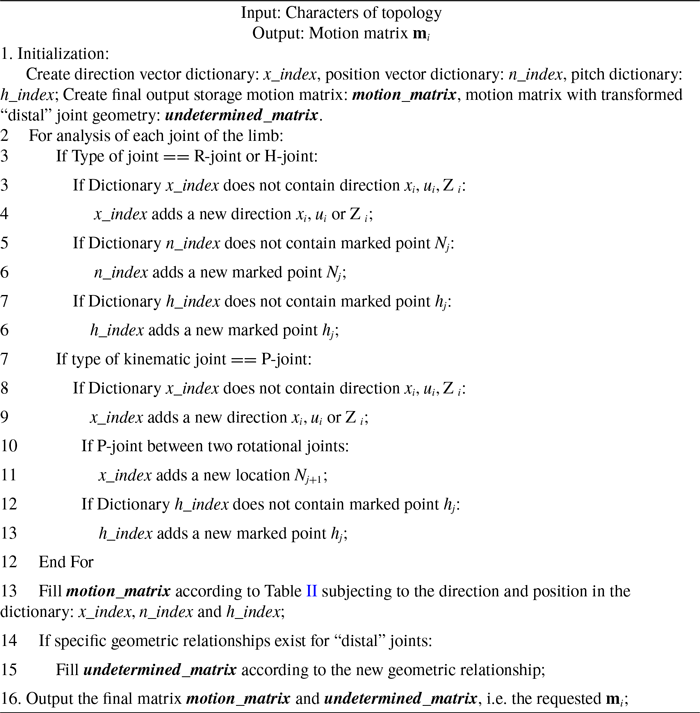
For example, submitting the topology character of Eq. (2a) into algorithm 1 as the input, the position and direction vectors of joints in each CRR limb could be inquired in dictionary. The motion matrix of 3-CRR mechanism could be obtained as
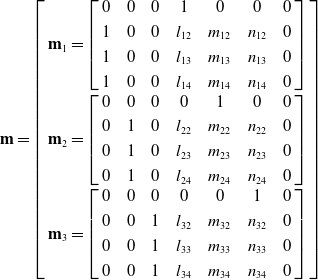 \begin{equation} \textbf{m}=\left[\begin{array}{l} \textbf{m}_{1}=\left[\begin{array}{c@{\quad}c@{\quad}c@{\quad}c@{\quad}c@{\quad}c@{\quad}c} 0 & 0 & 0 & 1 & 0 & 0 & 0\\[3pt] 1 & 0 & 0 & l_{12} & m_{12} & n_{12} & 0\\[3pt] 1 & 0 & 0 & l_{13} & m_{13} & n_{13} & 0\\[3pt] 1 & 0 & 0 & l_{14} & m_{14} & n_{14} & 0 \end{array}\right]\\[10pt] \textbf{m}_{2}=\left[\begin{array}{c@{\quad}c@{\quad}c@{\quad}c@{\quad}c@{\quad}c@{\quad}c} 0 & 0 & 0 & 0 & 1 & 0 & 0\\[3pt] 0 & 1 & 0 & l_{22} & m_{22} & n_{22} & 0\\[3pt] 0 & 1 & 0 & l_{23} & m_{23} & n_{23} & 0\\[3pt] 0 & 1 & 0 & l_{24} & m_{24} & n_{24} & 0 \end{array}\right]\\[10pt] \textbf{m}_{3}=\left[\begin{array}{c@{\quad}c@{\quad}c@{\quad}c@{\quad}c@{\quad}c@{\quad}c} 0 & 0 & 0 & 0 & 0 & 1 & 0\\[3pt] 0 & 0 & 1 & l_{32} & m_{32} & n_{32} & 0\\[3pt] 0 & 0 & 1 & l_{33} & m_{33} & n_{33} & 0\\[3pt] 0 & 0 & 1 & l_{34} & m_{34} & n_{34} & 0 \end{array}\right] \end{array}\right] \end{equation}
3. Predictive model of constraint/motion based on machine learning
In this section, a predictive model of constraints (motions) subjecting to the given motions (constraints) is constructed by machine learning. Not only numerical properties but also geometric conditions between motion and constraints are considered.
Constraints generated by component limbs would be obtained according to their motions:
where
![]() $\Gamma$
is the predictive model.
$\Gamma$
is the predictive model.
![]() $\textbf{m}_{i}$
and
$\textbf{m}_{i}$
and
![]() $\textbf{f}_{i}$
are the motion matrix of ith limb and its corresponding constraint matrix. It is noted that the constraints (motion) not only need to satisfy the reciprocity product with motion (constraint) but also expected to have the explicit meanings. To this end, machine learning is introduced to learn and reason the relationship between motion and constraints. Because motion and constraint have the dual solving process, the predictive model in Eq. (3a) could be also applied for motion solving when the constraints are known.
$\textbf{f}_{i}$
are the motion matrix of ith limb and its corresponding constraint matrix. It is noted that the constraints (motion) not only need to satisfy the reciprocity product with motion (constraint) but also expected to have the explicit meanings. To this end, machine learning is introduced to learn and reason the relationship between motion and constraints. Because motion and constraint have the dual solving process, the predictive model in Eq. (3a) could be also applied for motion solving when the constraints are known.
3.1. Equivalent motion transformation
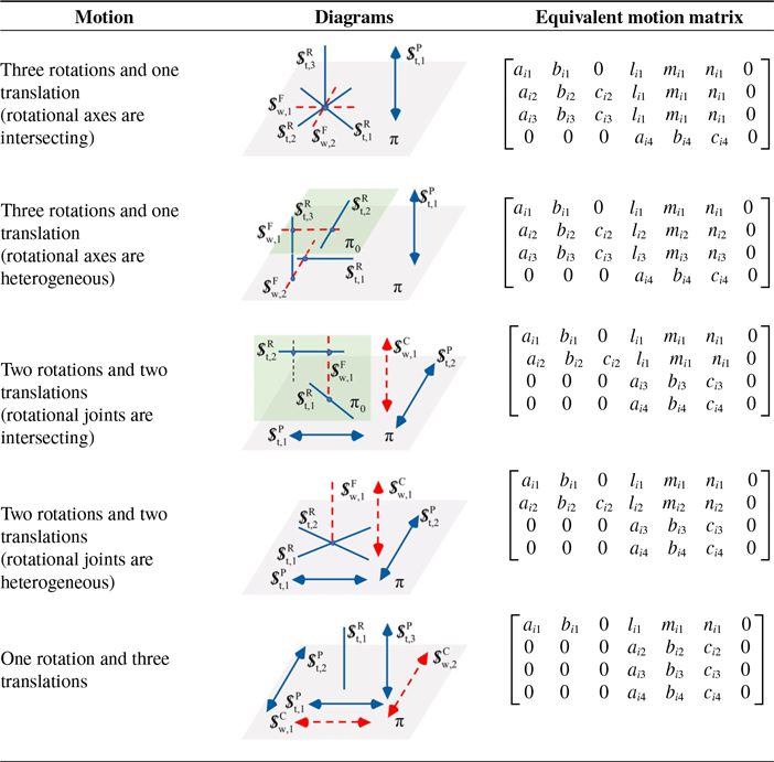
For some component limbs which contain rotational joints with parallel axes, the motion could be equivalently transformed firstly. For example, the motion matrix of the ith CRR limb could be described as Eq. (2d). It shows that the latter three rows are linear dependent, which could be equivalently transformed as
 \begin{equation} \textbf{m}_{i}=\left[\begin{array}{c@{\quad}c@{\quad}c@{\quad}c@{\quad}c@{\quad}c@{\quad}c} a_{i1} & b_{i1} & 0 & l_{i1} & m_{i1} & n_{i1} & 0\\[4pt] 0 & 0 & 0 & a_{i2} & b_{i2} & c_{i2} & 0\\[4pt] 0 & 0 & 0 & a_{i3} & b_{i3} & c_{i3} & 0\\[4pt] 0 & 0 & 0 & a_{i4} & b_{i4} & c_{i4} & 0 \end{array}\right] \end{equation}
Equation (3c) indicates that CRR limb has three translational motions and one rotational motion.
To simplify the inputs of machine learning network, the rotational motions with parallel axes would be transformed as translational motions preliminarily. It would not change the resultant constraints. Taking limbs with four-dimensional screws as example, the equivalent motion matrix is listed as Table III.
Table III. Equivalent motions of four-dimensional screws.
3.2. Optimal datasets with classification
To obtain the accurate constraints with explicit meanings, the geometric conditions between screw and its null space should be satisfied. Therefore, relative position and orientation characters are derived from motion matrix
![]() $\textbf{m}_{i}$
and taken as the input of machine learning network
$\textbf{m}_{i}$
and taken as the input of machine learning network
 \begin{equation} \textbf{input}=\left[\begin{array}{c@{\quad}c@{\quad}c@{\quad}c@{\quad}c} a_{1} & b_{1} & c_{1} & p_{1} & q_{1}\\ \vdots & \vdots & \vdots & \vdots & \vdots \\ a_{m} & b_{m} & c_{m} & p_{m} & q_{m} \end{array}\right] \end{equation}
where
![]() $m$
is the number of joints in the limb. Details of other variables are shown in Table IV.
$m$
is the number of joints in the limb. Details of other variables are shown in Table IV.
![]() $\boldsymbol{{s}}_{i}=(a_{i},b_{i},c_{i})$
and
$\boldsymbol{{s}}_{i}=(a_{i},b_{i},c_{i})$
and
![]() $p_{i}$
denote the orientation and position characters, respectively, which are classified by 14 and 7 types. It is defined that
$p_{i}$
denote the orientation and position characters, respectively, which are classified by 14 and 7 types. It is defined that
![]() $\boldsymbol{{s}}_{i}=(\begin{array}{lll} 1 & 0 & 0 \end{array})$
and
$\boldsymbol{{s}}_{i}=(\begin{array}{lll} 1 & 0 & 0 \end{array})$
and
![]() $\boldsymbol{{s}}_{i}=(\begin{array}{lll} 0 & 1 & 0 \end{array})$
indicate the parallel relationship between axis and basic platform and
$\boldsymbol{{s}}_{i}=(\begin{array}{lll} 0 & 1 & 0 \end{array})$
indicate the parallel relationship between axis and basic platform and
![]() $\boldsymbol{{s}}_{i}=(\begin{array}{lll} 0 & 0 & 1 \end{array})$
denotes the perpendicular relationship. When the vector is parallel with XY plane, two categories are defined as ±XY and +X-Y. Similarly, other kinds are shown in Table V. It is noted that when the direction is random,
$\boldsymbol{{s}}_{i}=(\begin{array}{lll} 0 & 0 & 1 \end{array})$
denotes the perpendicular relationship. When the vector is parallel with XY plane, two categories are defined as ±XY and +X-Y. Similarly, other kinds are shown in Table V. It is noted that when the direction is random,
![]() $\boldsymbol{{s}}_{i}=(\begin{array}{lll} 2 & 3 & 4 \end{array})$
is used. When
$\boldsymbol{{s}}_{i}=(\begin{array}{lll} 2 & 3 & 4 \end{array})$
is used. When
![]() $p_{i}=0$
, it denotes the arbitrary position relationship. When
$p_{i}=0$
, it denotes the arbitrary position relationship. When
![]() $p_{i}=\{1,\cdots,6\}$
, it denotes the order number of key points which can indicate the position.
$p_{i}=\{1,\cdots,6\}$
, it denotes the order number of key points which can indicate the position.
![]() $q_{i}$
is a sign to show the type of input, which is rotational motion (constraint force), translational motion (constraint couple), and screw motion (constraint screw).
$q_{i}$
is a sign to show the type of input, which is rotational motion (constraint force), translational motion (constraint couple), and screw motion (constraint screw).
Table IV. Definition of input and output of neural network.

Table V. Direction definition.

Table VI. Relationship between the direction vector and the axis of the joint.
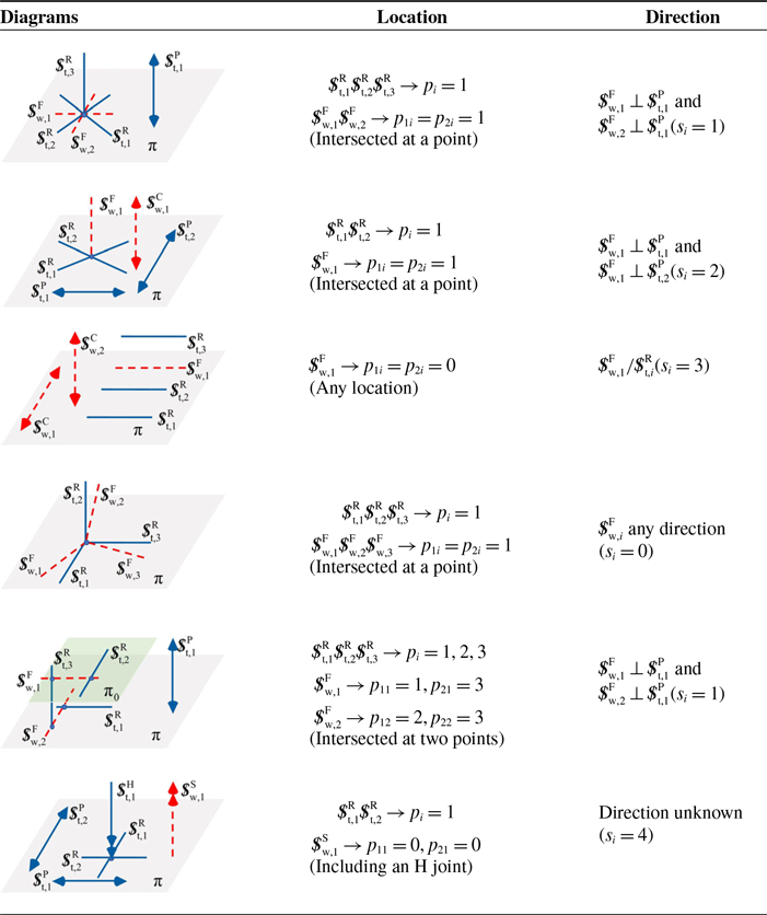
As shown in Table VI, the direction of reciprocal screw could be concluded as five groups: perpendicular with one screw axis, perpendicular with a plan spanning by two screw axes, parallel with one axis, arbitrary, and unknown. Herein, “arbitrary” denotes the force or couple constraint with alternative geometric conditions, and “unknown” indicates the case exists the motion or constraint screws, in which only numerical condition should be satisfied. The position of reciprocal screw is described by the intersection point with the given screws. In this way, the format of output is defined as
 \begin{equation} \textbf{output}=\left[\begin{array}{c@{\quad}c@{\quad}c@{\quad}c} s_{1} & p_{11} & p_{21} & q_{1}\\ \vdots & \vdots & \vdots & \vdots \\ s_{n} & p_{1n} & p_{2n} & q_{n} \end{array}\right] \end{equation}
where
![]() $s_{i}(s_{i}=0,1,\cdots,4)$
is defined as direction item as in Table V.
$s_{i}(s_{i}=0,1,\cdots,4)$
is defined as direction item as in Table V.
![]() $p_{1i}$
and
$p_{1i}$
and
![]() $p_{2i}$
denote the intersection points of rotational joints.
$p_{2i}$
denote the intersection points of rotational joints.
![]() $q_{i}$
has the same meaning as the input in Table IV.
$q_{i}$
has the same meaning as the input in Table IV.
Taking CRR limb as an example, the input matrix could be described as
 \begin{equation} \textbf{input}=\left[\begin{array}{c@{\quad}c@{\quad}c@{\quad}c@{\quad}c} 0 & 0 & 1 & 0 & -1\\ 0 & 0 & 1 & 1 & -2\\ 0 & 0 & 1 & 2 & -2\\ 0 & 0 & 1 & 3 & -2 \end{array}\right] \end{equation}
The output is given as
Another example is given as R ^ R ^ R-P limb; the input matrix could be described as
 \begin{equation} \textbf{input}=\left[\begin{array}{c@{\quad}c@{\quad}c@{\quad}c@{\quad}c} 2 & 3 & 4 & 1 & -2\\ 2 & 3 & 4 & 1 & -2\\ 2 & 3 & 4 & 1 & -2\\ 2 & 3 & 4 & 0 & -1 \end{array}\right] \end{equation}
where
![]() $d_{i}$
is random placeholder to expand the dataset and increase the generalization of the model. The output matrix is given as
$d_{i}$
is random placeholder to expand the dataset and increase the generalization of the model. The output matrix is given as
3.3. Neural network modeling
In this section, 5000 samples of motion and constraint matrix data are prepared and optimally classified as input and output, respectively. 80% of them are applied for training, and others are used in the test dataset. To achieve the mapping between motions and constraints, neural network (NN) for predictive model is formulated.
As shown in Fig. 1 (a), convolutional NN (CNN) is formulated, which consists of convolutional (Conv), flatten, hidden, and output layers. Conv layer performs element-by-element multiplication between input matrix and kernel of different weights. The weights are randomly generated at the beginning of the training. Following up flatten layer, data in vector form are transferred to the hidden layers, which contains two dense layers. Dense layer is responsible in encoding the features from previous layers in order to come up with relevant class and hence perform classification. In the output layer, constraint matrix would be returned to the model to compute the loss. Layer structure and parameters used in the considered CNN are listed in Table VII.
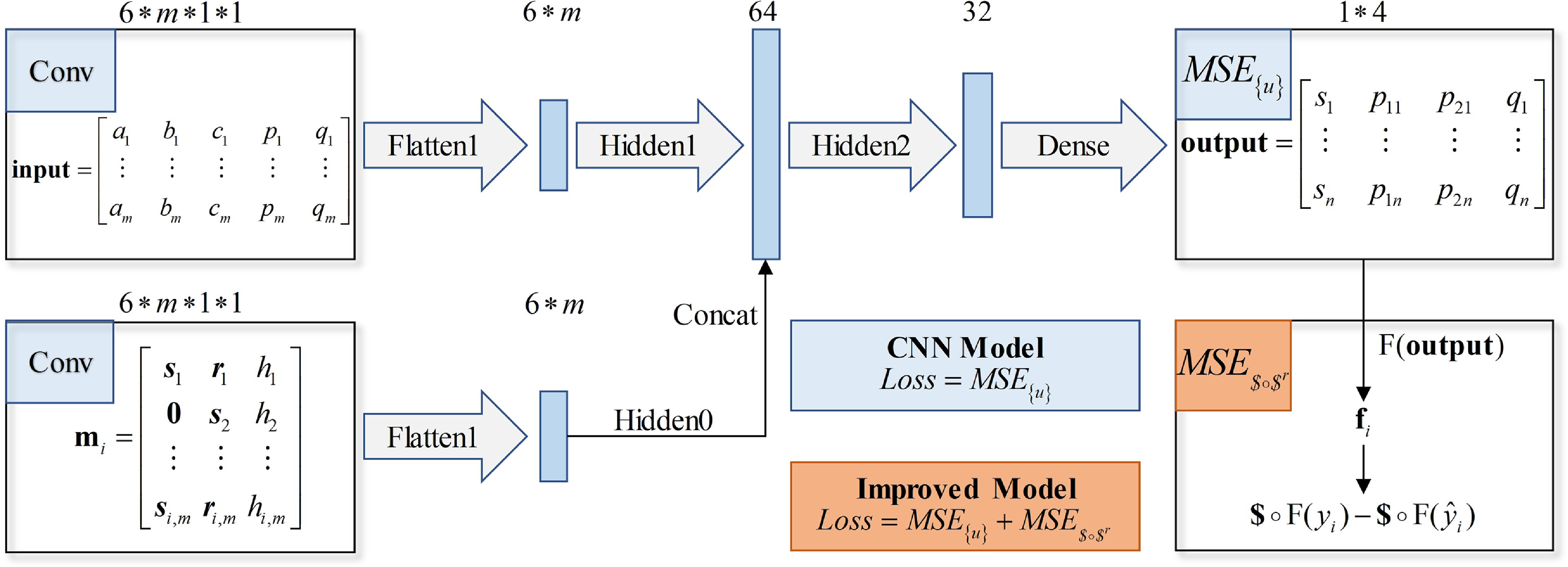
Figure 1. Architecture of CNN and improved model.
Table VII. Parameters of neural network.

The loss function of the CNN is defined as
where
![]() $n_{\textrm{s}}$
is the scale of the specimen.
$n_{\textrm{s}}$
is the scale of the specimen.
![]() $y_{i}$
and
$y_{i}$
and
![]() $\hat{y}_{i}$
are real value and prediction value of the model, respectively.
$\hat{y}_{i}$
are real value and prediction value of the model, respectively.
![]() $MSE_{\{u\}}$
is applied as mean-square error (
$MSE_{\{u\}}$
is applied as mean-square error (
![]() $\textrm{MSE}$
) of network.
$\textrm{MSE}$
) of network.
![]() $SSE$
denotes the sum of squares due to error.
$SSE$
denotes the sum of squares due to error.
![]() $w_{mse1}$
is the weight of
$w_{mse1}$
is the weight of
![]() $MSE_{\{u\}}$
in loss function, where
$MSE_{\{u\}}$
in loss function, where
![]() $w_{mse1}=1$
.
$w_{mse1}=1$
.
When taking partial derivative of network weight w
0 of on both sides of
![]() $MSE_{\{u\}}$
, the descending gradient goes toward the fewer error of network. The loss and Pearson correlation coefficient between the real and prediction outputs are illustrated in Fig. 2 (a), resulting in the accuracy of prediction model.
$MSE_{\{u\}}$
, the descending gradient goes toward the fewer error of network. The loss and Pearson correlation coefficient between the real and prediction outputs are illustrated in Fig. 2 (a), resulting in the accuracy of prediction model.
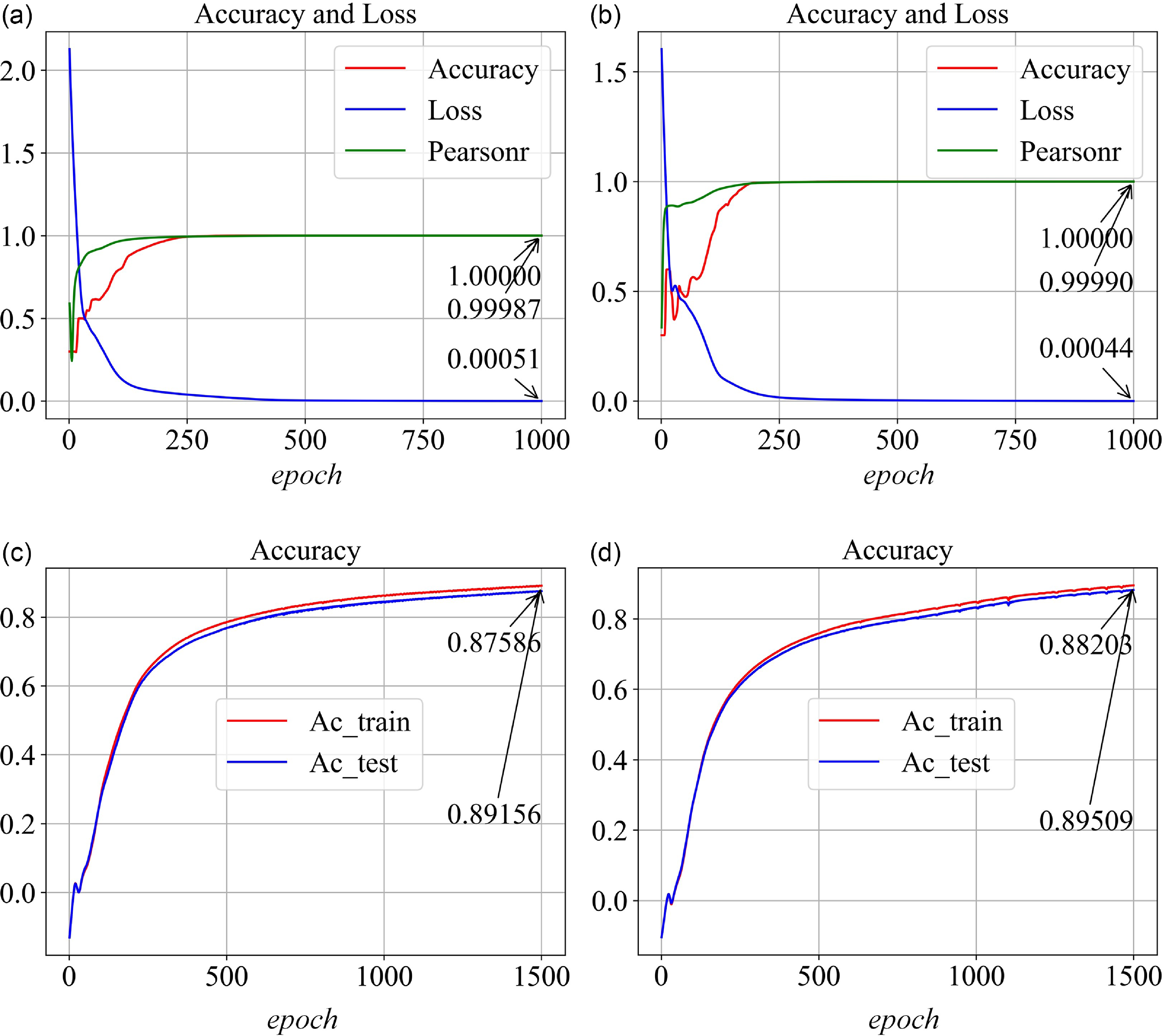
Figure 2. Performance comparison of CNN and improved model. (a) Accuracy and loss of output matrix of CNN model. (b) Accuracy and loss of output matrix of improved model. (c) Accuracy of motion/constraint prediction of CNN model. (d) Accuracy of motion/constraint prediction of CNN model.
It is noted that reciprocal screws should satisfy the numerical relationship as accurate as possible. Therefore, a physic constraint is introduced as
where
![]() $MSE_{{^{\boldsymbol{{\$}} \circ {\boldsymbol{{\$}} ^{r}}}}}$
indicates the mean-square error of reciprocal product.
$MSE_{{^{\boldsymbol{{\$}} \circ {\boldsymbol{{\$}} ^{r}}}}}$
indicates the mean-square error of reciprocal product.
![]() $w_{mse2}$
is the weight where
$w_{mse2}$
is the weight where
![]() $w_{mse2}=0.001*\textit{epoch}$
, and epoch is the iteration. “
$w_{mse2}=0.001*\textit{epoch}$
, and epoch is the iteration. “
![]() $\circ$
” denotes the reciprocal product between the twist
$\circ$
” denotes the reciprocal product between the twist
![]() $\boldsymbol{{\$}}_{\textrm{t},i}$
of the ith motion derived from motion matrix and the real constraint wrench
$\boldsymbol{{\$}}_{\textrm{t},i}$
of the ith motion derived from motion matrix and the real constraint wrench
![]() $\textrm{F}(y_{i})$
(the predictive constraint wrench
$\textrm{F}(y_{i})$
(the predictive constraint wrench
![]() $\textrm{F}(\hat{y}_{i})$
). Therefore, the compressive and real-time loss function is proposed as
$\textrm{F}(\hat{y}_{i})$
). Therefore, the compressive and real-time loss function is proposed as
To this end, a novel network is formulated as Improved Neural Network by Algorithm 2. The architecture of the network is the same with CNN in terms of the convolutional layers used. Besides the loss of model considered in CNN, the novel network also learns the physic principle as reciprocity between motion and constraint, which can improve the generalization of the predictive model. The performance of new model is depicted in Fig. 2 (b), which decreases the loss as small as 0.044%. When applying the prediction model on training and test sets, the probability to get accurate motion/constraint is presented in Fig. 2 (c) and (d), respectively. It shows that the improved model has a better accuracy as high as 89.5% for a new issue.
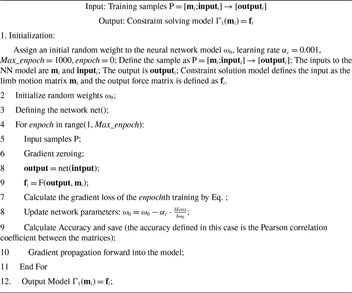
Algorithm 2: Neural network-based constraint solving model
It shows that improved model could reach higher accuracy. To find out the reason,
![]() $MSE_{\boldsymbol{{\$}} \circ {\boldsymbol{{\$}} ^{r}}}$
computed from both CNN and improved model are also compared in Fig. 3. It is recorded that improved model has the better performance in the loss of reciprocal product, resulting from the loss function with physical equation. Although the difference would be decreased following with training generations, the former model is prior than the latter one as 30% after iterative 1000.
$MSE_{\boldsymbol{{\$}} \circ {\boldsymbol{{\$}} ^{r}}}$
computed from both CNN and improved model are also compared in Fig. 3. It is recorded that improved model has the better performance in the loss of reciprocal product, resulting from the loss function with physical equation. Although the difference would be decreased following with training generations, the former model is prior than the latter one as 30% after iterative 1000.
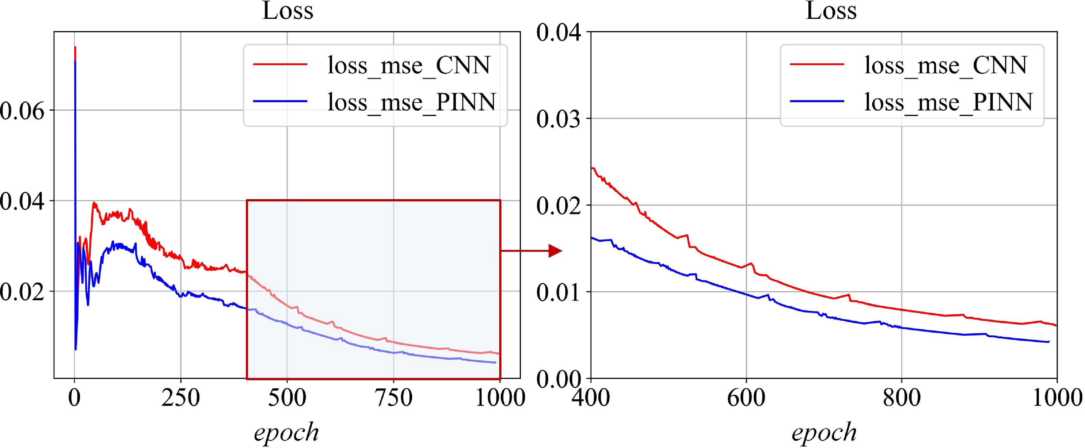
Figure 3.
![]() $MSE_{\boldsymbol{{\$}} \circ {\boldsymbol{{\$}} ^{r}}}$
comparison of improved model and CNN.
$MSE_{\boldsymbol{{\$}} \circ {\boldsymbol{{\$}} ^{r}}}$
comparison of improved model and CNN.
Therefore, improved model is applied for predictive modeling. In fact, from the view of meaningful motion and constraint, both the errors of numerical and geometric features should be considered; that is why improved model has better performance in this case.
4. Application in automatic mobility analysis
Applying the reciprocal screw solving method, the procedure to identify the mobility of parallel mechanisms could be proposed by four steps as shown Fig. 4:
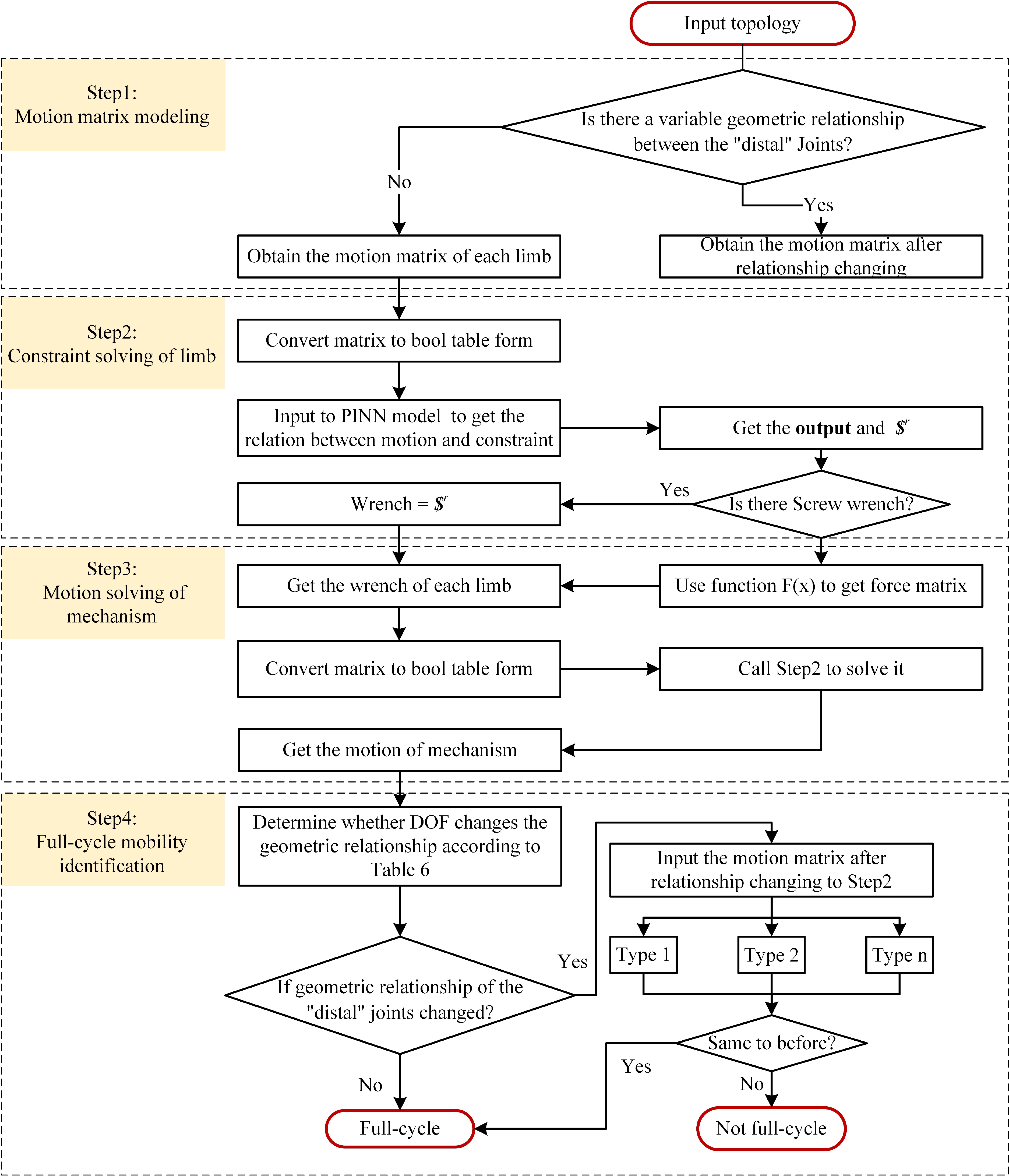
Figure 4. Flowchart of mobility analysis of parallel mechanisms.
Step 1: Having topology character at hand, motion matrix would be obtained automatically by Algorithm 1. It would be identified that whether there exist distal joints. If so, the relationship after changing would also be constructed.
Step 2: The motion matrix from step 1 is transformed as boolean matrix, which is the input of improved predictive model. The constraints of all limbs are obtained in the format of boolean matrix as output.
Step 3: The independent constraints in boolean matrix format are given to the improved predictive model. The motion of moving platform is derived and transformed as DoF matrix.
 \begin{equation} \textbf{DoF}=\left[\begin{array}{c@{\quad}c@{\quad}c} \boldsymbol{{s}}_{1} & \boldsymbol{{r}}_{1} & h_{1}\\ \vdots & \vdots & \vdots \\ \boldsymbol{{s}}_{n} & \boldsymbol{{r}}_{n} & h_{n} \end{array}\right]_{n\ast 7} \end{equation}
Taking 3-CRR mechanism as an example, the DoF matrix would be obtained as
 \begin{equation} \textbf{DoF}=\left[\begin{array}{c@{\quad}c@{\quad}c@{\quad}c@{\quad}c@{\quad}c@{\quad}c} 0 & 0 & 0 & 1 & 0 & 0 & 0\\[4pt] 0 & 0 & 0 & 0 & 1 & 0 & 0\\[4pt] 0 & 0 & 0 & 0 & 0 & 1 & 0 \end{array}\right] \end{equation}
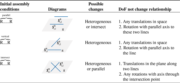
Step 4: For the mechanism exists distal joints, the full-cycle motion is distinguished. For example, the first and last rotational joints of UPU limb are considered as distal joints. When the second and the fourth joints have parallel motion axes and complementary motion, the geometry condition of distal joints would not be changed in the movement. But in the other case, the motion axes of distal joints would change to be intersecting or in different flats. At this moment, the motion and constraints would be changed. The mobility analysis should be considered separately. The situations for distal joints without changing mobility and constraints are concluded in Table VIII.
Table VIII. Identification of distal joints.
5. Software implementation
By integrating the algorithms and models with Python 3.7 programming language, a software is developed under B/S framework supporting automatic and visualized procedure for motion and constraint analysis of parallel mechanisms. Three interactive windows are designed as input of topology, output of mobility analysis, and visualization of constraints as shown in Fig. 5.
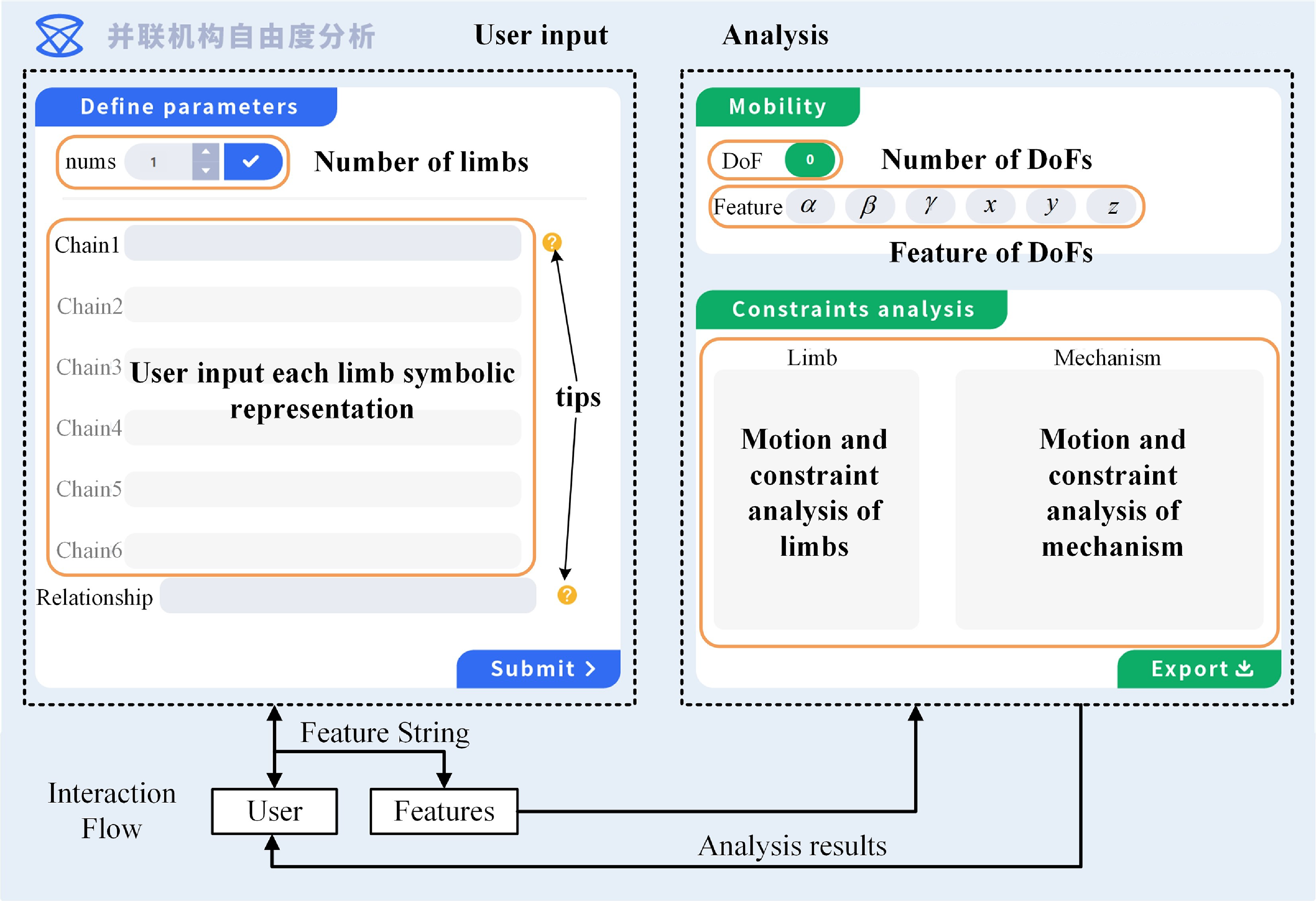
Figure 5. Module of web platform.
-
1. Input of topology
This window allows users to input the required topology characters, which is located on the right of the interactive interface. Users would give the number of limbs firstly followed with the topology characters of each limb. If someone needs help, he can find out the rules in tips “?”. Thanks to Algorithm 1, topology characters would be identified by the software, which would be transformed as motion matrix to the next step.
-
2. Visualization of constraints
This module illustrates the motion axes and constraints of limbs and moving platform with lines, points, and other geometric elements. The types of geometric elements are defined and associated with different motion and constraints thanks to WebGL interface. A drawer engine is programmed. Firstly, the framework assigned as O-xyz is constructed on the canvas. When the topology is given and motion matrix is solved, the first joint of one limb is located at a fixed point and along x-axis, which is taken as a reference. Other joints and limbs are illustrated according to the motion matrix with positions determined by the marked points and directions selected by
![]() $\boldsymbol{{s}}_{i}$
. The constraints would be drawn thanks to the geometric conditions involved in input and output matrix. The lines of different meanings are applied by matplotlib three-dimensional, which is a graphic library of Python.
$\boldsymbol{{s}}_{i}$
. The constraints would be drawn thanks to the geometric conditions involved in input and output matrix. The lines of different meanings are applied by matplotlib three-dimensional, which is a graphic library of Python.
-
3. Output of mobility analysis
Once the topology characters are provided, the user accesses the mobility including the number and type of motions. The results are provided to users by concise alternatives on the right side. Here, NN for null space of screw system solving plays key roles for this function.
The software could be implemented by the following steps:
-
1. Input the topology characters such as the number and types of limbs into the software.
-
2. Motion matrix of each limb is obtained by Algorithm 1 and equivalent transformed to be
 $\textbf{m}_{i}$
.
 -
3. Taking
 $\textbf{m}_{i}$
as the input of model
 $\Gamma (\textbf{m}_{i})=\textbf{f}_{i}$
, constraint matrix of each branch would be obtained as.
 -
4. Taking
 $\textbf{f}=[\textbf{f}_{1},\cdots,\textbf{f}_{n}]$
as the input of model
 $\Gamma (\textbf{f})=\textbf{m}$
, motion matrix of moving platform would be obtained as
 $\textbf{m}$
.
 -
5. Special geometric relationship as “distal” kinematic joints would be determined based on Table VIII. If so, steps (3) and (4) are repeated.
-
6. Input
 $\textbf{m}_{i}, \textbf{f}_{i}, \textbf{m}, \textbf{f}$
to WebGL drawer engine.
 -
7. Output the results of mobility and constraints to users.
6. Cases study and discussion
6.1. 3-CRR mechanism
The motion and constraints analysis of 3-CRR has been addressed above, which is not introduced here again. When topology character as in Eq. (2a) is entered the into the software, the result could be obtained as in Fig. 6.

Figure 6. Motion and constraint analysis result of 3-CRR mechanism.
It is concluded that each limb of 3-CRR mechanism has two constraint couples, which are perpendicular with the motion axes of R joint. The moving platform of mechanism undergoes three constraint couples, resulting in three translational motions, which is a full-cycle mobility.
6.2. 3-UPU mechanism
3-UPU is a typical parallel mechanism with different assembly conditions and alternative mobilities. It is assumed that the motion axes of 1st and 5th rotational joints are parallel at initial state, which constitute as “distal” joints. However, not only assembly conditions in the same limb but also among different limbs would affect the motion and constraints of parallel mechanism. Here, two cases are discussed to verify the method:
(a) Three UPU limbs are symmetrically assembled.
In this case, three limbs are symmetrically assembled with non-parallel plane of U joint. The topology characters should be given as
 \begin{equation} \left\{\begin{array}{c} x_{1}N_{1}\textrm{R}N_{1}\,|\,u_{1}N_{1}\textrm{R}N_{1}\,|\,N_{1}N_{2}\textrm{P}\,|\,u_{1}N_{2}\textrm{R}N_{2}\,|\,x_{1}N_{2}\textrm{R}N_{2}\\[4pt] x_{2}N_{3}\textrm{R}N_{3}\,|\,u_{2}N_{3}\textrm{R}N_{3}\,|\,N_{3}N_{4}\textrm{P}\,|\,u_{2}N_{4}\textrm{R}N_{4}\,|\,x_{2}N_{4}\textrm{R}N_{4}\\[4pt] x_{3}N_{5}\textrm{R}N_{5}\,|\,u_{3}N_{5}\textrm{R}N_{5}\,|\,N_{5}N_{6}\textrm{P}\,|\,u_{3}N_{6}\textrm{R}N_{6}\,|\,x_{3}N_{6}\textrm{R}N_{6} \end{array}\right\} \end{equation}
The motion matrix of limb is solved as
 \begin{equation} \textbf{m}_{i}=\left[\begin{array}{c@{\quad}c@{\quad}c@{\quad}c@{\quad}c@{\quad}c} a_{i1} & b_{i1} & 0 & l_{i1} & m_{i1} & n_{i1}\\ a_{i2} & b_{i2} & c_{i2} & l_{i1} & m_{i1} & n_{i1}\\ 0 & 0 & 0 & l_{i3}-l_{i1} & m_{i3}-m_{i1} & n_{i3}-n_{i1}\\ a_{i2} & b_{i2} & c_{i2} & l_{i3} & m_{i3} & n_{i3}\\ a_{i1} & b_{i1} & 0 & l_{i3} & m_{i3} & n_{i3} \end{array}\right] \end{equation}
The motion matrix of the ith limb lies in the format as
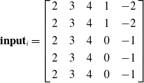 \begin{equation} \textbf{inpu}\textbf{t}_{i}=\left[\begin{array}{c@{\quad}c@{\quad}c@{\quad}c@{\quad}c} 2 & 3 & 4 & 1 & -2\\[3pt] 2 & 3 & 4 & 1 & -2\\[3pt] 2 & 3 & 4 & 0 & -1\\[3pt] 2 & 3 & 4 & 0 & -1\\[3pt] 2 & 3 & 4 & 0 & -1 \end{array}\right] \end{equation}
As illustrated in Fig. 7, each UPU limb provides a couple constraint, which is perpendicular to its plane of U joint. The moving platform has three independent couples, leading to the matrix for DoF
 \begin{equation} \textbf{DoF}=\left[\begin{array}{c@{\quad}c@{\quad}c@{\quad}c@{\quad}c@{\quad}c@{\quad}c} 0 & 0 & 0 & 1 & 0 & 0 & 0\\[4pt] 0 & 0 & 0 & 0 & 1 & 0 & 0\\[4pt] 0 & 0 & 0 & 0 & 0 & 1 & 0 \end{array}\right] \end{equation}

Figure 7. Motion and constraint analysis result of 3-UPU mechanism with symmetric structure.
It indicates that 3-UPU with fully symmetric topology has three translational motions. The “distal” joints are falling in situation (a) listed in Table VIII, which would not change the constraints and further the mobility. Therefore, 3-UPU has a full-cycle three-dimensional translational motion [Reference Zhao, Chen, Li and Huang25].
(b) Motion axes of first joint of three limbs are parallel.
In this case, the planes of U joint of limbs are parallel with each other. The input would be
 \begin{equation} \left\{\begin{array}{c} x_{1}N_{1}\textrm{R}N_{1}\,|\,x_{2}N_{1}\textrm{R}N_{1}\,|\,N_{1}N_{2}P\,|\,x_{2}N_{2}\textrm{R}N_{2}\,|\,x_{1}N_{2}\textrm{R}N_{2}\\[4pt] x_{1}N_{3}\textrm{R}N_{3}\,|\,x_{2}N_{3}\textrm{R}N_{3}\,|\,N_{1}N_{2}P\,|\,x_{2}N_{4}\textrm{R}N_{4}\,|\,x_{1}N_{4}\textrm{R}N_{4}\\[4pt] x_{1}N_{5}\textrm{R}N_{5}\,|\,x_{2}N_{5}\textrm{R}N_{5}\,|\,N_{1}N_{2}P\,|\,x_{2}N_{6}\textrm{R}N_{6}\,|\,x_{1}N_{6}\textrm{R}N_{6} \end{array}\right\} \end{equation}
Motion matrix of limb is formulated easily as
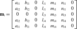 \begin{equation} \textbf{m}_{i}=\left[\begin{array}{c@{\quad}c@{\quad}c@{\quad}c@{\quad}c@{\quad}c@{\quad}c} a_{i1} & b_{i1} & 0 & l_{i1} & m_{i1} & n_{i1} & 0\\ a_{i2} & b_{i2} & 0 & l_{i1} & m_{i1} & n_{i1} & 0\\ 0 & 0 & 0 & l_{i3} & m_{i3} & n_{i3} & 0\\ a_{i2} & b_{i2} & 0 & l_{i4} & m_{i4} & n_{i4} & 0\\ a_{i1} & b_{i1} & 0 & l_{i4} & m_{i4} & n_{i4} & 0 \end{array}\right] \end{equation}
The output indicates a couple
It is noted that each limb provides a same couple. In this moment, the DoF matrix would be
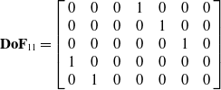 \begin{equation} \textbf{Do}\textbf{F}_{11}=\left[\begin{array}{c@{\quad}c@{\quad}c@{\quad}c@{\quad}c@{\quad}c@{\quad}c} 0 & 0 & 0 & 1 & 0 & 0 & 0\\ 0 & 0 & 0 & 0 & 1 & 0 & 0\\ 0 & 0 & 0 & 0 & 0 & 1 & 0\\ 1 & 0 & 0 & 0 & 0 & 0 & 0\\ 0 & 1 & 0 & 0 & 0 & 0 & 0 \end{array}\right] \end{equation}
which indicates two rotational and three translational motions. There exist “distal” joints, but out of the scope without changing, it will affect the constraints and mobility. Therefore, the mobility indicated in Eq. (6e) is not full cycle, in which case the software would inform users by a popup as in Fig. 8 (a).

Figure 8. Motion and constraint analysis result of 3-UPU mechanism with parallel axes.
The motion matrix would be changed as
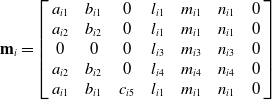 \begin{equation} \textbf{m}_{i}=\left[\begin{array}{c@{\quad}c@{\quad}c@{\quad}c@{\quad}c@{\quad}c@{\quad}c} a_{i1} & b_{i1} & 0 & l_{i1} & m_{i1} & n_{i1} & 0\\ a_{i2} & b_{i2} & 0 & l_{i1} & m_{i1} & n_{i1} & 0\\ 0 & 0 & 0 & l_{i3} & m_{i3} & n_{i3} & 0\\ a_{i2} & b_{i2} & 0 & l_{i4} & m_{i4} & n_{i4} & 0\\ a_{i1} & b_{i1} & c_{i5} & l_{i1} & m_{i1} & n_{i1} & 0 \end{array}\right] \end{equation}
The output of constraint from the ith limb is written as
which indicates a constraint force. In this moment, the DoF matrix would be
 \begin{equation} \textbf{DoF}=\left[\begin{array}{c@{\quad}c@{\quad}c@{\quad}c@{\quad}c@{\quad}c@{\quad}c} 1 & 0 & 0 & 0 & 0 & 0 & 0\\ 0 & 1 & 0 & 0 & 0 & 0 & 0\\ 0 & 0 & 0 & 1 & 0 & 0 & 0\\ 0 & 0 & 0 & 0 & 0 & 1 & 0 \end{array}\right] \end{equation}
which indicates two rotational and two translational motions, as illustrated in Fig. 8 (b).
Compared with case (a), it could be seen that the arrangement of limbs would affect the resultant mobility. It is necessary to observe the constraints in the process. In this situation, the mobility at initial pose is considered as non-full cycle DoF, which would be changed once there is a rotational movement between the 1st and the last joints. The software depicts this phenomenon and shows it to users by a window. When the motion axes have been changed, it falls in the four DoF, which is a full-cycle mobility which is illustrated in the main page. From this point, the initial pose could be considered as a singular pose of the mechanism. In this way, the software can provide much information to users rather than the mobility.
6.3. Exechon robot
Exechon robot is famous in machining, which is composed of two UPR limbs and one SPR limb. The topology could be characterized as
 \begin{equation} \left\{\begin{array}{c} x_{1}N_{1}\textrm{R}N_{1}\,|\,x_{2}N_{1}\textrm{R}N_{1}\,|\,N_{1}N_{2}\textrm{P}\,|\,x_{2}N_{2}\textrm{R}N_{2}\\[4pt] x_{1}N_{1}\textrm{R}N_{1}\,|\,x_{2}N_{1}\textrm{R}N_{1}\,|\,N_{1}N_{2}\textrm{P}\,|\,x_{2}N_{2}\textrm{R}N_{2}\\[4pt] u_{1}N_{4}\textrm{R}N_{4}\,|\,u_{2}N_{4}\textrm{R}N_{4}\,|\,u_{3}N_{4}\textrm{R}N_{4}\,|\,N_{4}N_{5}\textrm{P}\,|\,x_{3}N_{5}\textrm{R}N_{5} \end{array}\right\} \end{equation}
Based on the algorithms and predictive model, the result of mobility and constraint analysis is generated by the software as shown in Fig. 9, which is consistent with the result in ref. [Reference Hu26].
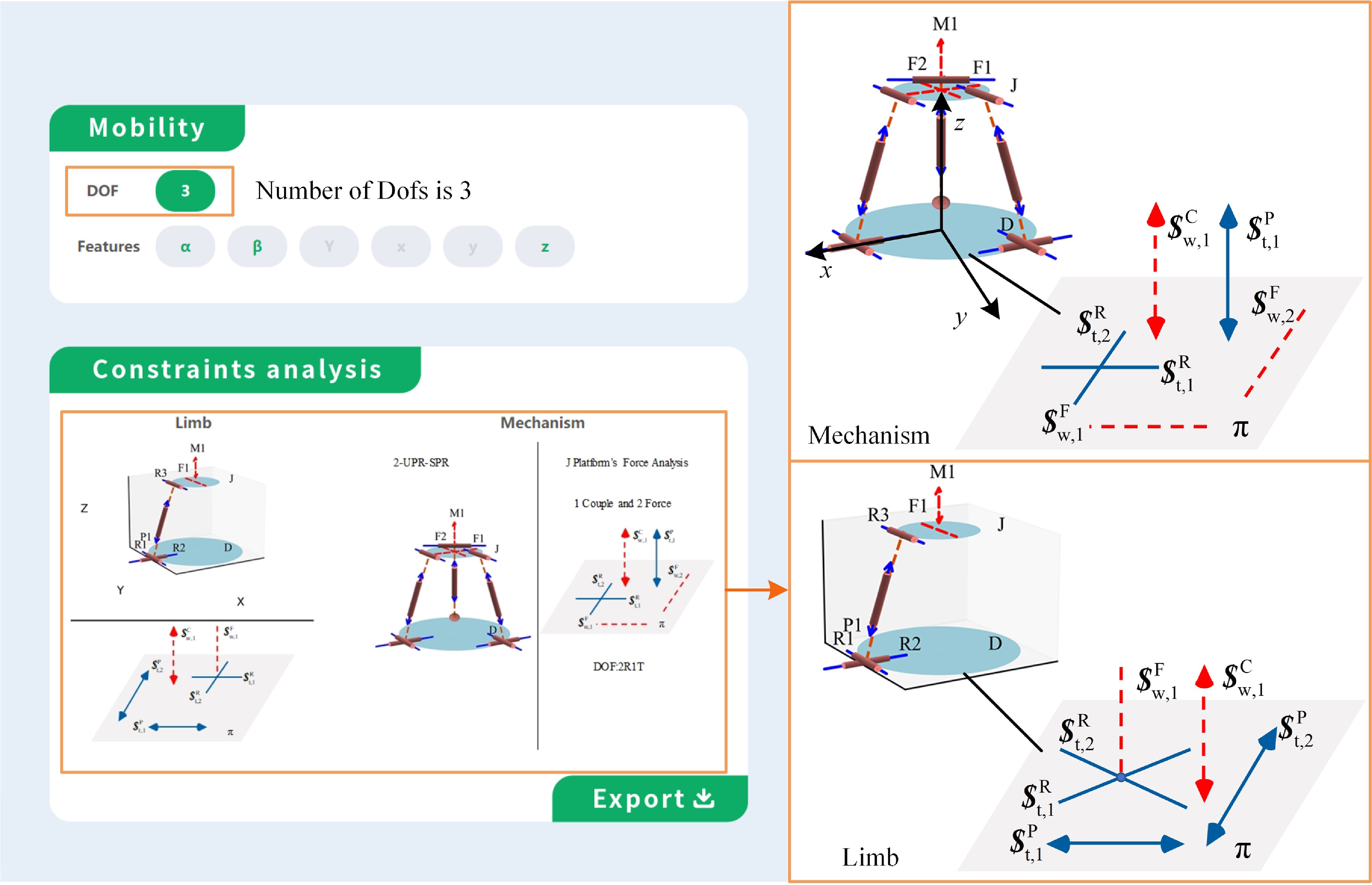
Figure 9. Motion and constraint analysis result of exechon mechanism.
It could be seen from the visual constraints that UPR limb provides one couple and one force constraints, and SPR limb provides one force constraints. It is a redundant mechanism which has two couples and three forces. Among them, one couple and two forces are independent. Therefore, the mechanism has two rotational motions and one translational motion. The detail process is given in appendix.
6.4. Omni III robot
Omni III robot is composed of four RRRR limbs. The first joints of limbs are perpendicular with each other, and the adjacent two joints are intersected at one point. The input could be given as
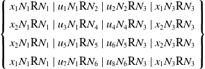 \begin{equation} \left\{\begin{array}{c} x_{1}N_{1}\textrm{R}N_{1}\,|\,u_{1}N_{1}\textrm{R}N_{2}\,|\,u_{2}N_{2}\textrm{R}N_{3}\,|\,x_{1}N_{3}\textrm{R}N_{3}\\[4pt] x_{2}N_{1}\textrm{R}N_{1}\,|\,u_{3}N_{1}\textrm{R}N_{4}\,|\,u_{4}N_{4}\textrm{R}N_{3}\,|\,x_{2}N_{3}\textrm{R}N_{3}\\[4pt] x_{2}N_{1}\textrm{R}N_{1}\,|\,u_{5}N_{1}\textrm{R}N_{5}\,|\,u_{6}N_{5}\textrm{R}N_{3}\,|\,x_{2}N_{3}\textrm{R}N_{3}\\[4pt] x_{1}N_{1}\textrm{R}N_{1}\,|\,u_{7}N_{1}\textrm{R}N_{6}\,|\,u_{8}N_{6}\textrm{R}N_{3}\,|\,x_{1}N_{3}\textrm{R}N_{3} \end{array}\right\} \end{equation}
Based on the algorithms and predictive model, the result of mobility and constraint analysis is generated by the software as shown in Fig. 10, which is consistent with the result in ref. [Reference Chang-Siu, Snell, McInroe, Balladarez and Full27].

Figure 10. Motion and constraint analysis result of Omni III robot.
It could be seen from the visual constraints that each RRRR limb provides two force constraints in the plane
![]() $\pi$
. It is a redundant mechanism which has eight forces. Among them, three forces and one couple are independent. Therefore, the mechanism has two rotational motions, which can move as a simi-sphere and is famous as simi-sphere mechanism. The detail process is given in appendix.
$\pi$
. It is a redundant mechanism which has eight forces. Among them, three forces and one couple are independent. Therefore, the mechanism has two rotational motions, which can move as a simi-sphere and is famous as simi-sphere mechanism. The detail process is given in appendix.
6.5. 2-PPPHR mechanism
2-PPPHR mechanism is composed of two PPPHR limbs. The first joints of limbs are perpendicular with each other, and the adjacent two joints are intersected at one point. The input could be given as
 \begin{equation} \left\{\begin{array}{c} z_{1}z_{1}\textrm{P}\,|\,x_{1}x_{1}\textrm{P}\,|\,x_{2}x_{2}\textrm{P}\,|\,x_{2}N_{1}\textrm{H}N_{1}\,|\,x_{3}N_{2}\textrm{R}N_{2}\\[4pt] z_{1}z_{1}\textrm{P}\,|\,x_{1}x_{1}\textrm{P}\,|\,x_{2}x_{2}\textrm{P}\,|\,x_{2}N_{3}\textrm{H}N_{3}\,|\,x_{3}N_{4}\textrm{R}N_{4} \end{array}\right\} \end{equation}
Based on the algorithms and predictive model, the result of mobility and constraint analysis is generated by the software as shown in Fig. 11, which is consistent with the result in ref. [Reference Li, Wu, Shen, Muller, Liu and Yang22].
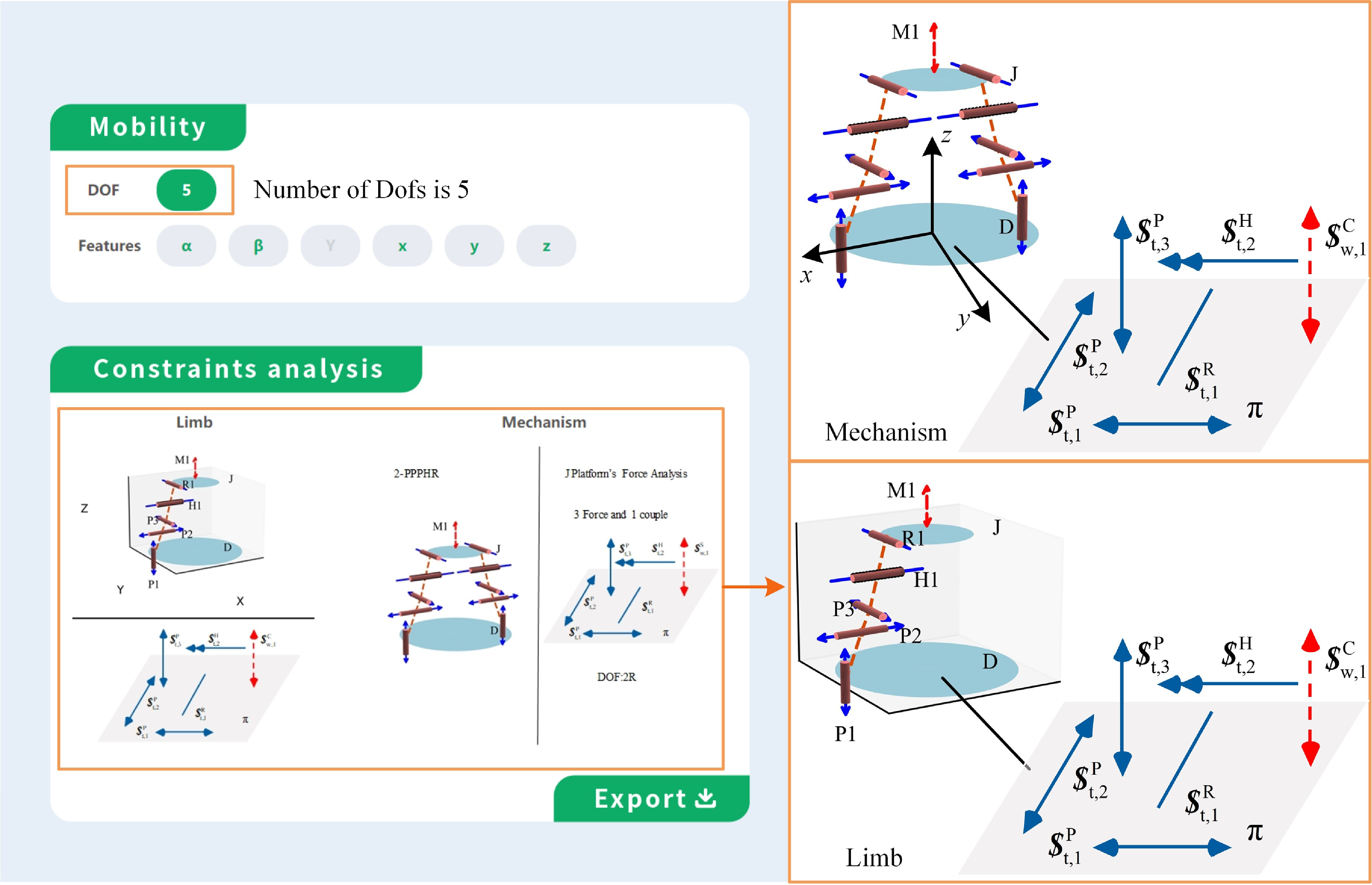
Figure 11. Motion and constraint analysis result of 2-PPPHR.
It could be seen from the visual constraints that the two PPPHR limbs provide a same couple constraint. Therefore, the mechanism has two rotational and three translational motions. The detail process is given in appendix.
6.6. Discussion
As a preliminary step, twist and wrench should be solved in a concise and efficient manner. To achieve this, two primary methods have been developed: numerical computation and observation of null-space.
For the numerical method, alternative solutions could be obtained when the number of equations is less than five. These solutions satisfy the algebraic relationship but are failing with the geometric features. For example, the constraints of limbs in cases 6.1–6.4 would have multi-solutions by solving null-space. In contrast, the predictive approach applies artificial intelligence to learn the geometric features of reciprocal screws, which are granted the real meanings.
For the observation method, it requires extensive human knowledge, which is hard to be programmed and handle with the amount of cases. Furthermore, when there exist helical joints in the screw system, observation method would not be comfortable anymore. Besides geometric features, the predictive approach also takes algebraic properties as loss function, which can improve the accuracy and solve the case with helical joint like case 6.5.
As a universal function fitter, NN has become another way to solve the above problems. A single perceptron can simulate three operations: AND, OR, and NOT. Three perceptrons forming a perceptron network including one hidden layer can simulate all operations. Therefore, NNs can simulate any combination of logical functions in theory. Specifically, this ability is mainly based on the following aspects:
-
1. Machine learning can identify complex patterns and rules from data, including relationships between inputs and outputs. These patterns and rules can be abstracted into the “IF…THEN…”-type conditional statements.
-
2. Machine learning constructs models by learning and training on datasets, rather than relying on manually crafted rules. This allows machine learning to automatically extract features and patterns from data.
-
3. Once the patterns and rules are learned from data, the machine learning typically generalizes this knowledge to previously unseen data. This means that even when dealing with new situations or data, the model can make accurate predictions or decisions.
Using the powerful fitting capabilities of machine learning, the results obtained from this approach would be consistent with those of manual observation and numerical computation, and the advantages of the proposed automated method are summarized in Table IX.
Table IX. Comparison with existing theoretical analysis methods.

7. Conclusions
This paper investigates the automatic identification method for motion/constraint and mobility of parallel mechanisms based on machine learning. The following conclusions could be drawn:
-
1. Topology is characterized by symbols, including the type of limbs with the direction and position of motion axis relative to fixed platform. Motion matrix is defined by signing key points. The mapping between topology and motion is formulated by algorithm.
-
2. Predictive model for reciprocal screw is constructed by NN, which reaches 89.5% accuracy by defining a physical-informed loss function. In this way, motion and constraints are solved with natural meanings and numerical properties.
-
3. Automatic mobility analysis procedure is proposed by four steps based on the predictive model. Full-cycle mobility is identified considering the “distal” joints.
-
4. The online software for visualization constraint and mobility analysis is developed, and five typical examples are given.
The automatic approach proposed in this article not only provides the results from mobility analysis but also gives an insight investigation of meaningful motion and constraints. It offers additional benefits by providing clear visual information and aiding in kinematic modeling, including singularity analysis. In our future work, time series data structures for finite motion description would be well investigated. Additionally, we aim to integrate topology synthesis, analysis, and design visually and intelligently, taking into account both the characteristics of finite motion and constraints.
Author contributions
Huo and Song constructed the machine learning model. Sun developed the demo and wrote the article.
Financial support
This research work was supported by the National Natural Science Foundation of China (NSFC) under Grant No. 52205028, No. 62027812 and No. 52275027, and Tianjin Research Program of Technology under Grant No. 20201193 and No. 22JCZDJC00350.
Competing interests
The authors declare no competing interests.
Ethical approval
None.
Appendix
-
a. Exechon robot
(1) Step 1: motion matrix could be
 \begin{equation} \textbf{m}=\left[\begin{array}{c} \textbf{m}_{1}=\left[\begin{array}{c@{\quad}c@{\quad}c@{\quad}c@{\quad}c@{\quad}c} 1 & 0 & 0 & l_{11} & m_{11} & n_{11}\\[5pt] 0 & 1 & 0 & l_{11} & m_{11} & n_{11}\\[5pt] 0 & 0 & 0 & l_{14}-l_{11} & m_{14}-m_{11} & n_{14}-n_{11}\\[5pt] 1 & 0 & 0 & l_{14} & m_{14} & n_{14} \end{array}\right]\\[37pt] \textbf{m}_{2}=\left[\begin{array}{c@{\quad}c@{\quad}c@{\quad}c@{\quad}c@{\quad}c} 1 & 0 & 0 & l_{21} & m_{21} & n_{21}\\[5pt] 0 & 1 & 0 & l_{21} & m_{21} & n_{21}\\[5pt] 0 & 0 & 0 & l_{24}-l_{21} & m_{24}-m_{21} & n_{24}-n_{21}\\[5pt] 1 & 0 & 0 & l_{24} & m_{24} & n_{24} \end{array}\right]\\[35pt] \textbf{m}_{3}=\left[\begin{array}{c@{\quad}c@{\quad}c@{\quad}c@{\quad}c@{\quad}c} a_{31} & b_{31} & c_{31} & l_{31} & m_{31} & n_{31}\\[5pt] a_{32} & b_{32} & c_{32} & l_{31} & m_{31} & n_{31}\\[5pt] a_{33} & b_{33} & c_{33} & l_{31} & m_{31} & n_{31}\\[5pt] 0 & 0 & 0 & l_{35}-l_{31} & m_{35}-m_{31} & n_{35}-n_{31}\\[5pt] 0 & 1 & 0 & l_{35} & m_{35} & n_{35} \end{array}\right] \end{array}\right] \end{equation}
(2) Step 2: the inputs to the classification optimization would be
 \begin{equation} \textbf{input}=\left[\begin{array}{c} \textbf{inpu}\textbf{t}_{1}=\left[\begin{array}{c@{\quad}c@{\quad}c@{\quad}c@{\quad}c} 1 & 0 & 0 & 1 & -2\\[5pt] 0 & 1 & 0 & 1 & -2\\[5pt] 2 & 3 & 4 & 0 & -1\\[5pt] 2 & 3 & 4 & 0 & -1 \end{array}\right]\\[5pt] \ldots \\[5pt] \textbf{inpu}\textbf{t}_{3}=\left[\begin{array}{c@{\quad}c@{\quad}c@{\quad}c@{\quad}c} 2 & 3 & 4 & 1 & -2\\[5pt] 2 & 3 & 4 & 1 & -2\\[5pt] 2 & 3 & 4 & 1 & -2\\[5pt] 2 & 3 & 4 & 0 & -1\\[5pt] 0 & 1 & 0 & 2 & -2 \end{array}\right] \end{array}\right] \end{equation}
The constraints of each limb would be obtained as
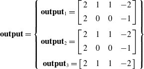 \begin{equation}\textbf{output}=\left\{\begin{array}{c} \textbf{outpu}\textbf{t}_{1}=\left[\begin{array}{c@{\quad}c@{\quad}c@{\quad}c} 2 & 1 & 1 & -2\\[5pt] 2 & 0 & 0 & -1 \end{array}\right]\\[15pt] \textbf{outpu}\textbf{t}_{2}=\left[\begin{array}{c@{\quad}c@{\quad}c@{\quad}c} 2 & 1 & 1 & -2\\[5pt] 2 & 0 & 0 & -1 \end{array}\right]\\[15pt] \textbf{outpu}\textbf{t}_{3}=\left[\begin{array}{c@{\quad}c@{\quad}c@{\quad}c} 2 & 1 & 1 & -2 \end{array}\right] \end{array}\right\} \end{equation}
(3) Step 3: DoF analysis
 \begin{equation}\textbf{DoF}=\left[\begin{array}{c@{\quad}c@{\quad}c@{\quad}c@{\quad}c@{\quad}c@{\quad}c} 1 & 0 & 0 & 0 & 0 & 0 & 0\\[5pt] 0 & 1 & 0 & 0 & 0 & 0 & 0\\[5pt] 0 & 0 & 0 & 0 & 0 & 1 & 0 \end{array}\right]\end{equation}
(4) Step 4: full-cycle mobility determination
There is no “distal” joint existing in the limb. The mechanism has a full-cycle mobility.
-
b. Omni III robot
(1) Step 1: motion matrix could be
 \begin{equation}\textbf{m}=\left[\begin{array}{c} \textbf{m}_{1}=\left[\begin{array}{c@{\quad}c@{\quad}c@{\quad}c@{\quad}c@{\quad}c} 1 & 0 & 0 & 0 & 0 & 0\\[5pt] a_{12} & b_{12} & c_{12} & a_{12} & b_{12} & c_{12}\\[5pt] a_{13} & b_{13} & c_{13} & 0 & 0 & c_{14}\\[5pt] 1 & 0 & 0 & 0 & 0 & c_{14} \end{array}\right]\\[40pt] \begin{array}{c} \textbf{m}_{2}=\left[\begin{array}{c@{\quad}c@{\quad}c@{\quad}c@{\quad}c@{\quad}c} 1 & 0 & 0 & 0 & 0 & 0\\[5pt] a_{22} & b_{22} & c_{22} & a_{22} & b_{22} & c_{22}\\[5pt] a_{23} & b_{23} & c_{23} & 0 & 0 & c_{14}\\[5pt] 1 & 0 & 0 & 0 & 0 & c_{14} \end{array}\right]\\[40pt] \textbf{m}_{3}=\left[\begin{array}{c@{\quad}c@{\quad}c@{\quad}c@{\quad}c@{\quad}c} 1 & 0 & 0 & 0 & 0 & 0\\[5pt] a_{32} & b_{32} & c_{32} & a_{32} & b_{32} & c_{32}\\[5pt] a_{33} & b_{33} & c_{33} & 0 & 0 & c_{14}\\[5pt] 1 & 0 & 0 & 0 & 0 & c_{14} \end{array}\right] \end{array}\\ \\ \textbf{m}_{4}=\left[\begin{array}{c@{\quad}c@{\quad}c@{\quad}c@{\quad}c@{\quad}c} 1 & 0 & 0 & 0 & 0 & 0\\[5pt] a_{42} & b_{42} & c_{42} & a_{42} & b_{42} & c_{42}\\[5pt] a_{43} & b_{43} & c_{43} & 0 & 0 & c_{14}\\[5pt] 1 & 0 & 0 & 0 & 0 & c_{14} \end{array}\right] \end{array}\right]\end{equation}
(2) Step 2: the inputs to the classification optimization would be
 \begin{equation}\textbf{input}=\left[\begin{array}{c} \textbf{inpu}\textbf{t}_{1}=\left[\begin{array}{c@{\quad}c@{\quad}c@{\quad}c@{\quad}c} 1 & 0 & 0 & 1 & -2\\[5pt] 2 & 3 & 4 & 2 & -2\\[5pt] 2 & 3 & 4 & 3 & -2\\[5pt] 2 & 3 & 4 & 0 & -1 \end{array}\right],\textbf{inpu}\textbf{t}_{2}=\left[\begin{array}{c@{\quad}c@{\quad}c@{\quad}c@{\quad}c} 0 & 0 & 1 & 1 & -2\\[5pt] 2 & 3 & 4 & 2 & -2\\[5pt] 2 & 3 & 4 & 3 & -2\\[5pt] 2 & 3 & 4 & 0 & -1 \end{array}\right]\\[30pt] \textbf{inpu}\textbf{t}_{3}=\left[\begin{array}{c@{\quad}c@{\quad}c@{\quad}c@{\quad}c} 0 & 1 & 0 & 1 & -2\\[5pt] 2 & 3 & 4 & 2 & -2\\[5pt] 2 & 3 & 4 & 3 & -2\\[5pt] 2 & 3 & 4 & 0 & -1 \end{array}\right],\textbf{inpu}\textbf{t}_{4}=\left[\begin{array}{c@{\quad}c@{\quad}c@{\quad}c@{\quad}c} 1 & 0 & 0 & 1 & -2\\[5pt] 2 & 3 & 4 & 2 & -2\\[5pt] 2 & 3 & 4 & 3 & -2\\[5pt] 2 & 3 & 4 & 0 & -1 \end{array}\right] \end{array}\right]\end{equation}
The outputs would be
 \begin{equation}\textbf{output}=\left\{\begin{array}{l} \textbf{outpu}\textbf{t}_{1}=\left[\begin{array}{c@{\quad}c@{\quad}c@{\quad}c} 1 & 1 & 3 & -2\\[5pt] 1 & 2 & 3 & -2 \end{array}\right],\textbf{outpu}\textbf{t}_{2}=\left[\begin{array}{c@{\quad}c@{\quad}c@{\quad}c} 1 & 1 & 3 & -2\\[5pt] 1 & 2 & 3 & -2 \end{array}\right]\\[20pt] \textbf{outpu}\textbf{t}_{3}=\left[\begin{array}{c@{\quad}c@{\quad}c@{\quad}c} 1 & 1 & 3 & -2\\[5pt] 1 & 2 & 3 & -2 \end{array}\right],\textbf{outpu}\textbf{t}_{4}=\left[\begin{array}{c@{\quad}c@{\quad}c@{\quad}c} 1 & 1 & 3 & -2\\[5pt] 1 & 2 & 3 & -2 \end{array}\right] \end{array}\right\}\end{equation}
(3) Step 3: DoF analysis
 \begin{equation}\textbf{DoF}=\left[\begin{array}{c@{\quad}c@{\quad}c@{\quad}c@{\quad}c@{\quad}c@{\quad}c} 1 & 0 & 0 & 0 & 0 & 0 & 0\\[5pt] 0 & 1 & 0 & 0 & 0 & 0 & 0 \end{array}\right]\end{equation}
(4) Step 4: full-cycle mobility determination
There is no “distal” joint existing in the limb. The mechanism has a full-cycle mobility.
-
c. 2-PPPHR mechanism
(1) Step 1: motion matrix could be
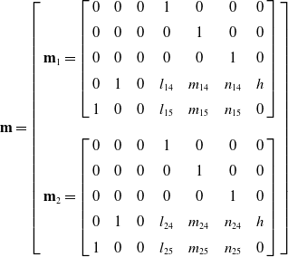 \begin{equation}\textbf{m}=\left[\begin{array}{l} \textbf{m}_{1}=\left[\begin{array}{c@{\quad}c@{\quad}c@{\quad}c@{\quad}c@{\quad}c@{\quad}c} 0 & 0 & 0 & 1 & 0 & 0 & 0\\[5pt] 0 & 0 & 0 & 0 & 1 & 0 & 0\\[5pt] 0 & 0 & 0 & 0 & 0 & 1 & 0\\[5pt] 0 & 1 & 0 & l_{14} & m_{14} & n_{14} & h\\[5pt] 1 & 0 & 0 & l_{15} & m_{15} & n_{15} & 0 \end{array}\right]\\ \\ \textbf{m}_{2}=\left[\begin{array}{c@{\quad}c@{\quad}c@{\quad}c@{\quad}c@{\quad}c@{\quad}c} 0 & 0 & 0 & 1 & 0 & 0 & 0\\[5pt] 0 & 0 & 0 & 0 & 1 & 0 & 0\\[5pt] 0 & 0 & 0 & 0 & 0 & 1 & 0\\[5pt] 0 & 1 & 0 & l_{24} & m_{24} & n_{24} & h\\[5pt] 1 & 0 & 0 & l_{25} & m_{25} & n_{25} & 0 \end{array}\right] \end{array}\right]\end{equation}
(2) Step 2: the inputs to the classification optimization would be
 \begin{equation}\textbf{input}=\left[\begin{array}{l} \textbf{inpu}\textbf{t}_{1}=\left[\begin{array}{c@{\quad}c@{\quad}c@{\quad}c@{\quad}c} 1 & 0 & 0 & 0 & -1\\[5pt] 0 & 1 & 0 & 0 & -1\\[5pt] 0 & 0 & 1 & 0 & -1\\[5pt] 0 & 1 & 0 & 1 & -3\\[5pt] 1 & 0 & 0 & 2 & -2 \end{array}\right]\\ \\ \textbf{inpu}\textbf{t}_{2}=\left[\begin{array}{c@{\quad}c@{\quad}c@{\quad}c@{\quad}c} 1 & 0 & 0 & 0 & -1\\[5pt] 0 & 1 & 0 & 0 & -1\\[5pt] 0 & 0 & 1 & 0 & -1\\[5pt] 0 & 1 & 0 & 1 & -3\\[5pt] 1 & 0 & 0 & 2 & -2 \end{array}\right] \end{array}\right]\end{equation}
The outputs would be
 \begin{equation}\textbf{output}=\left\{\begin{array}{l} \textbf{outpu}\textbf{t}_{1}=\left[\begin{array}{c@{\quad}c@{\quad}c@{\quad}c} 2 & 0 & 0 & -1 \end{array}\right]\\[10pt] \textbf{outpu}\textbf{t}_{2}=\left[\begin{array}{c@{\quad}c@{\quad}c@{\quad}c} 2 & 0 & 0 & -1 \end{array}\right] \end{array}\right\}\end{equation}
(3) Step 3: DoF analysis
 \begin{equation}\textbf{DoF}=\left[\begin{array}{c@{\quad}c@{\quad}c@{\quad}c@{\quad}c@{\quad}c@{\quad}c} 1 & 0 & 0 & 0 & 0 & 0 & 0\\[5pt] 0 & 1 & 0 & 0 & 0 & 0 & 0\\[5pt] 0 & 0 & 0 & 1 & 0 & 0 & 0\\[5pt] 0 & 0 & 0 & 0 & 1 & 0 & 0\\[5pt] 0 & 0 & 0 & 0 & 0 & 1 & 0 \end{array}\right]\end{equation}
(4) Step 4: full-cycle mobility determination
There is no “distal” joint existing in the limb. The mechanism has a full-cycle mobility.


