1. Introduction
Fast radio bursts (FRBs) are a type of highly energetic astrophysical transient that last only a few milliseconds (e.g. Lorimer et al. Reference Lorimer, Bailes, McLaughlin, Narkevic and Crawford2007). Many FRBs have dispersion measures (DMs) that exceed the expected maximum of the Galactic electron density, indicating their extragalactic origins. DM represents the column density of free electrons traversed along the propagation path of an FRB. Despite their discovery over a decade ago (Lorimer et al. Reference Lorimer, Bailes, McLaughlin, Narkevic and Crawford2007), the origin of FRBs remains a mystery. Recently, the detection of repeating FRBs (e.g., Spitler et al. Reference Spitler2014; Niu et al. Reference Niu2022) has opened up new avenues of research into the origin of these phenomena.
With the emergence of a large number of FRBs samples in recent years, repeated FRBs (referred to as ‘repeating bursts’ for simplicity) have also been noticed by astronomers, especially FRB 20121102A, which has been observed to have a very high burst rate (e.g., Li et al. Reference Li2021; Jahns et al. Reference Jahns2022). FRB 20121102A is the first-discovered repeating FRB source (Scholz et al. Reference Scholz2016). This source was first recorded in 2012 and was detected again in the same spatial location in 2015 with the same dispersion measure (Scholz et al. Reference Scholz2016). In subsequent observations, FRB 20121102A exhibited an extremely high repetition rate compared to other FRBs (e.g., Li et al. Reference Li2021; Jahns et al. Reference Jahns2022) and became the first repeating burst to be localized (Chatterjee et al. Reference Chatterjee2017).
Given the large sample size of recent FRB detections (e.g., Li et al. Reference Li2021), machine-learning approaches have been becoming important. Applying deep learning to single-pulse classification was proposed in a pioneering paper by Connor & van Leeuwen (Reference Connor and van Leeuwen2018). They trained a deep neural network using single pulses and false-positive triggers from real telescopes to develop a framework for ranking events. The ranking was ordered by their probability of being astrophysical transients with high accuracy, recall, and quick computational time, indicating the power of deep learning.
Since then, unsupervised machine learning has been applied to the Canadian Hydrogen Intensity Mapping Experiment (CHIME) data (e.g., Chen et al. Reference Chen, Hashimoto, Goto, Kim, Santos, On, Lu and Hsiao2022; Zhu-Ge, Luo, & Zhang Reference Zhu-Ge, Luo and Zhang2023). Chen et al. (Reference Chen, Hashimoto, Goto, Kim, Santos, On, Lu and Hsiao2022) and Zhu-Ge, Luo, & Zhang (Reference Zhu-Ge, Luo and Zhang2023) found distinct physical properties (i.e. the ratio of the highest frequency to the peak frequency by Chen et al. Reference Chen, Hashimoto, Goto, Raquel, Uno, Kim, Hsiao and Ho2023, brightness temperature and rest-frame frequency bandwidth by Zhu-Ge, Luo, & Zhang Reference Zhu-Ge, Luo and Zhang2023) between repeaters and one-off events, which allows the machine to predict the repetitiveness of FRBs. Based on the unsupervised machine learning approaches, both studies identified some potentially repeating FRBs currently reported as one-off FRBs. A few active repeaters, including FRB 20201124A (Chen et al. Reference Chen, Hashimoto, Goto, Raquel, Uno, Kim, Hsiao and Ho2023) and FRB 20121102A (Raquel et al. Reference Raquel, Hashimoto, Goto, Chen, Uno, Hsiao, Kim and Ho2023), were also classified by unsupervised machine algorithm. Some distinct clusters were commonly identified for these active repeating FRB sources, suggesting multiple radiation mechanisms of active repeaters or distinct physical environments of emission regions. These approaches to the FRB classification used catalogs, including measured physical properties of individual FRBs. In addition to such catalog-based classifications, the UMAP algorithm was used for the image data (i.e. waterfall) of the CHIME FRBs (Yang et al. Reference Yang, Zhang, Wang and Wu2023). They found that the UMAP algorithm using image data produced more accurate results in predicting the repetitiveness.
In this paper, we revisit the repeating FRB 20121102A using Arecibo samples (Jahns et al. Reference Jahns2022) with a machine-learning classification, being free of human bias, an approach to understanding its properties and origin. The uniform manifold approximation and Projection (UMAP) (McInnes, Healy, & Melville Reference McInnes, Healy and Melville2018; McInnes et al. Reference McInnes, Healy, Saul and Großberger2018) is an algorithm that utilizes manifold learning techniques and incorporates concepts from topological data analysis to achieve dimension reduction. It offers a versatile framework for approaching manifold learning and dimension reduction, providing both a broad scope and specific practical implementations. This paper aims to explain the practical workings of the UMAP algorithm. UMAP is useful because it allows the two-dimensional projection of higher-dimensional data points, which can be handled easily. Previous studies demonstrate the effectiveness of UMAP and the practical usage of a follow-up science case. Kim et al. (Reference Kim, Hashimoto, Chen and Goto2022), Chen et al. (Reference Chen, Hashimoto, Goto, Kim, Santos, On, Lu and Hsiao2022)
After the classification, we make a comparison between this work and the previous machine learning classification result using Five hundred meter Aperture Spherical Telescope (FAST) data (Raquel et al. Reference Raquel, Hashimoto, Goto, Chen, Uno, Hsiao, Kim and Ho2023) to mitigate a possible observational bias. We note that the Arecibo samples include relatively brighter FRB populations (
![]() $\gtrsim$
0.095 Jy ms; Jahns et al. Reference Jahns2022) than those in the FAST samples (
$\gtrsim$
0.095 Jy ms; Jahns et al. Reference Jahns2022) than those in the FAST samples (
![]() $\gtrsim$
0.02 Jy ms; Li et al. Reference Li2021), making this work independent of Raquel et al. (Reference Raquel, Hashimoto, Goto, Chen, Uno, Hsiao, Kim and Ho2023). We investigate whether there are groups with common features between the FAST and Arecibo data so that we can corroborate the previous classification result with conjectures about the origin.
$\gtrsim$
0.02 Jy ms; Li et al. Reference Li2021), making this work independent of Raquel et al. (Reference Raquel, Hashimoto, Goto, Chen, Uno, Hsiao, Kim and Ho2023). We investigate whether there are groups with common features between the FAST and Arecibo data so that we can corroborate the previous classification result with conjectures about the origin.
2. Data pre-processing
We use the FRB catalogue detected in the Arecibo archival data (Jahns et al. Reference Jahns2022). The catalogue includes a total of 849 FRBs from the identical source of FRB 20121102A. Each FRB can contain multiple sub-bursts. There are 988 sub-bursts in total in the catalogue (classified by visual inspection). In this work, we treat sub-bursts independently, following Raquel et al. (Reference Raquel, Hashimoto, Goto, Chen, Uno, Hsiao, Kim and Ho2023). To ensure adherence to physical principles, all data points with negative amplitudes were removed, resulting in the final samples of 977 FRB sub-bursts. The catalogue contains the following parameters:
-
• Time of arrival (ms)
-
• Amplitude (A)
-
• Bandwidth (sig_nu) (MHz)
-
• Central frequency (nu_0) (MHz)
-
• Dispersion Measure (
 $\mathrm{pc}\,\cdot\,\mathrm{cm}^{-3}$
)
 -
• Linear temporal drift (d) (
 $\mathrm{ms}\,\cdot\,\mathrm{MHz}^{-1}$
)
 -
• Fluence (
 $\mathrm{Jy}\,\cdot\,\mathrm{ms}$
)
 -
• Time duration (sig_t) (ms)
-
• Scaled energy (erg).
We exclude the time of arrival in this work because it can only convey the sequence of arrival of various FRBs, and its correlation with physical properties is limited. In other words, the time of arrival alone would not be closely related to the distinct physical characteristics of each FRB.
Equation (2) in (Jahns et al. Reference Jahns2022) fits two-dimensional, elliptical Gaussians to each sub-burst in the burst spectra. The exact form depending on time t and radio frequency
![]() $\nu$
is
$\nu$
is
The variable A represents the amplitude of the fitting function.
Following Raquel et al. (Reference Raquel, Hashimoto, Goto, Chen, Uno, Hsiao, Kim and Ho2023), we also exclude DM from the classification process since the repeating FRBs from the FRB 20121102A source have almost the same DMs. In other words, each burst in FRB 20121102A exhibits an almost identical DM. Therefore, including it in the classification process would not provide significant and meaningful information. The fluence is a readily quantifiable property of a transient that remains less affected by the time resolution of the observation (e.g., Macquart & Ekers Reference Macquart and Ekers2018; Hashimoto et al. Reference Hashimoto2022). Therefore, we use fluences provided by Jahns et al. (Reference Jahns2022) rather than using flux densities.
In summary, we utilise seven parameters (Jahns et al. Reference Jahns2022), including: Amplitude (corresponding to the fitting relation, as seen in Equation 1), Linear temporal drift (temporal change of the peak frequency), Time duration (temporal burst width), Central frequency (spectral peak), Bandwidth (width in the frequency domain), Scaled energy (the isotropic equivalent energy that is scaled from the fluence and the 2D Gaussian fits), Fluence (the flux of FRBs integrated over the time duration).
These parameters collectively contribute to the analysis presented in this study.
3. Data processing/methodology
3.1 Unsupervised machine learning
UMAP is an innovative manifold learning technique used for dimension reduction. It is built on a theoretical foundation rooted in Riemannian geometry and algebraic topology (McInnes, Healy, & Melville Reference McInnes, Healy and Melville2018; McInnes et al. Reference McInnes, Healy, Saul and Großberger2018). After pre-processing, our data consists of 977 rows and 7 columns. To facilitate data visualization and conduct unsupervised learning, we employ the UMAP algorithm. Here are our processing steps:
-
1. Embedding the data with the following hyperparameter of n_neighbors. Embedding refers to the process of mapping high-dimensional data points to a lower-dimensional space while preserving certain structural relationships and patterns present in the data. The goal of embedding is to represent complex and high-dimensional data in a more visually interpretable form, typically in two or three dimensions, without losing important information (e.g., McInnes, Healy, & Melville Reference McInnes, Healy and Melville2018; McInnes et al. Reference McInnes, Healy, Saul and Großberger2018; Chen et al. Reference Chen, Hashimoto, Goto, Kim, Santos, On, Lu and Hsiao2022). n_neighbors is one of UMAP’s basic hyperparameters, which significantly affect the resulting embedding of the data (e.g., Raquel et al. Reference Raquel, Hashimoto, Goto, Chen, Uno, Hsiao, Kim and Ho2023).
-
2. Clustering analysis with Hierarchical Density-Based Spatial Clustering of Applications with Noise (HDBSCAN) (Campello, Moulavi, & Sander Reference Campello, Moulavi and Sander2013) to identify a group(s) in the embedded data.
-
3. Testing the processes 1 and 2 with different values of n_neighbors. We investigate n_neighbors
 $=$
5,6,7,8, and 9 in this work. The embedding and clustering results of n_neighbors
 $=$
5,6,7, and 9 are presented in APPENDIX A (Fig. A1), whereas we adopt n_neighbors
 $=$
8 as the fiducial result (see Section 3.2 for details).
 -
4. Determining the optimised n_neighbors, which maximizes the ‘rand score’. The concept of the rand score is introduced in the next section, which delves into the evaluation of similarities among different n_neighbors outcomes. This evaluation aims to identify which results exhibit the highest degree of agreement with others.
-
5. Parameter colouring and histograms to investigate the characteristics of each cluster based on the optimised n_neighbors.
3.2 Rand score for clustering performance
Because this is an unsupervised ML, we need Rand Score to make the comparison. A clustering performance metric, namely the Rand Index (Hubert & Arabie Reference Hubert and Arabie1985), and its adjusted form provide us with a Rand score and Adjusted Rand score for each pair of compared different n_neighbors clustering results. A high score indicates that the two clustering results are in excellent agreement (e.g., Hubert & Arabie Reference Hubert and Arabie1985; Raquel et al. Reference Raquel, Hashimoto, Goto, Chen, Uno, Hsiao, Kim and Ho2023). A higher Rand score indicates a greater similarity with the classification results of other n_neighbors values, i.e. a high Rand Score (high agreement) agrees with another result. To find the most suitable n_neighbors, we need to find the rand score of each pair of n_neighbors. In Fig. 1, the adjusted rand score is compared with the rand score with each point annotated with the pair of n_neighbors. In this work, we choose n_neighbors = 8, which has the highest rand score compared with the other values of n_neighbors, and is included in the 2nd highest rand score. This way, even by considering only one of these results for discussion, we could extract the common groups for the different values of n_neighbors. The details of n_neighbors and rand score arguments are presented in Chen et al. (Reference Chen, Hashimoto, Goto, Kim, Santos, On, Lu and Hsiao2022) and Raquel et al. (Reference Raquel, Hashimoto, Goto, Chen, Uno, Hsiao, Kim and Ho2023), respectively.
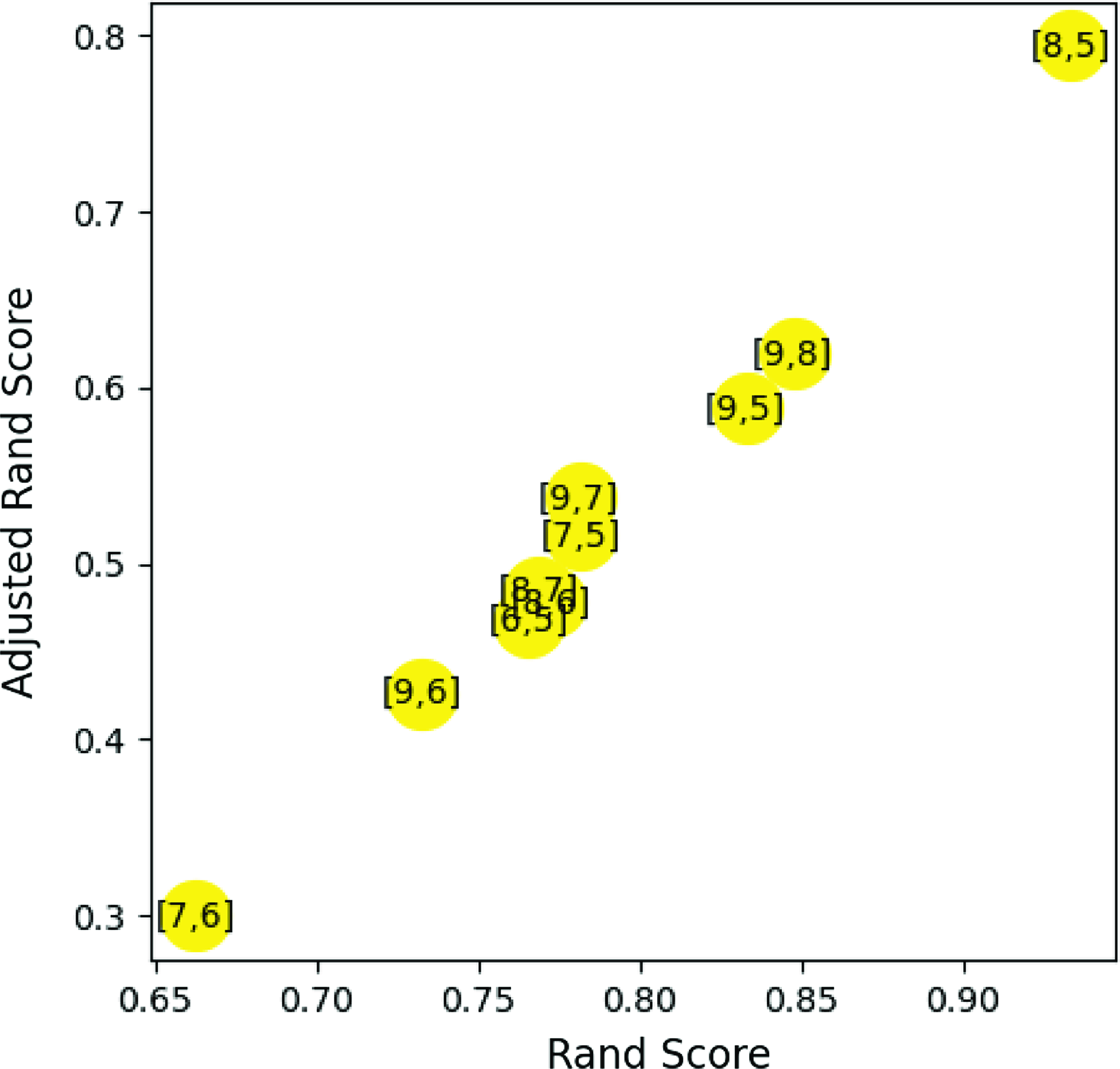
Figure 1. Adjusted Rand Score as a function of Rand Score. Higher values of Adjusted Rand Score and Rand Score indicate a greater similarity of the classification results between the pair of n_neighbors values. The pair of n_neighbors = 8 and 5 shows the highest Adjusted Rand Score and Rand Score, indicating that n_neighbors = 8 clustering result is most similar to that of n_neighbors
![]() $=5$
. n_neighbors = 8 is commonly included in the two highest cases.
$=5$
. n_neighbors = 8 is commonly included in the two highest cases.
3.3 Hyperparameters
There are two sets of hyperparameters in this study. The first set is of the UMAP and the second set is the HDBSCAN. UMAP hyperparameters that are considered in this study are min_dist, metric, n_components, and n_neighbours.
min_dist controls the clumping of the embedded data points which means that the smaller the value we assign to this hyperparameter the clumpier the resulting embedding would be. Thus, in this study, we set min_dist = 0.01.
metric is essentially the way distance is defined on the resulting embedding. Since using other metrics is not intuitive or straightforward, we set metric
![]() $=$
Euclidean.
$=$
Euclidean.
n_components dictates the spatial dimension of the resulting embedding. Thus, for simplicity and ease of visualization, we set n_components
![]() $= 2$
.
$= 2$
.
n_neighbours is the most important hyperparameter in this stage. This hyperparameter estimates the manifold structure by controlling the size of the local neighborhood. This suggests that a lower value would emphasize the regional structure compared to a higher value which then emphasizes the global structure. Thus in this study, we set n_neighbors
![]() $= 8$
(see also Section 3.2 for details).
$= 8$
(see also Section 3.2 for details).
HDBSCAN compared to UMAP has a larger number of hyperparameters, however only four major parameters significantly affect the resulting clustering. These hyperparameters are min_cluster_size, min_samples,
cluster_selection_epsilon, and alpha.
min_cluster_size is the size of the grouping that can be considered a cluster. This in return affects the number of clusters that can be identified by HDBSCAN. In this study the value of min_cluster_size
![]() $= 80$
because after numerous trials with different values ranging between 30 and 100, we found that setting min_cluster_size
$= 80$
because after numerous trials with different values ranging between 30 and 100, we found that setting min_cluster_size
![]() $= 80$
resulted in more significant differences between the parameters of the clusters. Also, it can be classified clearly between clusters and noises.
$= 80$
resulted in more significant differences between the parameters of the clusters. Also, it can be classified clearly between clusters and noises.
min_samples is also an important hyperparameter and should be considered depending on the resulting embedding. When a large value is used for this hyperparameter, a large number of points will then be considered Noise. Thus, the researchers set a conservative value of min_samples
![]() $= 15$
since the default setting of min_samples was found to be the most appropriate value after thorough examinations. This process involved checking whether some data points were mistakenly considered as noise, despite their values and errors conforming to reasonable physical interpretations.
$= 15$
since the default setting of min_samples was found to be the most appropriate value after thorough examinations. This process involved checking whether some data points were mistakenly considered as noise, despite their values and errors conforming to reasonable physical interpretations.
cluster_selection_epsilon controls the merging of microclusters located in high-concentration regions when tuned correctly. However, adjusting this hyperparameter to merge microclusters will not provide further insight into the clustering aside from the fact that they are considered a group or a cluster. Therefore, we set cluster_selection_epsilon
![]() $= 0$
which is its default value.
$= 0$
which is its default value.
alpha is a hyperparameter that is rarely adjusted, if not avoided, and only acts as a last resort when tuning min_samples or cluster_selection_epsilon, which does not provide any useful changes to the clustering. This hyperparameter is used to determine how conservative the clustering will become but since its adjustment is not necessary, we set it to its default value of alpha
![]() $=1.0$
.
$=1.0$
.
4. Results
4.1 Embedding and clustering results
The embedding result with n_neighbors = 8 is shown as Fig. 2. Fig. 2 shows distinct data distributions, indicating the existence of multiple clusters in the data. The clustering algorithm described in Section 3.1 is applied to Fig. 2 to identify clusters. The embedded data are classified into five clusters as shown in Fig. 2. The clusters are clearly separated from each other, demonstrating the distinct distribution of each cluster. Distinct clusters are assigned unique colours to represent groups of data points (Fig. 2). The distinct characteristics of these clusters are elaborated in Section 4.2.
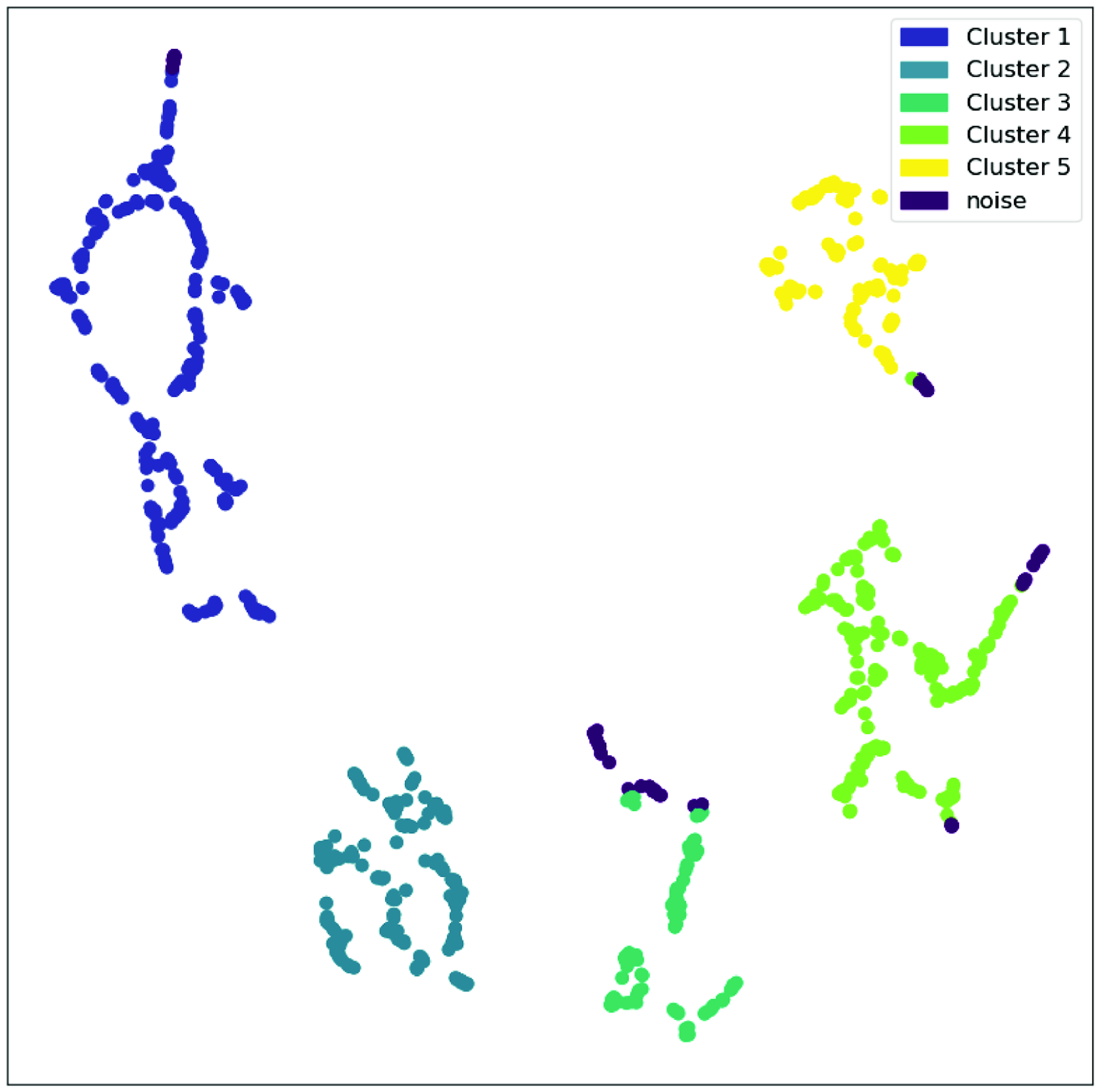
Figure 2. Two-dimensional UMAP embedding for n_neighbors=8. The 977 FRB data are classified into five clusters with n_neighbors=8. After ‘projection’, HDBSCAN (Campello, Moulavi, & Sander Reference Campello, Moulavi and Sander2013) is utilised to identify individual groups.
4.2 Identifying characteristic properties of each cluster
Because there are seven parameters in our analysis, we show seven plots of embedded data with colouring for each of the seven parameters in Figs. 3 and 4. These colouring plots allow us to infer the distinct characteristics of each cluster.
To validate the characteristics of clusters, we construct histograms, followed by analysis and summarization in the form of tables, Tables 1 and 2. In the histograms provided in Fig. 5, we conducted an examination of the Amplitude Fig. 5a, Bandwidth Fig. 5b, Central Frequency Fig. 5c, Linear Temporal Drift Fig. 5d, Fluence Fig. 6a, Scaled Energy Fig. 6b, and Time Duration Fig. 6c histograms. Notably, the bandwidth distributions exhibited unique patterns in all clusters, supporting that the resulting clusters are significantly different.
Table 1. Average value of each parameter in each cluster with n_neighbors=8. The errors include two significant figures. For the purpose of comparing with the Critical Temperature (Xiao & Dai Reference Xiao and Dai2022), we computed the Brightness Temperature (BT) using the average values of each parameter, as presented in the last row.

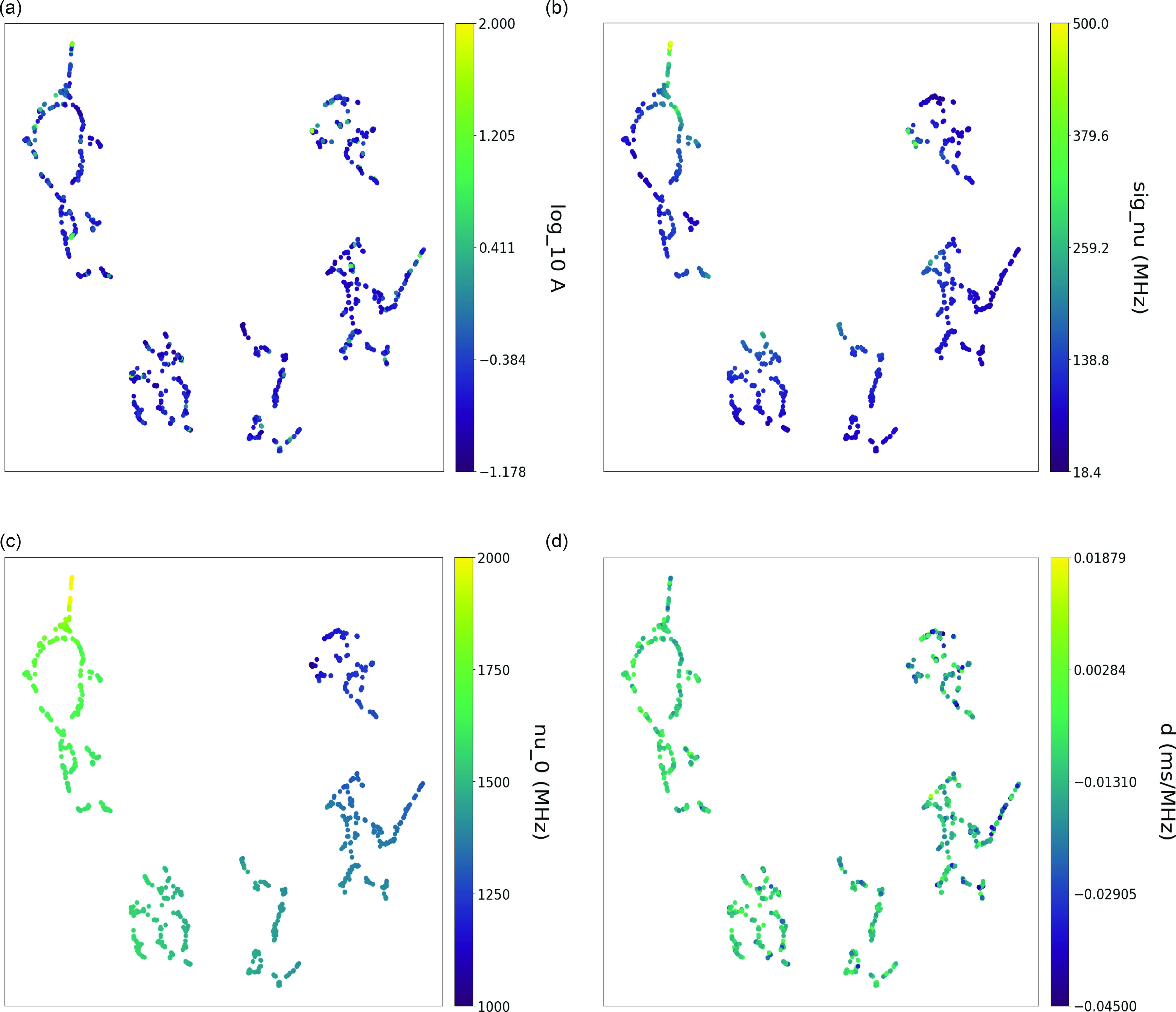
Figure 3. Parameter colouring of the clustering result for n_neighbors = 8. From (a) to (d), the amplitude, bandwidth, central frequency, and linear temporal drift are shown, respectively. For amplitude (a), the colour is shown in the logarithmic scale for visualization purposes.
Table 2. Cluster properties that remain constant with n_neighbors=8. The qualitative description of the clusters is based on the range of values for each parameter of a given cluster.
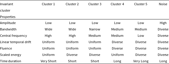
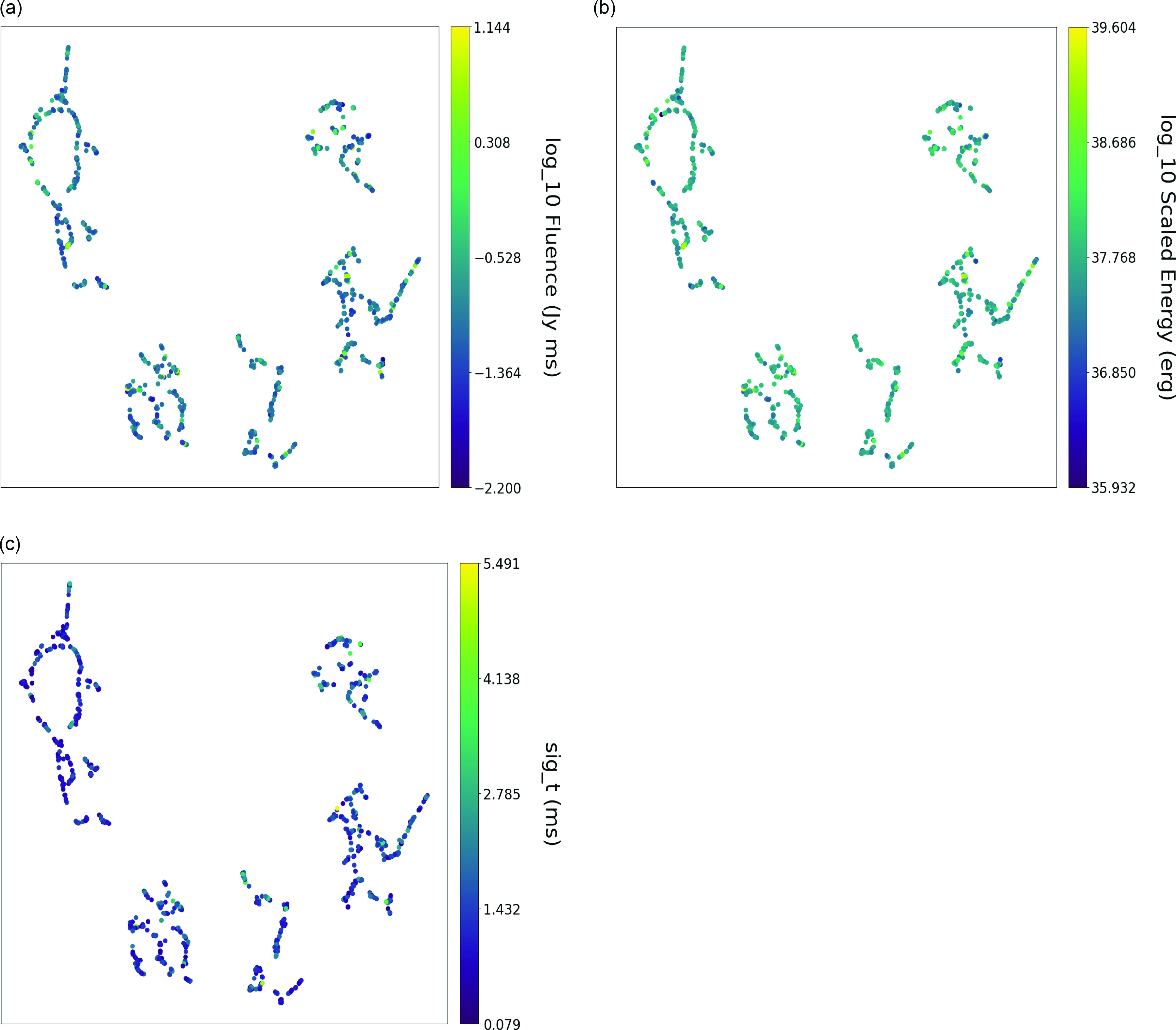
Figure 4. Parameter colouring of the clustering result for n_neighbors = 8. From (a) to (c), the fluence, scaled energy, and time duration are shown, respectively.
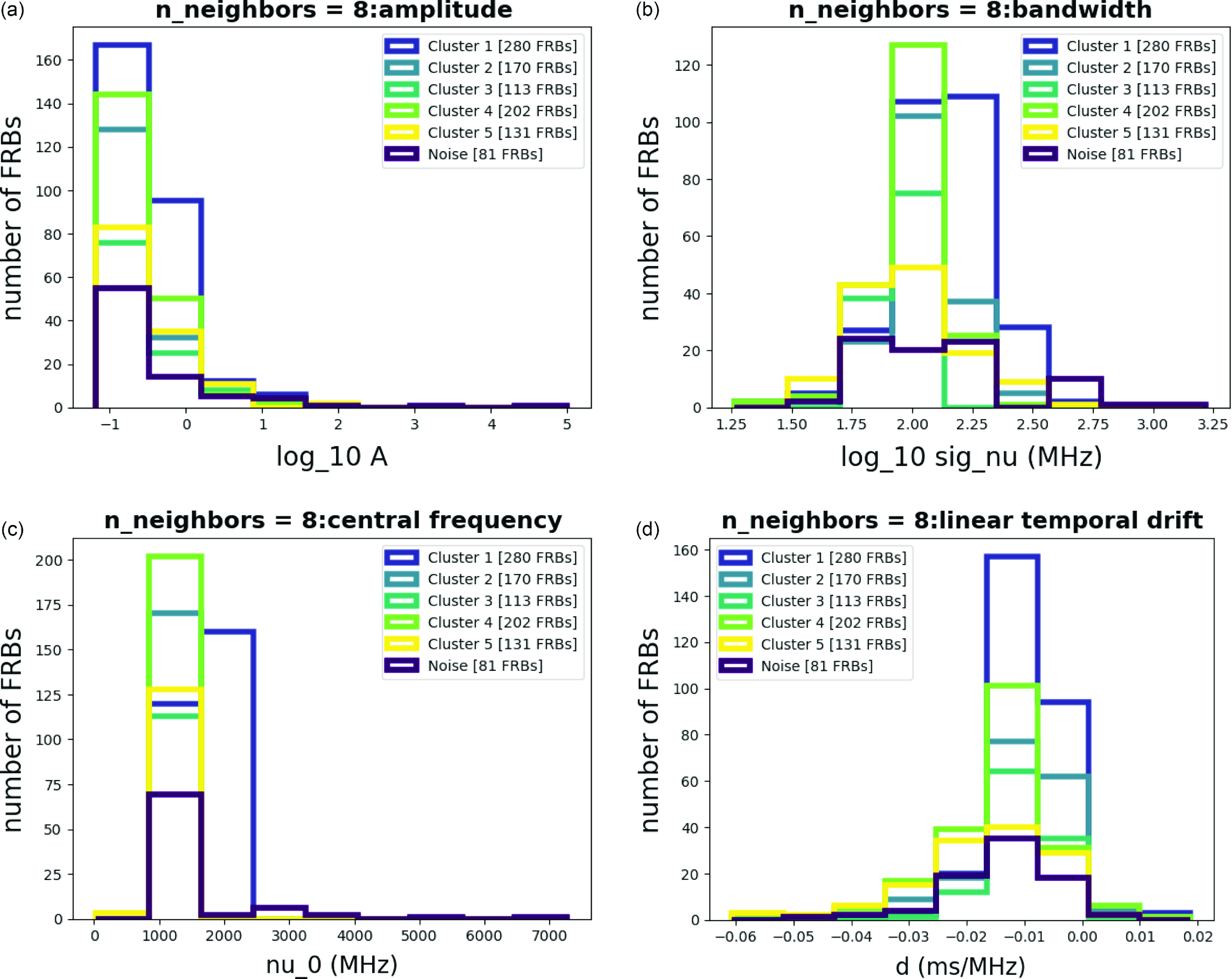
Figure 5. Histograms for each parameter with n_neighbors = 8.
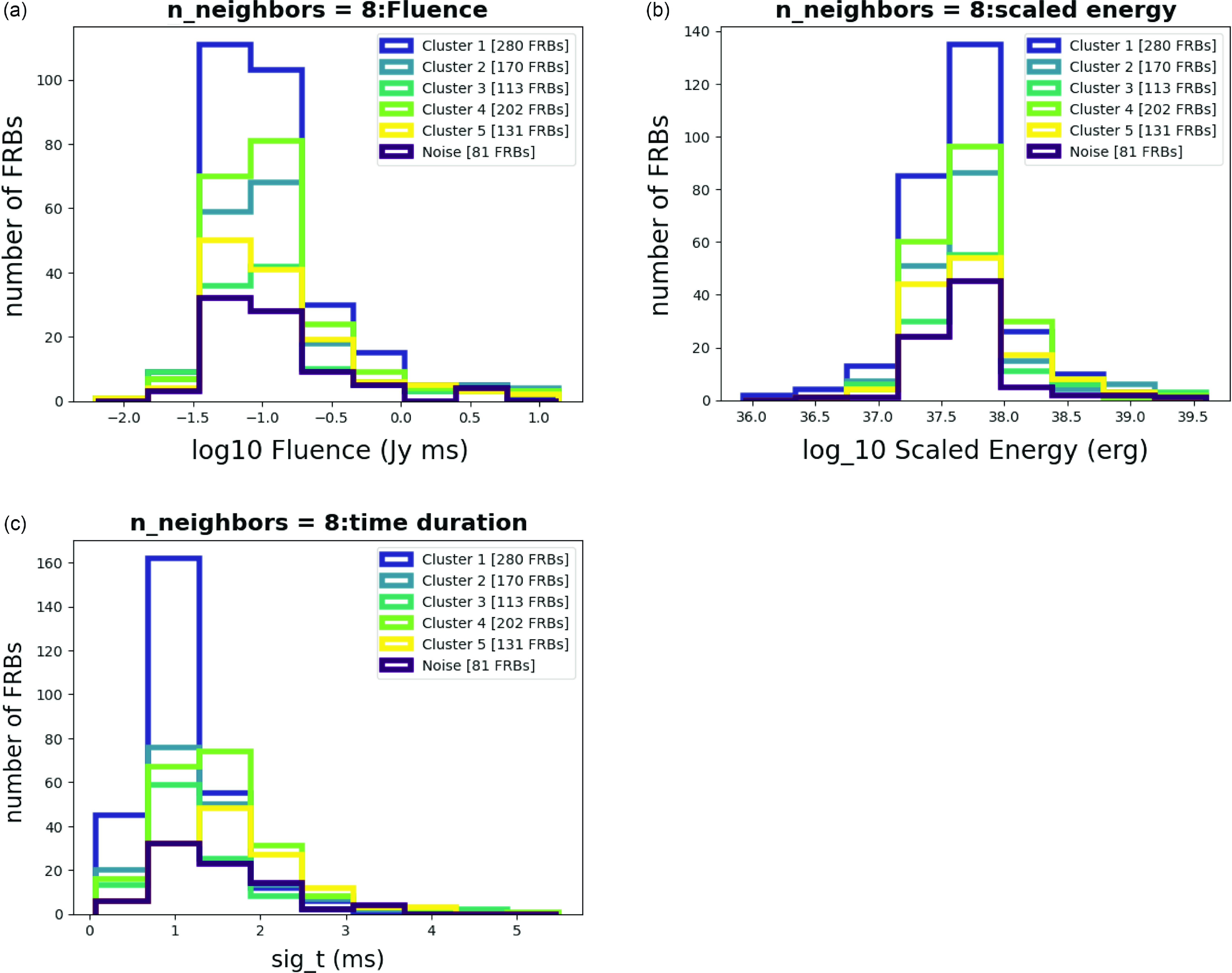
Figure 6. Parameter colouring of the clustering result for n_neighbors = 8.
We combine the results of histograms and colouring figures for discussion. Some parameters clearly show distinct differences among each cluster, especially central frequency and bandwidth. While others may appear less distinguishable, we carefully examine their distribution patterns, noting some are wider in the frequency domain while others are narrower. This allows us to identify the unique characteristics of each cluster.
The result of the analysis is summarized in Tables 1 and 2. As shown in Table 2, each cluster encompasses a distinct set of attributes, as illustrated in the Appendix (Amplitude Fig. A2, Bandwidth Fig. A3, Central Frequency Fig. A4, Fluence Fig. A5, Scaled Energy Fig. A6, and Time Duration Fig. A7). Even with varying n_neighbor values, each cluster exhibits similar distributions, as seen in Table 2. We might refer to these attributes as ‘invariant’ cluster properties. Although these attributes do not immediately pin point us to specific physical mechanisms, the classyfying is an important step advance, because now we can try to theoretically understand each cluster one by one, instead of understanding them all at once while mixed.
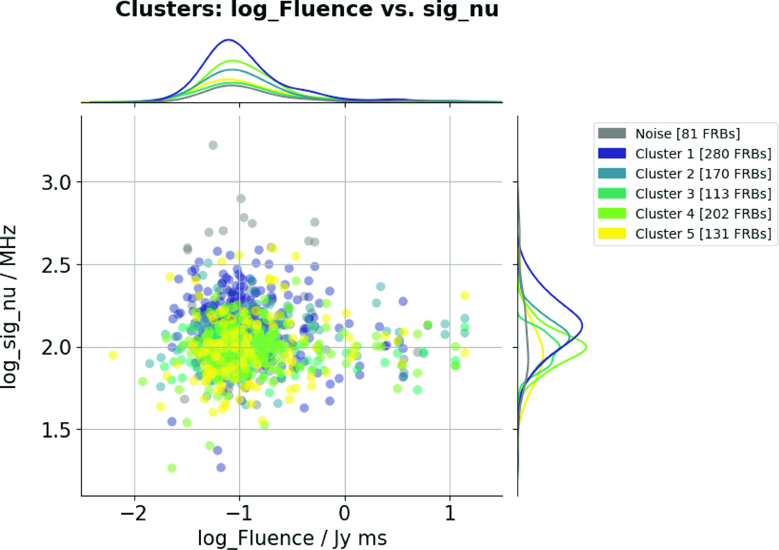
Figure 7. Mapping plot of Bandwidth and Fluence with n_neighbors=8. Different colors correspond to different clusters. The histograms on the vertical and horizontal axes represent the data distributions of Bandwidth and Fluence, respectively.
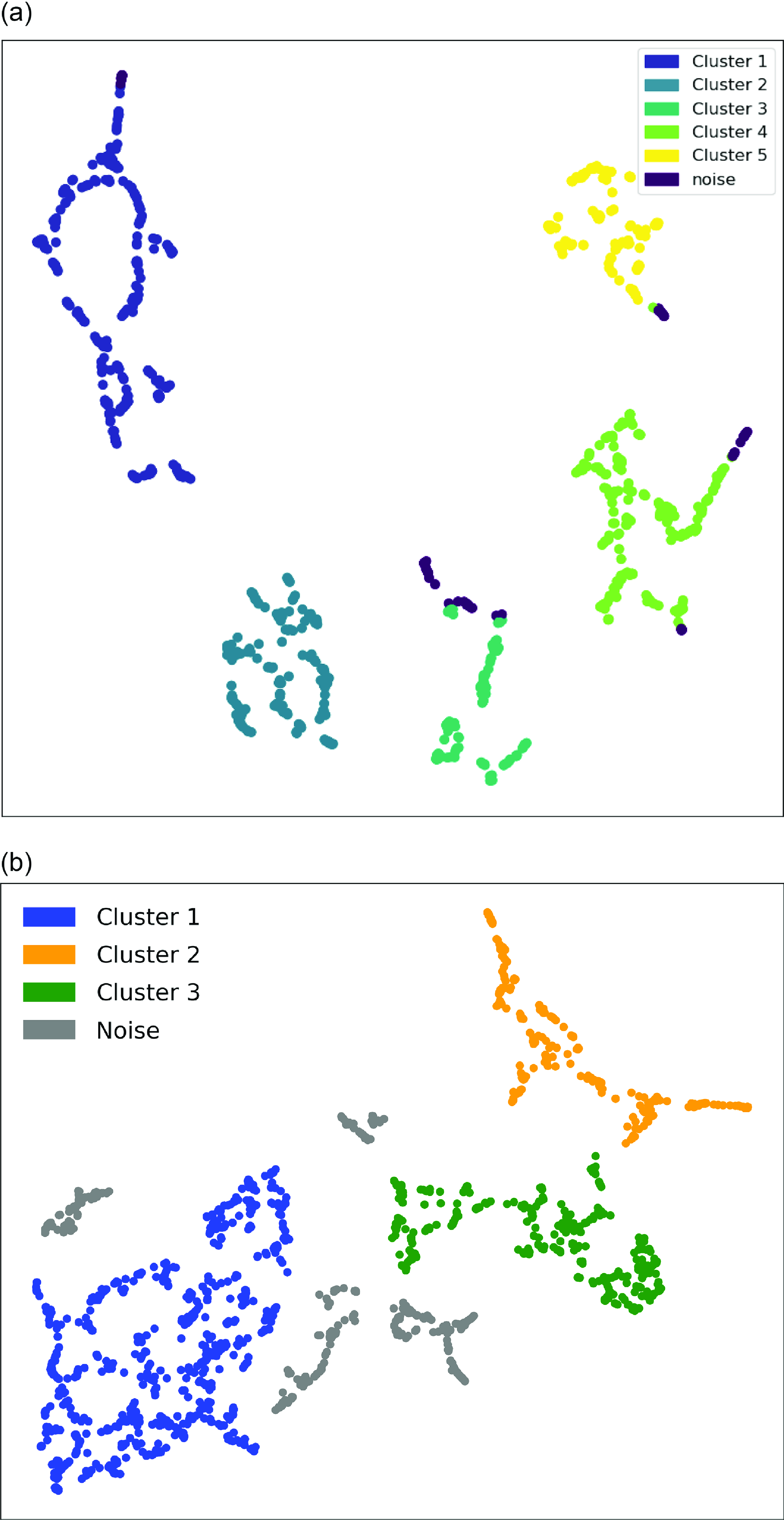
Figure 8. The comparison of the clustering of our result (a) and Raquel et al. (Reference Raquel, Hashimoto, Goto, Chen, Uno, Hsiao, Kim and Ho2023) (b).
5. Discussion
5.1 Relationships between different variables
After performing dimensionality reduction on the clusters, we aimed to map these clusters onto joint distribution plots of the variables. To identify significant differences, we selected physical parameters that showed notable variations between clusters. We will discuss these differences following the analysis of histograms (Figs. 5, 6) and tables (Tables 1 and 2). We observe that Fluence and Bandwidth exhibit the most significant differences among clusters, as shown in the histograms in Figs. 5 and 6, and the data in Tables 1 and 2. To further analyze these parameters, we combined and mapped them into a distribution plot (Fig. 7). In Fig. 7, the distribution of Fluence in Cluster 1 appears more concentrated compared to the other clusters, and so does the distribution of Bandwidth, indicating that most of the FRBs in Cluster 1 are similar.
Additionally, there is a subtle secondary peak beside the main peak in the distribution curve of Cluster 1. This raises an interesting question: could there be a physical mechanism that generates two extremums of Fluence, unlike other mechanisms that result in a single peak, as observed in the other Clusters?
As for the Bandwidth of each cluster, there are noticeable differences between their peaks, especially between Cluster 1 and Cluster 4. There is also something interesting that the Bandwidth distribution of Cluster 3 has two significant peaks. It would be valuable to explore what causes these significant differences in future work.
5.2 Comparison with the classification by the previous work
We compare our classification with another classification result of FRB 20121102A using the FAST data (Raquel et al. Reference Raquel, Hashimoto, Goto, Chen, Uno, Hsiao, Kim and Ho2023). Our result, presented in Fig. 8a, shows five clusters, while Fig. 8b from Raquel et al. (Reference Raquel, Hashimoto, Goto, Chen, Uno, Hsiao, Kim and Ho2023) shows three clusters. Noises are also plotted in the figures.
Figs. 9 and 10 compare the colouring results between Raquel et al. (Reference Raquel, Hashimoto, Goto, Chen, Uno, Hsiao, Kim and Ho2023) and this work for parameters commonly used in both studies. Figs. 10a and b are the energy (Raquel et al. Reference Raquel, Hashimoto, Goto, Chen, Uno, Hsiao, Kim and Ho2023) and scaled energy (this work) colouring of the clustering results, respectively. The scaled energy represents the isotropic equivalent energy, derived by scaling the fluence and the 2D Gaussian fits using Equation 2 in Jahns et al. (Reference Jahns2022). In Fig. 9, both Cluster 2 in Raquel et al. (Reference Raquel, Hashimoto, Goto, Chen, Uno, Hsiao, Kim and Ho2023) and Cluster 1 in this work show higher Bandwidths than the other clusters. These clusters also include FRBs with high Fluence (Fig. 9c and d) and high Energy/Scaled Energy (Fig. 10a and b). Therefore, we speculate that Cluster 2 in Raquel et al. (Reference Raquel, Hashimoto, Goto, Chen, Uno, Hsiao, Kim and Ho2023) is a similar population to Cluster 1 in this work.
Cluster 3 in Raquel et al. (Reference Raquel, Hashimoto, Goto, Chen, Uno, Hsiao, Kim and Ho2023) includes FRBs with two distinct properties with low and high values of Bandwidth (Fig. 9a), Fluence (Fig. 9c), Energy (Fig. 10a), and Time Width (Fig. 10c). These properties of Cluster 3 in Raquel et al. (Reference Raquel, Hashimoto, Goto, Chen, Uno, Hsiao, Kim and Ho2023) would correspond to a combination of Cluster 4 and 5 in this work. The remaining Cluster 1 in Raquel et al. (Reference Raquel, Hashimoto, Goto, Chen, Uno, Hsiao, Kim and Ho2023) shows similar physical properties to a combination of Cluster 2 and 3 in this work in terms of Bandwidth/sig_nu, Fluence, Energy/Scaled Energy, and Time Width/sig_t (Figs. 9 and 10). Therefore, we circle borders with similar colours and shapes to individual clusters that might correspond to each other (e.g. their Cluster 2 might correspond to our Cluster 1. Therefore, we encircle Cluster 1 with a yellow dashed line, just as they encircled their Cluster 2 with a yellow dashed line).
We found five clusters with noise, each of which possesses distinct physical properties. This suggests that FRBs might involve multiple different physical mechanisms, leading to individual sets of radio emissions with unique characteristics. The geometry of the emission region and the propagation effect of FRB signals could also make such distinct clusters. However, the previous analysis by Raquel et al. (Reference Raquel, Hashimoto, Goto, Chen, Uno, Hsiao, Kim and Ho2023) identified three different clusters, whereas our result includes five. We speculate the following reasons for the different numbers of clusters between Raquel et al. (Reference Raquel, Hashimoto, Goto, Chen, Uno, Hsiao, Kim and Ho2023) and this work:
-
1. Their analysis yielded three clusters (Raquel et al. Reference Raquel, Hashimoto, Goto, Chen, Uno, Hsiao, Kim and Ho2023), but this does not necessarily mean there are only three distinct groups. FAST telescope is larger and more sensitive than Arecibo. Therefore, their data are dominated by fainter bursts than ours. This may have led them to miss clusters dominated by brighter bursts. For example, our cluster 1 and 4 include brighter bursts.
-
2. Differences in the parameters used in our study compared to theirs (Raquel et al. Reference Raquel, Hashimoto, Goto, Chen, Uno, Hsiao, Kim and Ho2023) may lead to variations in the machine learning outcomes. One contri- buting factor may be the omission of noise during their analysis.
5.3 Critical Temperature
The Critical Temperature serves as a criterion for distinguishing between Classical and Atypical bursts proposed by Xiao & Dai (Reference Xiao and Dai2022) using FAST data of FRB 20121102A. Following Xiao & Dai (Reference Xiao and Dai2022), we investigate the Critical Temperature of the Arecibo data (Jahns et al. Reference Jahns2022) in this work. We compute the average Brightness Temperature (BT) values for each cluster, which are presented as the bottom row in Table 1. BTs of Cluster 2, 3, and 5 exceed the Critical BT of
![]() $10^{33}$
K proposed by Xiao & Dai (Reference Xiao and Dai2022). The errors of BTs in Cluster 1, 4, and Noise are too large to determine whether their BTs exceed the Critical BT. The average BT in Cluster 3 is significantly higher than
$10^{33}$
K proposed by Xiao & Dai (Reference Xiao and Dai2022). The errors of BTs in Cluster 1, 4, and Noise are too large to determine whether their BTs exceed the Critical BT. The average BT in Cluster 3 is significantly higher than
![]() $10^{33}$
K. This is probably because Xiao & Dai (Reference Xiao and Dai2022) used FAST to detect fainter populations of FRBs, whereas we use Arecibo data, which include relatively brighter populations than those of FAST.
$10^{33}$
K. This is probably because Xiao & Dai (Reference Xiao and Dai2022) used FAST to detect fainter populations of FRBs, whereas we use Arecibo data, which include relatively brighter populations than those of FAST.
When we calculated the BT for each cluster using the average parameter values, we found that most clusters either aligned with or exceeded the Critical Temperature. However, it is worth noting that applying the Critical Brightness Temperature (Xiao & Dai Reference Xiao and Dai2022) may not be entirely suitable for interpreting Arecibo data, given that the Critical Temperature was empirically proposed by using properties of FAST FRBs derived by a particular pulse-fitting algorithm (Li et al. Reference Li2021). We note that, as shown in Table 1, the errors associated with BTs are significantly large, making it challenging to discern the distinctive BT of each cluster. The Critical Temperature criterion proposed by Xiao & Dai (Reference Xiao and Dai2022) may not be a suitable approach for identifying the underlying physical mechanisms in this work. However, classification is an important step forward in theoretically modeling FRB physical mechanisms, because it allows us to tackle the mechanisms one by one, rather than mixed mechanisms at the same time.
5.4 Physical interpretation of clusters
The geometry of the emission region could make the distinct clusters identified in this work. For instance, the concept of radius-frequency mapping (e.g., Manchester & Taylor Reference Manchester and Taylor1977; Phillips Reference Phillips1992) is broadly discussed in pulsar search, where higher-frequency radio is emitted at a shorter distance to the progenitor, corresponding to a shorter pulse duration. Clusters 1 and 5 show higher and lower frequencies with shorter and longer pulse durations, respectively (see Table 1). Therefore, Clusters 1 and 5 might have different emission radii from the progenitors. The pulse duration could be affected by propagation effects, including scattering. The line-broadening effect by scattering is proportional to
![]() $\nu^{-4}$
(e.g., Cordes, Ocker, & Chatterjee Reference Cordes, Ocker and Chatterjee2022). Because Cluster 1 shows higher frequency than Cluster 5, Cluster 1 should be less affected by the scattering effect. Therefore, scattering might make the pulse duration of Cluster 1 shorter than that of Cluster 5, making distinct clusters.
$\nu^{-4}$
(e.g., Cordes, Ocker, & Chatterjee Reference Cordes, Ocker and Chatterjee2022). Because Cluster 1 shows higher frequency than Cluster 5, Cluster 1 should be less affected by the scattering effect. Therefore, scattering might make the pulse duration of Cluster 1 shorter than that of Cluster 5, making distinct clusters.
Li et al. (Reference Li2021) found that a two-component fit was required to describe the energy distribution of FRB 20121102A, suggesting more than one radiation mechanism or emitting region. Xiao & Dai (Reference Xiao and Dai2022) found double components in the distribution of brightness temperature of FRB 20121102A bursts. They suggested two different radiation mechanisms corresponding to the double components. In this context, the different clusters identified in this work might be attributed to different radiation mechanisms. There are two major scenarios of the FRB progenitor models, pulsar-like and gamma-ray burst-like (GRB-like) models (e.g., Cordes, Ocker, & Chatterjee Reference Cordes, Ocker and Chatterjee2022).
One of the major emission mechanisms of the pulsar-like model is curvature radiation by bunches (e.g.,Wang,Wang, & Han Reference Wang, Wang and Han2012). The bunches, particles that are clustered in both position and momentum spaces, slide along the magnetic field lines in a curved trajectory. This can emit coherent radio pulses, including FRBs. In general, the curvature radiation shows a broad spectrum (e.g., Yang & Zhang Reference Yang and Zhang2018), whereas all of the clusters in this work show narrow spectra confined within
![]() $\lt$
200 MHz. Such narrow spectra could be explained by spatially separated bunches (e.g., Yang et al. Reference Yang, Zhu, Zhang and Wu2020). Therefore, the broader and narrower bandwidths of Cluster 1 and 3 (see Table 1 and Fig. 7), respectively, might be due to different spatial distributions of the emitting regions.
$\lt$
200 MHz. Such narrow spectra could be explained by spatially separated bunches (e.g., Yang et al. Reference Yang, Zhu, Zhang and Wu2020). Therefore, the broader and narrower bandwidths of Cluster 1 and 3 (see Table 1 and Fig. 7), respectively, might be due to different spatial distributions of the emitting regions.
Cherenkov radiation might be another candidate for the pulsar-like model (e.g., Lyutikov, Blandford, & Machabeli Reference Lyutikov, Blandford and Machabeli1999). However, Lu & Kumar (Reference Lu and Kumar2018) argued that they might not be favored for the FRB scenario because the required condition cannot be satisfied or the growth rate of the instability is too slow to explain FRBs. Therefore, we leave this subject for future work.
One of the major emission mechanisms of the GRB-like model is the maser radiation by external shocks (e.g., Metzger, Margalit, & Sironi Reference Metzger, Margalit and Sironi2019). An ejecta from the central engine, e.g., magnetar, can interact with the ambient medium, invoking relativistic shocks. As the relativistic shocks propagate, particles coherently gyrate around magnetic field lines to generate coherent radio emissions, including FRBs. This scenario is characterized by a bulk Lorentz factor (
![]() $\Gamma$
) of charged particles. The observed frequency corresponds to the gyration frequency boosted by
$\Gamma$
) of charged particles. The observed frequency corresponds to the gyration frequency boosted by
![]() $\Gamma$
(e.g., Zhang Reference Zhang2023). The bulk Lorentz factor also governs the pulse duration which is inversely proportional to
$\Gamma$
(e.g., Zhang Reference Zhang2023). The bulk Lorentz factor also governs the pulse duration which is inversely proportional to
![]() $\Gamma^2$
(e.g., Zhang Reference Zhang2023). In this framework, the higher frequency and shorter pulse duration of Cluster 1 might be qualitatively explained by a larger
$\Gamma^2$
(e.g., Zhang Reference Zhang2023). In this framework, the higher frequency and shorter pulse duration of Cluster 1 might be qualitatively explained by a larger
![]() $\Gamma$
value. The smaller
$\Gamma$
value. The smaller
![]() $\Gamma$
might be the case for Cluster 5 with lower frequency and longer duration.
$\Gamma$
might be the case for Cluster 5 with lower frequency and longer duration.
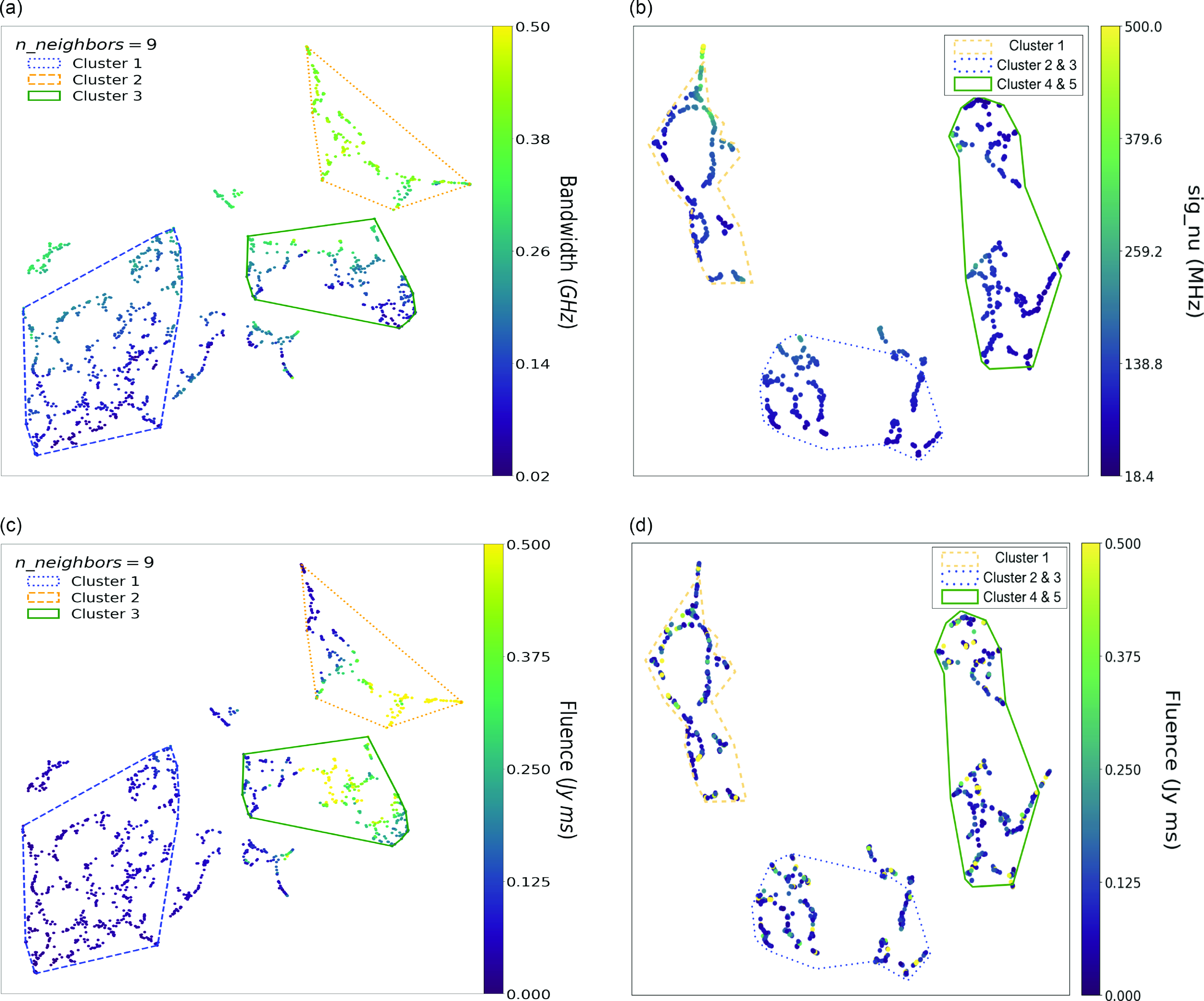
Figure 9. (Left) Classification results from FAST data (Raquel et al. Reference Raquel, Hashimoto, Goto, Chen, Uno, Hsiao, Kim and Ho2023), there are three clusters, Cluster 2 has the highest value of Bandwidth, same as Fluence, Cluster 2 has the higher value in general, and so does Cluster 3. (Right) Classification results from this work. While our result shows that there are five clusters, Fluence looks more uniform in each cluster. As for Bandwidth(sig_nu), same as Cluster 2 in another classification result (Raquel et al. Reference Raquel, Hashimoto, Goto, Chen, Uno, Hsiao, Kim and Ho2023), our Cluster 1 has the highest value in general.
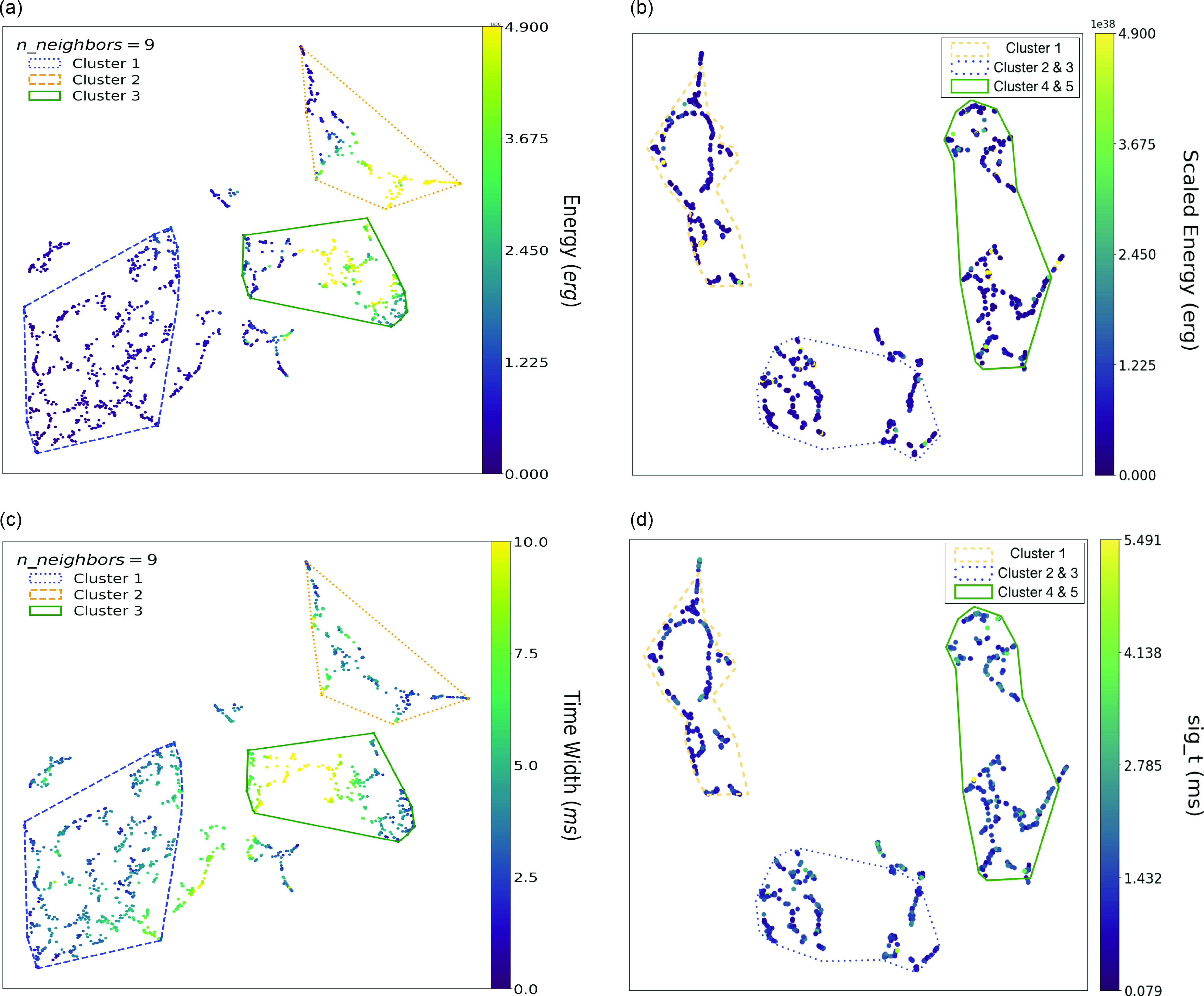
Figure 10. (Left) Classification results from FAST data (Raquel et al. Reference Raquel, Hashimoto, Goto, Chen, Uno, Hsiao, Kim and Ho2023), there are three clusters, both Cluster 2 and Cluster 3 have the higher values of Energy, Cluster 1 has the lowest, most of the data points show most of the values lower than
![]() $1.225\times10^{38}$
erg. On the other hand, Cluster 3 has the longest time width (also duration), most of them are longer than 5.0 ms according to (c). (Right) Classification results from this work. While our result shows that there are five clusters, Scaled Energy looks more uniform to each cluster, however, Cluster 4 and Cluster 5 seem to have higher values of data points. As for Time Duration (sig_t), Cluster 4 and Cluster 5 have the longer time duration, followed by Cluster 2 and Cluster 3.
$1.225\times10^{38}$
erg. On the other hand, Cluster 3 has the longest time width (also duration), most of them are longer than 5.0 ms according to (c). (Right) Classification results from this work. While our result shows that there are five clusters, Scaled Energy looks more uniform to each cluster, however, Cluster 4 and Cluster 5 seem to have higher values of data points. As for Time Duration (sig_t), Cluster 4 and Cluster 5 have the longer time duration, followed by Cluster 2 and Cluster 3.
5.5 Advantage of the machine-learning approach
The classification of Classical and Atypical bursts based solely on the BT might be an arbitrary choice. In contrast, we simultaneously treat seven parameters, which include ones used to compute the BT. This is where the potential advantages of ML come into play. ML models possess the capability to process vast amounts of data and discern complex patterns that may elude human bias. This could potentially lead to a more comprehensive understanding of the classification of FRBs.
Our utilization of UMAP effectively categorized FRBs into five distinct clusters, alongside noise, hinting at the possibility of multiple physical mechanisms responsible for generating FRBs, though not exclusively (Jahns et al. Reference Jahns2022). To mitigate the potential impact of telescope bias, we corroborated our findings with an alternative ML classification method utilizing FAST data (Raquel et al. Reference Raquel, Hashimoto, Goto, Chen, Uno, Hsiao, Kim and Ho2023). The striking alignment between these two approaches provides intriguing insights for future investigations.
While machine learning can significantly reduce human bias in the analysis process, a complete elimination of human bias remains challenging when interpreting and comprehending the results. Nevertheless, machine learning methods tend to introduce far less human bias compared to traditional manual analysis techniques.
6. Conclusions
With the above underpinnings, this paper concludes the following:
-
• Using machine learning classification methods,we identified five clusters among the seven parameters. Each cluster exhibits distinct characteristics in histograms and parameter colouring, which might suggest the existence of multiple mechanisms of FRB emissions. The geometry of the emission region and the propagation effect of FRB signals could also make such distinct clusters.
-
• With parameter colouring,we have determined the invariant properties of each cluster regardless of the n_neighbors value, which demonstrates that describing FRB subtypes without relying on the n_neighbors setting facilitates comparison with other studies aimed at classifying FRBs.
-
• Classifying and confirming the actual physical mechanisms of the clusters in this work are challenging. Consequently, the Critical Temperature criterion may not be applicable to this work.
-
• Nevertheless, a certain degree of agreement with other results (e.g., being able to recover the FRB classification used by Raquel et al. 2023) exhibits consistency and foundation on physical parameters of the clusters.
Looking ahead, we expect even more promising outcomes in the future, thanks to enhanced telescope capabilities provided by future projects like the Square Kilometre Array (SKA) (e.g., Dewdney et al. Reference Dewdney, Hall, Schilizzi and Lazio2009; Hashimoto et al. Reference Hashimoto2020) and the Bustling Universe Radio Survey Telescope in Taiwan (BURSTT) (e.g., Lin et al. Reference Lin2022; Ho et al. Reference Ho, Hashimoto, Goto, Lin, Kim, Uno and Hsiao2023). We maintain optimism that these advancements will unveil the enigmatic nature of FRBs. This research serves as a benchmark for future FRB classifications, particularly as dedicated radio telescopes like SKA and BURSTT continue to detect a growing number of FRBs.
Acknowledgments
We appreciate the referee’s insightful comments, which have greatly enhanced the quality of the manuscript. LL acknowledges the Taiwan Astronomical ObserVatory Alliance (TAOvA) grant NSTC 111-2740-M-008-003 for the summer student internship in partial financial support of this research. The authors would like to express our gratitude to our collaborators in the NTHU & NCHU Cosmology Group, including Yu-Wei Lin, Tzu-Yin Hsu, Poya Wang, Shotaro Yamasaki and many others for their invaluable contributions and support throughout this project. TG acknowledges the support of the National Science and Technology Council of Taiwan through grants 108-2628-M-007-004-MY3, 110-2112-M-005-013-MY3, 112-2112-M-007-013, and 112-2123-M-001-004-. TH acknowledges the support of the National Science and Technology Council of Taiwan through grants 110-2112-M-005-013-MY3, 110-2112-M-007-034-, 113-2112-M-005-009-MY3, and 112-2123-M-001-004-. SH acknowledges the support of The Australian Research Council Centre of Excellence for Gravitational Wave Discovery (OzGrav) and the Australian Research Council Centre of Excellence for All Sky Astrophysics in 3 Dimensions (ASTRO 3D), through project number CE17010000 and CE170100013, respectively. This work is based on observations made with the Arecibo Telescope. The Arecibo Observatory is a facility of the National Science Foundation operated under a cooperative agreement by the University of Central Florida and in alliance with Universidad Ana G. Mendez, and Yang Enterprises.
Data availability statement
The data underlying this article is available in the work of (Jahns et al. Reference Jahns2022). The dataset was derived from https://academic.oup.com/view-large/389045964 and https://academic.oup.com/view-large/389045965. Other data described in this article will be shared upon reasonable request to the corresponding author.
Appendix A. Testing n_neighbors parameters
Here, we present embedding, clustering, and colouring results with different assumptions on n_neighbors values.
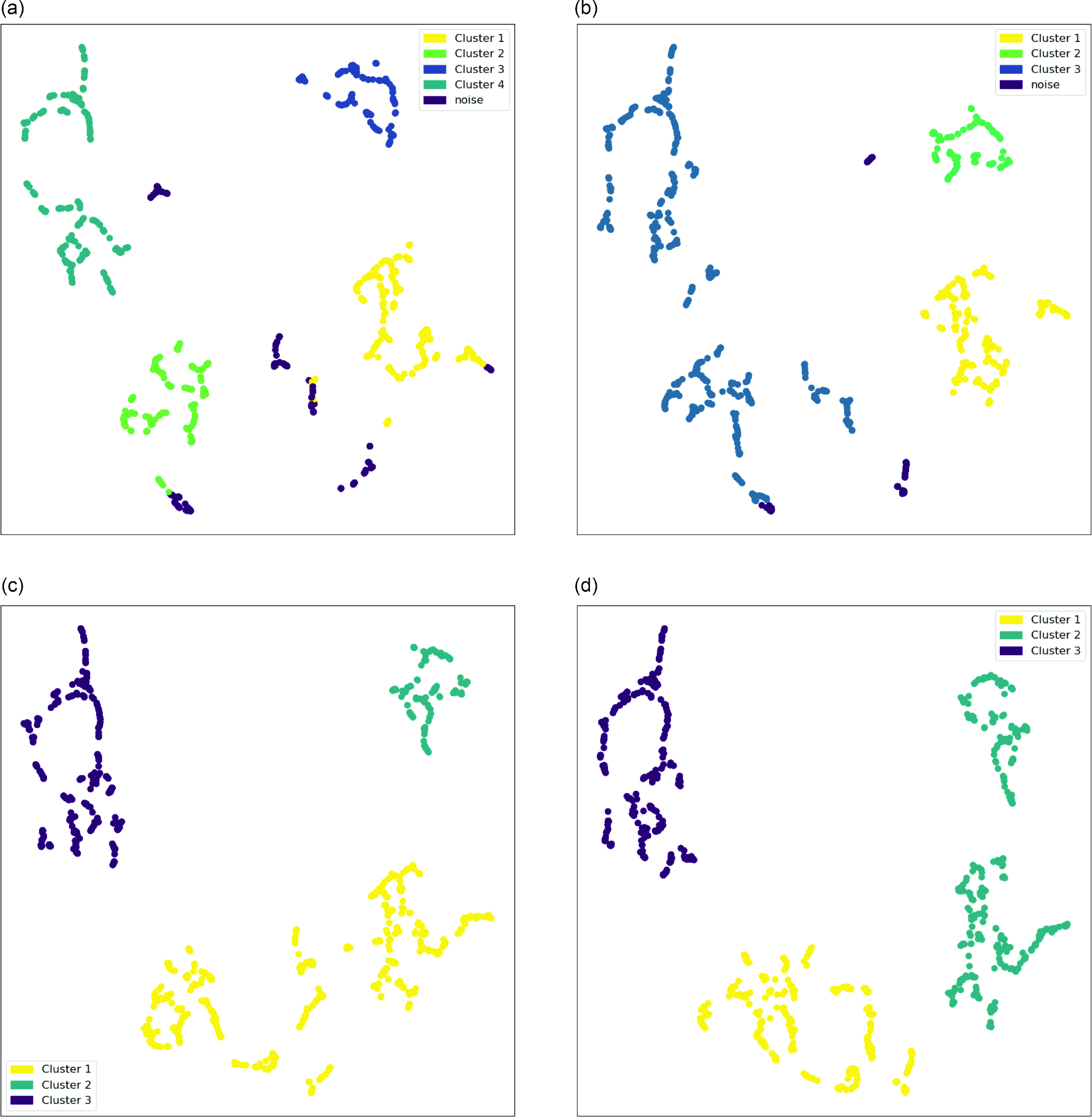
Figure A1. HDBSCAN Clustering result for (a) n_neighbors = 5, (b) n_neighbors = 6, (c) n_neighbors = 7, and (d) n_neighbors = 9.
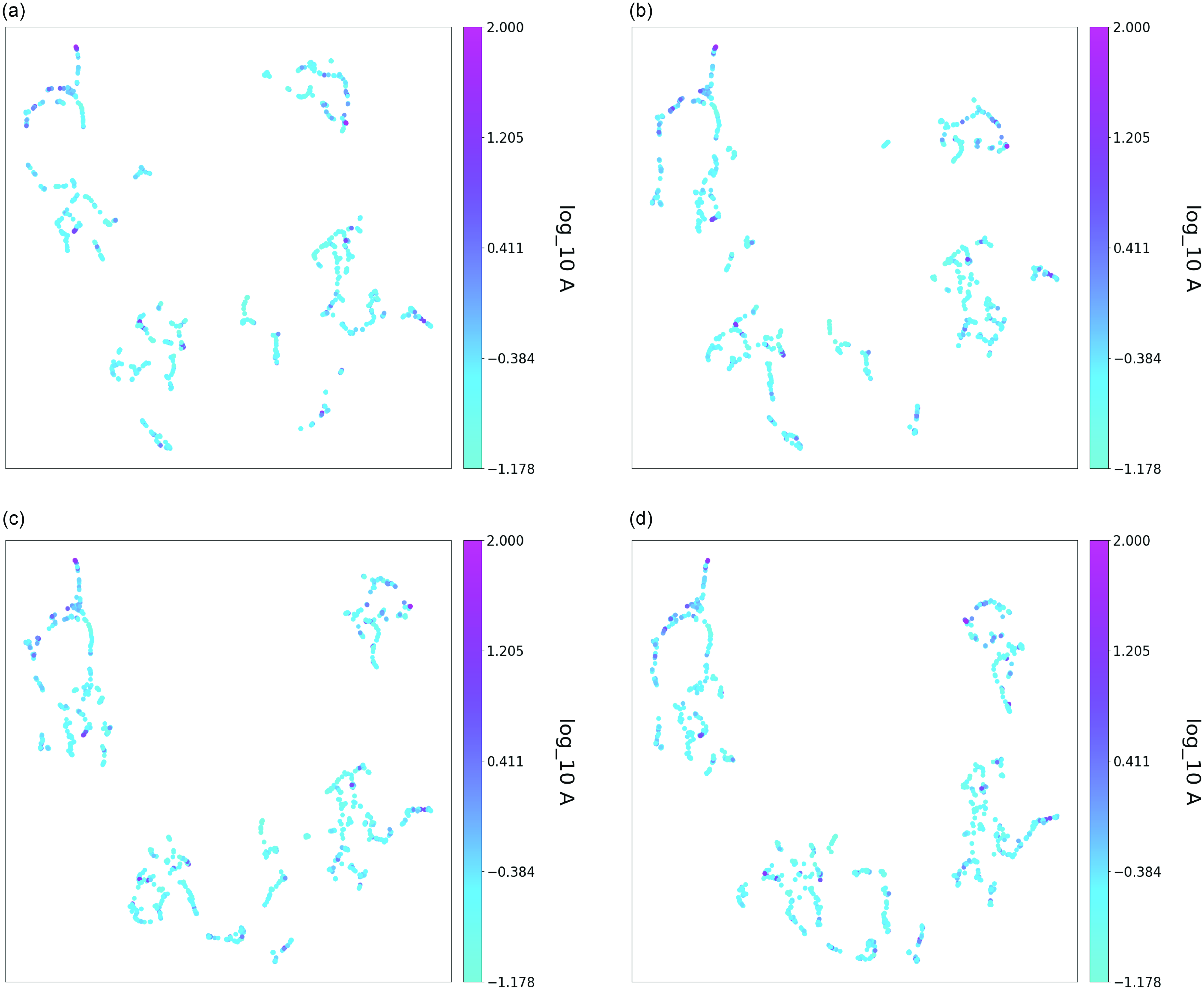
Figure A2. Amplitude colouring of the clustering results for (a) n_neighbors = 5, (b) n_neighbors = 6, (c) n_neighbors = 7, and (d) n_neighbors = 9.
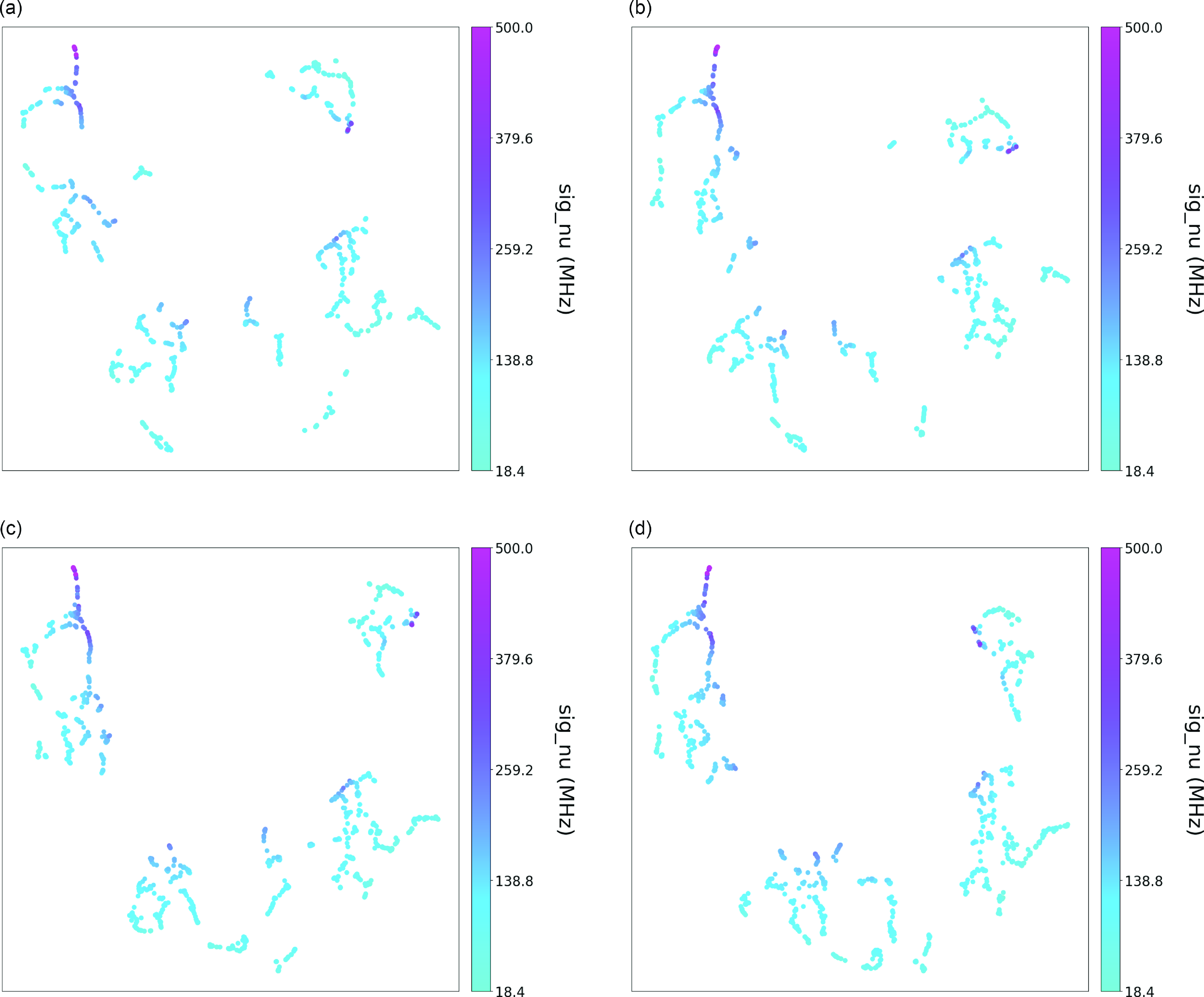
Figure A3. Bandwidth colouring of the clustering results for (a) n_neighbors = 5, (b) n_neighbors = 6, (c) n_neighbors = 7, and (d) n_neighbors = 9.
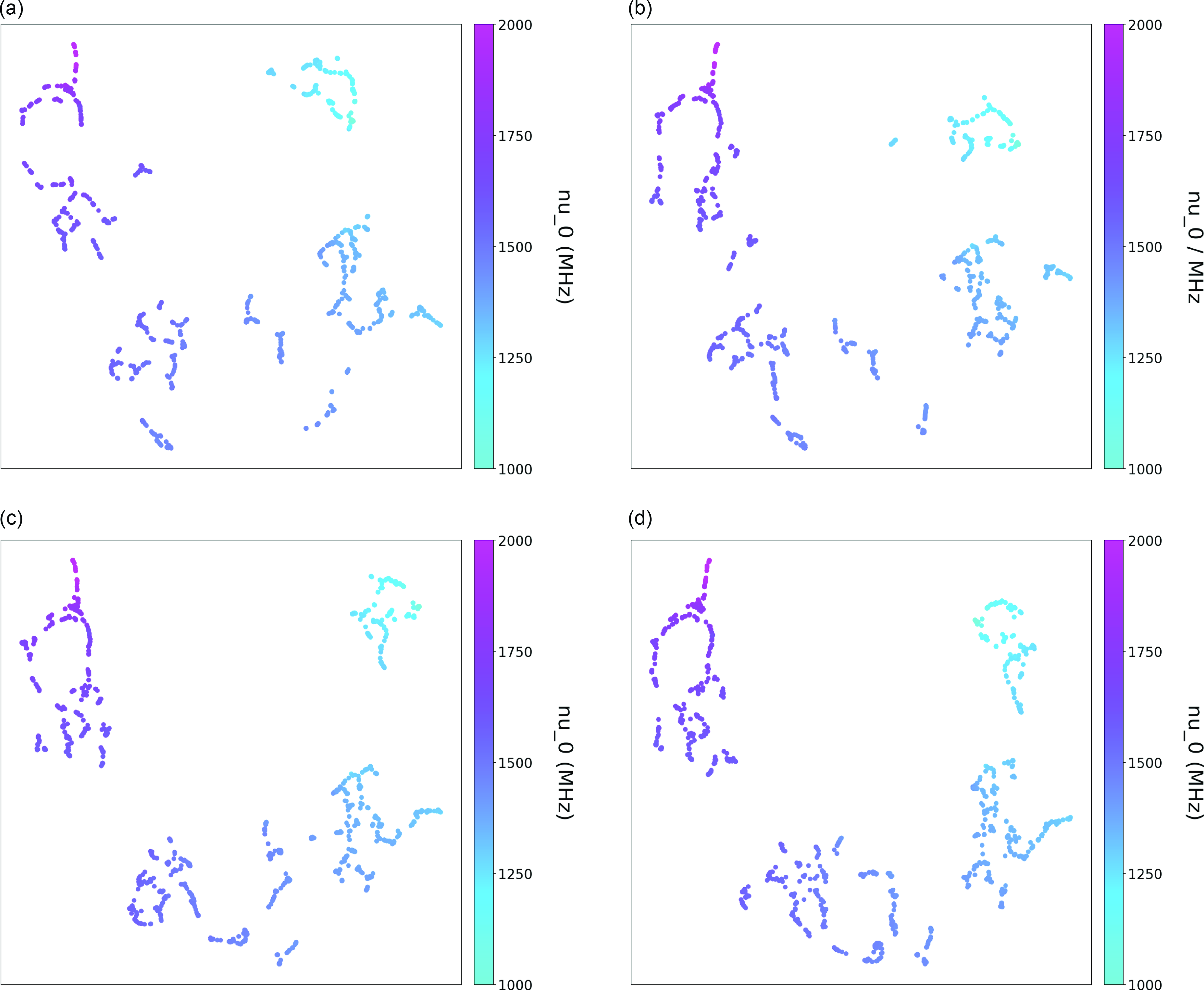
Figure A4. Central Frequency colouring of the clustering results for (a) n_neighbors = 5, (b) n_neighbors = 6, (c) n_neighbors = 7, and (d) n_neighbors = 9.
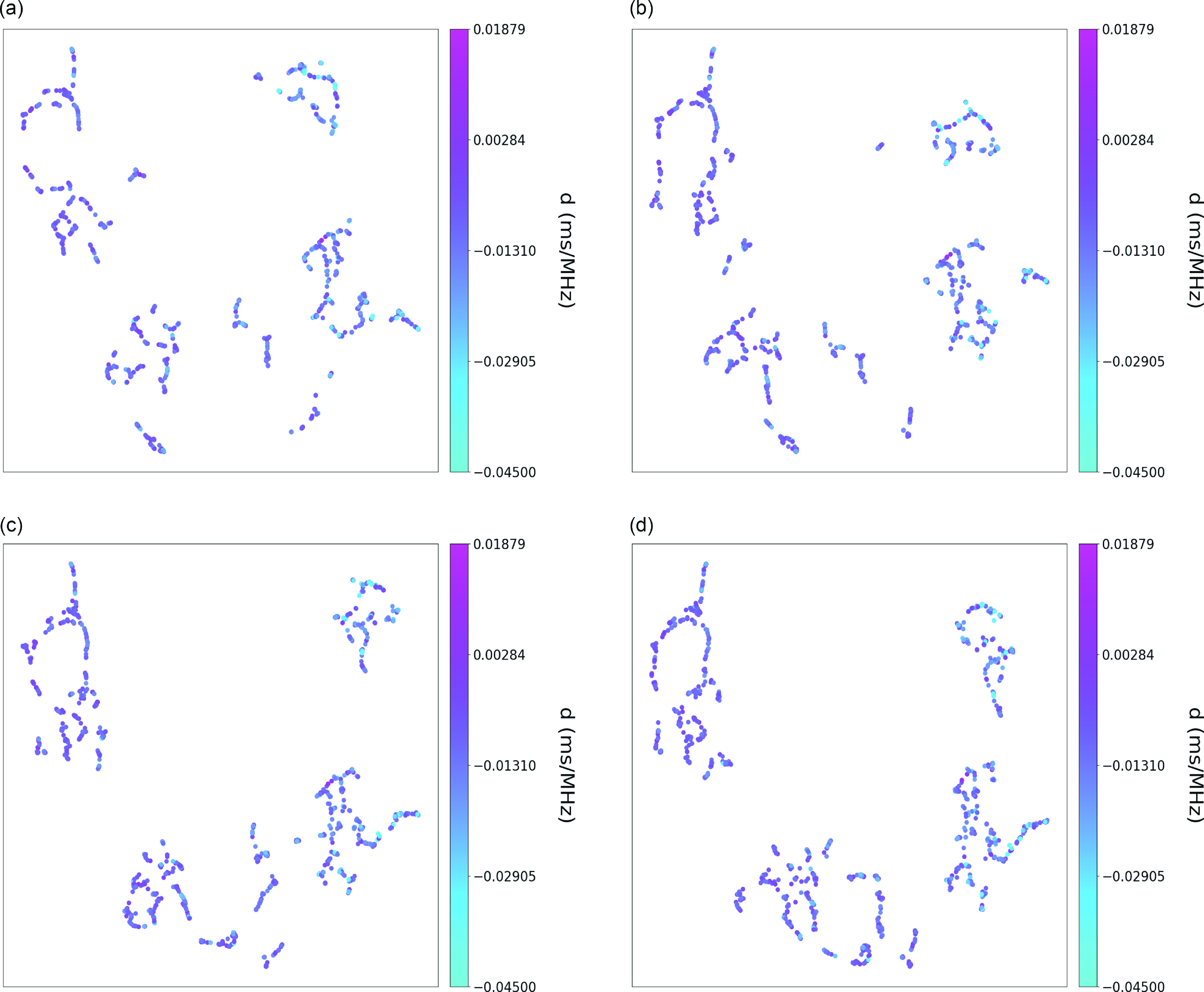
Figure A5. Linear Temporal Drift colouring of the clustering results for (a) n_neighbors = 5, (b) n_neighbors = 6, (c) n_neighbors = 7, and (d) n_neighbors = 9.
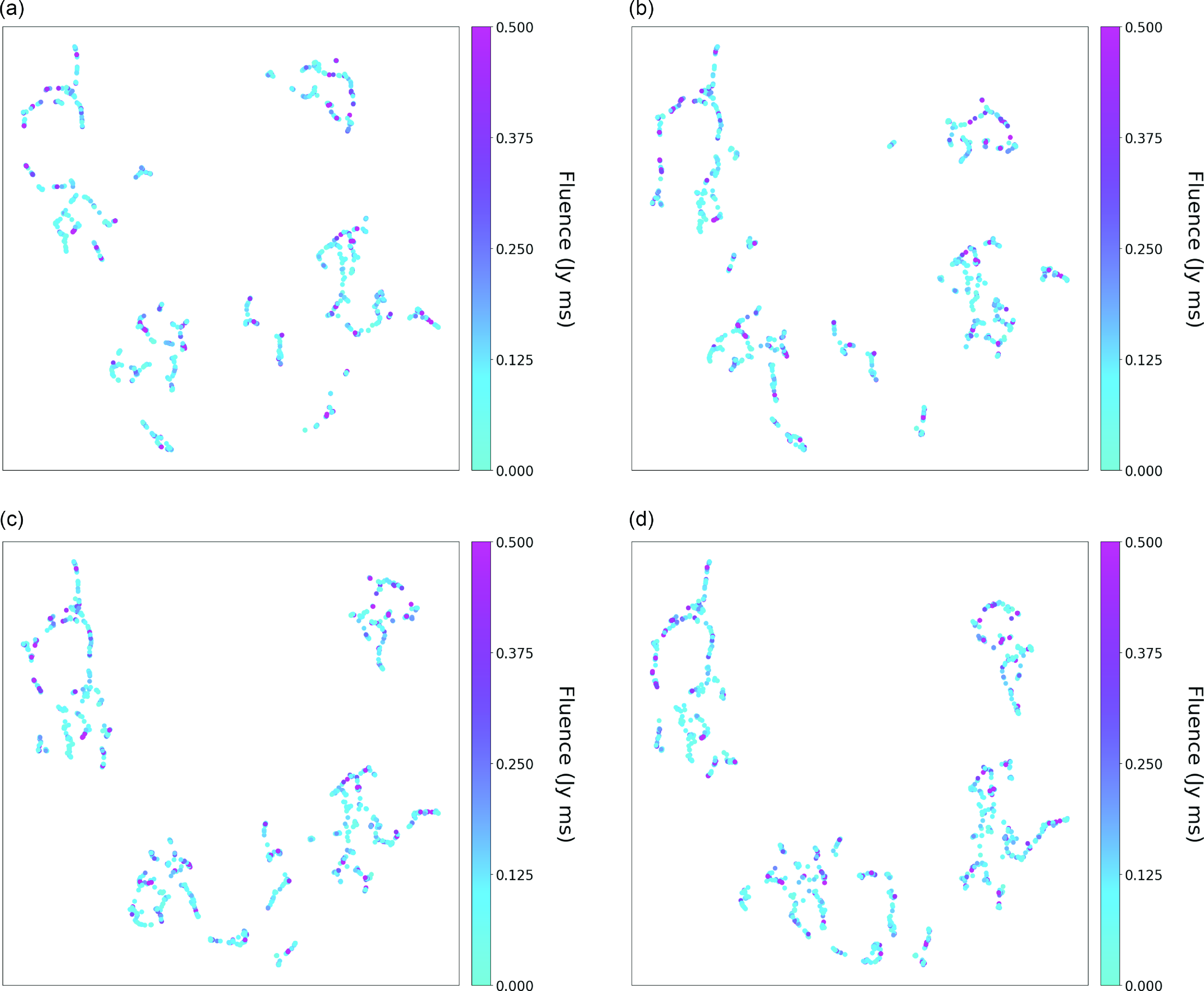
Figure A6. Fluence colouring of the clustering results for (a) n_neighbors = 5, (b) n_neighbors = 6, (c) n_neighbors = 7, and (d) n_neighbors = 9.
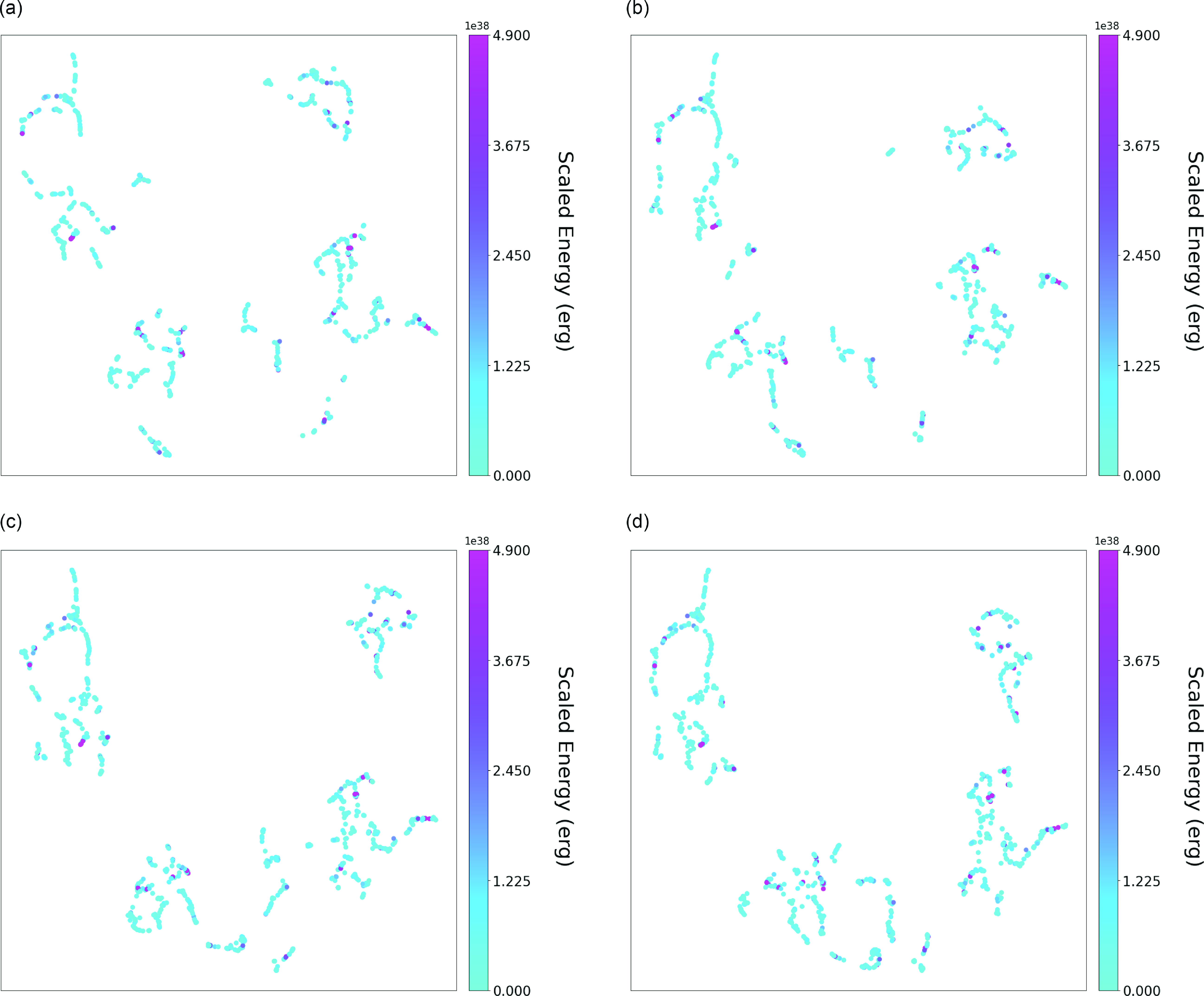
Figure A7. Scaled Energy colouring of the clustering results for (a) n_neighbors = 5, (b) n_neighbors = 6, (c) n_neighbors = 7, and (d) n_neighbors = 9.

Figure A8. Time Duration colouring of the clustering results for (a) n_neighbors = 5, (b) n_neighbors = 6, (c) n_neighbors = 7, and (d) n_neighbors = 9.
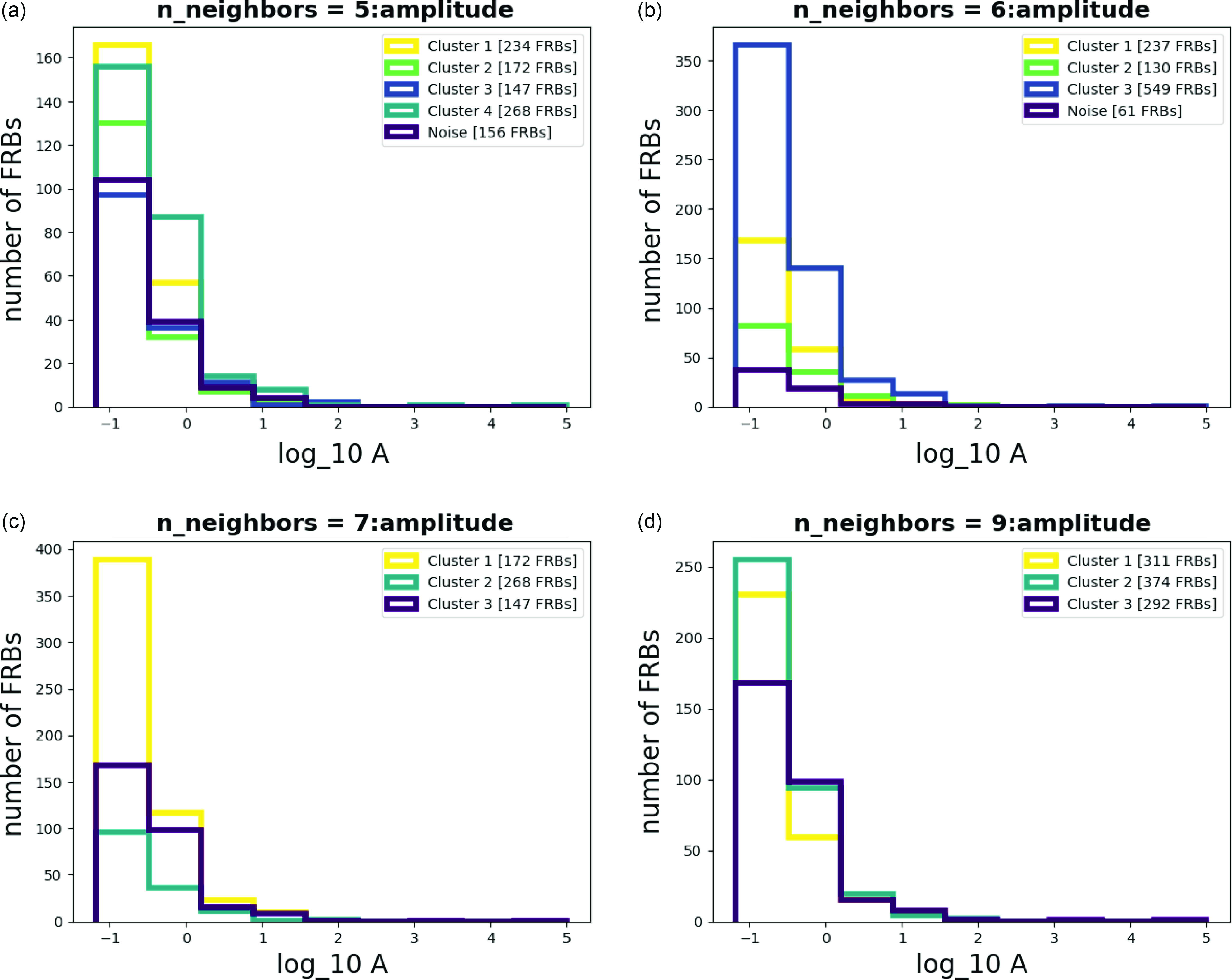
Figure A9. Histograms for Amplitude with different n_neighbors.
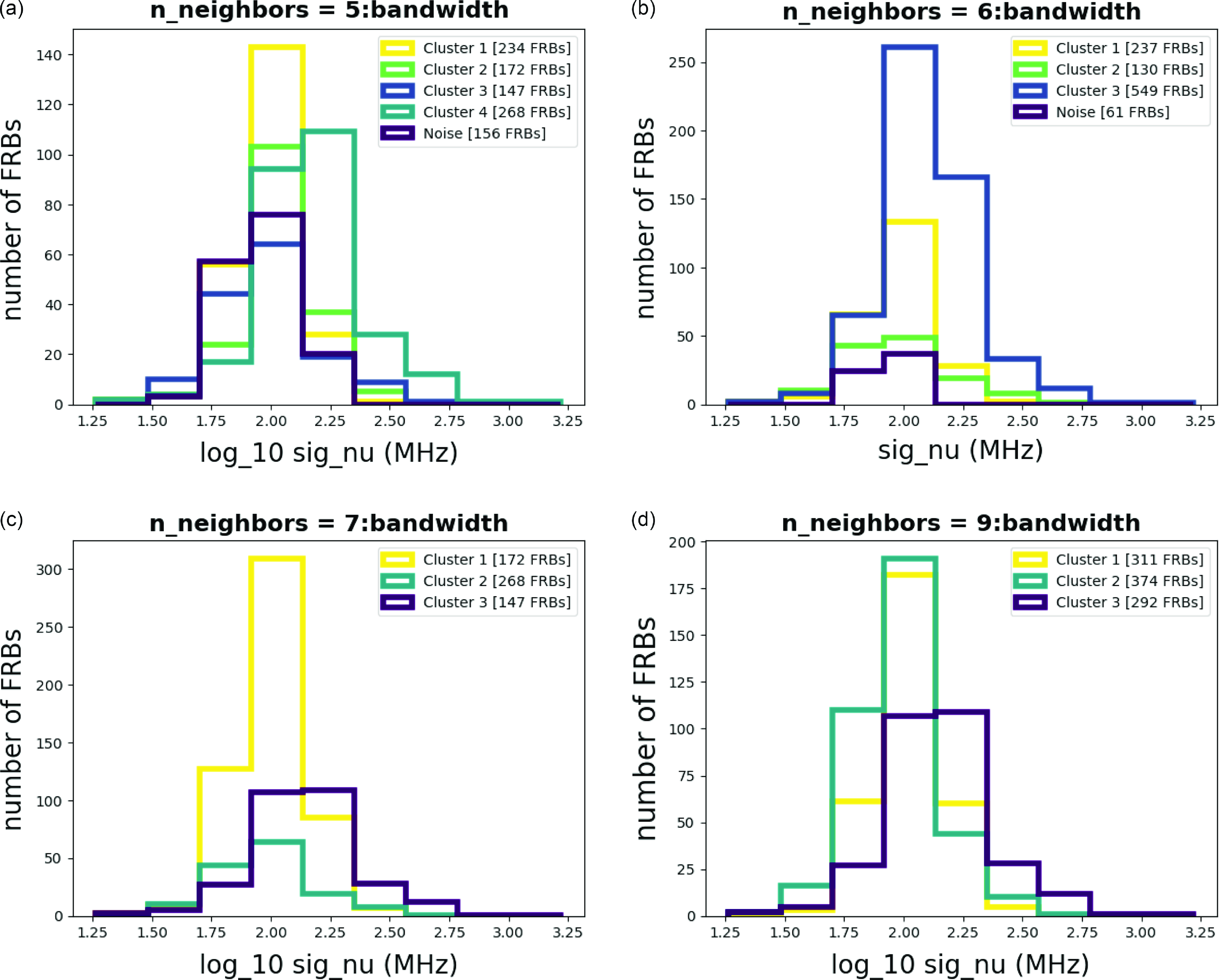
Figure A10. Histograms for Bandwidth with different n_neighbors.

Figure A11. Histograms for Central frequency with different n_neighbors.
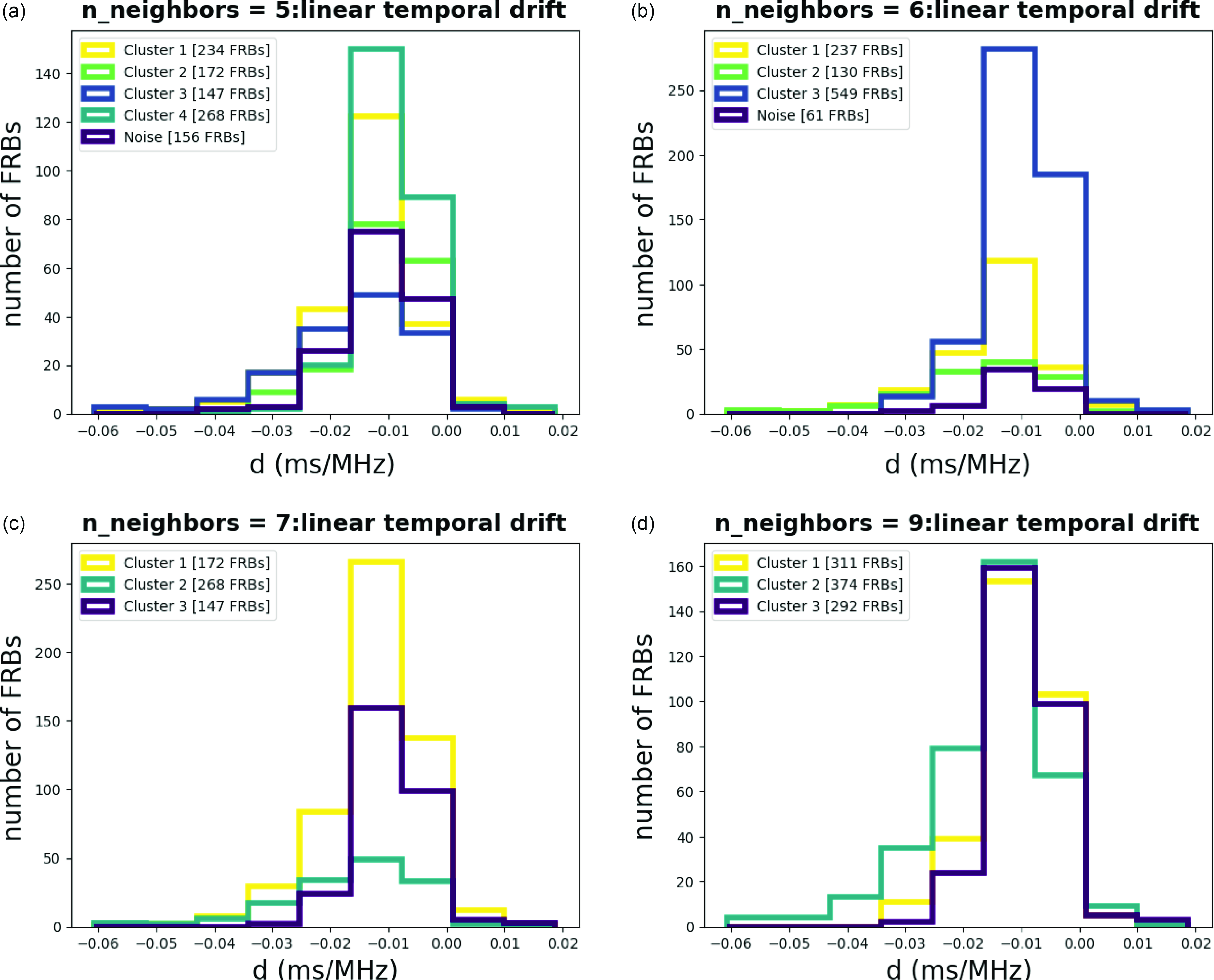
Figure A12. Histograms for Linear temporal drift with different n_neighbors.
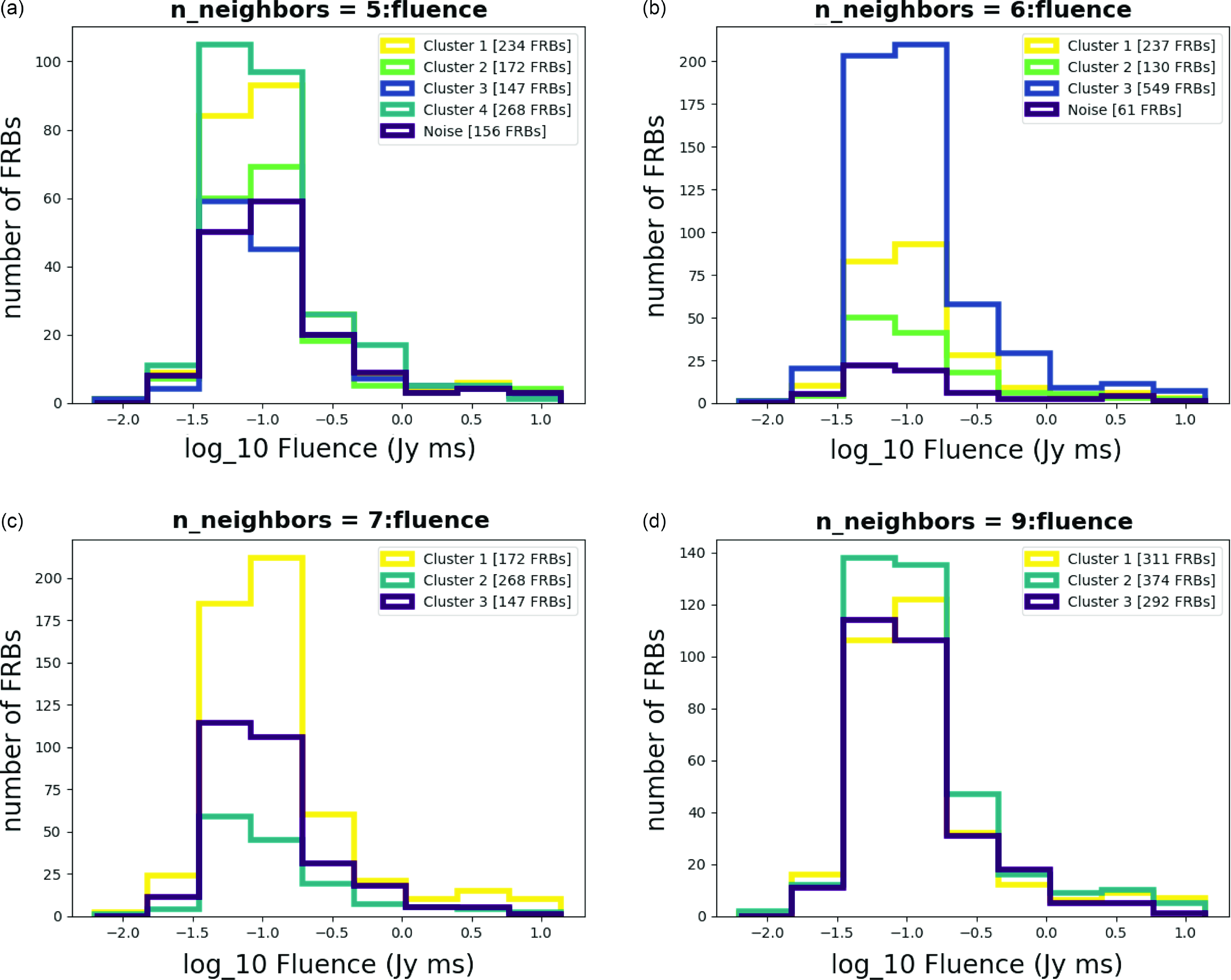
Figure A13. Histograms for Fluence with different n_neighbors.

Figure A14. Histograms for Scaled energy with different n_neighbors.
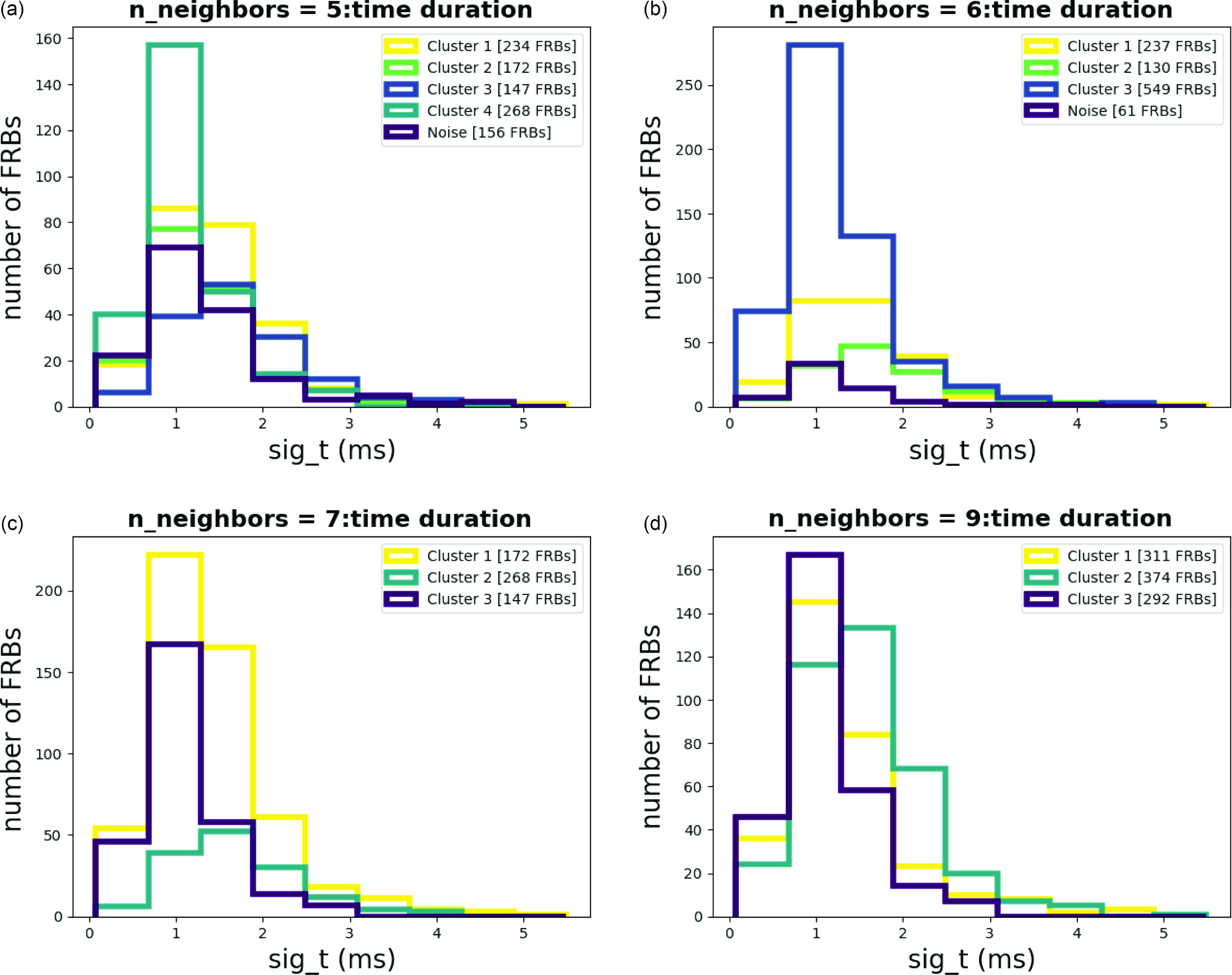
Figure A15. Histograms for Time duration with different n_neighbors.


