Foreign financial shocks and domestic credit policy in the small open economy

Abstract

This paper introduces a global banking system in a small open economy DSGE model and features global relative price adjustments with incomplete asset market to investigate the role of international financial imperfections. We show that credit policy could be more powerful than monetary policy to alleviate foreign financial shocks since an expansionary monetary policy and alternative policy rules are not a sufficient tool in the global financial crisis. In particular, credit policy based on international credit spread outperforms credit policy based on domestic credit spread since the former attempts to remove distortions from international financial imperfections and reduces real costs of foreign loans. Accordingly, the lower costs of external finance further boost investment and effectively stabilize the economy without substantial asset purchases.

1. Introduction

The global financial crisis featured significant disruption of financial intermediaries and cross-border spillovers. The meltdown of the shadow banking system due to the collapse of the U.S. housing market bubble and loose regulatory policies deteriorated the entire financial system and the world economy. Thus, a new generation of DSGE models incorporate frictions in financial intermediaries ¹ such as Cúrdia and Woodford (2016), Gertler and Karadi (2011), Gertler and Kiyotaki (2010, 2015), Gertler et al. (2012), Gertler et al. (2020) and Akinci & Queralto (2022).

In order to capture cross-border capital flows through the banking sector across countries and to evaluate the role of international financial imperfections, the model in this paper introduces a global banking system into a small open economy DSGE model and analyses how the source of funds (deposits and global bank loans) changes in response to financial shocks. We construct a microfounded two-country model to fully investigate the transmission mechanism of foreign shocks on the small open economy through international risk sharing, global banking and trade channels. While depreciation of the exchange rate raises net exports, it also raises the real interest rates and lowers consumption through risk sharing conditions. Also, the balance sheet of domestic banks shrinks due to debts denominated in foreign currency from the global banks, making the economy more vulnerable. In a closed economy DSGE model with financial frictions, where banks are constrained in obtaining funds from households, a financial crisis affects the economy through a financial accelerator mechanism. We identify that in our open economy model, global bank loans and risk sharing conditions generate additional financial channels. In particular, domestic banks in the small open economy can obtain additional funds from global banks and this in turn, exposes to the risk of capital flights and the currency risk, which influence the balance sheet of domestic banks.

Since small open economies are vulnerable to global financial and nonfinancial conditions, our model embeds small open economy features in a tractable way. The response of the terms of trade and the real exchange rate allows us to investigate changes in trade and the current account. Also, allowing different degree of trade openness and banking system stability offers sources of heterogeneous dynamics of small open economies. A distinctive feature is that our model embeds an incomplete asset market structure in line with empirical evidence on the lack of risk sharing (i.e the Backus and Smith (1993) puzzle) ² in terms of both international government bonds and the global bank loans market thereby allowing imperfect risk sharing in consumption and making explicit international links between the real interest rate, the real exchange rate and consumption. In other words, this model makes it possible to explore the role of international financial imperfections, and the transmission mechanism of foreign shocks and policies in a way consistent with empirical grounds.

We document the effects of foreign financial shocks and then, look at the role of credit policy based on domestic and international credit spread, an expansionary monetary policy, ³ and alternative monetary policy rules to combat the financial crisis. Two main findings stand out. Firstly, foreign financial shocks capture cross-border spillovers in the small open economy through the global banking system. In particular, the shocks broadly mimic a global financial crisis in the small open economy as defined by Calvo et al. (2006), Mendoza (2010) and Gourinchas and Obstfeld (2012): (a) contractions of output and investment, (b) decline in the net worth and asset prices, (c) a fall in CPI inflation, (d) reversals of international capital flows in terms of an increase in net exports and drops of global bank loans, (e) a depreciation of the terms of trade and the real exchange rate. Also, we show that country differences in the severity of the shocks depend on the degree of trade openness and banking system stability.

Secondly, while credit policy is powerful in response to foreign financial shocks by injecting credit flows to intermediate firms, the expansionary monetary policy and alternative monetary policy rules are not sufficient to alleviate the global financial crisis. We find that among alternative monetary policy rules, the Taylor rules with international credit spread which refers to the spread between the return on domestic private assets and international borrowing costs of domestic banks, outperform the Taylor rules with output, real exchange rate and markup. In particular, credit policy based on international credit spread formed by international financial imperfections outperforms credit policy based on domestic credit spread since the latter leads to “excess smoothness” in the exchange rate and interrupts a role of the real exchange rate as a foreign financial shock absorber. On the other hand, a feedback rule with international credit spread attempts to remove distortions from international financial imperfections, allows a fall in global bank interest rate and an appreciation of the real exchange rate, and thus reduces the real cost of global bank loans. This in turn, increases investment, price of assets, consumption and output further. The global banking channel dominates a trade channel which reduces net exports and output in response to the appreciation. This implies that international financial imperfections play a major role in monetary and credit policies in an open economy.

1.1. Literature

There have been many attempts to incorporate incomplete international asset markets with and without financial intermediaries in an open economy framework. Gabaix and Maggiori (2015) and Itskhoki and Mukhin (2021) among others provide a theory of the determination of exchange rates in imperfect financial markets where financiers having limited risk bearing capacity require a risk premium for holding currency risk, resulting in deviations from the uncovered interest parity. Maggiori (2017) embeds an international market for interbank loans and asymmetric financial development across countries, and thereby allowing imperfect risk sharing in consumption. Kollmann et al. (2011) and Dedola et al. (2013) show how country specific shocks lead to financial and macroeconomic interconnections across countries. However, in order to examine two large countries, the literature assumes a symmetric two country framework and does not embed important features of the open economy such as global relative prices (the terms of trade and the real exchange rate) and incomplete asset market structure. In addition, they analyze cross-border capital flows between banks and non-banks and thus they do not embed a global banking system: banks lend funds to both domestic and foreign firms but banks in one country do not lend to banks in another country. However, as shown in Kalemli-Ozcan et al. (2013) and Bruno and Shin (2014), cross-border capital flows through the global banking system account for a large proportion of total cross-border debt flows ⁴ and they are a critical determinant of macroeconomic synchronization. Global bank loans significantly alter the balance sheets of domestic banks, which boost the economy by lending more funds to domestic firms in normal times but trigger a financial crisis by suddenly withdrawing loans. This paper is also related to Banerjee et al. (2016) and Devereux et al. (2020). These papers analyze the optimal policy and the role of international financial intermediaries in a two country model with asymmetric size of the economies and shows that monetary policy needs to take account financially integrated economies. However, they characterize the optimal policy or the optimal policy rules with fixed target coefficients rather than interest rules. Also, they do not embed credit policy and international financial imperfections (i.e., deviations from the uncovered interest parity for both international bond markets and global banking sectors), thereby excluding explicit linkages between the returns of international assets. Aoki et al. (2016) develops a small open economy model with financial intermediaries and analyses the transmission mechanism of foreign (interest rate) shocks through the fluctuation of the real exchange rate. In contrast to Aoki et al. (2016), we formulate a microfounded two-country structure and compare the effectiveness of monetary and credit policies. In particular, this paper embeds international financial imperfections to explore intrinsically different nature of monetary and credit policies in an open economy from those in a closed economy. Akinci and Queralto (2022) provides a small open economy extension of the macroeconomic model with financial intermediaries and occasionally binding constraint. They find that macro-prudential policy providing subsidy to equity issuance can effectively reduce a risk of crisis.

Also, extensive studies have accessed the role of foreign financial developments on domestic economy. The literature shows that international goods and financial markets are highly integrated due mainly to an international credit channel. Cesa-Bianchi et al. (2018) construct a small open economy model of collateralized borrowing within housing markets and show that an increase in international credit supply leads to an excessive housing price developments, subject to the loan to value ratio and the share of foreign currency denominated credit. Also, Bergant et al. (2024) and Coman and Lloyd (2022) implement empirical analysis and find that the effects of foreign shocks to emerging economies can be partially offset by tighter macro-prudential regulations. Alpanda and Kabaca (2020) construct an estimated two-country model with long-term bonds and investigate the international spillover effects of large-scale asset purchases in the United State on the rest of the world. They find that the purchases lead to capital inflows in the rest of the world, thereby reducing the long-term bonds interest rate and stimulating the economy. Bhattarai et al. (2021) find that while the purchases in the United State reduce the long-term bonds interest rate, they do not find consistent and significant effects on output in emerging market economies using a Bayesian panel VAR. Wu et al. (2024) show that foreign shocks can be amplified as the duration of long-term bonds increases. The longer the duration of the bond, the greater the exchange rate volatility, influencing more on net exports, investments and output. The contribution of this paper is that it presents an appropriately-augmented theoretic framework by embedding global banking system, international financial imperfections and global relative price adjustments to assess a range of policies and financial shocks. In particular, by imposing a fully microfounded structure of foreign country, our model allows to investigate the effects of foreign financial and nonfinancial shocks on a small open economy through both trade and financial channels.

The paper is organized as follows: Section 2 describes the key macroeconomic variables in the global financial crisis. In Section 3, we describe the model including the incomplete asset market structure and the global banking system. Section 4 presents quantitative results. We analysis the impact of disturbances to the small open economy and the large economy to the agency cost and show how the disturbances in both economies could influence the small open economy. Then, we evaluate the extent to which credit policy, the expansionary monetary policy and alternative monetary policy rules to alleviate the financial crisis. Finally, our concluding remarks are presented in section 5.

2. Stylised facts of the global financial crisis

Figure 1. U.S., Korea and Canada.

Note: While the nominal interest rate (overnight call rate (Korea and Canada) and effective federal funds rate (U.S.)) and international credit spread (between Libor and the yields on AA rated corporate bonds for Korea (the business prime rate for Canada)) are the annualized, other variables are expressed in log de-trended and estimated from 1994q4 to 2014q3. Following Christiano et al. (2011), stock prices (stock price index (Korea and Canada) and Dow Jones index (U.S.)), scaled by the GDP deflator are included. An increase in the real effective exchange rate indicates depreciation of the Korean and Canadian currencies against a broad basket of currencies. Source: The Bank of Korea, Statistics Canada, Federal Reserve Economic Data and BIS Statistics (Consolidated banking statistics).

Our primary focus is on the experience of small open economies spilled over from a global financial crisis so that we show main US, Korean and Canadian variables during 2008q3–2012q3 in Figure 1. South Korea and Canada have the world’s most open goods and financial markets and thus they can be exposed to volatile capital flows and foreign currency risk. South Korea and Canada are small open economies which are unlikely to influence the foreign interest rate, output and prices. Also, since two economies have different degree of trade openness and banking system stability, ⁵ the movement comparison of main macroeconomic variables in different countries offers sources of heterogeneous dynamics of each economy in the global financial crisis.

Financial liberalization, started in the 1990s relaxed restrictions on foreign loans and entry of financial institution and led to a substantial increase in cross-border borrowing from global banks, largely in the form of short-term debt. The stock of consolidated claims of global banks on both Korea and Canada accounted for about $30\%$ of GDP in 2008q3. The global financial crisis started in the US and featured significant disruption of financial intermediaries and the global banking system. A depreciation of the real exchange rate raised the real cost of global bank loans and confidence of global banks was rapidly eroded in the financial crisis. Thus, Korean and Canadian banks were unable to roll over their short-term debt and foreign capital suddenly outflowed. Also, the banks attempted to reduce leverage by selling their assets and reducing loans to firms. The international credit spread sharply increased during the first two quarters, raising the cost of capital and this in turn reduced investment and output. Correspondingly, real GDP, consumption, CPI inflation, investment and the claims of global banks decreased. While the Canadian economy has a more stable banking system, the economy has more open goods markets so that lower foreign demand for Canadian goods coupled with lower price of imports reduced CPI inflation further and generated a symmetric fall in output. In order to recover the economy, the central banks of the small open economies aggressively reduced the nominal interest rate. Over the period given, variables show strong positive inter-country correlation.

3. Model

We develop a small open economy DSGE model with international financial imperfections and a global banking system. The baseline framework follows Benigno and Benigno (2003), Gali and Monacelli (2005), Benigno (2009), Gertler and Kiyotaki (2010, 2015) and Gertler and Karadi (2011). We extend the baseline DSGE model by embedding an incomplete asset market structure in the model presented in subsection 3.1–3.3 and introducing the global banking system between domestic and global banks presented in subsection 3.4.

3.1. Households

The world is composed of two countries, the “home” and the “foreign” country labeled by f. Households on the subinterval [0, n] live in the home country and households on the subinterval [n, 1] live in the foreign country. Since we assume that the home country is a small economy that is unable to influence the foreign economy, the foreign economy is analogous to a closed economy.

Each domestic household contains a large number of individuals. It supplies labor, makes deposits in domestic banks, and holds both domestic currency denominated bonds and foreign currency denominated bonds. Domestic government bonds and deposits in domestic banks are perfect substitutes. Following Gertler and Karadi (2011), within the household, a fraction 1-e of individuals are workers and a fraction e are bankers. While workers supply labor and earn wages, bankers manage the bank and transfer bank dividends to the household. Each household consumes final goods from domestic and foreign countries, and consumption risk is perfectly pooled within the household.

The intertemporal utility of a representative household in the home economy is given by

(1) \begin{align} \sum _{t=0}^{\infty } \beta ^t U(C_t,L_t) \end{align}

where per-period utility is

(2) \begin{align} U(C_t,L_t)=\dfrac {(C_{t}-hC_{t-1})^{\tiny {1-\rho }}}{1-\rho } -\Re \dfrac {L_{t}^{1+\varphi }}{1+\varphi } \end{align}

where $ \rho$ is the coefficient of relative risk aversion, $h$ is the habit persistence parameter and $ \varphi$ is the inverse of the Frisch elasticity of labor supply. Aggregate consumption of a representative home (foreign) household is given by

(3) \begin{align} {\textrm{C}}_{\textrm{t}} & = \left [{\lambda }^{\frac {{ 1}}{\eta }}{({\textrm{C}}_{\textrm{h,t}})}^{\frac {\eta { -1}}{\eta }}{ +}{{ (1-}\lambda )}^{\frac {{ 1}}{\eta }}{({\textrm{C}}_{\textrm{f,t}})}^{\frac {\eta { -1}}{\eta }}\right ]^{\frac {\eta }{\eta { -1}}} ; \nonumber\\ {\textrm{C}}^{\textrm{f}}_{\textrm{t}} &= \left [{{\lambda }^f}^{\frac {{ 1}}{{\eta }^f }}{\left({\textrm{C}}^{\textrm{f}}_{\textrm{f,t}}\right)}^{\frac {{\eta }^f { -1}}{{\eta }^f }}{ +}{{ (1-}{\lambda }^f)}^{\frac {{ 1}}{{\eta }^f }}{\left({\textrm{C}}^{\textrm{f}}_{\textrm{h,t}}\right)}^{\frac {{\eta }^f { -1}}{{\eta }^f }}\right ]^{\frac {{\eta }^f }{\eta { -1}}} \end{align}

where $C_{h,t}$ ( $C^{f}_{f,t}$ ) is the consumption of home (foreign) tradable goods and $C_{f,t}$ ( $C^{f}_{h,t}$ ) is the consumption of foreign (home) tradable goods. Households have a “home bias” that implies, ceteris paribus, that they prefer to consume domestically produced goods. Following Sutherland (2005), $(1-\lambda )=\alpha (1-n)$ is the weight on imported goods, reflecting the relative size of home country $n$ and the degree of openness $\alpha$ . Since a small open economy is characterized by $n\rightarrow 0$ , $(1-\alpha )$ represents the degree of home bias in preferences. $\eta$ ( $\eta ^{f}$ ) is the elasticity of substitution between home tradable goods and foreign tradable goods. For simplicity, we assume the same elasticity of substitution between different varieties across countries. The foreign weight on imports is defined as $(1-\lambda ^{f})=n\alpha$ .

We assume producer currency pricing so that the law of one price holds: $P_{f,t}=X_{t}P_{f,t}^{f}$ and $P_{h,t}=X_{t}P_{h,t}^{f}$ where $P_{f,t}$ ( $P_{h,t}$ ) is the price of imports (domestic goods) denominated in home currency, $X_{t}$ is the nominal exchange rate and $P_{f,t}^{f}$ ( $P_{h,t}^{f}$ ) is the price of foreign goods (exports) denominated in foreign currency.

The optimal allocation of consumption between different countries yields the demand functions

(4) \begin{align} C_{h,t} & = \lambda \!\left(\dfrac {P_{h,t}}{P_{t}} \right)^{\!-\eta }\!C_{t};\;\;\;\;\;\; C_{f,t}=(1-\lambda )\!\left(\dfrac {P_{f,t}}{P_{t}} \right)^{\!-\eta }\!C_{t} \\[-2pt] \nonumber \end{align}

(5) \begin{align} C_{f,t}^{f} & = \lambda ^{f}\!\left(\dfrac {P_{f,t}^{f}}{P_{t}^{f}} \right)^{\!-\eta }\!C_{t}^{f};\;\;\;\;\;\; C_{h,t}^{f}=(1-\lambda ^{f})\!\left(\dfrac {P_{h,t}^{f}}{P_{t}^{f}} \right)^{-\eta }C_{t}^{f} \\[6pt] \nonumber \end{align}

The consumer price index (CPI) corresponding to the aggregate consumption in home and foreign country is given by

(6) \begin{align} {{\textrm{P}}_{\textrm{t}}{ =}\left [\lambda {({\textrm{P}}_{\textrm{h,t}})}^{{ 1-}\eta }{ +(1-}\lambda ){({\textrm{P}}_{\textrm{f,t}})}^{{ 1-}\eta }\right ]}^{\frac {{ 1}}{{ 1-}\eta }} ;\;\ {{\textrm{P}}^{\textrm{f}}_{\textrm{t}}{ =}\left [{\lambda }^f{\left({\textrm{P}}^{\textrm{f}}_{\textrm{f,t}}\right)}^{{ 1-}\eta }{ +(1-}{\lambda }^f){ \left({\textrm{P}}^{\textrm{f}}_{\textrm{h,t}} \right)}^{{ 1-}\eta }\right ]}^{\frac {{ 1}}{{ 1-}\eta }} \end{align}

The household deposits funds in domestic banks and holds domestic and foreign government bonds. These are risk-free assets with a one-period maturity. For simplicity, we assume that while foreign government bonds are traded in both countries, domestic government bonds can only be traded in the domestic country so that foreign households cannot hold domestic government bonds.

Following Schmitt-Grohé and Uribe (2003) and Benigno (2009) who introduce an incomplete asset market structure by limiting cross-border asset borrowing/saving when trading in a single non-state-contingent bond (as opposed to there being a full set of Arrow–Debreu securities), our model embeds an incomplete asset market in the form of bond transaction costs. ⁶ Transactions in foreign currency denominated bonds issued by the foreign government, generate quadratic costs for the foreign government; specifically, quadratic costs are incurred from changing their assets away from the steady state. The foreign government pays these transaction costs to domestic households. The parameter $\tau$ measures the strength of these transaction costs. Thus, the real budget constraint of the representative domestic household is given by

(7) \begin{align} \begin{split} B_{t+1} + D_{t+1} + Q_{t}B_{f,t+1}=& W_{t}L_{t} + \Pi _{t} - T_{t} + R_{t-1}B_{t} + R_{t-1}D_{t} + \\ & Q_{t}R_{t-1}^{f}B_{f,t} + \dfrac {\tau {Q_{t}}}{2}\left(B_{f,t+1} - {B_{f}}\right)^{2} - C_{t} \end{split} \end{align}

The LHS of this expression reflects the real value of domestic government bonds, $B_{t+1}$ , real deposits, $D_{t+1}$ , and the real value (in terms of domestic currency) of foreign government bonds held by domestic households, $Q_{t}B_{f,t+1}$ , where $Q_{t}$ is the real exchange rate. Since both domestic government bonds and deposits are one-period real riskless assets, they are perfect substitutes and pay the same gross real return, $R_{t-1}$ from t-1 to t. The RHS reflects real labor income, $W_{t}L_{t}$ , net profits from the ownership of bank, retail and capital producing firms, $\Pi _{t}$ , lump sum taxes, $T_{t}$ , the gross real interest from holdings of assets, transaction benefits arising from trade in foreign government bonds and consumption.

The corresponding budget constraint for the foreign representative household is

(8) \begin{align} {B_{f,t+1}^{f} + D_{t+1}^{f} = W_{t}^{f}L_{t}^{f} + \Pi _{t}^{f} - T_{t}^{f} + R_{t-1}^{f}B_{f,t}^{f} + R_{t-1}^{f}D_{t}^{f} - C_{t}^{f}} \end{align}

where $B_{f,t+1}^{f}$ are foreign government bonds held by foreign households and denominated in foreign currency.

The optimal domestic households’ decision in terms of deposits, foreign government bonds and labor supply yields the first order conditions

(9) \begin{align} E_{t}\beta \!\left(\dfrac {\nu _{t+1}}{\nu _{t}} \right)\!R_{t} & = 1 \\[-4pt] \nonumber \end{align}

(10) \begin{align} R_{t}\left[1 - \tau \!\left({B_{f,t+1}} - {B_{f}} \right)\right] & = R_{t}^{f}E_{t}\!\left(\dfrac {Q_{t+1}}{Q_{t}}\right) \\[-4pt] \nonumber \end{align}

(11) \begin{align} {\nu }_{t}W_{t}& = {\Re }L_{t}^{\varphi } \\[8pt] \nonumber \end{align}

where ${\nu }_{t}\equiv (C_{t}-hC_{t-1})^{-\rho }-{\beta }h(C_{t+1}-hC_{t})^{-\rho }$ is the marginal utility of consumption. Let variables with a “hat” denote log deviations around steady state and these steady state values are denoted with letters without time scripts. Log linearizing (10) shows the deviation from real uncovered interest parity

(12) \begin{align} \hat {R}_{t} = \left(\hat {R}_{t}^{f} + {\chi }\hat {B}_{f,t+1} \right)+ E_{t}(\widehat {{\Delta }{Q}}_{t+1}) \end{align}

where $\chi \equiv {\tau }B_{f}$ is the costs of adjusting bond holding. This equation implies that a higher effective foreign real interest rate or an expected depreciation of the real exchange rate will be reflected in a higher domestic interest rate. The deviation from real uncovered interest parity can be regarded as international financial imperfections.

3.2. The terms of trade, the real exchange rate and the risk sharing condition

The terms of trade is the relative price between exports and imports and it is defined as $S_{t} \equiv P_{f,t}/P_{h,t}$ . The real exchange rate between the domestic economy and country f is defined as $Q_{t} \equiv X_{t}P_{t}^{f}/P_{t}$ . Thus, $ Q_{t}$ is the relative price of goods between the domestic and foreign countries, expressed in domestic currency. Aggregating optimal domestic and foreign decisions yields the equilibrium risk sharing condition

(13) \begin{align} E_{t}\!\left(\widehat {{\Delta }{\nu }}_{t+1}^{f}\right) - E_{t}\!\left(\widehat {{\Delta }{\nu }}_{t+1}\right)= E_{t}\!\left(\widehat {{\Delta }{Q}}_{t+1} \right) + {\chi }\hat {B}_{f,t+1} \end{align}

This equation implies imperfect risk sharing in the relative growth of the marginal utility of consumption due to deviations from PPP and to payments of transaction costs by the foreign government to domestic households. An expected real exchange deprecation raises the current (relative) real interest rate as shown in the UIP condition in (12). This in turn increases the growth of domestic consumption and reduces the growth of the marginal utility. ⁷

3.3. Government

Domestic and foreign governments issue one-period riskless bonds. Since we assume that domestic households can hold both domestic and foreign government bonds but that foreign households can hold only foreign government bonds, the real domestic government budget constraint can be expressed as

(14) \begin{align} G_{t} + R_{t-1}B_{t}= T_{t} + B_{t+1} \end{align}

where $ G_{t}$ is government expenditure. The real foreign government budget constraint is given by

(15) \begin{align} G_{t}^{f} + R_{t-1}^{f}B_{t}^{f}= T_{t}^{f} + B_{t+1}^{f} - \dfrac {n{\tau }}{2(1-n)}\!\left(B_{f,t+1} - {B_{f}} \right)^{2} \end{align}

where $ B_{t+1}^{f} = B_{f,t+1}^{f} + \dfrac {n}{1-n}B_{f,t+1}$ are the aggregate foreign government bonds held by domestic and foreign households. Since we assume the domestic economy is small, $ (n\rightarrow 0)$ , transaction costs do not influence the foreign government budget constraint.

3.4. Banks

We assume two types of banks: domestic and global banks. Domestic banks on the subinterval [0, n] are located in the home country and global banks on the subinterval [n, 1] are located in the foreign country. In order to specify the small open economy, the relative size of the banks $n\rightarrow 0$ is introduced.

Following Gertler and Kiyotaki (2010, 2015) and Gertler and Karadi (2011), we introduce an incentive constraint on bankers. We also assume that each banker becomes a worker with i.i.d. probability $1-\sigma$ and survives as a banker with probability $\sigma$ . Also, we assume that bankers can efficiently monitor intermediate firms and enforce their obligations. Thus, banks can frictionlessly lend available funds to intermediate firms and the firms pay state contingent debt.

3.4.1. Domestic banks

The domestic bank’s balance sheet is given by

(16) \begin{align} H_{t}K_{t+1} = N_{t} + D_{t+1} + Q_{t}B_{i,t+1} \end{align}

Domestic banks have three sources of funds: (a) deposits from domestic households, $D_{t+1}$ , (b) borrowing from global banks, $Q_{t}B_{i,t+1}$ where $B_{i,t+1}$ are loans from global banks denominated in foreign currency (c) net worth, $ N_{t}$ . They use these funds to make loans to intermediate firms at the price of the loan $ H_{t}$ .

Due to the absence of frictions between intermediate firms and banks, domestic intermediate firms obtain loans from bank at the end of period t, $ H_{t}K_{t+1}$ and repay, $R_{k,t+1}H_{t}K_{t+1}$ at the end of period t + 1 where $R_{k,t+1}$ is the real gross return of the loans or assets.

The banker’s net worth or equity therefore evolves over time as

(17) \begin{align} N_{t+1} &= R_{k,t+1}H_{t}K_{t+1} - R_{t}D_{t+1} - R_{i,t}Q_{t+1}B_{i,t+1} \\[-2pt] \nonumber \end{align}

(18) \begin{align} &=[(R_{k,t+1} - R_{t})H_{t}K_{t+1} + (R_{t}Q_{t} - R_{i,t}Q_{t+1})B_{i,t+1} + R_{t}N_{t}] \\[6pt] \nonumber \end{align}

Following Gertler and Kiyotaki (2015), we assume that a risk neutral banker gains utility from consumption of their accumlated net worth only when they cease to be a banker and become a worker. Thus, bankers maximize the expected present value of their net worth, given by

(19) \begin{align} V_{t}=E_{t}\sum _{i=1}^{\infty } \beta ^i(1-\sigma )\sigma ^{i-1}N_{t+i} \end{align}

In order to limit bankers’ ability to borrow funds from households and global banks, we assume the following moral hazard problem: the banker can divert a fraction $\kappa _{t}$ of assets and transfer them to the household. ⁸ If they do so, there is a forced bancruptcy and the creditors, domestic households and global banks seize the remaining portion, $ 1-\kappa _{t}$ of assets. Following the approach of Aoki et al. (2016), ⁹ we assume that the fraction of divertible assets depends on the sources of funds. In particular, we assume that it depends on global bankers’ ability to divert global bank loans in order to capture and formulate its dependencies or correlations towards foreign banks as a reduced form.

(20) \begin{align} \kappa _{t} = \kappa \!\left[1+\aleph \!\left(\frac {\kappa ^{f}_{t}}{k^{f}} -1 \right) + \frac {\aleph }{2}\!\left(\frac {\kappa ^{f}_{t}}{\kappa ^{f}} -1 \right)^{2}\right] \end{align}

where $\aleph \equiv (1-\rho^{a})\Gamma$ measures the degree of home bias in banker’s finance and consists of the degree of financial openness, $(1-\rho^{a})$ and banking system instability, $\Gamma$ . The degree of banking system instability can be regarded as the degree of confidence in the financial crisis: in the crisis (a trigger), depositors and global banks believe that domestic bankers in unstable banking system, are more attractive to divert funds to themselves. The relationship between financial crisis and banking system stability has extensively analyzed. See, for example, Mishkin (1996), Beck et al. (2006), De Jonghe (2010), and Fu et al. (2014). $\kappa ^{f}_{t}$ is the divertible asset fraction of global banks. Thus, depositors and global banks will only supply funds if the banker has no incentive to divert funds, implying

(21) \begin{align} V_{t} \geq \kappa _{t}H_{t}K_{t+1} \end{align}

We can restate the expected present value of net worth at the end of period $t-1$ recursively as

(22) \begin{align} V_{t-1} = E_{t-1}\lbrace \beta (1-\sigma )N_{t} + \beta {\sigma }Max[V_{t}(K_{t+1},D_{t+1},Q_{t}B_{i,t+1})]\rbrace \end{align}

From the definition of net worth in (17), we use the method of undetermined coefficients and guess that this value function is a linear function of assets, deposits and global bank funds.

(23) \begin{align} V_{t} = V_{s,t}K_{t+1} - V_{b,t}D_{t+1} - V_{g,t}Q_{t}B_{i,t+1} \end{align}

where $ V_{s,t}$ is the marginal value from an additional unit of assets holding constant deposits and global bank funds and $ V_{b,t}$ ( $V_{g,t}$ ) is the marginal cost of deposits (global bank funds). The banks choose $K_{t+1}$ and $ Q_{t}B_{i,t+1}$ in order to maximize $V_{t}(K_{t+1},D_{t+1},Q_{t}B_{i,t+1})$ subject to the incentive constraint and the bank’s balance sheet constraint. The first order conditions with respect to $K_{t+1}$ , $ Q_{t}B_{i,t+1}$ and $\lambda _{t}^{a}$ yield

(24) \begin{align} \mu _{t}^{a}(1+\lambda _{t}^{a}) = \lambda _{t}^{a}\kappa _{t} \\[-2pt] \nonumber \end{align}

(25) \begin{align} V_{b,t} = V_{g,t} \\[-2pt] \nonumber \end{align}

(26) \begin{align} H_{t}K_{t+1} \leq \dfrac {V_{b,t}}{\left(\kappa _{t}-\mu _{t}^{a}\right)}N_{t} \\[6pt] \nonumber \end{align}

where $\lambda _{t}^{a}$ is the Lagrangian multiplier with respect to the incentive constraint and $ \mu _{t}^{a} \equiv \dfrac {V_{s,t}}{H_{t}} - V_{b,t}$ .

Equations (24) and (25) imply that the marginal value of assets is greater than the marginal cost of borrowing when the incentive constraint is binding $ \lambda _{t}\gt 0$ or $\mu _{t}^{a}\gt 0$ . According to equation (25), deposits and global bank funds are perfect substitutes. If the incentive constraint is binding, equation (26) can be written as

(27) \begin{align} H_{t}K_{t+1} = \phi _{t}N_{t} \end{align}

where $ \phi _{t}\equiv \!\left[\dfrac {V_{b,t}}{(\kappa _{t}-\mu _{t}^{a})} \right]$ is the maximum leverage ratio. As Adrian and Shin (2008) point out, during downturns of foreign economy, banks cannot roll over their debt from global banks since the confidence of foreign depositors and global banks is rapidly eroded. A fall in the price of assets leads to a fall in the value of loans funded. Net worth declines even faster and thus, the leverage ratio increases initially. Banks attempt to reduce the leverage by selling their assets and reducing loans to firms. Due to lower asset prices induced by fire sales of assets, their balance sheet is further deteriorated. In particular, banks in the small open economy have greater risk since their borrowers are substantially exposed to the global economy, generating a symmetric loss of domestic financial market efficiency. Thus, a sudden increase in $\kappa _{t}$ due to an increase in the fraction of divertible global bank loans can be thought of as capturing some form of banks’ fragility spilled over from a downturn of the global economy. ¹⁰

Combining (16) and (27) yields

(28) \begin{align} D_{t+1} + Q_{t}B_{i,t+1} &= ({\phi _{t}-1})N_{t} \end{align}

Holding net worth constant, an increase in the ability to divert funds, $\kappa _{t}$ reduces aggregate borrowing. Thus, the moral hazard problem leads to an endogenous financial constraint. Also, this equation implies that additional funds from global banks raises the leverage ratio for a given net worth.

We define time varying relative weights on borrowings between home deposits and global bank funds in order to pin down the evolution of deposits and global bank funds. ¹¹ For a given incentive constraint and aggregate borrowings, domestic banks choose optimal allocation of funds. Aggregate borrowings can be written as

(29) \begin{align} B_{t+1}^{all}=D_{t+1} + Q_{t}B_{i,t+1} \end{align}

defining $\rho_{t}^{a}$ as the (time-varying) share of domestic deposits in total borrowing by domestic banks, then $D_{t+1}=\rho_{t}^{a}B_{t+1}^{all}$ and $Q_{t}B_{i,t+1} = (1-\rho_{t}^{a})B_{t+1}^{all}$ .

By combining (16) and (27), aggregate borrowings can be rewritten as $B_{t+1}^{all}=({\phi _{t}-1})N_{t}$ so that the demand of domestic banks for domestic deposits and borrowing from global bank funds yield

(30) \begin{align} D_{t+1} & = \rho_{t}^{a}({\phi _{t}-1})N_{t} \\[-2pt] \nonumber \end{align}

(31) \begin{align} Q_{t}B_{i,t+1} & = (1-\rho_{t}^{a})({\phi _{t}-1})N_{t} \\[6pt] \nonumber \end{align}

Holding constant net worth and relative weights, an increase in the ability to divert borrowing (a reduction of the leverage) restricts demand for each type of borrowing.

Since we assume constant government spending and net profits from the ownership, combining (7), (14) and (30) yields a market clearing condition for deposits. Then, by rearranging and log linearizing this condition around the steady state, the time varying relative weight on deposits can be written as

(32) \begin{align} \begin{split} \hat {\rho}_{t}^{a}= & \dfrac {1}{\beta \upsilon } \left[B_{f}\!\left(\hat {B}_{f,t} + \hat {R}^{f}_{t-1} \right) + D\!\left(\hat {D}_{t}+\hat {R}_{t-1}\right)\right] + \hat {Q}_{t}\!\left(\dfrac {B_{f}}{\beta \upsilon }-\dfrac {B_{f}}{\upsilon }\right) - \left(\dfrac {B_{f}}{\upsilon }\right)\!\hat {B}_{f,t+1}\\ & + \left[\dfrac {WL}{\upsilon }(\hat {W}_{t} + \hat {L}_{t})-\left(\dfrac {C}{\upsilon }\right)\!\hat {C}_{t} \right] - \left[\hat {N}_{t} + \left(\dfrac {\rho^{a}K}{\upsilon }\right)\!\hat {\phi }_{t} \right] \end{split} \end{align}

where $\upsilon \equiv \rho^{a}(K-N)\gt 0$ . For a given net worth and the leverage or the value of assets, an increase in income from labor supply and gross return of assets, or a reduction of spending on current foreign assets and consumption raises the relative weights on deposits. Conversely, since deposits and global bank funds are perfect substitutes as shown in equation (25), for given deposits, an increase in net worth and the leverage ratio raises demand for aggregate borrowing and thereby increasing (lowering) the relative weights on global bank loans (deposits).

We can rewrite the value function by combining (16), (23) and (25) as

(33) \begin{align} V_{t} = \mu _{t}^{a}H_{t}K_{t+1} + V_{b,t}N_{t} \end{align}

Then, we can verify the linear value implied by the undetermined coefficients solution

(34) \begin{align} R_{t} & = R_{i,t}E_{t}\!\left(\dfrac {Q_{t+1}}{Q_{t}} \right) \\[-2pt] \nonumber \end{align}

(35) \begin{align} V_{b,t} &= E_{t}(\beta \Omega _{t+1})R_{t} \\[-2pt] \nonumber \end{align}

(36) \begin{align} \mu _{t}^{a} & = E_{t}[\beta \Omega _{t+1}(R_{k,t+1} - R_{t})] \\[12pt] \nonumber \end{align}

where $\Omega _{t+1}\equiv [(1-\sigma ) + {\sigma }(\mu _{t+1}^{a}{\phi _{t+1}} + V_{b,t+1})]$ is the present value of marginal net worth. From equation (34), a higher debt adjusted global bank interest rate and the real exchange rate depreciation is compensated by higher deposit rate. This also implies uncovered interest parity between deposits and global bank funds.

Aggregate net worth is the sum of the net worth of surviving bankers, $N_{s,t}$ and that of new bankers, $N_{n,t}$ . Since the net worth of surviving bankers in the current period is a fraction, $ {\sigma }$ of the total net worth in the previous period, $N_{s,t}={\sigma }Z_{t}N_{t-1}$ and the household transfers a fraction of assets to the new banker $ N_{n,t}={\omega }{\phi _{t-1}}N_{t-1}$ , log linearizing aggregate net worth around the steady state gives

(37) \begin{align} \hat {N}_{t} = (\sigma {Z})\hat {N}_{s,t} + (1 - \sigma {Z})\hat {N}_{n,t} \end{align}

where $ Z_{t}=\dfrac {N_{t}}{N_{t-1}} = [(R_{k,t} - R_{t-1}){\phi _{t-1}} + R_{t-1}]$ is the growth rate of net worth in period t.

3.4.2. Global banks

The global bank balance sheet is given by

(38) \begin{align} H^f_{t}K_{t+1}^{f} + B_{i,t+1}^{f} = N_{t}^{f} + D_{t+1}^{f} \end{align}

A global banker’s net worth evolves as

(39) \begin{align} N_{t+1}^{f} = R_{k,t+1}^{f}H^f_{t}K_{t+1}^{f} + R_{i,t}B_{i,t+1}^{f} -R_{t}^{f}D_{t+1}^{f} \end{align}

We assume a global bank interest rate depends on the domestic banks’ asset position denominated in domestic currency. Global banks raise a premium as a fraction of foreign borrowing in total assets increase and require a premium above the riskless rate since they will not lend out funds for which the cost of borrowing is greater than the return of assets.

Thus, the global bank interest rate is determined by

(40) \begin{align} R_{i,t} = R_{t}^{f}{\Xi _{t}} \end{align}

Specifically, we assume $ {\Xi _{t}} = e^{{\Upsilon }[(Q_{t}B_{i,t})/{HK} - QB_{i}/{HK}]}$ where $ {\Upsilon }\equiv {\Upsilon }^{a}(HK/QB_{i})$ represent the degree of global banking sector imperfection arisen from changes in global bank loans. The log linearized global bank interest rate is given by

(41) \begin{align} \hat {R}_{i,t} = \hat {R}_{t}^{f} + \Upsilon ^{a}(\hat {Q}_{t} + \hat {B}_{i,t}) \end{align}

Thus, the real depreciation affects the net worth of domestic banks through two channels: (a) as shown in (17), the same amount of domestic bank debts from the global banks costs more (b) an increase in the global bank interest rate reduces the net worth of domestic banks. Also, this equation shows that the global bank interest rate is determined by the foreign interest rate and the degree of international financial imperfections.

By combining (34) and (41), we can show that the deviation from uncovered interest parity is also shown in terms of global banking sector imperfection

(42) \begin{align} \hat {R}_{t} = [\hat {R}_{t}^{f} + \Upsilon ^{a}(\hat {Q}_{t} + \hat {B}_{i,t})]+ E_{t}(\widehat {{\Delta }{Q}}_{t+1}) \end{align}

This equation implies that a higher global banking interest rate or an expected depreciation of the real exchange rate will be reflected in a higher domestic interest rate. Thus, $\Upsilon ^{a}$ can be interpreted as the degree of deviation from uncovered interest parity.

Combining (12) and (42) yields

(43) \begin{align} {\chi }\hat {B}_{f,t+1}=\Upsilon ^{a}(\hat {Q}_{t} + \hat {B}_{i,t}) \end{align}

This equation further implies that since an increase in foreign government bonds held by domestic households should be compensated by a decrease in deposits, domestic banks should require more global bank loans.

Analogous to domestic bankers, the global banker faces the incentive constraint

(44) \begin{align} V_{t}^{f} \geq \kappa _{t}^{f}\!\left(H^f_{t}K_{t+1}^{f} + B_{i,t+1}^{f} \right) \end{align}

We guess that the value function is a linear function of assets and deposits.

(45) \begin{align} V_{t}^{f} = V_{s,t}^{f}K_{t+1}^{f} + V_{i,t}^{f}B_{i,t+1}^{f} - V_{b,t}^{f}D_{t+1}^{f} \end{align}

where $ V_{s,t}^{f}$ and $ V_{i,t}^{f}$ is the marginal value of loans to foreign intermediate firms and domestic banks and $ V_{b,t}^{f}$ is the marginal cost of deposits.

The global banks choose $K_{t+1}^{f}$ and $ D^{f}_{t+1}$ in order to maximize the value function subject to the incentive constraint and the bank’s balance sheet constraint. The first order conditions in terms of $K_{t+1}^{f}$ , $ D^{f}_{t+1}$ and $\lambda _{t}^{a}$ yield

(46) \begin{align} \dfrac {V_{s,t}^{f}}{H^f_{t}} & = V_{i,t}^{f} \\[-2pt] \nonumber \end{align}

(47) \begin{align} H^f_{t}K_{t+1}^{f} + B_{i,t+1}^{f} & = \phi _{t}^{f}N_{t}^{f} \\[6pt] \nonumber \end{align}

where $\phi _{t}^{f}\equiv\!\left[\dfrac {{V_{b,t}^{f}}}{{(\kappa _{t}^{f}-\mu _{t}^{fa})}} \right]$ is the maximum leverage ratio and we assume that stochastic foreign agency cost parameter follows an AR(1) process in logs, $\hat {\kappa }_{t}^{f} = \rho _{k}^{f}\hat {\kappa }_{t-1}^{f} + \varepsilon _{k,t}^{f} ;$ $\varepsilon _{k,t}^{f} \sim$ $N(0, {\sigma ^{f}_{K}}^{2})$ .

The global banking asset clearing condition is given by

(48) \begin{align} nB_{i,t+1} = (1-n)B_{i,t+1}^{f} \end{align}

Due to a small open economy specification where $n$ tends to zero, log linearizing (47) around the steady state yields

(49) \begin{align} \hat {H}_{t}^{f}+\hat {S}_{t}^{fa} = \hat {\phi }_{t}^{f}+ \hat {N}_{t}^{f} \end{align}

Thus, a global banking asset market clearing condition coupled with the small open economy specification ensures that domestic banks in the small open economy cannot influence global banks while the converse is not true.

We can rewrite the value function by combining (38),(45) and (46) as

(50) \begin{align} V_{t}^{f} = \mu _{t}^{fa}\!\left(H^f_{t}K_{t+1}^{f} + B_{i,t+1}^{f} \right) + V_{b,t}^{f}N_{t}^{f} \end{align}

Then, we can verify the assumed linear value function by combining the conjectured value function with the Bellman equation

(51) \begin{align} V_{b,t}^{f} & = E_{t}(\beta \Omega _{t+1}^{f})R_{t}^{f} \\[-2pt] \nonumber \end{align}

(52) \begin{align} \mu _{t}^{fa} & = E_{t}[\beta \Omega _{t+1}^{f}(R_{k,t+1}^{f} - R_{t}^{f})] \\[6pt] \nonumber \end{align}

where $\Omega _{t+1}^{f}\equiv \!\left[(1-\sigma ^{f}) + {\sigma ^{f}}\!\left(\mu _{t+1}^{fa}{\phi _{t+1}^{f}} + V_{b,t+1}^{f}\right) \right]$ is the present value of marginal net worth. A debt elastic global bank interest rate and the incentive constraint ensure excess returns on global bank loans over deposits, $ E_{t}\!\left(\beta \Omega _{t+1}^{f} \right)R_{i,t}\geq {E_{t}}\!\left(\beta \Omega _{t+1}^{f} \right)R_{t}^{f}$ . Without financial imperfections, the global bank rate is always equal to the foreign deposit rate.

The composition of aggregate net worth for global bankers is analogous to domestic banks.

3.5. The goods sector

The capital, intermediate and retail goods sectors consist of a continuum of homogeneous firms. Domestic firms on the subinterval [0, n] are located in the home country and foreign firms on the subinterval [n, 1] are located in the foreign country. We assume symmetric structures of foreign goods sectors without open economy features.

3.5.1. The capital goods sector

Competitive capital producing firms produce new capital, $ I_{t}$ using final outputs and sell to intermediate firms at the price $ H_{t}$ . Following Christiano et al. (2005), producing new capital incurs investment adjustment costs which depends on the growth rate of investment, $f\!\left(\dfrac {I_{t}}{I_{t-1}}\right)I_{t}$ .

A capital producing firm maximizes the present value of discounted profits

(53) \begin{align} E_{t}\sum _{t=0}^{\infty } \beta ^t \left\{H_{t}I_{t} - \left[1+f\!\left(\dfrac {I_{t}}{I_{t-1}}\right)\right]I_{t} \right\} \end{align}

Following Dedola et al. (2013), we assume the functional form for the investment adjustment costs to be, $f\!\left(\dfrac {I_{t}}{I_{t-1}}\right)\equiv \dfrac {\eta _{i}}{2}\!\left(\dfrac {I_{t}}{I_{t-1}}-1 \right)^{2}$ where $ \eta _{i}$ is the inverse elasticity of investment with respect to the price of capital.

The optimal decision of investment yields the capital supply function.

(54) \begin{align} \hat {I}_{t} = \left(\dfrac {1}{1+\beta } \right) \left(\dfrac {1}{\eta _{i}}\hat {H}_{t} + \hat {I}_{t-1} + \beta {\hat {I}_{t+1}} \right) \end{align}

Tobin’s Q relation shows the positive relation between current investment and the price of capital goods.

The aggregate capital stock comprises new investment and the undepreciated capital stock.

(55) \begin{align} K_{t+1}=(1-\delta )K_{t} + I_{t} \end{align}

where $ \delta$ is the rate of depreciation and $ K_{t}$ is the capital stock after production.

3.5.2. The intermediate goods sector

The production function of a representative domestic intermediate firm is

(56) \begin{align} Y_{m,t} = A_{t}K_{t}^{\alpha ^p}L_{t}^{1 -\alpha ^p} \end{align}

where $ Y_{m,t}$ is intermediate output and $ \alpha ^p$ is effective capital share. $ A_{t}$ is an intermediate sector total factor productivity shock.

The real profit of the intermediate firm is given by

(57) \begin{align} Profit_{m,t}=P_{m,t}Y_{m,t} + H_{t}(1-\delta )K_{t} - R_{k,t}H_{t-1}K_{t} - W_{t}L_{t} \end{align}

The intermediate firm sells intermediate goods, $P_{m,t}Y_{m,t}$ where $P_{m,t}$ is the real price of intermediate goods, and undepreciated capital to retail firms, $H_{t}(1-\delta )K_{t}$ . Also, the firm pays real wage, $W_{t}$ to workers.

The firm chooses labor inputs and capital in order to maximize real profit subject to the production function.

(58) \begin{align} \dfrac {(1-\alpha ^p)P_{m,t}Y_{m,t}}{L_{t}} = W_{t} \\[-2pt] \nonumber \end{align}

(59) \begin{align} R_{k,t}=\dfrac {[M_{t} + H_{t}(1-\delta )]}{H_{t-1}} \\[6pt] \nonumber \end{align}

where $ M_{t}\equiv \dfrac {{\alpha ^p}Y_{m,t}P_{m,t}}{K_{t}}$ is the gross production profit.

3.5.3. Retail goods sector

We assume monopolistic retail firms in order to introduce sticky prices. Retailers purchase intermediate goods from intermediate firms and costlessly diversify them. Then, it sells to households, government and capital producing firms.

Final total domestic (foreign) output, $ Y_{t}$ ( $ Y_{t}^{f}$ ) is a CES composite of a continuum of retail goods.

(60) \begin{align} Y_{t}=\left [\left(\frac {1}{n}\right)^{\frac {1}{\varepsilon }} \int _{0}^{n}Y_{h,t}(r)^{\frac {\varepsilon -1}{\varepsilon }}dr\right ]^{\frac {\varepsilon }{\varepsilon -1}} ;\;\ Y_{t}^{f}=\left [\left(\frac {1}{1-n}\right)^{\frac {1}{\varepsilon ^{f}}} \int _{n}^{1}Y_{f,t}^{f}\left(r^{f} \right)^{\frac {\varepsilon ^{f}-1}{\varepsilon ^{f}}}dr^{f}\right ]^{\frac {\varepsilon ^{f}}{\varepsilon ^{f}-1}} \end{align}

where $ Y_{h,t}(r)$ $(Y_{f,t}^{f}(r^{f}))$ is the domestic (foreign) output of retailer $r$ ( $r^{f}$ ) and $\varepsilon$ ( $\varepsilon ^{f}$ ) is the elasticity of substitution between goods from the same country. For simplicity, we assume the same elasticity of substitution across countries. The cost minimizing decision of final output users leads to the demand function

(61) \begin{align} Y_{h,t}(r)=\left(\frac {1}{n} \right)\left(\frac {P_{h,t}(r)}{P_{h,t}}\right)^{-\varepsilon }Y_{t} ;\;\ Y_{f,t}^{f}\!\left(r^{f}\right)= \left(\frac {1}{1-n} \right)\left(\frac {P_{f,t}^{f}(r^{f})}{P_{f,t}^{f}}\right)^{-\varepsilon ^{f}}Y_{t}^{f} \end{align}

A randomly selected proportion $1-\theta$ of domestic retail firms sets new price, $ \overline {P}_{h,t}$ each period while a fraction $ \theta$ partially index to lagged domestic inflation following Christiano et al. (2005). Since firms who can set a new price in period t do not know when they will next be able to reset their price, they maximize the expected present value of discounted profits, given by

(62) \begin{align} E_{t}\sum _{i=0}^{\infty } (\beta {\theta })^i\!\left[Y_{h,t+i}(r)\dfrac {\overline {P}_{h,t}}{P_{h,t+i}}\prod _{k=1}^{i}{\pi ^{\zeta }_{h,t+k-1}} -TC_{h,t+i}(Y_{h,t+i}(r))\right] \end{align}

subject to the sequence of demand functions

(63) \begin{align} Y_{h,t+i}(r)\leq \!\left(\frac {1}{n} \right) \left(\frac {\overline {P}_{h,t}}{P_{h,t+i}}\right)^{-\varepsilon }Y_{t+i} \end{align}

where $ TC_{h,t+i}(Y_{h,t+i}(r))$ is the real total cost induced by purchasing intermediate goods. The first order condition yields

(64) \begin{align} E_{t}\sum _{i=0}^{\infty } (\beta {\theta })^i\left[\dfrac {\overline {P}_{h,t}}{P_{h,t+i}P_{h,t-1}}\prod _{k=1}^{i}{\pi ^{\zeta }_{h,t+k-1}} -{\Theta }\dfrac {P_{m,t+i}}{P_{h,t-1}} \right]Y_{h,t+i}(r)=0 \end{align}

where $ \Theta \equiv \frac {\varepsilon }{\varepsilon -1}$ is the markup of price over marginal cost in steady state and $\zeta$ measures indexation to past inflation. Real marginal cost is simply equal to the real price of intermediate goods.

The domestic price index is given by $ P_{h,t}= [{\theta }({\pi ^{\zeta }_{h,t-1}}P_{h,t-1})^{1-{\varepsilon }} + (1-{\theta })\overline {P}_{h,t}^{1-{\varepsilon }}]^{\frac {1}{1-\varepsilon }}$ , which, when log linearized around the steady state yields ${\pi }_{h,t}=(1-{\theta })(\overline {P}_{h,t}-\hat {P}_{h,t-1}) + {\theta }{\zeta }{\pi }_{h,t-1}$ . Combining this with the log linearized optimal price setting strategy, we obtain the marginal cost based New Keynesian Philips curve expressed in terms of domestic inflation

(65) \begin{align} {\pi }_{h,t}= \dfrac {\zeta }{1+\zeta \beta }{\pi }_{h,t-1} + \frac {\beta }{1+\zeta \beta }E_{t}({\pi }_{h,t+1}) + \frac {1}{1+\zeta \beta }{\varpi }\hat {P}_{m,t} \end{align}

where $ \varpi \equiv \frac {(1-{\beta }{\theta })(1-{\theta })}{\theta }$ . The log linearized CPI index in equation (6) is

(66) \begin{align} {\pi }_{t}= {\lambda }{\pi }_{h,t} + (1-{\lambda }){\pi }_{f,t} \end{align}

Thus, CPI inflation is a function of past and expected future domestic inflation, the price of intermediate goods and imports. Foreign optimal price setting strategy is analogous to domestic retail firms and thus foreign log linearized CPI index can be expressed as

(67) \begin{align} {\pi }_{t}^{f}= \frac {\zeta ^{f}}{1+\zeta ^{f}\beta ^{f}}{\pi }_{t-1}^{f} + \frac {\beta ^{f}}{1+\zeta ^{f}\beta ^{f}}E_{t}\left({\pi }_{t+1}^{f} \right) + \frac {1}{1+\zeta ^{f}\beta ^{f}}{\varpi ^{f}}\hat {P}_{m,t}^{f} \end{align}

3.6. Resource constraint, net exports and monetary policy

While final domestic output consists of consumption of domestic goods in bot countries, ¹² investment and government expenditures, final foreign output is sum of consumption of foreign goods, foreign investment and government expenditures.

(68) \begin{align} Y_{t}= C_{h,t} + C_{h,t}^{f} + \left[1+f\!\left(\frac {I_{t}}{I_{t-1}} \right)\right]I_{t} + G_{t} ;\;\ Y_{t}^{f}= C_{t}^{f} + \left[1+f\!\left(\frac {I_{t}^{f}}{I_{t-1}^{f}}\right)\right]I_{t}^{f} + G_{t}^{f} \end{align}

Domestic net exports, $NX_{t}$ are defined as

(69) \begin{align} NX_{t}= C_{h,t}^{f} - \left(\frac {P_{f,t}}{P_{h,t}} \right)C_{f,t} \end{align}

We assume that policy makers follow a Taylor-type interest rate rule. Let $i_{t}$ be the nominal interest rate which link to the real interest rate by the Fisher equation, $\hat {i}_{t}= \hat {R}_{t}+E_{t}(\hat {P}_{t+1}-{\hat {P}_{t}})$ .

(70) \begin{align} \hat {i}_{t}= \rho _{i}\hat {i}_{t-1} + (1 - \rho _{i})(\rho _{\pi }{\pi }_{t} + \rho _{y}\hat {Y}_{t}) + \varepsilon _{m,t} \end{align}

where $\rho _{i}$ represents the degree of interest rate smoothing and $ \varepsilon _{m,t}$ is an exogenous shock to monetary policy.

3.7. Credit policy

Following Gertler and Karadi (2011) and Gertler et al. (2012), we assume that the central bank implements credit policy by purchasing domestic private securities in a financial crisis. Accordingly, the total value of intermediated asset has two sources; privately intermediated assets and assets intermediated by the central bank. At the end of period t, the consolidated central bank and government issues government bonds to lend funds to intermediate firms and supplies a fraction $\varsigma _{t}$ of total intermediated assets. Since the financial crisis in a small open economy can be characterized by an increase in both domestic credit spread and international credit spread (i.e., $R_{k,t+1} - R_{i,t}$ ), we introduce an alternative feedback rule according to international credit spread $\varsigma _{i,t}$ , in addition to a feedback rule according to domestic credit spread, $\varsigma _{d,t}$ .

(71) \begin{align} \varsigma _{d,t} = \varsigma + \vartheta _{d}[E_{t}(R_{k,t+1} - R_{t}) - (R_{k} - R)] ;\;\ \varsigma _{i,t} = \varsigma + \vartheta _{i}[E_{t}(R_{k,t+1} - R_{i,t}) - (R_{k} - R_{i})] \end{align}

where $ \varsigma$ is the steady state fraction of assets intermediated by the central bank, $\varsigma _{t}\in \lbrace \varsigma _{d,t},\varsigma _{i,t}\rbrace$ and $ \vartheta \in \lbrace \vartheta _{d},\vartheta _{i}\rbrace$ is the value of the feedback coefficient. While the feedback rule according to domestic credit spread mitigates financial frictions, the latter attempts to remove distortions from international financial imperfections, allows an appreciation of the real exchange rate, and thus reduces the real cost of global bank loans. As implied by the UIP, the risk sharing and perfect capital market conditions, the perfect risk sharing and perfect international financial market can be achieved by targeting international credit spread. As in Gertler et al. (2012), we also introduce quadratic costs to credit policy and have government expenditures as

(72) \begin{align} G_{t} = G + \tau _{1}H_{t}K_{g,t+1} + \tau _{2}(H_{t}K_{g,t+1})^{2} \end{align}

where $K_{g,t+1} \equiv \varsigma _{t}K_{t+1}$ denotes assets intermediated by the central bank. Assets intermediated by the central bank are not constrained. With credit policy and efficiency costs, the consolidated government and central bank budget constraint can be rewritten as

(73) \begin{align} G_{t} + R_{t-1}B_{t} + H_{t}K_{g,t+1} = T_{t} + B_{t+1} + R_{k,t}H_{t-1}S_{g,t-1}^{a} \end{align}

4. Model analysis

4.1. Parameterization

We choose fairly conventional values of parameters as set out in Table 1. $ \beta$ is set equal to 0.99 and thus in steady state $ \beta =1/R$ which implies a riskless steady state real annual return of approximately $ 4\%$ . Following Benigno (2009), the costs of adjusting bond holding is set as $ \chi =0.012$ and following Gertler and Karadi (2011), the elasticity of substitution between same category are set as $ \varepsilon =4.167$ . This calibration assumes common values of the risk aversion, $ \rho =1$ , the inverse Frisch labor supply elasticity, $ \varphi =0.276$ and the elasticity of substitution between home and foreign tradable goods, $ \eta =1.5$ . The government share of GDP is set to $ G/Y=0.2$ . The probability of not being able to set a new price is set equal to 0.75 which implies an average of four periods between price adjustment. The capital share in production and depreciation rate are set as $ \alpha ^p=0.33$ and $\delta =0.025$ . We use the import/GDP ratio of Korea during 1994q4 to 2014q3 to pin down the degree of trade openness, $\alpha =0.3$ which is common value of the trade openness while that of Canada shows $\alpha =0.4$ for the same period.

Table 1. Parameters

Since the efficiency costs of credit policy are likely to be less than 10 basis points per year as Gertler et al. (2012) point out, the costs are set as $\tau _{1}=0.000125$ and $\tau _{2}=0.0012$ . Following García-Cicco et al. (2010), the degree of global banking sector imperfection is set such that in the steady state, a $ 1\%$ increase in global bank debt as a share of assets raises the spread between global bank interest rate and foreign riskless rate by around $ 0.5\%$ which implies $ \Upsilon =0.304$ . We choose conventional Taylor rule parameters for the inflation coefficient $ \rho _{\pi }=1.5$ and the output coefficient $ \rho _{y}=0.125$ .

In terms of the financial sector parameters, following Gertler and Kiyotaki (2010, 2015), Gertler and Karadi (2011) and Dedola et al. (2013) among others, we choose the steady state leverage ratio and interest rate spread as $ \phi =4$ and $ R_{k}-R =0.0025$ which implies an average annual credit spread of 100 basis points. The survival rate of bankers is set $ \sigma =0.972$ which implies an average tenure of bankers is around 8 years. These target values help to pin down parameters for the divertible fraction $ \kappa =0.3847$ and the start up transfer $ \omega =0.0021$ . The steady state relative share of deposits in total borrowings is assumed to be $\rho^a=0.82$ . ¹³ We pin down the degree of banking system instability, $\Gamma = 4.22$ to reflect the degree of home bias $\aleph {\simeq }0.76$ . ¹⁴

4.2. Impulse response analysis

We calibrate the size of foreign financial shocks in order to obtain broadly similar magnitude to a global financial crisis in the small open economies. ¹⁵ Specifically, foreign financial shocks capture main features of the global financial crisis for both small and (large) foreign economies. In order to focus on the small open economy having different degree of trade openness and banking system stability, we do not show impulse responses for the foreign economy.

Figure 2. Impulse responses to financial shocks under a Taylor-type interest rate rule.

Note: FFS, DB and GB refer to foreign financial shocks, domestic bank and global bank, respectively.

Figure 2 shows the behavior of the small open economy in response to an unexpected increase in foreign agency cost. In order to explore country differences in response to the shocks, we set different parameter values in terms of the degree of trade openness and banking system instability (i.e., $ \alpha =0.3$ and $ \Gamma =4.22$ (calibrated for a small open economy with unstable banking system such as Korea) vs $ \alpha =0.4$ and $ \Gamma =3.5$ (calibrated for a small open economy with stable banking system and high degree of trade openness such as Canada)). Also, in order to explore the behavior of a small open economy without global banking system, we show the impulse responses for the economy with $ \Gamma =0$ and $ \rho ^{a}=1$ . We assume that the shocks follow a first-order auto-correlation process that persist at the rate of 0.8 per quarter.

As for the economies with global banking system (i.e., $\Gamma \neq 0$ and $\rho ^{a}\neq 1$ ), The foreign financial shocks directly lowers supply of domestic banks’ loans from global banks ¹⁶ thereby reducing funds to nonfinancial firms due to the incentive constraint. While global bank loans denominated in foreign currency decline at first, contracting credit flows through the balance sheet of domestic banks, deposits from domestic households slowly fall by nearly $ 8\%$ with second round effects of lowered income of households and real interest rate. The shocks lead to a depreciation of the real exchange rate but it also lowers foreign aggregate demand, partially offsetting an increase in net exports and the impact of drop in global bank loans denominated in foreign currency. Since banks are leveraged, the impact of a decline in net worth is enhanced by the higher leverage ratio. Banks require intermediate firms to pay a higher risk premium over the riskless rate. This in turn, raises the cost of capital thereby contracting investment and output. A fall in domestic inflation coupled with a fall in foreign inflation pulls down CPI inflation as small open economies experienced in the global financial crisis. The economy with greater trade openness is more influenced from lower foreign demand and price of imports so that CPI inflation is further reduced. A deterioration of global financial market efficiency generates amplified impact on the domestic economy through a sharp increase in the real cost of global bank loans, domestic and international credit spread, and a fall in asset prices. Thus, this reduces domestic labor, consumption and output. Since the economy with greater trade openness also has higher banking system stability, it has less severe influence on consumption, credit spread, investment and price of capital. However, it suffers from lower foreign demand and a small increase in net exports and this in turn, generates a symmetric fall in output.

Intermediate firms reduce demand for capital and labor, which depresses the production factor prices, real marginal costs and domestic inflation. Lower prices of domestic goods and a depreciation of the nominal exchange rate leads to a depreciation of the terms of trade and the real exchange rate, raising exports and depressing imports from the foreign country. Thus, depreciation of the terms of trade partially alleviates the impact of the financial shock.

Turning to the economy without global banking system (i.e., $ \Gamma =0$ and $ \rho ^{a}=1$ ) and thus domestic banks do not borrow funds from global banks, the foreign financial shocks have identical effects on the foreign economy. Thus, lower foreign inflation leads to appreciation of the terms of trade and the real exchange rate thereby increasing imports and reducing exports to foreign country. Along with lower foreign demand, this reduces net exports, production inputs, consumption and output. The lower interest rate due to a fall in the foreign interest rate as shown in UIP partially alleviates the economic deterioration. However, the shocks have a very limited impact on the balance sheet of domestic banks due mainly to the appreciation of the real exchange rate. This implies that the global banking system through the deterioration of global financial market efficiency plays a major role in the global financial crisis. Notice that the dynamics of the small open economy with different degree of trade openness and banking system stability in response to foreign financial shocks through the global banking system broadly mimic financial crisis in the small open economies spilled over from foreign country and capture key features of cross-border spillovers across countries.

4.3. Credit and monetary policy

In the global financial crisis from foreign financial shocks, the central bank may further reduces the nominal interest rate by deviating from the conventional Taylor interest rate rule (a 100 basis point decrease in $ \varepsilon _{m,t}$ ) if the nominal interest does not reach the zero lower bound. Alternatively, the central bank may follows moderate credit policy rules ( $ \vartheta =10$ ) by purchasing private assets along with conventional monetary policy.

Figure 3. Credit policy and monetary policy under foreign financial shocks, $\alpha =0.3, \Gamma =4.22$ .

Note: DB, GB, CP, DCS, ICS and MP refer to domestic bank, global bank, credit policy, domestic credit spread, international credit spread and monetary policy, respectively.

Figure 3 represent the responses of key variables in response to foreign financial shocks in the small open economy with different degree of trade openness and banking system stability. We investigate the role of the credit policy and the expansionary monetary policy in response to foreign financial shocks.

Domestic Credit policy offsets the impact of foreign financial shocks by directly injecting credit flows to intermediate firms so that foreign financial shocks can be effectively mitigated by credit policy. In particular, a feedback rule with international credit spread outperforms a rule with domestic credit spread since the former attempts to remove distortions from international financial imperfections in response to foreign financial shocks. As the equations (12), (13), (34), (36), (41), (42) and (52) imply, perfect international financial markets can be characterized by $\hat {R}_{t}=\hat {R}_{k,t+1}$ , $\hat {R}_{t}^{f}=\hat {R}_{k,t+1}^{f}$ and $\hat {R}_{i,t}=\hat {R}_{t}^{f}$ . Thus, targeting international credit spread (i.e., $\hat {R}_{i,t}=\hat {R}_{k,t+1}$ ) attempts to achieve $\hat {R}_{i,t}=\hat {R}_{t}^{f}$ , ${\chi }\hat {B}_{f,t+1}\rightarrow {0}$ and $ \Upsilon ^{a}(\hat {Q}_{t} + \hat {B}_{i,t})\rightarrow {0}$ , and thus the perfect risk sharing and uncovered interest parity. In other words, the targeting tries to mimic the perfect international financial market. Also, this leads to a fall in the global bank interest rate which depends on the imperfections. Coupled with an appreciation of real exchange rate, this reduces the real cost of global bank loans (i.e., $R_{i,t}Q_{t+1}B_{i,t+1}$ ). Accordingly, the lower costs of external finance further boost investment, and effectively stabilize financial markets, consumption and output without substantial costs of the same policy. By contrast, credit policy based on domestic credit spread attempts to remove financial frictions, but it does not attempt to eliminate international financial imperfections, ignoring the role of the real exchange rate as a foreign financial shock absorber in the face of an increase in the imperfections and leading to “excess smoothness” of the exchange rate.

Figure 4. Welfare analysis of credit policy.

Note: DCS and ICS refer to domestic credit spread and international credit spread, respectively.

When there is an unexpected fall in the nominal interest rate, the small open economy recovers slowly from the shocks. A lower real interest rate increases consumption slowly with habit persistence but reduces domestic deposits. Due to the depreciation of the real exchange rate which increases real cost of global bank loans, global bank loans denominated in foreign currency decline. Intermediate firms raise demand for capital and labor thereby increasing the production factor prices and domestic inflation. A depreciation of the nominal exchange rate leads to depreciation of the terms of trade and the real exchange rate and correspondingly, net exports increase and this further leads to expansion of domestic production. Thus, the expansionary monetary policy helps the economy to recover through lower real interest rates and a sharp depreciation of the terms of trade and the real exchange rate. However, it does not provide a sufficient remedy for the global financial crisis and amplifies capital flight. Thus, it appears that credit policy offers a better way of responding to foreign financial shocks. In particular, regardless of different parameter values given, credit policy based on international credit spread outperforms the monetary policy and credit policy based on domestic credit spread.

Now, we consider welfare gains and losses associated with alternative monetary policy rules and credit policy based on both domestic and international credit spread in response to foreign financial shocks. We take a second order approximation of the whole non-linear model around the steady state and thus, all values are expressed as percentage units of steady state consumption.

Table 2. Evalaution of monetary policy rules

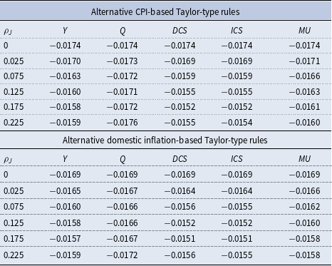
Note: DCS, ICS, and MU refer to domestic credit spread, international credit spread, and markup, respectively.

Figure 4 shows the welfare gains from credit policy according to the feedback parameters. Firstly, notice that the foreign financial shocks reduce the welfare by $1.6\%$ of steady state welfare per period without credit policy. While an increase in the feedback coefficient monotonically increase the welfare, a welfare gap between the coefficients with international credit spread and those with domestic credit spread broadens by $35\%$ from the initial welfare losses. Thus, this welfare analysis explicitly shows that credit policy based on international credit spread is superior to monetary policy and credit policy based on domestic credit spread. Notice that while moderate credit policy based on international credit spread (i.e., $\vartheta _{i}=20$ ) can eliminate welfare losses, aggressive credit policy based on domestic credit spread is required.

Figure 5. Impulse responses under alternative domestic inflation-based Taylor rules.

Note: DB and GB refer to domestic bank and global bank, respectively.

The central bank may not able to resort credit policy in the global financial crisis and thus, we evaluate various types of monetary policy rules associated with the welfare. Specifically, the different types of CPI-based and domestic inflation-based Taylor rules follow ¹⁷

(74) \begin{align} \hat {i}_{t}= \rho _{i}\hat {i}_{t-1} + (1 - \rho _{i})(\rho _{\pi }{\pi }_{t} + \rho _{J}\hat {J}_{t}); \;\ \hat {i}_{t}= \rho _{i}\hat {i}_{t-1} + (1 - \rho _{i})(\rho _{\pi }{\pi }_{h,t} + \rho _{J}\hat {J}_{t}) \end{align}

where $J\in \lbrace {Y},{Q},{DCS},{ICS},{MU}\rbrace$ . ¹⁸

Table 2 reports welfare losses in response to the shocks for the different types of the Taylor rules when $\vartheta =0$ and $\vartheta ^{f}=0$ . All entries are expressed as percentage units of steady state consumption. Under the Taylor coefficient of $\rho _{J}=0.175$ , the Taylor rules with domestic credit spread (DCS) and international credit spread (ICS) outperform the Taylor rules with output, real exchange rate and markup (MU) for both CPI-based and domestic inflation-based Taylor rules. In particular, credit spread based Taylor rules reduce the welfare losses by around $0.16\%$ per period, compared with the real exchange rate based Taylor rule. Thus, in the global financial crisis, credit spread based Taylor rules can be the best alternative policy by stabilizing fluctuations of asset prices along with domestic inflation volatility if the central bank is unable to resort credit policy while it still has a limited capacity to alleviate the crisis. As Figure 5 shows, under the domestic inflation-based Taylor rules with $\rho _{J}=0.175$ , the Taylor rules with international credit spread (ICS) further stabilizes output and domestic inflation, and thereby generating the lowest welfare losses.

Figure 6. Welfare analysis of credit policy.

Note: DCS, ICS and FI refer to domestic credit spread, international credit spread and international financial imperfections, respectively.

Figure 6 shows the welfare gains of credit policy according to the international financial imperfections, the degree of trade openness and the degree of banking system instability for sensitivity analysis. As for the international financial imperfections (i.e., $\chi \neq 0$ , $\Upsilon \neq 0$ ), while the imperfections cannot change effectiveness of credit policy based on domestic spread, the reverse is true for credit policy based on international spread. The higher levels of international financial imperfections, the lower global bank interest rate and thus, improves effectiveness of the latter under the aggressive international financial imperfections. Turning to $\Gamma$ and $\alpha$ , the international credit spread rule outperforms the domestic credit spread rule for all possible parameter values and thus, our results are invariant with respect to the parameter values given. Under the international credit spread rule, an increase (decrease) in $\Gamma$ ( $\alpha$ ) monotonically raises volatilities of the exchange rate and asset prices so that the economy with higher (lower) degree of banking system instability (trade openness) and the economy exposed to larger shocks benefits more from the rule.

5. Concluding remarks

In this paper, we have developed a small open economy DSGE model with a global banking system and global relative price adjustments with incomplete asset market to investigate the role of international financial imperfections. Then, we have assessed quantitatively how foreign shocks affect the small open economy, and evaluated the effects of credit policy based on domestic and international credit spread, and monetary policy.

We have found that among alternative monetary policy rules, the Taylor rule with international credit spread outperforms other types of alternative monetary policy rules, and that credit policy according to international credit spread outperforms credit policy according to domestic credit spread since the former attempts to remove distortions from international financial imperfections and reduces real costs of foreign loans. Thus, international financial imperfections play a major role in monetary and credit policies in an open economy.

In addition to investigate the role of international financial imperfections in monetary and credit policies, it would be interesting to investigate the role in the optimal monetary policy and macro-prudential policies. Due to multiple distortions from an imperfect risk sharing in consumption, and deviations from the uncovered interest parity for both international bond markets and global banking sectors, the optimal policy might attempt to achieve a second-best and allow some fluctuations in inflation and the output gap by targeting also on the distortions.