UNITARY REPRESENTATIONS OF CYCLOTOMIC HECKE ALGEBRAS AT ROOTS OF UNITY: COMBINATORIAL CLASSIFICATION AND BGG RESOLUTIONS

Abstract

We relate the classes of unitary and calibrated representations of cyclotomic Hecke algebras, and, in particular, we show that for the most important deformation parameters these two classes coincide. We classify these representations in terms of both multipartition combinatorics and as the points in the fundamental alcove under the action of an affine Weyl group. Finally, we cohomologically construct these modules via BGG resolutions.

Introduction

Unitary representations play a fundamental role in the representation theory of real, complex and p-adic reductive groups [4, 55, 23, 6]. Unitary representations are often the most important representations appearing ‘in nature’ via quantum mechanics [56] and harmonic analysis [42]. Furthermore, they tend to admit nice structural and homological properties, such as explicit eigenbases and resolutions by Verma modules.

In this paper, we study unitary representations of a family of infinite discrete groups: the affine braid groups. These are groups $B^{ea}_{n}$ of n braids on the cylinder (see [29]) and project onto the usual Artin braid groups by “flattening” the cylinder. Of course, the representation theory of the group $B^{ea}_{n}$ is extremely complicated and the problem would be intractable without imposing certain conditions on our representations. The condition we impose is that our representations factor through an affine Hecke quotient of the group algebra $\mathbb {C}B^{ea}$ , that is, the following skeinlike relation is satisfied

(†) $$ \begin{align} (T_{i} - q)(T_{i} + 1) = 0 \end{align} $$

for some $q \in \mathbb {C}^{\times }$ and every $i = 1, \dots , n-1$ , where $T_{i}$ is the overcrossing of the ith and $(i+1)$ -st strands. The algebra $\mathcal {H}^{\mathsf {aff}}_{q}(n) := \mathbb {C}B^{ea}_{n}/(T_{i} - q)(T_{i} + 1) $ is known as the affine Hecke algebra. Besides being interesting in and of itself, the algebra $\mathcal {H}^{\mathsf {aff}}_{q}(n)$ appears in the theory of knot invariants, categorification and the representation theory of p-adic reductive groups. Let us now discuss our methods and results in more detail.

First main result

First, we relate the unitary representations of $\mathcal {H}^{\mathsf {aff}}_{q}(n)$ to the class of calibrated representations. These are a well-studied class of representations of $\mathcal {H}^{\mathsf {aff}}_{q}(n)$ that are defined by the condition that the Jucys–Murphy subalgebra $\mathbb {A} \subseteq \mathcal {H}^{\mathsf {aff}}_{q}(n)$ acts semisimply; see [46, 45, 50, 40]. Calibrated representations exhibit many of the properties that make unitary representations interesting (for example, by definition they come equipped with an $\mathbb {A}$ -eigenbasis, which for simple calibrated representations is unique up to scalar multiplication), and it easily follows that, in fact, every unitary representation is calibrated. The converse is of course not true, but it turns out that if we restrict to certain representations (in a sense, the most complicated ones), then the story changes. To be more precise, every irreducible representation of $\mathcal {H}^{\mathsf {aff}}_{q}(n)$ factors through a cyclotomic quotient, $\mathcal {H}_{q, Q_1, \dots , Q_{\ell }}(n)$ which depends on several parameters $q, Q_1, \dots , Q_{\ell }$ . The representation theory of $\mathcal {H}_{q, Q_1, \dots , Q_{\ell }}(n)$ is most interesting when we specialise the parameter q to be a root of unity and the parameters $Q_i=q^{s_i} $ for $1\leq i \leq \ell $ .

Theorem A. Let $e \geq 2$ and $s_1, \dots , s_{\ell }$ be integers. Let $q = \exp (2\pi \sqrt {-1}/e)$ and $Q_{i} = q^{s_{i}}$ . A representation of the algebra $\mathcal {H}_{q, Q_1, \dots , Q_{\ell }}$ is unitary if and only if it is calibrated.

Second main result

Next, we use Theorem A to combinatorially classify the unitary representations. Given an integer $e> 1$ and $\mathbf {s} = (s_1, \dots , s_{\ell })\in \mathbb {Z}^{\ell }$ a charge, we denote the algebra $\mathcal {H}_{q, Q_1, \dots , Q_{\ell }}(n)$ as above simply by $\mathcal {H}_{\mathbf {s}}(n)$ . The definition of the algebra $\mathcal {H}_{\mathbf {s}}(n)$ depends only on the reduction modulo e of the charge $\mathbf {s}$ , so we can assume that $s_1\leq s_2\leq \ldots \leq s_{\ell }< s_1+e$ . Our choice of charge allows us to provide a particularly simple classification of unitary modules in terms of multipartition combinatorics.

Theorem B. Let $q = \exp (2\pi \sqrt {-1}/e)$ , and fix a charge $\mathbf {s}=(s_1,\dots s_{\ell })$ such that $s_1\leq s_2\leq \ldots \leq s_{\ell }< s_1+e$ . The simple $\mathcal {H}_q^{\mathrm {aff}}(n)$ -module $D_{\mathbf {s}}({\boldsymbol {\lambda }})$ is unitary if and only if the following equivalent conditions hold:

• • ${\boldsymbol {\lambda }}$ is cylindric, its right border strip has period at most e and its reading word is increasing;

• • ${\boldsymbol {\lambda }}\in \mathcal {F}_{\underline {h}} $ the fundamental alcove under an $\mathbf {s}$ -shifted action of an affine Weyl group of type A;

• • $D_{\mathbf {s}}({\boldsymbol {\lambda }})$ is calibrated.

Precise definitions for the terminology in the first two conditions are given in Sub sections 3.1 and 5.1.

Theorem B gives the first classification of calibrated representations for the algebra $\mathcal {H}_{ \mathbf {s}}(n)$ in terms of Young diagrams of multipartitions. Note that other combinatorial classifications in terms of weights and skew-Young diagrams are given in [45, 46]. Theorem B can be seen as the analogue of [37, Theorem 4.1] for calibrated representations—both results provide the first closed-form description of the given family of irreducible modules in terms of multipartitions.

Third main result

The combinatorial description of the unitary representations in Theorem B leads to our third main result, a multiplicity-free character formula for these representations and their cohomological construction by way of BGG, or Berstein-Gelfand-Gelfand, resolutions.

If we consider formal parameters $q, Q_1, Q_2, \dots , Q_{\ell }$ and define the algebra $\mathcal {H}_{q, Q_1, \dots , Q_{\ell }}(n)$ over the field of rational functions $\mathbb {C}(q, Q_1, \dots , Q_{\ell })$ , then the algebra $\mathcal {H}_{q, Q_1, \dots , Q_{\ell }}(n)$ is semisimple and the simple Specht modules $S(\boldsymbol {\mu })$ are indexed by the set of $\ell $ -multipartitions $\boldsymbol {\mu }$ of n, cf. [2, Proposition 3.10]. For $e> 1$ and $\mathbf {s}\in \mathbb Z^{\ell }$ , one can place a corresponding integral lattice on each Specht module $S(\boldsymbol {\mu })$ , obtaining a family of (nonsemisimple) $\mathcal {H}_{\mathbf {s}}(n)$ -modules $S_{\mathbf {s}}(\boldsymbol {\mu })$ by specialisation of the parameters $q = \exp (2\pi \sqrt {-1}/e)$ and $Q_{i} = q^{s_{i}}$ . Our choice of $\mathbf {s} \in {\mathbb {Z}}^{\ell }$ allows us to construct the unitary simple $D_{\mathbf {s}}({\boldsymbol {\lambda }})$ as the head of the Specht module $S_{\mathbf {s}}({\boldsymbol {\lambda }})$ for ${\boldsymbol {\lambda }}$ as in Theorem B. A BGG resolution of $D_{\mathbf {s}}({\boldsymbol {\lambda }})$ is a resolution of $D_{\mathbf {s}}({\boldsymbol {\lambda }})$ by a complex whose terms are direct sums of Specht modules $S_{\mathbf {s}}(\boldsymbol {\mu })$ .

Given a unitary simple module $D_{\mathbf {s}}({\boldsymbol {\lambda }})$ , we consider the set of multipartitions $\boldsymbol {\mu }$ dominating ${\boldsymbol {\lambda }}$ and having the same residue multiset as ${\boldsymbol {\lambda }}$ (with respect to the charge $\mathbf {s}$ ). For such $\boldsymbol {\mu }$ , we write $\boldsymbol {\mu }\trianglerighteq {\boldsymbol {\lambda }}$ ; see Section 1. The affine symmetric group $\widehat {\mathfrak {S}}_h$ , where h is the number of rows of ${\boldsymbol {\lambda }}$ , acts naturally on this set of multipartitions, endowing it with the structure of a graded poset in which ${\boldsymbol {\lambda }}$ is the unique element of length $0$ . We then construct a BGG resolution of $D_{\mathbf {s}}({\boldsymbol {\lambda }})$ as follows.

Theorem C. Associated to each unitary simple module, $D_{\mathbf {s}}({\boldsymbol {\lambda }})$ , we have a complex $ C_{\bullet } ({\boldsymbol {\lambda }})= \bigoplus _{ \begin {subarray}c \boldsymbol {\mu } \trianglerighteq {\boldsymbol {\lambda }} \end {subarray} }S_{\mathbf {s}}(\boldsymbol {\mu })\langle \ell (\boldsymbol {\mu })\rangle $ with differential given by an alternating sum over all “imple reflection homomorphisms’. This complex is exact except in degree zero, where $H_0(C_{\bullet }( {\boldsymbol {\lambda }} ))= D_{\mathbf {s}}({\boldsymbol {\lambda }}).$ The underlying graded character is as follows:

(††) $$ \begin{align} [D_{\mathbf{s}}({\boldsymbol{\lambda}})] = \sum_{ \begin{subarray}c \boldsymbol{\mu} \trianglerighteq {\boldsymbol{\lambda}} \end{subarray} } (-t)^{\ell(\boldsymbol{\mu})}[S_{\mathbf{s}}(\boldsymbol{\mu})\langle \ell(\boldsymbol{\mu})\rangle]. \end{align} $$

Moreover, the module $D_{\mathbf {s}}({\boldsymbol {\lambda }})$ admits a characteristic-free basis $\{c_{\mathsf {S}}\otimes _{\mathbb {Z}} \Bbbk \mid \mathsf {S}\in \mathrm {Path}_{ {{\underline {h}}}}^{\mathcal {F}}(\lambda ) \}$ where $ \mathrm {Path}_{ {{\underline {h}}}}^{\mathcal {F}}(\lambda )\subseteq \mathrm {Path}_{ {{\underline {h}}}} (\lambda )$ is the subset of paths which never leave the fundamental alcove $\mathcal {F}_{\underline {h}}$ .

In the case of the unitary representations of the Hecke algebra of the symmetric group, the resolutions of Theorem C were the subject of the authors’ previous work [13] and Theorem C reproves a conjecture of Berkesch–Griffeth–Sam [7]. Theorem C vastly generalises this work to all unitary representations of all cyclotomic Hecke algebras. We remark that we concentrate on the roots of unity case in this paper. When q is not a root of unity, unitary simple representations admit BGG resolutions, which were constructed by Cherednik in [19]. Our results and those of [17, 18, 31] intersect in a few special cases.

Aspects of this story should be very familiar to the experts: We have an algebraic object (in this case a cyclotomic or affine Hecke algebra) for which there exists a ‘nice family’ of irreducible representations (in this case, the unitary representations) which can be combinatorially classified and constructed via explicit bases and BGG resolutions. Analogous stories exist for ladder representations of p-adic groups [5], finite-dimensional representations of (Kac–Moody) Lie algebras [8, 38] and homogeneous representations of antispherical Hecke categories [12].

We remark that, while the definition of a unitary module depends crucially on the ground field being $\mathbb C$ , the condition to be calibrated makes sense for arbitrary fields. In this manner, Theorems B and C both admit characteristic-free generalisations which are proven in this paper.

Regular p -Kazhdan–Lusztig theory. The coefficients in equation (††) are equal to ‘regular’ (or ‘nonsingular’) inverse (p-)Kazhdan–Lusztig polynomials. In fact, the proof of Theorem B involves passing from the cyclotomic Hecke algebras to the setting of Elias–Williamson’s diagrammatic category for ‘regular’ Soergel-bimodules. For the general linear group, $\mathrm {GL}_h$ , the ‘regular’ Soergel-bimodules control the representation theory of the principal block (the block containing the trivial representation $\Bbbk =\Delta (k^h)$ for $n=kh$ ) if and only if $p> h$ . On the other side of Schur–Weyl duality, this means that ‘regular’ Soergel-bimodules control the representation theory of the Serre subcategory of $\Bbbk \mathfrak {S}_n$ - $\mathrm {mod} $ corresponding to the poset $\{\lambda \mid \lambda \trianglerighteq (k^h) \text { for }n=kh\}$ , and we remark that the simple $\Bbbk \mathfrak {S}_n$ -module labelled by the partition $ (k^h)$ is calibrated providing $p>h$ .

For higher levels $\ell>1$ , one can ask ‘to what extent is the cyclotomic Hecke algebra controlled by regular (p-)Kazhdan–Lusztig theory?’ Of course, the Schur–Weyl duality with the general linear group no longer exists. However, one can speak of calibrated representations of the cyclotomic Hecke algebra. In fact, the largest Serre subcategory of (a block of) the cyclotomic Hecke algebra controlled by regular p-Kazhdan–Lusztig theory is given by the poset $\{\boldsymbol {\mu } \mid \boldsymbol {\mu } \trianglerighteq {\boldsymbol {\lambda }}\}$ , where $D_{\mathbf {s}}({\boldsymbol {\lambda }} )$ is the minimal calibrated simple module in the block (under the order $ \trianglerighteq $ ). Thus, the Serre quotients carved out by calibrated representations of cyclotomic Hecke algebras play the same role as that of principal blocks of algebraic groups for $p>h$ .

Structure of the paper. Section 1 introduces the combinatorics that will play an important role in this paper. Then we study unitary representations in Section 2 where we prove Theorem A; see Theorem 2.21. Sections 3 and 4 are devoted to the proof of Theorem B, which involves intricate combinatorial constructions. In Section 5, we recall previous work of the first author together with A. Cox and A. Hazi [10] that will allow us to prove Theorem C. We do this in Section 6. In this section, we also discuss the consequences of our work in the representation theory of rational Cherednik algebras; see Remark 6.31. Finally, in Appendix A, we use our techniques to give a complete classification of unitary representations of the Hecke algebra of the symmetric group. While this has mostly appeared in the literature, see [52]. We believe it gives a good feeling for the usage of calibrated representations in this setting and corrects an oversight of [52].

1 Combinatorics

1.1 Charges, multipartitions and tableaux

Fix $e\in \mathbb {Z}_{\geq 2}$ throughout this paper.

Definition 1.1. We call an $\ell $ -tuple of integers $\mathbf {s}=(s_1,s_2,\ldots , s_{\ell })\in \mathbb {Z}^{\ell }$ an $\ell $ -charge or simply a charge. Given $e\in \mathbb {Z}_{\geq 2}$ , we say that $\mathbf {s}$ is cylindrical if $s_1\leq s_2\leq \ldots \leq s_{\ell }< s_1+e$ .

We define a composition $\lambda $ of n to be a finite sequence of nonnegative integers $ (\lambda _1,\lambda _2, \ldots )$ whose sum $|\lambda | = \lambda _1+\lambda _2 + \dots $ equals n. We say that $\lambda $ is a partition if, in addition, this sequence is weakly decreasing. We let $\lambda ^t$ denote the transpose partition. An $\ell $ -multicomposition (respectively $\ell $ -multipartition or simply $\ell $ -partition) ${\boldsymbol {\lambda }}=(\lambda ^1,\lambda ^2,\ldots ,\lambda ^{\ell })$ of n is an $\ell $ -tuple of compositions (respectively partitions) such that $|{\boldsymbol {\lambda }}| := |\lambda ^1|+|\lambda ^2|+\ldots + |\lambda ^{\ell }|=n$ . We will denote the set of $\ell $ -multicompositions (respectively $\ell $ -partitions) of n by $\mathscr {C}_{\ell }(n)$ (respectively by $\mathscr {P}_{\ell }(n)$ ). Given ${\boldsymbol {\lambda }}=(\lambda ^1,\lambda ^2,\ldots ,\lambda ^{\ell }) \in \mathscr {P}_{\ell }(n)$ , the Young diagram of ${\boldsymbol {\lambda }}$ is defined to be the set of boxes (or nodes),

$$\begin{align*}\{(r,c,m) \mid 1\leq c\leq \lambda^m_r,\;1 \leq m \leq \ell \}. \end{align*}$$

We do not distinguish between the multipartition and its Young diagram. We draw the Young diagram of a partition by letting c increase from left to right and r increase from top to bottom. We refer to a box $(r,c,m)$ as being in the rth row and cth column of the mth component of ${\boldsymbol {\lambda }}$ . We draw the Young diagram of a multipartition by placing the Young diagrams of $\lambda ^1,\ldots ,\lambda ^{\ell }$ side by side from left to right as m runs from $1$ to $\ell $ . Finally, a tableau $\mathsf {T}$ on a multipartition ${\boldsymbol {\lambda }}$ is a bijection from the set of boxes of ${\boldsymbol {\lambda }}$ to $\{1, 2, \dots , |{\boldsymbol {\lambda }}|\}$ . The tableau $\mathsf {T}$ is called standard if it is increasing along the rows and columns of each component. We let $\mathrm { Std}({\boldsymbol {\lambda }})$ denote the set of all standard tableaux on ${\boldsymbol {\lambda }}$ . If $\mathsf {T} \in \mathrm { Std}({\boldsymbol {\lambda }})$ is a standard tableau, then $\operatorname {Shape}(\mathsf {T}{\downarrow }_{\{1,\dots ,k\}})$ is the multipartition whose Young diagram consists of all the boxes with labels $\leq k$ . Finally, we denote by $\varnothing $ the empty multipartition.

Example 1.2. Let $\ell =3$ and ${\boldsymbol {\lambda }}=(\lambda ^1,\lambda ^2,\lambda ^3)=((2,1),(4,2,1),(5))$ . We draw the Young diagram of ${\boldsymbol {\lambda }}$ as follows:

Definition 1.3. A charged $\ell $ -partition is the data of an $\ell $ -partition ${\boldsymbol {\lambda }}$ together with an $\ell $ -charge $\mathbf {s}\in {\mathbb {Z}}^{\ell }$ . Given a box $b=(r,c,m)\in {\boldsymbol {\lambda }}$ , we define its charged content to be $\mathsf {co}^{\mathbf {s}}(b) = s_m+ c - r$ and we define its residue to be $\mathsf {res}^{\mathbf {s}}(b) := \mathsf {co}^{\mathbf {s}}(b) \pmod e$ . We refer to a box of residue $i\in {\mathbb {Z}}/e{\mathbb {Z}}$ as an i-box (or i-node).

Note that the residue of a box in ${\boldsymbol {\lambda }}$ depends on the choice of the charge $\mathbf {s}\in \mathbb Z^{\ell }$ . For a tableau $\mathsf {T}$ on ${\boldsymbol {\lambda }}$ , we let ${\mathrm {res} (\mathsf {T})}$ denote the residue sequence consisting of $\mathrm {res} (\mathsf {T}^{-1}(k))$ for $k=1,\dots , n$ in order.

Example 1.4. Let $\ell =3$ and ${\boldsymbol {\lambda }}=(\lambda ^1,\lambda ^2,\lambda ^3)=((2,1),(4,2,1),(5))$ . Let $\mathbf {s}=(-1,2,0)\in \mathbb {Z}^3$ . The Young diagram of ${\boldsymbol {\lambda }}$ with its boxes labelled by their charged contents looks as follows:

Now, take $e=4$ , then labelling the boxes of the Young diagram of ${\boldsymbol {\lambda }}$ their residues, we have:

and we have that $ \mathrm {res}(\mathsf {T}_{{\boldsymbol {\lambda }}})= (0,2,1,0,3,2,1,3,2,0,2,0,3,1,0) \in ( \mathbb Z / e \mathbb Z)^{15},$ where $\mathsf {T}_{{\boldsymbol {\lambda }}}$ is the reverse column-reading tableau on ${\boldsymbol {\lambda }}$ ; see Example 1.10 below.

Definition 1.5. Given $\mathbf {s}\in \mathbb {Z}^{\ell }$ and two i-boxes $(r,c,m), (r',c',m')\in {\boldsymbol {\lambda }}$ for some $i\in {\mathbb {Z}}/e{\mathbb {Z}}$ , we write $(r,c,m)\rhd _{\mathbf {s}} (r',c',m')$ if $\mathsf {co}^{\mathbf {s}}(r,c,m)> \mathsf {co}^{\mathbf {s}}(r',c',m')$ or $\mathsf {co}^{\mathbf {s}}(r,c,m) = \mathsf {co}^{\mathbf {s}}(r',c',m')$ and $m<m'$ . For ${\boldsymbol {\lambda }},\boldsymbol {\mu }\in \mathscr {P}_{ \ell } (n)$ , we write $ \boldsymbol {\mu } \trianglelefteq {\boldsymbol {\lambda }} $ if there is a residue preserving bijective map $\mathsf {A}:[{\boldsymbol {\lambda }}] \to [\boldsymbol {\mu }]$ such that either $ \mathsf {A}(r,c,m)\vartriangleleft _{\mathbf {s}} (r,c,m) $ or $ \mathsf {A}(r,c,m)=(r,c,m) $ for all $(r,c,m)\in {\boldsymbol {\lambda }}$ . When $\mathbf {s}\in \mathbb {Z}^{\ell }$ is cylindrical, we often write $\rhd $ instead of $\rhd _{\mathbf {s}}$ .

Remark 1.6. The ordering of Definition 1.5 is one of many possible cellular orderings on the Hecke algebra. It is important (and useful for this paper) because it is the only ordering for which we have a closed combinatorial description of the indexing set of simple modules; see [27, 9] for more details.

Definition 1.7. Given a partition $\lambda =(\lambda _1,\dots ,\lambda _h)$ such that $\lambda _h>0$ , we set $h(\lambda )$ to be the height of the partition, that is $h(\lambda )=h$ . Given a multipartition ${\boldsymbol {\lambda }}=(\lambda ^1,\lambda ^2,\dots , \lambda ^{\ell })$ , we set $h({\boldsymbol {\lambda }})=(h_1,\dots ,h_{\ell })$ to be the $\ell $ -composition formed of the heights of the component partitions. Given ${\boldsymbol {\lambda }}=(\lambda ^1,\lambda ^2,\dots , \lambda ^{\ell })$ , we define the height of the multipartition to be the integer $h_{{\boldsymbol {\lambda }}}=h_1+\dots +h_{\ell }$ .

Definition 1.8. Fix ${\mathbf {s} } \in {\mathbb {Z}}^{\ell }$ . We say that a composition $\underline { h }= ( h _1,\dots , h _{\ell }) $ of h is ${\mathbf {s} }$ -admissible if $ h _m\leq s_{m}-s_{m-1 } $ for $1< m \leq \ell $ and $ h _1\leq e+s_1-s_{\ell } $ and with at least one of these inequalities being strict. We refer to any value $1\leq m\leq \ell $ for which the inequality is strict as a step change. For an $\mathbf {s}$ -admissible $\underline { h }\in \mathbb N^{\ell }$ , we let $\mathscr {P}_{\underline {h}} (n)$ denote the set of all ${\boldsymbol {\lambda }}\in \mathscr {P}_{\ell } (n)$ such that $h({\boldsymbol {\lambda }})=\underline { h }$ .

Definition 1.9. Let ${\underline {h}}\in \mathbb {N}^{\ell }$ be $\mathbf {s}$ -admissible, and let $1\leq m \leq \ell $ . Given ${\boldsymbol {\lambda }} \in \mathscr {P}_{{\underline {h}}}(n)$ , we define the reverse column reading tableau, $\mathsf {T}_{(m,{\boldsymbol {\lambda }})}$ , to be the standard tableau obtained by filling the first column of the $(m-1)$ th component then the first column of the $(m-2)$ th component and so on until finally filling the first column of the mth component and then repeating this procedure on the second columns, the third columns, and so on. Here, we take the ‘cyclic’ convention that the $(m-1)$ th component for $m=1$ is simply the $\ell $ th component.

Example 1.10. Definition 1.9 is best illustrated via an example. Let $\mathbf {s} =(0,3,4 )$ with $e=7$ . We have that $\lambda =((2,1),(4,2,1),(5))\in \mathscr {P}_{(2,3,1)}(15)$ and that $h_1=2<7+0-4=e+s_1-s_{\ell }$ and so $m=1$ is a step change (one can check that this step change is unique). The reverse reading column reading tableau $\mathsf {T}_{1,{\boldsymbol {\lambda }}}$ is given by filling the first columns of the third component, second component, first component and then the second columns of these components…hence obtaining

Given ${\boldsymbol {\lambda }} \in \mathscr {P}_{\underline {h}}(n)$ , we let $\mathrm {Add}_{\underline {h}}({\boldsymbol {\lambda }})$ (respectively $\mathrm {Rem}_{\underline {h}}({\boldsymbol {\lambda }})$ ) denote the set of all addable (respectively removable) boxes of the Young diagram so that the resulting Young diagram is the Young diagram of a multipartition belonging to $\mathscr {P}_{\underline {h}}(n+1)$ (respectively $\mathscr {P}_{\underline {h}}(n-1)$ ). We let $\mathrm {Add}^i_{\underline {h}}({\boldsymbol {\lambda }})$ (respectively $\mathrm {Rem}^i_{\underline {h}}({\boldsymbol {\lambda }})$ ) denote the subset of nodes of residue equal to $i\in {\mathbb {Z}}/e{\mathbb {Z}}$ . Dropping the subscript ${\underline {h}}$ , we obtain the usual sets of addable and removable i-nodes of a multipartition.

Definition 1.11. Given $1\leq k\leq n$ and a standard tableau $\mathsf {T}$ on a multipartition ${\boldsymbol {\lambda }}$ , we let ${\mathcal A} _{\mathsf {T}}(k)$ (respectively ${\mathcal R} _{\mathsf {T}}(k)$ ) denote the set of all addable $\mathrm {res} (\mathsf {T}^{-1}(k))$ -boxes (respectively all removable $\mathrm {res} (\mathsf {T}^{-1}(k))$ -boxes) of the multipartition $\operatorname {Shape}(\mathsf {T}{\downarrow }_{\{1,\dots ,k\}})$ which are more dominant than $\mathsf {T}^{-1}(k)$ . We define the degree of $\mathsf {T}\in \mathrm {Std}({\boldsymbol {\lambda }})$ for ${\boldsymbol {\lambda }} \in \mathscr {P} (n)$ as follows:

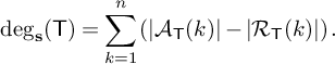$$ \begin{align*} \deg_{\mathbf{s} } (\mathsf{T}) = \sum_{k=1}^n \left( |{\mathcal A} _{\mathsf{T}}(k)|-|{\mathcal R} _{\mathsf{T}}(k)| \right). \end{align*} $$

Remark 1.12. Let ${\underline {h}} \in \mathbb N^{\ell }$ be ${\mathbf {s} }$ -admissible and $1\leq m \leq \ell $ be a step change. We have that $\deg _{\mathbf {s} } (\mathsf {T}_{(m,{\boldsymbol {\lambda }})})=0$ for ${\boldsymbol {\lambda }} \in \mathscr {P}_{ {\underline {h}}}(n)$ .

1.2 The $\widehat {\mathfrak {sl}}_e$ -crystal

Ariki proved that the $\widehat {\mathfrak {sl}}_e$ -crystal explicitly realises the modular branching rule of the cyclotomic Hecke algebra [3]. We now recall the combinatorics of this construction. Fix $e\geq 2$ and a charge $\mathbf {s} \in \mathbb {Z}^{\ell }$ . The $\widehat {\mathfrak {sl}}_e$ -crystal is a simply directed graph on the set of vertices consisting of all $\ell $ -partitions. Its arrows are given by a rule for adding at most one box of each residue $i\in \mathbb {Z}/e\mathbb {Z}$ to a given $\ell $ -partition. We define the crystal operators $\tilde {e}_i$ and $\tilde {f}_i$ , which remove and add (respectively) at most one box of residue i.

Definition 1.13 [27, Theorem 2.8]

Fix $i\in \mathbb {Z}/e\mathbb {Z}$ , $\mathbf {s}\in \mathbb {Z}^{\ell }$ and an $\ell $ -partition ${\boldsymbol {\lambda }}$ .

• • Form the i-word of ${\boldsymbol {\lambda }}$ by listing all addable and removable i-boxes of ${\boldsymbol {\lambda }}$ in increasing order from left to right (according to $\rhd _{\mathbf {s}}$ ) and then replacing each addable box in the list by the symbol $+$ and each removable box by the symbol $-$ .

• • Next, find the reduced i-word of ${\boldsymbol {\lambda }}$ by recursively canceling all adjacent pairs $(-+)$ in the i-word of ${\boldsymbol {\lambda }}$ . The reduced i-word is of the form $(+)^a(-)^b$ for some $a,b\in \mathbb {Z}_{\geq 0}$ .

• • Define $\tilde {f}_i$ as the operator that adds the addable i-box to ${\boldsymbol {\lambda }}$ corresponding to the rightmost $+$ in the reduced i-word of ${\boldsymbol {\lambda }}$ . If the reduced i-word of ${\boldsymbol {\lambda }}$ contains no $+$ , then we declare that $\tilde {f}_i{\boldsymbol {\lambda }}=0$ . Likewise, define $\tilde {e}_i$ as the operator that removes the removable i-box from ${\boldsymbol {\lambda }} $ corresponding to the leftmost $-$ in the reduced i-word of ${\boldsymbol {\lambda }}$ . If the reduced i-word of ${\boldsymbol {\lambda }}$ contains no $-$ , then we declare that $\tilde {e}_i{\boldsymbol {\lambda }}=0$ .

The directed graph with vertices all $\ell $ -partitions and arrows ${\boldsymbol {\lambda }}\stackrel {i}{\rightarrow }\boldsymbol {\mu }$ if and only if $\boldsymbol {\mu }=\tilde {f}_i{\boldsymbol {\lambda }}$ , $i\in \mathbb {Z}/e\mathbb {Z}$ , is called the $\widehat {\mathfrak {sl}}_e$ -crystal. We have $\tilde {f}_i\boldsymbol {\mu }={\boldsymbol {\lambda }}$ if and only if $\tilde {e}_i{\boldsymbol {\lambda }}=\boldsymbol {\mu }$ .

Definition 1.14. The i-box that is added by $\tilde {f}_{i}$ , if it exists, is called a good addable i-box of ${\boldsymbol {\lambda }}$ . Similarly, the box that is removed by $\tilde {e}_{i}$ is called a good removable i-box of ${\boldsymbol {\lambda }}$ .

Remark 1.15. Given $i\in \mathbb {Z}/e\mathbb {Z}$ , if ${\boldsymbol {\lambda }}$ has only one removable i-box b and no addable i-box of charged content greater than or equal to $\mathsf {co}^{\mathbf {s}}(b)$ , then $\tilde {e}_i({\boldsymbol {\lambda }})={\boldsymbol {\lambda }}\setminus \{b\}$ . We will use this observation without further mention.

The $\widehat {\mathfrak {sl}}_e$ -crystal is in general disconnected, and we will be interested in its connected component containing the empty multipartition $\varnothing $ . The vertices in this connected component of the $\widehat {\mathfrak {sl}}_e$ -crystal do not, in general, admit closed formulas (one must instead search for a sequence of good nodes by repeated use of Definition 1.13). However, for our choice of cylindric charge $\mathbf {s} \in {\mathbb {Z}}^{\ell }$ (as in Definition 1.1), we have the following combinatorial description from [27].

Definition 1.16. An $\ell $ -partition ${\boldsymbol {\lambda }}$ with charge $\mathbf {s}\in \mathbb {Z}^{\ell }$ is named FLOTW, after Foda, Leclerc, Okado, Thibon and Welsh, if the following conditions hold:

1. (1) The charge $\mathbf {s}$ is cylindrical,

2. (2) The multipartition ${\boldsymbol {\lambda }}$ is cylindrical, that is:

   1. (a) $\lambda ^j_k\geq \lambda ^{j+1}_{k+s_{j+1}-s_j}$ for all $j\in \{1,\ldots , \ell -1\}$ and for all $k\geq 1$ ,

   2. (b) $\lambda ^{\ell }_k\geq \lambda ^1_{k+e+s_1-s_{\ell }}$ for all $k\geq 1$ ,

3. (3) For all $\alpha>0$ , the residues modulo e of the rightmost boxes of the rows of size $\alpha $ do not cover $\{0,\ldots ,e-1\}$ .

2 Unitary representations

2.1 The affine Hecke algebra

Let us recall that the (extended) affine braid group, $B^{ea}_{n}$ has generators $T_{1}, \dots , T_{n-1}, x_{1}, \dots , x_{n}$ subject to the following relations:

1. (a) $T_{i}T_{i+1}T_{i} = T_{i+1}T_{i}T_{i+1}$ and $T_{i}T_{j} = T_{j}T_{i}$ if $|i - j|> 1$ .

2. (b) $x_{i}x_{j} = x_{j}x_{i}$ for every $i, j = 1, \dots , n$ .

3. (c) $T_{i}x_{i}T_{i} = x_{i+1}$ , $T_{i}x_{j} = x_{j}T_{i}$ if $j \neq i, i+1$ .

We may think of $B^{ea}_{n}$ as the braid group on the cylinder. The element $T_{i}$ corresponds to the usual braid generator that crosses two adjacent strands, and the element $x_{i}$ corresponds to looping the ith strand around the cylinder so that it comes back to the ith position; see Figure 1 below.

Figure 1 The braid generators $x_{i}$ and $T_{i}$ . We remark that these are braids on a cylinder, so the left and right sides of the rectangles are to be identified.

The affine Hecke algebra is the quotient of the group algebra of $B^{ea}_{n}$ by a skein-type relation.

Definition 2.1. Let $\mathsf {R}$ be a domain and $q \in \mathsf {R}^{\times }$ , $q \neq \pm 1$ . The (extended) affine Hecke algebra $\mathcal {H}^{\mathsf {aff}}_{q}(n, \mathsf {R})$ is the quotient of the group algebra $\mathsf {R}B^{ea}_{n}$ by the relations

$$ \begin{align*}(T_{i} + 1)(T_{i} - q) = 0 \end{align*} $$

for $i = 1, \dots , n-1$ . When the domain $\mathsf {R}$ is clear from the outset, we will simply denote the affine Hecke algebra by $\mathcal {H}^{\mathsf {aff}}_{q}(n)$ .

Remark 2.2. It is customary to define the elements $X_{i} := q^{1-i}x_{i}$ so that in $\mathcal {H}^{\mathsf {aff}}_{q}(n)$ we have the relation $T_{i}X_{i}T_{i} = qX_{i+1}$ .

Remark 2.3. The finite Hecke algebra $H_{q}(n)$ can be realized as a subalgebra of $\mathcal {H}^{\mathsf {aff}}_{q}(n)$ generated by $T_{1}, \dots , T_{n-1}$ . It can also be realized as the quotient $\mathcal {H}^{\mathsf {aff}}_{q}(n)/(X_1 - 1)$ . This is akin to the finite braid group $B_{n}$ being both a subgroup and a quotient group of $B^{ea}_{n}$ .

Remark 2.4. We remark that we are working with the so-called Bernstein presentation of the affine Hecke algebra; see, for example, [20, Chapter 7]. We will refer to $X_{1}, \dots , X_{n}$ as the Jucys–Murphy elements of $\mathcal {H}^{\mathsf {aff}}_{q}(n)$ ¹ . Accordingly, we will call the algebra $\mathbb {A} := \mathsf {R}[X_{1}^{\pm 1}, \dots , X_{n}^{\pm 1}] \subseteq \mathcal {H}^{\mathsf {aff}}_{q}(n)$ the Jucys–Murphy subalgebra. It is isomorphic to the algebra of Laurent polynomials in n variables, and we have a vector space decomposition $\mathcal {H}^{\mathsf {aff}}_{q}(n) = H_{q}(n) \otimes _{\mathsf {R}} \mathbb {A}$ .

When $\mathsf {R}$ is a domain of characteristic zero it is known (see, for example, [20, Proposition 7.1.14]) that the center of $\mathcal {H}^{\mathsf {aff}}_{q}(n)$ is $Z(\mathcal {H}^{\mathsf {aff}}_{q}(n)) = \mathbb {A}^{S_{n}}$ , the algebra of symmetric Laurent polynomials in the Jucys–Murphy elements. Thus, $\mathcal {H}^{\mathsf {aff}}_{q}(n)$ is finite over its center, and, when $\mathsf {R}$ is a field $\mathsf {F}$ of characteristic zero, every irreducible representation of $\mathcal {H}^{\mathsf {aff}}_{q}(n)$ is finite-dimensional. If moreover $\mathsf {F}$ is algebraically closed it follows, looking at the eigenvalues of $X_{1}$ , that every irreducible representation of $\mathcal {H}^{\mathsf {aff}}_{q}(n)$ factors through an algebra of the form

$$ \begin{align*}\mathcal{H}_{q, Q_1, \dots, Q_{\ell}}(n) := \frac{\mathcal{H}^{\mathsf{aff}}_{q}(n)}{\left(\prod_{i}^{\ell}(X_{1} - Q_{i})\right).} \end{align*} $$

This is known as the cyclotomic Hecke algebra, or the Ariki–Koike algebra. It is a finite-dimensional $\mathsf {F}$ -algebra, of dimension precisely $n!\ell ^{n}$ , [1].

2.2 Unitary representations

For this subsection, we let $\mathsf {R} = \mathbb {C}$ , the complex field. We make the convention that a Hermitian form on a finite-dimensional complex vector space is linear on the first variable and conjugate-linear on the second. Recall that we have defined the affine Hecke algebra $\mathcal {H}^{\mathsf {aff}}_{q}(n)$ as a quotient of the group algebra $\mathbb {C}B^{ea}_{n}$ , so the following notion makes sense.

Definition 2.5. We say that a finite-dimensional $\mathcal {H}^{\mathsf {aff}}_{q}(n)$ -representation is unitary if it admits a positive-definite $B^{ea}_{n}$ -invariant Hermitian form.

Note that all affine Hecke algebras admit a one-dimensional unitary representation, where all elements $T_{i}$ act by $-1$ . However, unless q is a root of unity this may be the only unitary representation, as the following result shows.

Lemma 2.6. Assume that $\mathcal {H}^{\mathsf {aff}}_{q}(n)$ admits a unitary representation M, such that there exist $i = 1, \dots , n-1$ and $m \in M$ with $T_{i}m = qm$ . Then, $q \in \mathbb {C}^{\times }$ lies in the unit circle.

Proof. Let $m \in M$ and i be as in the statement of the lemma. Then,

$$ \begin{align*}0 \neq q\langle m, m \rangle = \langle T_{i}m, m \rangle = \langle m, T_{i}^{-1}m\rangle = \overline{q^{-1}}\langle m, m\rangle \end{align*} $$

so that $q = \overline {q^{-1}}$ . Thus, q is in the unit circle.

Remark 2.7. We remark that Lemma 2.6 follows from the following more general result. Let G be any group, and let M be a finite-dimensional unitary representation of G. Then, every eigenvalue of g on M lies in the unit circle, for any $g \in G$ . Note that this statement is obvious when G is a finite group as in this case every eigenvalue of g is, in fact, a root of unity. The proof in the general case is just as that of Lemma 2.6.

Since every cyclotomic Hecke algebra $\mathcal {H}_{q, Q_1, \dots , Q_{\ell }}(n)$ is a quotient of the affine Hecke algebra, it makes sense to speak about unitary representations of $\mathcal {H}_{q, Q_1, \dots , Q_{\ell }}(n)$ . Just as in Lemma 2.6, we have that if $\mathcal {H}_{q, Q_1, \dots , Q_{\ell }}(n)$ admits a unitary representation, then all complex numbers $q, Q_1, \dots , Q_{\ell } \in \mathbb {C}^{\times }$ must lie in the unit circle.

Let us remark that the cyclotomic Hecke algebra $\mathcal {H}_{q, Q_1, \dots , Q_{\ell }}(n)$ is a quotient of the group algebra of a different braid group: the braid group $B(\ell , 1, n)$ , which is defined as follows. Let $G(\ell , 1, n) := S_{n} \ltimes (\mathbb {Z}/\ell \mathbb {Z})^{n}$ be the cyclotomic group. If we think of this group as the group of $n \times n$ permutation matrices whose nonzero entries are $\ell $ -roots of unity, we get an action of $G(\ell , 1, n)$ on $\mathfrak {h} := \mathbb {C}^{n}$ . Let $\mathfrak {h}^{reg}$ be the locus where this action is free. It can be shown that this is the complement of a hyperplane arrangement in $\mathbb {C}^n$ . Then,

$$ \begin{align*} B(\ell, 1, n) := \pi_{1}(\mathfrak{h}^{reg}/G(\ell, 1, n)). \end{align*} $$

For example, when $\ell = 1$ , the group $B(1, 1, n)$ is the usual Artin braid group on n strands. It is clear from the definitions (see, e.g., [16]) that a $\mathcal {H}_{q, Q_1, \dots , Q_{\ell }}(n)$ -representation is unitary if and only if it admits a positive-definite $B(\ell , 1, n)$ -invariant Hermitian form. On the other hand, Rouquier has shown using the representation theory of rational Cherednik algebras, [51, Proposition 4.5.4], that every irreducible $\mathcal {H}_{q, Q_1, \dots , Q_{\ell }}(n)$ -representation admits a (unique up to $\mathbb {R}^{\times }$ -scalars) nondegenerate $B(\ell , 1, n)$ -invariant Hermitian form. Thus, the question of unitarity is that of positive-definiteness of this form.

2.3 Unitary representations via $*$ -operations

In [6], Barbasch and Ciubotaru define a class of representations that are closely related to the unitary representations we study in this paper. The goal of this section is to explore this relation. In order to do so, throughout this subsection $\mathsf {R} = \mathbb {C}[\mathsf {q}, \mathsf {q}^{-1}]$ and $\mathcal {H}^{\mathsf {aff}}_{\mathsf {q}}(n) := \mathcal {H}^{\mathsf {aff}}_{\mathsf {q}}(n, \mathsf {R})$ .

Definition 2.8. A $*$ -operation on $\mathcal {H}^{\mathsf {aff}}_{\mathsf {q}}(n)$ is a conjugate-linear, involutive antiautomorphism of $\mathcal {H}^{\mathsf {aff}}_{\mathsf {q}}(n)$ . Given a $*$ -operation on $\mathcal {H}^{\mathsf {aff}}_{\mathsf {q}}(n)$ , a representation M of $\mathcal {H}^{\mathsf {aff}}_{\mathsf {q}}(n)$ is called $*$ -unitary if it admits a positive-definite Hermitian form which is $\mathcal {H}^{\mathsf {aff}}_{\mathsf {q}}(n)$ -invariant in the sense that

$$ \begin{align*}\langle am, m'\rangle = \langle m, a^{*}m'\rangle \end{align*} $$

for every $m, m' \in M$ , $a \in \mathcal {H}^{\mathsf {aff}}_{\mathsf {q}}(n)$ .

In [6], the authors define $*$ -operations on $\mathcal {H}^{\mathsf {aff}}_{\mathsf {q}}(n)$ and study the notion of unitary representations for these $*$ -operations. These are the first two $*$ -operations of the following proposition.

Proposition 2.9. The following formulas define $*$ -operations on $\mathcal {H}^{\mathsf {aff}}_{\mathsf {q}}(n)$ .

1. (1) $T_{i}^{\bullet } = T_{i}$ , $X_{i}^{\bullet } = X_{i}$ , $\mathsf {q}^{\bullet } = \mathsf {q}$ .

2. (2) $T_{i}^{\star } = T_{i}$ , $X_{i}^{\star } = T_{w_{0}}X^{-1}_{n-i+1}T_{w_{0}}^{-1}$ , $\mathsf {q}^{\star } = \mathsf {q}$ , where $T_{w_{0}} = T_{1}T_{2}\cdots T_{n-1}T_{1}T_{2}\cdots T_{n-2}\cdots T_{1}T_{2}T_{1}$ .

3. (3) $T_{i}^{\dagger } = T_{i}^{-1}$ , $X_{i}^{\dagger } = X_{i}^{-1}$ , $\mathsf {q}^{\dagger } = \mathsf {q}^{-1}$ .

Proof. For $\bullet $ and $\star $ , see [6, Definition 2.3.1]. For $\dagger $ , note that the relation $(T_{i}+1)(T_{i}-\mathsf {q}) = 0$ is equivalent to $(T_{i}^{-1} + 1)(T_{i}^{-1} - \mathsf {q}^{-1}) = 0$ , so this is preserved under $\dagger $ . It is also clear that $\dagger $ preserves the relations among the $X_{i}$ , as well as the braid relations among the $T_{i}$ . Finally, we have

$$ \begin{align*}(T_{i}X_{i}T_{i})^{\dagger} = T_{i}^{\dagger}X_{i}^{\dagger}T_{i}^{\dagger} = T_{i}^{-1}X_{i}^{-1}T_{i}^{-1} = (T_{i}X_{i}T_{i})^{-1} = \mathsf{q}^{-1}X_{i+1}^{-1} = (\mathsf{q} X_{i+1})^{\dagger} \end{align*} $$

which finishes the proof.

Remark 2.10. In [6, Definition 2.4.1], the authors term an $*$ -operation admissible if $\mathsf {q}^{*} = \mathsf {q}$ and $T_{i}^{*} = T_{i}$ for $i = 1, \dots , n-1$ . So the $*$ -operations $\bullet $ and $\star $ of Proposition 2.9 are admissible, while $\dagger $ is not. It is conjectured, [6, Conjecture 2.4.2] that $\bullet $ and $\star $ are essentially the only admissible $*$ -operations on $\mathcal {H}^{\mathsf {aff}}_{\mathsf {q}}(n)$ .

It is clear that a representation M of $\mathcal {H}^{\mathsf {aff}}_{\mathsf {q}}(n)$ is unitary in the sense of Definition 2.5 if and only if it is $\dagger $ -unitary in the sense of [6]. Representations that are $\star $ -unitary and $\bullet $ -unitary have been studied in loc. cit., where they are shown to be related to unitary representations of general linear groups over p-adic fields. Note that both $\bullet $ and $\star $ commute with the action of $\mathsf {q}$ , while $\dagger $ does not. Nevertheless, the $*$ -operations $\bullet $ and $\dagger $ are closely related, as witnessed by the following result.

Proposition 2.11. The map $\iota $ defined on generators by $\iota (T_{i}) = T_{i}^{-1}, \iota (X_{i}) = X_{i}^{-1}$ and $\iota (\mathsf {q}) = \mathsf {q}^{-1}$ extends to a $\mathbb {C}$ -linear involutive algebra automorphism of $\mathcal {H}^{\mathsf {aff}}_{\mathsf {q}}(n)$ . Moreover, $\iota \circ \dagger = \bullet = \dagger \circ \iota $ .

Remark 2.12. From the formulas, it may seem that $\iota $ and $\dagger $ coincide. Note, however, that $\iota $ is an automorphism while $\dagger $ is an anti-automorphism. Also, $\iota $ is $\mathbb {C}$ -linear while $\dagger $ is conjugate-linear.

Proof. That $\iota $ defines a $\mathbb {C}$ -linear involutive algebra automorphism is easy to check from the relations on $\mathcal {H}^{\mathsf {aff}}_{\mathsf {q}}(n)$ . Since $\iota $ is $\mathbb {C}$ -linear while $\dagger $ is conjugate linear, both compositions $\iota \circ \dagger $ and $\dagger \circ \iota $ are conjugate linear. Also, since $\iota $ is an automorphism while $\dagger $ is an antiautomorphism, both $\iota \circ \dagger $ and $\dagger \circ \iota $ are antiautomorphisms. Thus, it suffices to check the equality $\iota \circ \dagger = \bullet = \dagger \circ \iota $ on generators $T_{i}, X_{i}$ and $\mathsf {q}$ .

$$ \begin{align*}\iota(T_{i}^{\dagger}) = \iota(T_{i}^{-1}) = T_{i} = T_{i}^{\bullet}, \iota(X_{i}^{\dagger}) = \iota(X_{i}^{-1}) = X_{i} = X_{i}^{\bullet}, \iota(\mathsf{q}^{\dagger}) = \iota(\mathsf{q}^{-1}) = \mathsf{q} = \mathsf{q}^{\bullet} \end{align*} $$

$$ \begin{align*}\iota(T_{i})^{\dagger} = (T_{i}^{-1})^{\dagger} = T_{i} = T_{i}^{\bullet}, \iota(X_i)^{\dagger} = (X_i^{-1})^{\dagger} = X_i = X_i^{\bullet}, \iota(\mathsf{q})^{\dagger} = (\mathsf{q}^{-1})^{\dagger} = \mathsf{q} = \mathsf{q}^{\bullet}, \end{align*} $$

and the result follows.

We remark, however, that we do not obtain an equivalence between categories of $\dagger $ -unitary and $\bullet $ -unitary representations. To do this, we must find an automorphism $\varphi $ of $\mathcal {H}^{\mathsf {aff}}_{\mathsf {q}}(n)$ satisfying $\varphi \circ \dagger \circ \varphi ^{-1} = \bullet $ . It is unlikely that such an automorphism exists, at least in the algebraic setting. Roughly speaking, if an irreducible representation is $\dagger $ -unitary, then we must have that $\mathsf {q}$ acts by a complex number of norm $1$ while, if a representation is $\bullet $ -unitary then $\mathsf {q}$ must act by a real number. It is possible that one may obtain equivalences between $\dagger $ -unitary and $\bullet $ -unitary representations by working with representations of the formal affine Hecke algebra [35] so that we can take exponential and logarithms of the variable $\hbar $ (that should be thought of as $\log (\mathsf {q})$ ), but we do not do it here.

2.4 Unitary representations are calibrated

We go back to the setting of $\mathsf {R} = \mathbb {C}$ . Moreover, throughout this section, we let $q \in \mathbb {C}^{\times }$ be in the unit circle. Let us recall the following important notion from the representation theory of affine Hecke algebras [46].

Definition 2.13. A $\mathcal {H}^{\mathsf {aff}}_{q}(n)$ -representation M is called calibrated if the Jucys–Murphy subalgebra $\mathbb {A}$ acts semisimply on M.

Lemma 2.14. Let M be a unitary and finite-dimensional $\mathcal {H}^{\mathsf {aff}}_q(n)$ -module. Then M is semisimple and calibrated.

Proof. Let $N \subseteq M$ be an $\mathcal {H}^{\mathsf {aff}}_q$ -submodule of M. It is immediate to see that the Hermitian orthogonal $N^{\perp }$ is a complement to N in M. Thus, every submodule of M splits. The proof of semisimplicity for the $\mathbb {A}$ -action is the same, after observing that $\dagger $ preserves the Jucys–Murphy subalgebra.

For a $\mathcal {H}^{\mathsf {aff}}_{q}(n)$ -module and a vector $\mathbf {a} = (a_1, \dots , a_n) \in (\mathbb {C}^{\times })^n$ , we define the $\mathbf {a}$ -weight space to be

$$ \begin{align*} M_{\mathbf{a}} := \{m \in M \mid X_{i}m = a_{i}m \; \text{for every} \; i = 1, \dots, n\}. \end{align*} $$

Thus, every unitary $\mathcal {H}^{\mathsf {aff}}_q(n)$ -module is the direct sum of its weight spaces.

Lemma 2.15. Let M be unitary, with invariant Hermitian form $\langle \cdot , \cdot \rangle $ . Then,

1. (1) $M_{\mathbf {a}} = 0$ unless $|a_{1}| = \cdots = |a_{n}| = 1$ .

2. (2) $M_{\mathbf {a}}$ is orthogonal to $M_{\mathbf {b}}$ whenever $\mathbf {b} \neq \mathbf {a}$ .

Proof. Statement (1) is clear; see, for example, Remark 2.7. To prove (2), assume that both $M_{\mathbf {a}}$ and $M_{\mathbf {b}}$ are both nonzero; let $m_1 \in M_{\mathbf {a}}$ , $m_2 \in M_{\mathbf {b}}$ and i such that $a_{i} \neq b_{i}$ . Then,

$$ \begin{align*} a_i\langle m_1, m_2\rangle = \langle X_{i}m_1, m_2\rangle = \langle m_1, X_{i}^{-1}m_2\rangle = \overline{b_{i}^{-1}}\langle m_1, m_2\rangle. \end{align*} $$

Since $a_{i} \neq b_{i}$ and, by (1), $|a_i| = |b_i| = 1$ , we obtain $\overline {a_i} \neq b_{i}^{-1}$ . Thus, we have $\langle m_1, m_2\rangle = 0$ , as required.

2.5 When are calibrated representations unitary?

The purpose of this section is to obtain necessary and sufficient conditions for a calibrated representation to be unitary. We have seen one condition a calibrated representation must satisfy in order to be unitary: All the weights appearing in it must have values in the unit circle. This necessary condition is, however, not sufficient. To obtain a complete answer, we must first recall the classification of irreducible calibrated representations in terms of the weights that appear in them. This is from [46], and we follow loc. cit closely.

Definition 2.16 [46]

We say that a weight $\mathbf {a} = (a_{1}, \dots , a_{n}) \in (\mathbb {C}^{\times })^{n}$ is calibrated if the following condition holds:

$$ \begin{align*} \mathrm{For \ every} \ i < j \ \mathrm{such \ that} \ a_{i} = a_{j}, qa_{i}, q^{-1}a_{i} \in \{a_{i+1}, \dots, a_{j-1}\}. \end{align*} $$

Since we are assuming that $q \neq \pm 1$ note, in particular, that if $\mathbf {a}$ is a calibrated weight, then $a_{i} \neq a_{i+1}$ , $a_{i} \neq a_{i+2}$ for every i. We denote by $\mathfrak {C}^{\operatorname {\mathrm {aff}}} \subseteq (\mathbb {C}^{\times })^{n}$ the set of all calibrated weights.

For a calibrated weight $\mathbf {a} \in \mathfrak {C}^{\operatorname {\mathrm {aff}}}$ , we say that $s_{i} = (i, i+1) \in S_{n}$ is an admissible transposition if $a_{i+1} \neq q^{\pm 1}a_{i}$ . Note that, if $s_{i}$ is an admissible transposition, then $s_{i}\mathbf {a} \in \mathfrak {C}^{\operatorname {\mathrm {aff}}}$ .

Definition 2.17. Define the equivalence relation $\sim $ on $\mathfrak {C}^{\operatorname {\mathrm {aff}}}$ by saying that $\mathbf {a} \sim \mathbf {b}$ if $\mathbf {a}$ can be reached from $\mathbf {b}$ by applying a sequence of admissible transpositions.

The following result is due to Ram, [46]. It can be thought of as asserting the existence of a Young seminormal form for calibrated representations.

Theorem 2.18. Let $[\mathbf {a}] \in \mathfrak {C}^{\operatorname {\mathrm {aff}}}/\sim $ be an equivalence class. Then, there exists an irreducible calibrated module $M_{[\mathbf {a}]}$ whose weights are precisely $[\mathbf {a}]$ . More precisely, M has a basis $w_{\mathbf {b}}$ , $\mathbf {b} \in [\mathbf {a}]$ , and the action of $\mathcal {H}^{\mathsf {aff}}_{q}(n)$ is given as follows:

$$ \begin{align*}X_{i}w_{\mathbf{b}} = b_{i}w_{\mathbf{b}}, \hspace{1cm} T_{i}w_{\mathbf{b}} &= \frac{b_{i+1}(q-1)}{b_{i+1} - b_{i}}w_{\mathbf{b}} \\ &\quad + (1 - \delta_{qb_{i}, b_{i+1}})(1 - \delta_{q^{-1}b_{i}, b_{i+1}})\left[-q + \frac{b_{i+1}(q-1)}{b_{i+1}-b_{i}}\right]w_{s_{i}\mathbf{b}}, \end{align*} $$

where we define $w_{s_{i}\mathbf {b}} = 0$ if $s_{i}$ is not an admissible transposition for $\mathbf {b}$ . Moreover, every irreducible calibrated module is of the form $M_{[\mathbf {a}]}$ for a unique equivalence class $[\mathbf {a}] \in \mathfrak {C}^{\operatorname {\mathrm {aff}}}/\sim $ .

We will characterize the calibrated weights $\mathbf {a}$ for which $M_{[\mathbf {a}]}$ is indeed unitary. Since every unitary representation is semisimple, this would give us all the unitary representations of $\mathcal {H}^{\mathsf {aff}}_{q}(n)$ . First, we have seen in Lemma 2.15 that a necessary condition is that $\mathbf {a} \in (S^1)^{n}$ , where $S^1 \subseteq \mathbb {C}$ is the unit circle. Note that Theorem 2.18 tells us that every weight space in $M_{[\mathbf {a}]}$ is one-dimensional and, as we have seen in Lemma 2.15, different weight spaces must be orthogonal under an invariant, positive-definite Hermitian form.

So let $\langle \cdot , \cdot \rangle $ be an invariant, nondegenerate Hermitian form on $M_{[\mathbf {a}]}$ , and assume that $\mathbf {a} \in (S^1)^n$ . By [51, Proposition 4.5.4], such a form exists. By our discussion in the previous paragraph, there exist numbers $A_{\mathbf {b}} \in \mathbb {R}$ , $\mathbf {b} \in [\mathbf {a}]$ such that

(2.19) $$ \begin{align} \langle w_{\mathbf{b}}, w_{\mathbf{b}'}\rangle = A_{\mathbf{b}}\delta_{\mathbf{b}, \mathbf{b}',} \end{align} $$

and our job is to find conditions on $[\mathbf {a}]$ guaranteeing that all numbers $A_{\mathbf {b}}$ can be chosen to have the same sign. We separate in several cases, and we make heavy use of the Young seminormal form of Theorem 2.18.

Case 1. $\mathbf {b}' \neq \mathbf {b}, s_{i}\mathbf {b}$ . In this case, we have $\langle T_{i}w_{\mathbf {b}}, w_{\mathbf {b}'}\rangle = \langle w_{\mathbf {b}}, T_{i}^{-1}w_{\mathbf {b}'}\rangle = 0$ .

Case 2. $\mathbf {b}' = \mathbf {b}$ . In which case,

$$ \begin{align*} \langle T_{i}w_{\mathbf{b}}, w_{\mathbf{b}}\rangle = A_{\mathbf{b}}\displaystyle{\tfrac{b_{i+1}(q-1)}{b_{i+1} - b_{i}}}. \end{align*} $$

On the other hand, since $T_{i}^{-1} = q^{-1}(T_{i} + 1-q)$ then, using the fact that $\overline {q} = q^{-1}$ , $\overline {b_{i+1}} = b_{i+1}^{-1}$ and $\overline {b_{i}} = b_{i}^{-1}$ , we have that

$$ \begin{align*} \langle w_{\mathbf{b}}, T_{i}^{-1}w_{bb}\rangle & = q\langle w_{\mathbf{b}}, (T_{i} + 1-q)w_{\mathbf{b}}\rangle\\ &= qA_{\mathbf{b}}\overline{\left[\tfrac{b_{i+1}(q-1)}{b_{i+1} - b_{i}} + (1-q)\right]} \\ & = qA_{\mathbf{b}}\overline{\left[\tfrac{b_{i}(q-1)}{b_{i+1} - b_{i}}\right]} \\ &= A_{\mathbf{b}}\tfrac{b_{i+1}(1-q)}{b_{i} - b_{i+1}} \\ &= \langle T_{i}w_{\mathbf{b}}, w_{\mathbf{b}}\rangle. \end{align*} $$

Case 3. $\mathbf {b}' = s_{i}\mathbf {b}$ . Since in this case $s_{i}\mathbf {b}$ is defined, we have that $b_{i+1} \neq q^{\pm 1}b_{i}$ , so

$$ \begin{align*} \langle T_{i}w_{\mathbf{b}}, w_{s_{i}\mathbf{b}}\rangle = A_{s_{i}\mathbf{b}}\left(-q + \tfrac{b_{i+1}(q-1)}{b_{i+1}-b_{i}}\right) = A_{s_{i}\mathbf{b}} \left(\tfrac{qb_{i} - b_{i+1}}{b_{i+1} - b_{i}} \right). \end{align*} $$

On the other hand,

$$ \begin{align*} \langle w_{\mathbf{b}}, T_{i}^{-1}w_{s_{i}\mathbf{b}}\rangle & = q\langle w_{\mathbf{b}}, T_{i}w_{s_{i}\mathbf{b}}\rangle \\ & = qA_{\mathbf{b}}\left[\overline{-q + \left(\tfrac{b_{i}(q - 1)}{b_{i} - b_{i+1}}\right)}\right] \\ & = qA_{\mathbf{b}}\left[\tfrac{\overline{q}\overline{b_{i+1}} - \overline{b_{i}}}{\overline{b_{i}} - \overline{b_{i+1}}}\right] \\ & = A_{\mathbf{b}}\left[\tfrac{\overline{b_{i+1}} - q\overline{b_{i}}}{\overline{b_{i}} - \overline{b_{i+1}}} \right] \\ & = A_{\mathbf{b}}\left( \tfrac{b_{i} - qb_{i+1}}{b_{i+1} - b_{i}}\right). \end{align*} $$

And we see that, if the form $\langle \cdot , \cdot \rangle $ is to be $\mathcal {H}^{\mathsf {aff}}_{q}(n)$ -invariant, we must have

(2.20) $$ \begin{align} \frac{A_{s_{i}\mathbf{b}}}{A_{\mathbf{b}}} = \frac{b_{i} - qb_{i+1}}{qb_{i} - qb_{i+1}} = \frac{q - (b_{i}/b_{i+1})}{1 - q(b_{i}/b_{i+1})}, \end{align} $$

and, if the form $\langle \cdot , \cdot \rangle $ is to be positive-definite, we must have $A_{s_{i}\mathbf {b}}/A_{\mathbf {b}}> 0$ (note that manifestly $A_{s_{i}\mathbf {b}}/A_{\mathbf {b}} \in \mathbb {R}$ , as needed). Set $x = b_{i}/b_{i+1}$ . Now,

$$ \begin{align*} \frac{q - x}{1 - qx} = \frac{(q-x)(1 - \overline{qx})}{|1 - qx|^2} = 2\frac{\Re(q) - \Re(x)}{|1 - qx|^2}, \end{align*} $$

so $A_{s_{i}\mathbf {b}}/A_{\mathbf {b}}> 0$ if and only if $\Re (b_{i}/b_{i+1}) < \Re (q)$ , where $\Re (z)$ denotes the real part of $z\in \mathbb C$ .

So, assume that every $\mathbf {b} \in [\mathbf {a}]$ satisfies that $\Re (b_{i+1}/b_{i}) < \Re (q)$ for every pair $b_{i}, b_{i+1}$ with $b_{i}/b_{i+1} \neq 1, q^{\pm 1}$ . Start with any $\mathbf {b} \in [\mathbf {a}]$ . Any other $\mathbf {b}' \in [\mathbf {a}]$ is reachable from $\mathbf {b}$ by a sequence of admissible transpositions. We declare $\langle w_{\mathbf {b}}, w_{\mathbf {b}}\rangle = 1$ . By [51, Proposition 4.5.4], there is an invariant Hermitian form on $M_{[\mathbf {a}]}$ satisfying this, and we can see that we have:

$$ \begin{align*}\langle w_{s_{i_{t}}\dots s_{i_{1}}\mathbf{b}}, w_{s_{i_{t}}\dots s_{i_{1}}\mathbf{b}}\rangle = \frac{q(s_{i_{t-1}}\dots s_{i_{1}}\mathbf{b})_{i_{t} + 1} - (s_{i_{t-1}}\dots s_{i_{1}}\mathbf{b})_{i_{t}}}{(s_{i_{t-1}}\dots s_{i_{1}}\mathbf{b})_{i_{t} + 1} - q(s_{i_{t-1}}\dots s_{i_{1}}\mathbf{b})_{i_{t}}}\langle w_{s_{i_{t-1}}\dots s_{i_{1}}\mathbf{b}}, w_{s_{i_{t-1}}\dots s_{i_{1}}\mathbf{b}}\rangle. \end{align*} $$

We have arrived at the following result.

Theorem 2.21. An irreducible $\mathcal {H}^{\mathsf {aff}}_{q}(n)$ -module M is unitary if and only if there exists a calibrated weight $\mathbf {a} = (a_1, \dots , a_n) \in \mathfrak {C}^{\operatorname {\mathrm {aff}}}$ satisfying the following conditions.

1. (1) $\mathbf {a} \in (S^{1})^{n}$ , i.e., $|a_{i}| = 1$ for every $i = 1, \dots , n$ .

2. (2) For every $\mathbf {b} \in [\mathbf {a}]$ and every $i, i+1$ , $\Re (b_{i}/b_{i+1}) \leq \Re (q)$ .

3. (3) $M = M_{[\mathbf {a}]}$ .

The following easy lemma will be useful in the future.

Lemma 2.22. Let $\mathbf {a} = (a_{1}, \dots , a_{n}) \in \mathfrak {C}^{\operatorname {\mathrm {aff}}}$ be a calibrated weight such that $|a_{i}| = 1$ for every i and $\Re (a_{i}/a_{j}) \leq \Re (q)$ whenever $a_{i} \neq a_{j}$ . Then $M_{[\mathbf {a}]}$ is unitary.

Proof. We need to check that the class $[\mathbf {a}]$ satisfies (2) of Theorem 2.21. Since every weight in $[\mathbf {a}]$ can be obtained by applying transpositions to $\mathbf {a}$ , this is immediate.

We now focus on representations that factor through a fixed cyclotomic quotient of $\mathcal {H}^{\mathsf {aff}}_q(n)$ .

2.6 Unitary modules for the cyclotomic Hecke algebra

Now, we seek to classify unitary representations of the cyclotomic Hecke algebra:

$$ \begin{align*} \mathcal{H}_{q, Q_1, \dots, Q_{\ell}}(n) = \frac{\mathcal{H}_{q}^{\operatorname{\mathrm{aff}}}(n)}{(\prod_{i = 1}^{\ell}X_{1} - Q_{i})}. \end{align*} $$

We may and will assume that all complex numbers $q, Q_1, \dots , Q_{\ell }$ live in the unit circle. Similarly to the case of the finite Hecke algebra $H_{q}(n)$ , we can see that if M is a calibrated representation of $\mathcal {H}_{q, Q_1, \dots , Q_{\ell }}(n)$ and $\mathbf {a}$ is a weight of M, then, for every $i = 1, \dots , n$ there exist $j \in 1, \dots , \ell $ and $m_{i} \in \mathbb {Z}$ such that $a_{i} = Q_{j}q^{m_{i}}$ . This implies the following result, which is Theorem A from the introduction.

Lemma 2.23. Assume that $q = \exp (2\pi \sqrt {-1}/e)$ for some $e \geq 2$ and that there exist $s_{1}, \dots , s_{\ell } \in \mathbb {Z}$ such that $Q_{i} = q^{s_{i}}$ for every $i = 1, \dots , \ell $ . Then, a $\mathcal {H}_{q, Q_1, \dots , Q_{\ell }}(n)$ -representation is unitary if and only if it is calibrated.

Proof. Under the assumptions of the lemma, if $\mathbf {a}$ is a weight of a calibrated representation, then every coordinate of $\mathbf {a}$ is a power of q. Since $\Re (q^{i}) \leq \Re (q)$ unless $q^{i} = 1$ , the result follows from Lemma 2.22.

The parameters $q, Q_1, \dots , Q_{\ell }$ of the form appearing in Lemma 2.23 are the most interesting ones from a representation-theoretic point of view. They are those for which the representation theory of the algebra $\mathcal {H}_{q, Q_1, \dots , Q_{\ell }}(n)$ cannot be broken up into smaller pieces. More precisely, let us define an equivalence relation on the set of parameters $Q_1, \dots , Q_{\ell }$ by declaring $Q_{i} \sim Q_{j}$ if $Q_{i}/Q_{j}$ is an integral power of q. Let $\mathcal {E}_{1}, \dots , \mathcal {E}_{k}$ be the different equivalence classes. Thanks to work of Dipper and Mathas (see, e.g., [2, Theorem 13.30]), we have a category equivalence

(2.24) $$ \begin{align} \mathcal{H}_{q, Q_{1}, \dots, Q_{\ell}}(n)\operatorname{-mod} \cong \bigoplus_{n_1 + \dots + n_{k} = n} \bigotimes_{i = 1}^{k}\mathcal{H}_{q, \mathcal{E}_{i}}(n_{i})\operatorname{-mod}, \end{align} $$

where $\mathcal {H}_{q, \mathcal {E}_{i}} = \mathcal {H}_{q, Q_{a_{1}}, \dots , Q_{a_{j}}}$ if $\mathcal {E}_{i} = \{Q_{a_{1}}, \dots , Q_{a_{j}}\}$ . Since we are interested in irreducible, unitary representations, it is enough to restrict to a single direct summand on the right-hand side of equation (2.24).

It follows from the crystal-theoretic characterization of calibrated representations (see Theorem 4.4 below) that a representation $\bigotimes _{i = 1}^{k} M_{i}$ of $\bigotimes _{i = 1}^{k}\mathcal {H}_{q, \mathcal {E}_{i}}(n_{i})$ is calibrated if and only if each tensor factor $M_{i}$ is a calibrated representation of $\mathcal {H}_{q, \mathcal {E}_{i}}(n_{i})$ . Similarly, if $\bigotimes _{i = 1}^{k} M_{i}$ is unitary, then $M_{i}$ is a unitary representation of $\mathcal {H}_{q, \mathcal {E}_{i}}(n_{i})$ for every i. The converse, however, is not true. For example, in the most generic case when each equivalence class $\mathcal {E}_{i}$ consists of a single element, a representation

$$ \begin{align*}\bigotimes_{i = 1}^{k}D(\lambda_{i}) \in \bigotimes_{i = 1}^{k}\mathcal{H}_{q, Q_{i}}(n_{i})\operatorname{-mod} \end{align*} $$

is unitary if and only if $D(\lambda _{i})$ is a unitary representation of $\mathcal {H}_{q, Q_{i}}(n_{i}) \cong H_{q}(n_{i})$ and, for $i \neq j$ , $\Re (Q_{i}Q_{j}^{-1}q^{a-b}) \leq \Re (q)$ , where a ranges over the contents of all boxes in the partition $\lambda _{i}$ , and b ranges over the contents of all boxes in the partition $\lambda _{j}$ .

Remark 2.25. More generally, in the notation of [45], the partition of $\{Q_1, \dots , Q_{\ell }\}$ into different equivalence classes induces a partition on a weight of a calibrated representation into pages. Different pages do not interact, so a representation $\bigotimes M_{i}$ of $\mathcal {H}_{q, Q_1, \dots , Q_{\ell }}(n)$ is unitary if and only if each $M_{i}$ is a unitary for every i and $\Re (a_i/a_j) \leq \Re (q)$ , whenever $a_{i}, a_{j}$ are components of the weight $\mathbf {a}$ corresponding to different pages.

Since checking the condition on Remark 2.25 quickly becomes unwieldy when there are many pages, we will restrict our attention to cyclotomic Hecke algebras of the form stated in Lemma 2.23. We remark, however, that, thanks to the decomposition (2.24), many of the results we prove for unitary representations, including the construction of BGG resolutions, can be extended to the general setting. For a fixed parameter $q, Q_1, \dots , Q_{\ell }$ of the cyclotomic Hecke algebra, we will find all the $\ell $ -partitions labelling unitary representations. We define this set in Section 3 and prove that it indeed labels the unitary representations in Section 4.

3 The set of multipartitions $\mathsf {Cali}^{\mathbf {s}}(\ell )$

3.1 The right border multiset of an $\ell $ -partition with respect to an $\ell $ -charge

We define the right border multiset $\mathsf {B}^{\mathbf {s}}({\boldsymbol {\lambda }})$ of ${\boldsymbol {\lambda }}$ with respect to the charge $\mathbf {s}$ to be the collection of integers $\mathsf {co}^{\mathbf {s}}(b)$ for each b the last box of a row of ${\boldsymbol {\lambda }}$ , with multiplicities. As in writing partitions, we will record right border multisets using exponential notation, that is, if ${\boldsymbol {\lambda }}$ has m rows whose last boxes b satisfy $\mathsf {co}^{\mathbf {s}}(b)=a$ , then we will write $\mathsf {B}^{\mathbf {s}}({\boldsymbol {\lambda }})=\{\ldots ,a^m,\ldots \}$ .

Example 3.1. Let $\ell =3$ , ${\boldsymbol {\lambda }}=((2^2),(2),(3,2))$ , and $\mathbf {s}=(0,1,4)$ . Then $\mathsf {B}^{\mathbf {s}}({\boldsymbol {\lambda }})=\{6,4,2,1,0\}$ (see Figure 2 for a visualisation). In this example, $\mathsf {B}^{\mathbf {s}}({\boldsymbol {\lambda }})$ is multiplicity-free.

Figure 2 The $3$ -partitions from Examples 3.1 and 3.2 together with their contents. We have highlighted the boxes at the end of each row in the Young diagram of ${\boldsymbol {\lambda }}$ .

If $\ell =1$ so that ${\boldsymbol {\lambda }}$ is a single partition $\lambda $ and $s\in \mathbb {Z}$ , then $\mathsf {B}^s(\lambda )$ is always multiplicity-free. However, for $\ell $ -partitions with $\ell>1$ this need not be the case as the next example shows.

Example 3.2. Let $\ell =3$ , ${\boldsymbol {\lambda }}=((2^2),(2^2,1),(3,2,1))$ , and $\mathbf {s}=(0,1,4)$ . Then $\mathsf {B}^{\mathbf {s}}({\boldsymbol {\lambda }})=\{6,4,2^2,1^2,0,\mbox {-}1\}$ .

We define the reading word of $\mathsf {B}^{\mathbf {s}}({\boldsymbol {\lambda }})$ to be the sequence of integers given by listing the elements of $\mathsf {B}^{s_1}(\lambda ^1)$ in increasing order, then the elements of $\mathsf {B}^{s_2}(\lambda ^2)$ in increasing order and so on. Thus, the reading word is a preferred order of listing the elements of $\mathsf {B}^{\mathbf {s}}({\boldsymbol {\lambda }})$ . Let $w=(a_1,a_2,\ldots ,a_h)$ be the reading word of $\mathsf {B}^{\mathbf {s}}({\boldsymbol {\lambda }})$ (here, h is the number of rows of ${\boldsymbol {\lambda }}$ ). We say that w is increasing if $a_1<a_2<\ldots <a_h$ . In Example 3.1, the reading word is $(0,1,2,4,6)$ and is increasing. In Example 3.2, the reading word is $(0,1,-1,1,2,2,4,6)$ and is not increasing.

3.2 The set $\mathsf {Cali}^{\mathbf {s}}(\ell )$

We now define a set of multipartitions that, as we will see below in Theorem 4.5, provides a combinatorial description of the calibrated irreducible representations of an appropriate cyclotomic Hecke algebra.

Definition 3.3. Fix $e\geq 2$ . Let $\mathbf {s}\in \mathbb {Z}^{\ell }$ be a cylindrical charge. Define $\mathsf {Cali}^{\mathbf {s}}(\ell )$ to be the set of all $\ell $ -partitions ${\boldsymbol {\lambda }}$ satisfying the following conditions:

1. (1)

   1. (a) $\mathsf {B}^{\mathbf {s}}({\boldsymbol {\lambda }})\subset [z,z+e-1]$ for some $z\in \mathbb {Z}$ (in which case we say that it has period at most e);

   2. (b) The reading word of $\mathsf {B}^{\mathbf {s}}({\boldsymbol {\lambda }})$ is increasing;

2. (2) ${\boldsymbol {\lambda }}$ is cylindrical in the sense of Definition 1.16 (2).

It is immediate that ${\boldsymbol {\lambda }}\in \mathsf {Cali}^{\mathbf {s}}(\ell )$ implies that ${\boldsymbol {\lambda }}$ is FLOTW; see Definition 1.16.

In the case that ${\boldsymbol {\lambda }}$ satisfies Definition 3.3(1), it is easy to check whether ${\boldsymbol {\lambda }}$ is cylindrical. Given ${\boldsymbol {\lambda }}=(\lambda ^1,\lambda ^2,\ldots ,\lambda ^{\ell })$ , if $\lambda ^j\neq \emptyset $ , then define $b^j_{\mathrm {min}}$ to be the box of smallest content in $\lambda ^j$ . That is, $b^j_{\mathrm {min}}$ is the leftmost box of the bottom row of $\lambda ^j$ . For each $j=1,\ldots ,\ell $ such that $\lambda ^j\neq \emptyset $ , let $h_j$ be the number of nonzero rows of $\lambda ^j$ . For $\lambda ^j\neq \emptyset $ , we have $\mathsf {co}^{\mathbf {s}}(b^j_{\mathrm {min}})=-h_j+1+s_j$ .

Lemma 3.4. Suppose $\mathbf {s}\in \mathbb {Z}^{\ell }$ is cylindrical and ${\boldsymbol {\lambda }}$ satisfies Definition 3.3(1). Then ${\boldsymbol {\lambda }}$ is cylindrical, and thus ${\boldsymbol {\lambda }}\in \mathsf {Cali}^{\mathbf {s}}(\ell )$ , if and only if the following two conditions hold:

1. (1) For each $j=2,\ldots , \ell $ , if $\lambda ^j\neq \emptyset $ , then we have $s_{j-1}<\mathsf {co}^{\mathbf {s}}(b^j_{\mathrm {min}})$ .

2. (2) Let $j\in \{1,2,\ldots ,\ell \}$ be minimal such that $\lambda ^j\neq \emptyset $ . Then $s_{\ell }<\mathsf {co}^{\mathbf {s}}(b^j_{\mathrm {min}})+e$ .

Proof. First, we show that any ${\boldsymbol {\lambda }}$ satisfying (1) and (2) is cylindrical. We have that (1) holds if and only if $-s_j>-\mathsf {co}^{\mathbf {s}}(b^{j+1}_{\mathrm {min}})=h_{j+1}-1-s_{j+1}$ , if and only if $s_{j+1}-s_j>h_{j+1}-1$ . Thus, (1) holds if and only if for all $k\geq 1$ we have $\lambda ^{j+1}_{k+s_{j+1}-s_j}=0$ , which is 1.16(2)(a). If $\lambda ^1=\emptyset $ , then it automatically holds that $\lambda _k^{\ell }\geq \lambda ^1_{k+e+s_1-s_{\ell }}$ for all $k\geq 1$ , that is, 1.16(2)(b) holds. So assume $\lambda ^1\neq \emptyset $ . Then (2) holds if and only if $s_{\ell }<-h_1+1+s_1+e$ if and only if $h_1<e+s_1-s_{\ell }$ , implying that $\lambda ^1_{k+e+s_1-s_{\ell }}=0$ for all $k\geq 1$ . Thus, 1.16(2)(b) holds.

For the converse, suppose that ${\boldsymbol {\lambda }} $ is cylindrical. Suppose $j\in \{1,\ldots ,\ell -1\}$ such that $\lambda ^{j+1}\neq \emptyset $ . To verify condition (1), we need to show that $h_{j+1}\leq s_{j+1}-s_j$ . Suppose not, then there exists $k\geq 1$ such that $h_{j+1}=s_{j+1}-s_j+k$ . Definition 1.16(2)(a) tells us that

$$ \begin{align*} \lambda_{h_{j+1}}^{j+1}=\lambda_{s_{j+1}-s_j+k}\leq \lambda_k^j\leq \lambda_1^j. \end{align*} $$

Since $\mathsf {B}^{\mathbf {s}}({\boldsymbol {\lambda }})$ is increasing, the charged content of the rightmost box of the bottom row of $\lambda ^{j+1}$ is greater than the charged content of the rightmost box of the top row of $\lambda ^j$ . This yields the inequality:

$$ \begin{align*} \lambda^j_1+s_j-1<\lambda^{j+1}_{h_{j+1}}+s_{j+1}-h_{j+1}=\lambda^{j+1}_{h_{j+1}}+s_{j+1}-(s_{j+1}-s_j+k)\leq \lambda^{j+1}_{h_{j+1}}+s_j-1 \end{align*} $$

giving $\lambda _1^j<\lambda _{h_{j+1}}^{j+1}$ , a contradiction.

Next, we verify condition (2) by a similar argument. If $\lambda ^1=\emptyset $ , then using that $\mathbf {s}$ is cylindrical together with condition (1) that was just proved, we have $s_{\ell }<s_1+e\leq s_{j-1}+e<\mathsf {co}^{\mathbf {s}}(b^j_{\mathrm {min}})+e$ , where $j\geq 2$ is minimal such that $\lambda ^j\neq \emptyset $ . So we can assume $j=1$ , that is, $\lambda ^1\neq \emptyset $ . We want to show that $s_{\ell }<\mathsf {co}^{\mathbf {s}}(b^1_{\mathrm {min}})$ . We have $\mathsf {co}^{\mathbf {s}}(b^1_{\mathrm {min}})=-h_1+1+s_1+e$ , so we need to show that $h_1\leq s_1-s_{\ell }+e$ . Suppose not, then we can write $h_1=s_1-s_{\ell }+e+k$ for some $k\geq 1$ . By the assumption that ${\boldsymbol {\lambda }}$ is FLOTW, we have $\lambda ^{\ell }_1\geq \lambda ^1_{1+e+s_1-s_{\ell }}\geq \lambda ^1_{h_1}>0$ . Thus, $\lambda ^{\ell }\neq \emptyset $ . On the other hand, by the assumption that ${\boldsymbol {\lambda }}$ satisfies Definition 3.3(1), it holds that the largest element of $\mathsf {B}^{\mathbf {s}}({\boldsymbol {\lambda }})$ is less than the smallest element of $\mathsf {B}^{\mathbf {s}}({\boldsymbol {\lambda }})$ plus e. Thus, $\lambda ^{\ell }_1+s_{\ell }-1<\lambda ^1_{h_1}-h_1+s_1+e$ . But $\lambda ^1_{h_1}-h_1+s_1+e=\lambda ^1_{h_1}-(s_1-s_{\ell }+e+k)+s_1+e=\lambda ^1_{h_1}+s_{\ell }-k\leq \lambda ^1_{h_1}+s_{\ell }-1$ . So we get $\lambda ^{\ell }_1<\lambda ^1_{h_1}$ , a contradiction with $\lambda ^{\ell }_1\geq \lambda ^1_{h_1}$ that followed above from ${\boldsymbol {\lambda }}$ being FLOTW. This concludes the proof.

Corollary 3.5. If ${\boldsymbol {\lambda }}\in \mathsf {Cali}^{\mathbf {s}}(\ell )$ , then $h({\boldsymbol {\lambda }})$ is $\mathbf {s}$ -admissible.

Proof. Conditions $(1)$ and $(2)$ of 3.4 together with the condition that $\mathsf {B}^{\mathbf {s}}({\boldsymbol {\lambda }})\subset [z,z+e-1]$ implies that $h({\boldsymbol {\lambda }})$ is $\mathbf {s}$ -admissible.

Example 3.6. Let $\ell =3$ and ${\boldsymbol {\lambda }}=((2^2),(2),(3,2))$ and $\mathbf {s}=(0,1,4) $ as in Example 3.1. Suppose $e\geq 7$ . Then $\mathbf {s}=(0,1,4)$ is FLOTW. We have $\mathsf {B}^{\mathbf {s}}({\boldsymbol {\lambda }})=\{0,1,2,4,6\}\subset [0,e-1]$ , and the reading word is $(0,1,2,4,6)$ , which is increasing. Thus, Definition 3.3(1) is satisfied. To check that ${\boldsymbol {\lambda }}$ is cylindrical we apply Lemma 3.4. We have $s_1=0<1=\mathsf {co}^{\mathbf {s}}(b^2_{\mathrm {min}})$ and $s_2=1<3=\mathsf {co}^{\mathbf {s}}(b^3_{\mathrm {min}})$ , verifying Condition (1) of Lemma 3.4. Also, $s_3=4<6\leq -1+e=\mathsf {co}^{\mathbf {s}}(b^1_{\mathrm {min}})+e$ , verifying Condition (2) of Lemma 3.4. Therefore, ${\boldsymbol {\lambda }}$ is cylindrical, and ${\boldsymbol {\lambda }}\in \mathsf {Cali}^{\mathbf {s}}(3)$ .

3.3 Multiplicity-free right border sets and semi-infinite Young diagrams

Let $\mathcal {I}\subset \mathbb {Z}$ be a finite subset of the integers. Write $\mathcal {I}=\{i_h<i_{h-1}<\ldots <i_2<i_1\}$ . We define the semi-infinite Young diagram with right border set $\mathcal {I}$ to be the set of boxes $b=(x,y)$ , $1\leq x\leq h$ and $y \leq i_{x}+x$ , and we denote it by $\widetilde {Y}(\mathcal {I})$ . We will think of x as the row and y as the column and will draw the rows as descending as in our convention for ordinary Young diagrams. The content of a box $b=(x,y)\in \widetilde {Y}(\mathcal {I})$ is $\mathsf {co}^{\mathcal {I}}(b):=y-x$ .

Example 3.7. Suppose $\mathcal {I}=\{0,1,2,4,6\} $ . This determines $\widetilde {Y}(\mathcal {I})$ as in the leftmost diagram in Figure 3. Truncating at the column whose topmost box has content $0$ , we obtain the Young diagram of $\lambda =(7,6,5^3)$ with charge $0$ as depicted in the rightmost diagram in Figure 3.

Figure 3 The diagram $\widetilde {Y}(\mathcal {I})$ as in Example 3.7 and its truncation at the column whose topmost box has content $0$ to obtain the Young diagram of $\lambda =(7,6,5^3)$ .

Fix $\mathcal {I}=\{i_1,\ldots ,i_h\}\subset \mathbb {Z}$ and some $e\in \mathbb {N}$ such that $e>i_1-i_h$ and $e>h$ . In Example 3.7, we may take any $e\geq 7$ . For any $\ell \geq 1$ , we will construct a particular set of charged $\ell $ -partitions ${\boldsymbol {\lambda }}$ with cylindrical charge $\mathbf {s}$ and such that $\mathsf {B}^{\mathbf {s}}({\boldsymbol {\lambda }})=\mathcal {I}$ . First, we choose $s_1\in \mathbb {Z}$ such that $s_1\leq i_h$ . Then, we choose a box $b_1=(x_1,y_1)\in \widetilde {Y}(\mathcal {I})$ such that $\mathsf {co}^{\mathcal {I}}(b)=s_1$ . Thus, $b_1$ lies on or to the left of the northwest-southeast diagonal ending at the bottom-right box of the diagram $\widetilde {Y}(\mathcal {I})$ . The box $b_1$ will be the top left corner of $\lambda ^1$ . We then take $\lambda ^1$ to be the partition consisting of all boxes in $\widetilde {Y}(\mathcal {I})$ below and to the right of $b_1$ . That is:

$$ \begin{align*} \lambda^1=\{b=(x,y)\in\widetilde{Y}(\mathcal{I})\mid x\geq x_1,\;y\geq y_1\}. \end{align*} $$

We then mark the boxes in $\widetilde {Y}(\mathcal {I})$ of content $\alpha $ , where $\alpha =\mathsf {co}^{s_1}(b^1_{\mathrm {min}})$ . Here, $b^1_{\mathrm {min}}$ is the bottom-leftmost box of $\lambda ^1$ , its box of smallest content. A choice of $s_1$ and $b_1$ is illustrated schematically in Figure 4 below, with $i_h$ and $\alpha $ also indicated.

Figure 4 Illustration of the first step of producing a calibrated multipartition from a semi-infinite Young diagram.

If $b_1$ is in the top row of $\widetilde {Y}(\mathcal {I})$ , then we stop here: We have constructed a charged $1$ -partition with right border $\mathcal {I}$ as above. Otherwise, we go to the next step. We choose some $s_2$ such that $s_1<s_2<\alpha +e$ . Observe that since $\widetilde {Y}(\mathcal {I})$ has less than e rows, this is always possible. On the diagonal of boxes with content $s_2$ , we pick a box $b_2=(x_2,y_2)$ such that $\mathsf {co}(b_2)=s_2$ , $x_2<x_1$ , and $y_2\geq y_1$ . If $s_2=\alpha +e-1$ , then we require that $x_2=1$ , that is, that $b_2$ is in the top row. We then take the partition $\lambda ^2$ to consist of those boxes of $\widetilde {Y}(\mathcal {I})$ lying below and right of $b_2$ and strictly above $\lambda ^1$ :

$$ \begin{align*} \lambda^2=\{b=(x,y)\in\widetilde{Y}(\mathcal{I})\mid x_2\leq x<x_1,\;y\geq y_2\}. \end{align*} $$

If $x_2\neq 1$ , that is, if $b_2$ is not in the top row of the diagram, then we continue the process with step 3 choosing $s_3$ and $\lambda ^3$ …At step i of this process, which occurs if $b_{i-1}$ is not in the top row of $\widetilde {Y}(\mathcal {I})$ , we choose $s_i$ such that $s_{i-1}<s_i<\alpha +e$ , and we choose $b_i=(x_i,y_i)\in \widetilde {Y}(\mathcal {I})$ satisfying $\mathsf {co}(b_i)=s_i$ , $x_i<x_{i-1}$ , and $y_i\geq y_{i-1}$ . We require that $x_i=1$ if $s_i=\alpha +e-1$ . We then define $\lambda ^i$ as

$$ \begin{align*} \lambda^i=\{b=(x,y)\in\widetilde{Y}(\mathcal{I})\mid x_i\leq x<x_{i-1},\;y\geq y_i\}. \end{align*} $$

The process terminates after $\ell \leq h$ steps since $\widetilde {Y}(\mathcal {I})$ has h rows, and each step chooses a box $b_i$ in a row above the row containing $b_{i-1}$ . We take ${\boldsymbol {\lambda }}=(\lambda ^1,\lambda ^2,\ldots ,\lambda ^{\ell })$ and $\mathbf {s}=(s_1,s_2,\ldots ,s_{\ell })$ . Then $\mathbf {s}$ satisfies $s_1<s_2<\ldots <s_{\ell }<\alpha +e \leq s_1+e$ so is cylindric, and each $\lambda ^j$ is nonempty, $1\leq j\leq \ell $ .

The result of constructing $({\color {SpringGreen}\lambda ^1},{\color {Melon}\lambda ^2},{\color {Thistle}\lambda ^3},\ldots ,{\color {SkyBlue}\lambda ^{\ell }}),({\color {SpringGreen}s_1},{\color {Melon}s_2},{\color {Thistle}s_3},\ldots ,{\color {SkyBlue}s_{\ell }})$ for $\ell =4$ from the semi-infinite Young diagram of some $\mathcal {I}=\{i_1,\ldots ,i_h\}\subset \mathbb {Z}$ is depicted schematically in Figure 5 below. The partitions must be stacked in such a way that they make a staircase shape.

Figure 5 Constructing a charged $4$ -partition in $\mathsf {Cali}^{\mathbf {s}}(4)$ with a given border set $\{i_1,i_2,i_3,\ldots ,i_h\}$ .

For ${\boldsymbol {\lambda }}\in \mathsf {Cali}^{\mathbf {s}}(\ell )$ , removing all empty components $\lambda ^j=\emptyset $ yields a charged m-partition obtained from $\widetilde {Y}(\mathcal {I})$ by the procedure of Section 3.3 with $\mathcal {I}=\mathsf {B}^{\mathbf {s}}({\boldsymbol {\lambda }})$ and where $m=\ell -\#\{\lambda ^j=\emptyset \}$ . Conversely, for a given $\mathcal {I}\subset \mathbb {Z}$ such that $\mathcal {I}\subset [z,z+e-1]$ for some z and $|\mathcal {I}|<e$ , we can start from some ${\boldsymbol {\lambda }}\in \mathsf {Cali}^{\mathbf {s}}(\ell )$ produced from $\widetilde {Y}(\mathcal {I})$ , then insert empty components to obtain some $\boldsymbol {\mu }\in \mathsf {Cali}^{\mathbf {s}'}(\ell ')$ , $\ell '>\ell $ , with cylindrical charge $\mathbf {s}'\in \mathbb {Z}^{\ell '}$ such that $\{s_1,\ldots ,s_{\ell }\}\subset \{s_{1^{\prime }},\ldots ,s_{{\ell }^{\prime \prime }}\}$ . The components of the charge for the empty components must be chosen so that the $\ell '$ -partition remains cylindrical, that is, by respecting the conditions in Lemma 3.4.

Example 3.8. Let $\ell =3$ , $\mathbf {s}=(0,1,4)$ and ${\boldsymbol {\lambda }}=((2^2),(2),(3,2))$ as in Example 3.1. Suppose $e\geq 7$ . Then ${\boldsymbol {\lambda }}\in \mathsf {Cali}^{\mathbf {s}}(3)$ , as was shown in Example 3.6. We can construct ${\boldsymbol {\lambda }}$ with charge $\mathbf {s}$ from $\widetilde {Y}(\{0,1,2,4,6\})$ as depicted in Figure 6. Then by inserting empty components following the conditions of Lemma 3.4 on their charges, we can, for example, obtain a $6$ -partition $\boldsymbol {\mu }\in \mathsf {Cali}^{\mathbf {s}'}(6)$ having three nonempty components by taking $\mathbf {s}'=(-2,0,1,2,2,4)$ and $\boldsymbol {\mu }=(\emptyset , (2^2),(2),\emptyset ,\emptyset ,(3,2))$ .

Figure 6 Realizing ${\boldsymbol {\lambda }}=((2^2),(2),(3,2))\in \mathsf {Cali}^{(0,1,4)}(3)$ inside the semi-infinite Young diagram associated to its border set $\{0,1,2,4,6\}$ .

More generally, suppose that, upon removing all empty components from a charged $\ell $ -partition ${\boldsymbol {\lambda }}$ with some $\ell $ -charge $\mathbf {s}$ for some $\ell \geq 3$ , we get the $3$ -partition $((2^2),(2),(3,2))$ with charge $(0,1,4)$ as pictured above. Then ${\boldsymbol {\lambda }}\in \mathsf {Cali}^{\mathbf {s}}(\ell )$ if and only if ${\boldsymbol {\lambda }}=(\emptyset ^{a_{-2}},(2^2),\emptyset ^{a_0},(2),\emptyset ^{a_1+a_2},(3,2),\emptyset ^{a_4},\emptyset ^{a_5})$ and $\mathbf {s}=(-2^{a_{-2}},0^{1+a_0},1^{1+a_1},2^{a_2},4^{1+a_4},5^{a_5})$ for some $a_{-2},a_0,a_1,a_2,a_4,a_5\in \mathbb {Z}_{\geq 0}$ , where $a_5$ and $a_{-2}$ cannot both be nonzero. Here, we have used exponential notation. For example, taking $a_0=a_1=a_2=1$ , $a_5=2$ , and $a_4=a_{-2}=0$ we get that ${\boldsymbol {\lambda }}=((2^2),\emptyset ,(2),\emptyset ,\emptyset ,(3,2),\emptyset ,\emptyset )\in \mathsf {Cali}^{\mathbf {s}}(8)$ for $\mathbf {s}=(0,0,1,1,2,4,5,5)$ .

3.4 Skew shapes

From now on, when we talk about the Young diagram of ${\boldsymbol {\lambda }}\in \mathsf {Cali}^{\mathbf {s}}(\ell )$ , we will mean the embedding of the Young diagram of ${\boldsymbol {\lambda }}$ in $\widetilde {Y}(\mathsf {B}^{\mathbf {s}}({\boldsymbol {\lambda }}))$ given by stacking the $\lambda ^j$ ’s so that their right borders make up the right border of $\widetilde {Y}(\mathsf {B}^{\mathbf {s}}({\boldsymbol {\lambda }}))$ . We now jettison the semi-infinite blank region to the left of the $\lambda ^j$ ’s to obtain a diagram as in the leftmost depicted in Figure 7.

Figure 7 The diagram for ${\boldsymbol {\lambda }}=((2^2),(2),(3,2))$ for $\mathbf {s} = (0,1,4)$ and the skew-shape obtained by ‘forgetting components’.

Convention 3.9. We will write $\mathsf {Y}^{\mathbf {s}}({\boldsymbol {\lambda }})$ for the Young diagram of ${\boldsymbol {\lambda }}\in \mathsf {Cali}^{\mathbf {s}}(\ell )$ stacked as in the leftmost diagram in Figure 7.

Suppose ${\boldsymbol {\lambda }}\in \mathsf {Cali}^{\mathbf {s}}(\ell )$ . If we ‘forget components’ in its Young diagram $\mathsf {Y}^{\mathbf {s}}({\boldsymbol {\lambda }})$ , we get a skew partition. In the picture of the Young diagram of the charged $3$ -partition above, simply forget the different colors. In Example 3.8, the skew partition associated to $\mathsf {Y}^{\mathbf {s}}({\boldsymbol {\lambda }})$ has a Young diagram given by the region shown in the rightmost diagram in Figure 7 (remembering the contents of the boxes).

Suppose that every component $\lambda ^j$ of ${\boldsymbol {\lambda }}$ is nonempty. Then we may interpret Definition 3.3 as saying that when we express $\mathsf {Y}^{\mathbf {s}}({\boldsymbol {\lambda }})$ as $\mu \setminus \nu $ for some partitions $\mu $ and $\nu $ , then $\mu $ and $\nu $ both belong to $\mathsf {Cali}(1)$ . By [50], $\mu \in \mathsf {Cali}(1)$ if and only if the irreducible representation $S_{\mu }$ of the finite Hecke algebra $H_q(S_n)$ for $q=\exp (2\pi i/e)$ is calibrated. By [45], the calibrated representations of the affine Hecke algebra $\widetilde {H}_q(S_n)$ for generic values of q are labelled by skew Young diagrams $\mu \setminus \nu $ . The condition for an $\ell $ -partition to be in ${\boldsymbol {\lambda }}\in \mathsf {Cali}^{\mathbf {s}}(\ell )$ thus arises as the intersection of two combinatorial conditions: on the one hand, the skew shape condition identifying calibrated representations of the affine type A Hecke algebra for q not a root of unity; and on the other hand, the condition identifying calibrated representations of the finite type A Hecke algebra for $q=\exp (2\pi i/e)$ , applied to the left and right borders of the skew shape. Now, if we further allow ${\boldsymbol {\lambda }}$ to contain empty components $\lambda ^j=\emptyset $ , then we just need to fine tune this description by the conditions on the charges of these empty components given by Definition 1.16 and Lemma 3.4. These extra conditions on where the empty components may occur and with what charge make sure that the resulting charge $\mathbf {s}$ and $\ell $ -partition ${\boldsymbol {\lambda }}$ remain cylindrical.

Remark 3.10. We remark that a single skew diagram can often be broken into many different charged multipartitions in an intuitive fashion. This is illustrated in Figure 8.

Figure 8 The eight possible ways of breaking a fixed skew shape into charged multipartitions with cylindric charge. The first two are ${\boldsymbol {\lambda }}=( (2^3),(3,2))$ for $\mathbf {s} = (1,4)$ and ${\boldsymbol {\lambda }}=( (2^2),(2), (3,2))$ for $\mathbf {s} = (0,1,4)$ . The rest are left for the reader. Notice that the multipartitions all have $2\leq \ell \leq 5$ components.

To finish this section, we relate our constructions to the crystal operators $\tilde {e}_{i}$ of Section 1.2.

Lemma 3.11. Fix $e\geq 2$ and a cylindrical charge $\mathbf {s}\in \mathbb {Z}^{\ell }$ . The $\widehat {\mathfrak {sl}}_e$ -crystal operators $\tilde {e}_i$ , $i\in \mathbb {Z}/e\mathbb {Z}$ , preserve the set of $\ell $ -partitions satisfying Definition 3.3(1).

Proof. Let ${\boldsymbol {\lambda }}$ be an $\ell $ -partition and $\mathbf {s}\in \mathbb {Z}^{\ell }$ such that ${\boldsymbol {\lambda }}$ satisfies Definition 3.3(1). Then $\mathsf {B}^{\mathbf {s}}({\boldsymbol {\lambda }})$ contains at most one element of residue i for each $i\in \mathbb {Z}/e\mathbb {Z}$ . The set $\{\mathsf {co}^{\mathbf {s}}(b)\mid b \ \mbox {is \ a \ removable \ box \ of \ }{\boldsymbol {\lambda }}\}$ is a subset of $\mathsf {B}^{\mathbf {s}}({\boldsymbol {\lambda }})$ . Thus ${\boldsymbol {\lambda }}$ has at most one removable i-box for each $i\in \mathbb {Z}/e\mathbb {Z}$ . Suppose $i\in \mathbb {Z}/e\mathbb {Z}$ such that $\tilde {e}_i({\boldsymbol {\lambda }})\neq 0$ . Then ${\boldsymbol {\lambda }}$ has exactly one removable i-box, call it b. We have $\mathsf {co}^{\mathbf {s}}(b)\in \mathsf {B}^{\mathbf {s}}({\boldsymbol {\lambda }})$ .

We claim that $\mathsf {co}^{\mathbf {s}}(b)-1\notin \mathsf {B}^{\mathbf {s}}({\boldsymbol {\lambda }})$ . Observe that $\mathsf {B}^{\mathbf {s}}({\boldsymbol {\lambda }})=\bigcup \limits _{j=1}^{\ell }\mathsf {B}^{s_j}(\lambda ^j)$ . Let us check that $\mathsf {co}^{\mathbf {s}}(b)-1\notin \mathsf {B}^{s_j}(\lambda ^j)$ for each $j=1,\ldots ,\ell $ . Let $j(b)\in \{1,\ldots ,\ell \}$ be the integer such that $b\in \lambda ^{j(b)}$ , that is, $j(b)$ is the component of ${\boldsymbol {\lambda }}$ containing the box b. Since b is a removable box of $\lambda ^{j(b)}$ , $\mathsf {co}^{\mathbf {s}}(b)-1\notin \mathsf {B}^{s_{j(b)}}(\lambda ^j)$ . If $j(b)<j<\ell $ , then $x\in \mathsf {B}^{s_j}(\lambda ^j)$ implies $x>\mathsf {co}^{\mathbf {s}}(b)$ by Definition 3.3(1)(b), so $\mathsf {co}^{\mathbf {s}}(b)-1\notin \mathsf {B}^{s_j}(\lambda ^j)$ for all $j>j(b)$ . Suppose there exists $j<j(b)$ such that $\mathsf {co}^{\mathbf {s}}(b)-1\in \mathsf {B}^{s_j}(\lambda ^j)$ . Then $\mathsf {co}^{\mathbf {s}}(b)-1$ must be the maximal element of $\mathsf {B}^{s_j}(\lambda ^j)$ and $\mathsf {co}^{\mathbf {s}}(b)$ the minimal element of $\mathsf {B}^{s_{j(b)}}(\lambda ^{j(b)})$ (and for any $j<k<j(b)$ we must have $\lambda ^k=\emptyset $ ) in order that Definition 3.3(1)(b) be satisfied. Thus, $\mathsf {co}^{\mathbf {s}}(b)-1$ is the charged content of the last box in the top row of $\lambda ^j$ . The top row of any partition always has an addable box. Therefore, $\lambda ^j$ has an addable box of charged content $\mathsf {co}^{\mathbf {s}}(b)\cong i \mod e$ . Since b is the only removable i-box in ${\boldsymbol {\lambda }}$ and $j(b)>j$ , the i-word of ${\boldsymbol {\lambda }}$ contains the subword $-+$ . It follows that b is not good removable, contradicting the assumption that $\tilde {e}_i({\boldsymbol {\lambda }})\neq 0$ .

Since $\mathsf {co}^{\mathbf {s}}(b)-1\notin \mathsf {B}^{\mathbf {s}}({\boldsymbol {\lambda }})$ , it follows that the reading word of $\mathsf {B}^{\mathbf {s}}(\tilde {e}_i({\boldsymbol {\lambda }}))=(\mathsf {B}^{\mathbf {s}}({\boldsymbol {\lambda }})\setminus \{\mathsf {co}^{\mathbf {s}}(b)\}) \cup \{\mathsf {co}^{\mathbf {s}}(b)-1\}$ is increasing. This verifies Definition 3.3(1)(b) for $\tilde {e}_i({\boldsymbol {\lambda }})$ . Definition 3.3(1)(a) holds automatically for $\tilde {e}_i({\boldsymbol {\lambda }})$ unless $\mathsf {co}^{\mathbf {s}}(b)+e-1\in \mathsf {B}^{\mathbf {s}}({\boldsymbol {\lambda }})$ . But if $\mathsf {co}^{\mathbf {s}}(b)+e-1\in \mathsf {B}^{\mathbf {s}}({\boldsymbol {\lambda }})$ , then it follows from Definition 3.3(1)(a),(b) that $\mathsf {co}^{\mathbf {s}}(b)+e-1$ is the charged content of the last box in the top row of $\lambda ^j$ for $j\geq j(b)$ such that $\lambda ^k=\emptyset $ for all $j<k\leq \ell $ . Then $\lambda ^j$ has an addable box of content $\mathsf {co}^{\mathbf {s}}(b)+e\cong i \mod e$ , and so (as in the previous paragraph) b is not a good removable i-box, contradicting the assumption that $\tilde {e}_i({\boldsymbol {\lambda }})\neq 0$ . We conclude that Definition 3.3(1) holds for $\tilde {e}_i({\boldsymbol {\lambda }})$ .

4 Calibrated representations of cyclotomic Hecke algebras at roots of unity

4.1 Irreducible representations of cyclotomic Hecke algebras at roots of unity

Recall that the cyclotomic Hecke algebra (or Ariki–Koike algebra) is the following quotient of the affine Hecke algebra:

$$ \begin{align*}\mathcal{H}_{q, Q_1, \dots, Q_{\ell}}(n) = \frac{\mathcal{H}_{q}^{\operatorname{\mathrm{aff}}}(n)}{(\prod_{i = 1}^{\ell}X_{1} - Q_{i})}. \end{align*} $$

Fix $e\geq 2$ , $\ell \geq 1$ , and $\mathbf {s}\in \mathbb {Z}^{\ell }$ . Set $q=\exp (2\pi i/e)$ and $Q_i=q^{s_i}$ . For such a choice of parameters (sometimes called ‘integral parameters’ in the literature), we will denote $\mathcal {H}_{q, Q_1, \dots , Q_{\ell }}(n)$ by $\mathcal {H}_{e,\mathbf {s}}(n)$ .

Theorem 4.1. Fix $e\geq 2$ and $\mathbf {s}\in \mathbb {Z}^{\ell }$ . The irreducible representations of $\mathcal {H}_{e,\mathbf {s}}(n) $ are labelled by the $\ell $ -partitions of the form ${\boldsymbol {\lambda }}=\tilde {f}_{i_n}\tilde {f}_{i_{n-1}}\ldots \tilde {f}_{i_2}\tilde {f}_{i_1}\varnothing $ for some $i_1,\ldots i_n\in \mathbb {Z}/e\mathbb {Z}$ .

In the case that $\mathbf {s}$ is a cylindrical charge (see Definition 1.1), Foda, Leclerc, Okado, Thibon and Welsh gave a closed-form description of these $\ell $ -partitions. Recall the definition of the set of FLOTW $\ell $ -partitions (Definition 1.16).

Theorem 4.2 [27]

Let $e\geq 2$ , and let $\mathbf {s}\in \mathbb {Z}^{\ell }$ be a cylindrical charge. Then the irreducible representations of $\mathcal {H}_{e,\mathbf {s}}(n)$ are labelled by the FLOTW $\ell $ -partitions of size n.

The goal of this section is to give the analogous closed-form description of the $\ell $ -partitions labelling the irreducible calibrated representations of $\mathcal {H}_{e,\mathbf {s}}(n) $ by the set of $\ell $ -partitions $\mathsf {Cali}^{\mathbf {s}}(\ell )$ (see Definition 3.3). First, we will need the following lemma, which uses Theorem 4.2.

Lemma 4.3. The $\widehat {\mathfrak {sl}}_e$ -crystal operators $\tilde {e}_i$ that remove boxes, $i\in \mathbb {Z}/e\mathbb {Z}$ , preserve the set $\mathsf {Cali}^{\mathbf {s}}(\ell )$ .

Proof. Let ${\boldsymbol {\lambda }}\in \mathsf {Cali}^{\mathbf {s}}(\ell )$ . By Lemma 3.11, it holds that $\tilde {e}_i({\boldsymbol {\lambda }})$ satisfies Definition 3.3(1) for all $i\in \mathbb {Z}/e\mathbb {Z}$ such that $\tilde {e}_i({\boldsymbol {\lambda }})\neq 0$ . Any ${\boldsymbol {\lambda }}\in \mathsf {Cali}^{\mathbf {s}}(\ell )$ is FLOTW. By Theorems 4.2 and 4.1, then $\tilde {e}_i({\boldsymbol {\lambda }})$ is also FLOTW for all $i\in \mathbb {Z}/e\mathbb {Z}$ such that $\tilde {e}_i({\boldsymbol {\lambda }})\neq 0$ . In particular, $\tilde {e}_i({\boldsymbol {\lambda }})$ is cylindrical, and Definition 3.3(2) holds for $\tilde {e}_i({\boldsymbol {\lambda }})$ . Therefore $\tilde {e}_i({\boldsymbol {\lambda }})\in \mathsf {Cali}^{\mathbf {s}}(\ell )$ .

The analogue of Theorem 4.1 for the irreducible calibrated representations of $\mathcal {H}_{e,\mathbf {s}}(n) $ identifies the $\ell $ -partitions labelling them in terms of certain paths in the $\widehat {\mathfrak {sl}}_e$ -crystal.

Theorem 4.4 [34]

Let $e\geq 2$ , and let $\mathbf {s}\in \mathbb {Z}^{\ell }$ . The irreducible calibrated representations of $\mathcal {H}_{e,\mathbf {s}}(n) $ are labelled by the $\ell $ -partitions of the form ${\boldsymbol {\lambda }}=\tilde {f}_{i_n}\tilde {f}_{i_{n-1}}\ldots \tilde {f}_{i_2}\tilde {f}_{i_1}\varnothing $ such that $i_j \neq i_j + 1$ for all $j = 1, \dots, n-1$ in any such expression for ${\boldsymbol {\lambda }}$ .

That is, we consider all possible ways to build up a FLOTW $\ell $ -partition ${\boldsymbol {\lambda }}$ from the empty $\ell $ -partition $\varnothing $ by adding one box at a time such that, at each step, the box we add is the good addable box for its residue. The theorem says that if ${\boldsymbol {\lambda }}$ labels an irreducible calibrated representation, then in all such sequences building up ${\boldsymbol {\lambda }}$ one box at a time, we never add an i-box immediately followed by another i-box.

We now arrive at the main result of this section, which is the analog of Theorem 4.2 for calibrated representations.

Theorem 4.5. Let $e\geq 2$ , and let $\mathbf {s}\in \mathbb {Z}^{\ell }$ be a cylindrical charge. Then the irreducible calibrated representations of $\mathcal {H}_{e,\mathbf {s}}(n)$ are labelled by the $\ell $ -partitions in $\mathsf {Cali}^{\mathbf {s}}(\ell )$ of size n.

Proof. We will prove the statement by induction on n. The base case is $n=1$ . By Theorem 4.4, if $|{\boldsymbol {\lambda }}|=1$ , then ${\boldsymbol {\lambda }}$ labels an irreducible calibrated representation if and only if ${\boldsymbol {\lambda }}$ is FLOTW. By Definition 1.16 and Lemma 3.4, if $|{\boldsymbol {\lambda }}|=1$ , then ${\boldsymbol {\lambda }}\in \mathsf {Cali}^{\mathbf {s}}(\ell )$ if and only if ${\boldsymbol {\lambda }}$ is FLOTW.

Now, suppose by induction that, for all FLOTW $\ell $ -partitions ${\boldsymbol {\lambda }}$ of n, it holds that ${\boldsymbol {\lambda }}$ labels an irreducible calibrated representation of $\mathcal {H}_{e,\mathbf {s}}(n)$ if and only if ${\boldsymbol {\lambda }}\in \mathsf {Cali}^{\mathbf {s}}(\ell )$ .

First, we will show that any $\ell $ -partition of size $n+1$ in $\mathsf {Cali}^{\mathbf {s}}(\ell )$ labels an irreducible calibrated representation of $\mathcal {H}_{e,\mathbf {s}}(n+1)$ . Suppose that $\boldsymbol {\mu }\in \mathsf {Cali}^{\mathbf {s}}(\ell )$ and $|\boldsymbol {\mu }|=n+1$ . Then $\boldsymbol {\mu }$ is FLOTW, so by Theorems 4.1 and 4.2, $\boldsymbol {\mu }=\tilde {f}_{i_{n+1}}\tilde {f}_{i_n}\ldots \tilde {f}_{i_2}\tilde {f}_{i_1}\varnothing $ for some $i_1,\ldots ,i_{n+1}\in \mathbb {Z}/e\mathbb {Z}$ . We must show that every such expression satisfies $i_k\neq i_{k+1}$ for each $k=1,\ldots , n$ . Let $i\in \mathbb {Z}/e\mathbb {Z}$ such that $\tilde {e}_i(\boldsymbol {\mu })\neq 0$ . By Lemma 4.3, $\tilde {e}_i\boldsymbol {\mu }\in \mathsf {Cali}^{\mathbf {s}}(\ell )$ . By induction, every expression $\tilde {e}_i\boldsymbol {\mu }=\tilde {f}_{i_{n}}\ldots \tilde {f}_{i_2}\tilde {f}_{i_1}\varnothing $ satisfies $i_k\neq i_{k+1}$ for all $k=1,\ldots ,n-1$ . It thus suffices to check that $i_n\neq i$ . The charged contents of removable boxes of $\boldsymbol {\mu }$ belong to $\mathsf {B}^{\mathbf {s}}(\boldsymbol {\mu })$ . By Definition 3.3, $\mathsf {B}^{\mathbf {s}}(\boldsymbol {\mu })$ contains at most one element of residue i mod e, so $\boldsymbol {\mu }$ has at most one removable i-box. It follows that $\tilde {e}_i\boldsymbol {\mu }$ has no removable i-box. Therefore, $\tilde {e}_i\tilde {e}_i\boldsymbol {\mu }=0$ , implying $i_n\neq i$ . We conclude using Theorem 4.4 that $\boldsymbol {\mu }$ labels an irreducible calibrated representation of $\mathcal {H}_{e,\mathbf {s}}(n+1)$ .

The remainder of the proof is dedicated to showing that if ${\boldsymbol {\lambda }}$ is a FLOTW $\ell $ -partition of size $n+1$ that labels an irreducible calibrated representation of $\mathcal {H}_{e,\mathbf {s}}(n+1)$ , then ${\boldsymbol {\lambda }}\in \mathsf {Cali}^{\mathbf {s}}(\ell )$ . Suppose that $\boldsymbol {\mu }$ is FLOTW, $|\boldsymbol {\mu }|=n+1$ , and $\boldsymbol {\mu }$ labels an irreducible calibrated representation. By Theorem 4.4, for every expression $\boldsymbol {\mu }=\tilde {f}_{i_{n+1}}\tilde {f}_{i_n}\ldots \tilde {f}_{i_2}\tilde {f}_{i_1}\varnothing $ it holds that $i_{k+1}\neq i_k$ for all $k=1,\ldots ,n$ . We need to show that $\boldsymbol {\mu }$ satisfies Definition 3.3(1). By induction, $\boldsymbol {\mu }=\tilde {f}_i{\boldsymbol {\lambda }}$ for some ${\boldsymbol {\lambda }}\in \mathsf {Cali}^{\mathbf {s}}(\ell )$ and some $i\in \mathbb {Z}/e\mathbb {Z}$ . Either $\tilde {f}_i$ adds a box to a nonzero row of ${\boldsymbol {\lambda }}$ , or $\tilde {f}_i$ creates a new row. In the case that $\tilde {f}_i$ adds a box to an already existing row, the result is forced by the induction hypothesis that ${\boldsymbol {\lambda }}\in \mathsf {Cali}^{\mathbf {s}}(\ell )$ using arguments similar to those in the proof of Lemma 3.11. This is straightforward to check. The work consists in dealing with the case that $\tilde {f}_i$ adds the good i-box in a new row of ${\boldsymbol {\lambda }}$ . Thus, we suppose from now on that $\tilde {f}_i$ adds a new row to ${\boldsymbol {\lambda }}$ , that is, that $|\mathsf {B}^{\mathbf {s}}(\boldsymbol {\mu })|=|\mathsf {B}^{\mathbf {s}}({\boldsymbol {\lambda }})|+1$ . We will show that if Definition 3.3(1)(a) or Definition 3.3(1)(b) fails for $\tilde {f}_i{\boldsymbol {\lambda }}=\boldsymbol {\mu }$ , then there exists an expression $\tilde {f}_{i_{n+1}}\tilde {f}_{i_n}\ldots \tilde {f}_{i_2}\tilde {f}_{i_1}\varnothing =\boldsymbol {\mu }$ with $i_k=i=i_{k+1}$ for some $k\in \{1,\ldots ,n\}$ .

First, suppose Definition 3.3(1)(a) fails, so suppose $\mathsf {B}^{\mathbf {s}}(\boldsymbol {\mu })\not \subset [z,z+e-1]$ for all $z\in \mathbb {Z}$ . Let b be the i-box added by $\tilde {f}_i$ to ${\boldsymbol {\lambda }}$ , that is, $\boldsymbol {\mu }=\tilde {f}_i{\boldsymbol {\lambda }}\cup \{b\}$ , and let $j(b)\in \{1,\ldots ,\ell \}$ be such that b is a box in $\mu ^{j(b)}$ . First, we show that $\mathsf {co}^{\mathbf {s}}(b)$ must be the smallest element of $\mathsf {B}^{\mathbf {s}}(\boldsymbol {\mu })$ . Suppose that $\mathsf {co}^{\mathbf {s}}(b)$ is neither the smallest nor the largest element of $\mathsf {B}^{\mathbf {s}}(\boldsymbol {\mu })$ . Since $\mathsf {B}^{\mathbf {s}}({\boldsymbol {\lambda }})\subset [z,z+e-1]$ for some $z\in \mathbb {Z}$ , this implies that $\mathsf {B}^{\mathbf {s}}(\boldsymbol {\mu })=[z,z+e-1]$ for some $z\in \mathbb {Z}$ , and thus $\mathsf {co}^{\mathbf {s}}(b)-1\in \mathsf {B}^{\mathbf {s}}({\boldsymbol {\lambda }})$ . Then $\mathsf {co}^{\mathbf {s}}(b)-1$ is the content of the box of largest content in $\mu ^k$ for some $k<j(b)$ . But then $\mu ^k$ has an addable box of content $\mathsf {co}^{\mathbf {s}}(b)$ . It follows that the good addable box of ${\boldsymbol {\lambda }}$ is then in $\mu ^k$ , not in $\mu ^{j(b)}$ , contradicting the assumption. Next, since ${\boldsymbol {\lambda }}\in \mathsf {Cali}^{\mathbf {s}}(\ell )$ , then by Lemma 3.4 we have $s_{j(b)}-\mathsf {co}^{\mathbf {s}}(b_{\mathrm {min}})< e$ , where $b_{\mathrm {min}}$ is the box of smallest charged content in ${\boldsymbol {\lambda }}$ . Thus, if $\mathsf {co}^{\mathbf {s}}(b)$ is the largest element of $\mathsf {B}^{\mathbf {s}}(\boldsymbol {\mu })$ , then $\mathsf {B}^{\mathbf {s}}(\boldsymbol {\mu })\subseteq [z,z+e-1]$ and we repeat the argument above to get a contradiction. We conclude that $\mathsf {co}^{\mathbf {s}}(b)$ the smallest element of $\mathsf {B}^{\mathbf {s}}(\boldsymbol {\mu })$ , and moreover (again by the same argument), $\mathsf {co}^{\mathbf {s}}(b)\neq \mathsf {co}^{\mathbf {s}}(b_{\mathrm {max}})-e+1$ .

It follows that there exists a unique $w\in \mathbb {Z}$ such that $w=\mathsf {co}^{\mathbf {s}}(b)+qe$ for some positive integer q, $w-e<x<w+e$ for all $x\in \mathsf {B}^{\mathbf {s}}({\boldsymbol {\lambda }})=\mathsf {B}^{\mathbf {s}}(\boldsymbol {\mu })\setminus \{\mathsf {co}^{\mathbf {s}}(b)\}$ , and there is some $x\in \mathsf {B}^{\mathbf {s}}({\boldsymbol {\lambda }})$ with $x\geq w$ . We observe that ${\boldsymbol {\lambda }}$ cannot have an addable box of content w in one of its nonzero rows, for if it did, then $\tilde {e}_i$ would have added this box rather than b. Thus, if $w-1\in \mathsf {B}^{\mathbf {s}}(\boldsymbol {\mu })$ , it must also hold that $w\in \mathsf {B}^{\mathbf {s}}(\boldsymbol {\mu })$ .

Step 1. Case (i). Suppose $w-1\notin \mathsf {B}^{\mathbf {s}}(\boldsymbol {\mu })$ . Consider $\mathsf {B}^{\mathbf {s}}(\boldsymbol {\mu })\cap \mathbb {Z}_{\geq w}$ , and the corresponding boxes in the right border of $\boldsymbol {\mu }$ that are of charged content at least w. Let $r=|\mathsf {B}^{\mathbf {s}}(\boldsymbol {\mu })\cap \mathbb {Z}_{\geq w}|$ . Since the reading word of $\mathsf {B}^{\mathbf {s}}({\boldsymbol {\lambda }})$ is increasing, these boxes belong to the top r rows of $\mathsf {Y}^{\mathbf {s}}({\boldsymbol {\lambda }})$ . We have $0<r\leq e-1$ . If $\mathsf {B}^{\mathbf {s}}(\boldsymbol {\mu })\cap \mathbb {Z}_{\geq w}=[w,w+r-1]$ , proceed to step 2. Otherwise, let y be the minimal element of $\mathsf {B}^{\mathbf {s}}(\boldsymbol {\mu })\cap \mathbb {Z}_{\geq w}$ . Apply $\tilde {e}:=\tilde {e}_{i+1}\tilde {e}_{i+2}\ldots \tilde {e}_{y-1}\tilde {e}_y$ to $\boldsymbol {\mu }$ . This removes a horizontal strip of $y-w+1$ boxes from the r’th row of $\mathsf {Y}^{\mathbf {s}}(\boldsymbol {\mu })$ because $\boldsymbol {\mu }={\boldsymbol {\lambda }}\cup \{b\}$ has no addable boxes of these residues with charged content w or greater nor does it have any (other) removable boxes of these residues. Applying $\tilde {e}_i\tilde {e}_i$ to $\tilde {e}\boldsymbol {\mu }$ now removes b and the removable i-box in row r yielding $\boldsymbol {\nu }$ such that $\boldsymbol {\mu }=\tilde {f}_y\tilde {f}_{y-1}\ldots \tilde {f}_{i+2}\tilde {f}_{i+1}\tilde {f}_i\tilde {f}_i\boldsymbol {\nu }$ , a contradiction. This step of the proof is illustrated in Figure 9.

Figure 9 Illustration of the proof of Theorem 4.5, induction step verifying that failure of Definition 3.3(1)(a) implies failure to be calibrated. Step 1, case (i).

Step 1. Case (ii). Suppose $w-1\in \mathsf {B}^{\mathbf {s}}(\boldsymbol {\mu })$ . Let $w-e<x_t<\ldots <x_2<x_1<w$ be the elements of $\mathsf {B}^{\mathbf {s}}({\boldsymbol {\lambda }})\cap \mathbb {Z}_{<w}$ . If $x_1<w-1$ , proceed to step 2. Otherwise, let $h\in \{1,\ldots ,t\}$ be minimal such that $x_h-1\notin \mathsf {B}^{\mathbf {s}}({\boldsymbol {\lambda }})$ . If $x_h-1+e\notin \mathsf {B}^{\mathbf {s}}({\boldsymbol {\lambda }})$ , then set $\boldsymbol {\nu }=\tilde {e}_{i-1}\ldots \tilde {e}_{i-h}\boldsymbol {\mu }$ . In $\mathsf {Y}^{\mathbf {s}}({\boldsymbol {\lambda }})$ , this corresponds to removing a vertical strip consisting of the boxes lying in the same column and strictly below the box in row r of content w. If $x_h-1+e\in \mathsf {B}^{\mathbf {s}}({\boldsymbol {\lambda }})$ (which can only happen if $x_h$ is the minimal element of $\mathsf {B}^{\mathbf {s}}({\boldsymbol {\lambda }})$ and $x_h-1+e$ is the maximal element of $\mathsf {B}^{\mathbf {s}}({\boldsymbol {\lambda }})$ ), apply the procedure in case (i) to obtain $\boldsymbol {\nu }_1$ from $\boldsymbol {\mu }$ such that $\mathsf {B}^{\mathbf {s}}(\boldsymbol {\nu }_1)\cap \mathbb {Z}_{\geq w}=[w,w+r-1]$ , and then set $\boldsymbol {\nu }=\tilde {e}_{i-1}\ldots \tilde {e}_{i-h}\boldsymbol {\nu }_1$ . Since $w-1\in \mathsf {B}^{\mathbf {s}}(\boldsymbol {\mu })$ forced $w\in \mathsf {B}^{\mathbf {s}}(\boldsymbol {\mu })$ as well, we obtain $\boldsymbol {\nu }$ with $w\in \mathsf {B}^{\mathbf {s}}(\boldsymbol {\nu })$ and $w-1\notin \mathsf {B}^{\mathbf {s}}(\boldsymbol {\nu })$ .

Step 2. Recall that $w\cong \mathsf {co}^{\mathbf {s}}(b)\cong i \mod e$ . The $\ell $ -partition $\boldsymbol {\nu }$ has no addable i-box in any of its nonzero rows. It has two removable i-boxes: b and the box of content w in its border. Since $\tilde {f}_i$ added the box $\mathsf {co}^{\mathbf {s}}(b)$ to ${\boldsymbol {\lambda }}$ , $\boldsymbol {\nu }$ has no addable i-box bigger than b in an empty row. The i-word for $\boldsymbol {\nu }$ is thus some number of plusses followed by $--$ . It follows that $\tilde {e}_i\tilde {e}_i$ removes the boxes of charged contents w and $\mathsf {co}^{\mathbf {s}}(b)$ from $\boldsymbol {\nu }$ . This shows that $\boldsymbol {\mu }= \tilde {f}_i\tilde {f}_i(\tilde {e}_i\tilde {e}_i\boldsymbol {\nu })$ , a contradiction with the assumption that $\boldsymbol {\mu }=\tilde {f}_i{\boldsymbol {\lambda }}$ labels a calibrated representation. Therefore, Definition 3.3(1)(a) must hold if $\tilde {f}_i{\boldsymbol {\lambda }}$ satisfies the condition of Theorem 4.4.

Finally, we suppose that $\tilde {f}_i{\boldsymbol {\lambda }}\neq 0$ satisfies the condition of Theorem 4.4 but that Definition 3.3(1)(b) fails for $\tilde {f}_i{\boldsymbol {\lambda }}$ . The argument by contradiction is similar to the one checking Definition 3.3(1)(a). Define b and $j(b)$ be as above. By assumption, the reading word of $\mathsf {B}^{\mathbf {s}}(\boldsymbol {\mu })$ is not increasing, but the reading word of $\mathsf {B}^{\mathbf {s}}({\boldsymbol {\lambda }})$ is. By the previous step of the proof, we know that the elements of $\mathsf {B}^{\mathbf {s}}(\boldsymbol {\mu })$ all belong to an interval $[z,z+e-1]$ for some $z\in \mathbb {Z}$ . Since we are in the case that adding b creates a new row in component $j(b)$ and $h({\boldsymbol {\lambda }})$ is $\mathbf {s}$ -admissible by Lemma 3.5, we have $\mathsf {co}^{\mathbf {s}}(b)<\mathsf {co}^{\mathbf {s}}(b')$ for all $\mathsf {co}^{\mathbf {s}}(b')\in \mathsf {B}^{s_k}(\mu ^k)$ , $k\geq j(b)$ . Thus, there must exist a box $b'\in \mu ^m=\lambda ^m$ for some $m<j(b)$ such that $b'$ is the last box in its row and $\mathsf {co}^{\mathbf {s}}(b)\leq \mathsf {co}^{\mathbf {s}}(b')$ , and we take m to be minimal such that this happens. Now, we remove either a horizontal strip, a vertical strip or a combination of such from $\lambda ^m$ by crystal operators in order to arrive at a situation where $\tilde {e}_i$ can be applied twice in a row to get a nonzero $\ell $ -partition, as in the previous part of the proof. We arrive at that situation in the following ways depending on how the diagonal of charged content $\mathsf {co}^{\mathbf {s}}(b)$ intersects the Young diagram of $\lambda ^m$ in $\mathsf {Y}^{\mathbf {s}}({\boldsymbol {\lambda }})$ .

First, if $\mathsf {co}^{\mathbf {s}}(b)\leq \mathsf {co}^{\mathbf {s}}(b')$ for all boxes $b'$ the last in their rows in $\lambda ^m$ , then we remove all boxes of content larger than $\mathsf {co}^{\mathbf {s}}(b)$ from the bottom row of $\lambda ^m$ . We then have two removable boxes of residue i. These are successively good removable unless the largest element of $\mathsf {B}^{\mathbf {s}}({\boldsymbol {\lambda }})$ has residue $i-1$ . If the latter is the case, then we remove the topmost vertical strip in the border of $\mathsf {Y}^{\mathbf {s}}({\boldsymbol {\lambda }})$ . Then we may remove the two boxes of residue i by applying $\tilde {e}_i$ twice in a row.

Otherwise, i is the residue of a box in the right border ribbon of $\lambda ^m$ . We consider whether it occurs in an arm, a leg or a corner of this ribbon. We then remove, respectively, the arm to its right, the leg below it or the arm and the leg below it and to its right. In case the bottom box of the leg below it is the minimal element z of $\mathsf {B}^{\mathbf {s}}({\boldsymbol {\lambda }})$ and both $z,z+e-1\in \mathsf {B}^{\mathbf {s}}({\boldsymbol {\lambda }})$ , then again we have to remove the topmost vertical strip in the border of $\mathsf {Y}^{\mathbf {s}}({\boldsymbol {\lambda }})$ before we can remove that leg via crystal operators $\tilde {e}_j$ . We then arrive again at the situation that we may apply $\tilde {e}_i$ twice in a row to remove two boxes of residue i. Therefore, the irreducible representation labelled by $\boldsymbol {\mu }$ is not calibrated.

5 Alcove geometries and path combinatorics

We now set about providing a homological construction of the calibrated representations via BGG resolutions. This means understanding these simple modules in terms of the Specht theory of the cyclotomic Hecke algebra. The homological and representation theoretic structure of the cyclotomic Hecke algebra is governed by strong unitriangularity properties—thus, we can understand a given calibrated simple $D_{\mathbf {s}}({\boldsymbol {\lambda }})$ in terms of the Serre subcategory arising from the poset $\Lambda =\{\boldsymbol {\mu } \mid \boldsymbol {\mu } \trianglerighteq {\boldsymbol {\lambda }} \}\subseteq \mathscr {P} _{\ell }(n)$ . We will cast each $\boldsymbol {\mu }\in \Lambda $ as a point in an h-dimensional alcove geometry under the action of the affine symmetric group $ \widehat {\mathfrak {S}}_h$ ; the calibrated simple $D_{\mathbf {s}}({\boldsymbol {\lambda }})$ will belong to the fundamental alcove under this action. We regard $ \widehat {\mathfrak {S}}_h$ as a Coxeter group, we let $\ell : \widehat {\mathfrak {S}}_h \to \mathbb N$ denote the corresponding length function and we let $\leq $ denote the strong Bruhat order on $\widehat {\mathfrak {S}}_h$ .

5.1 The alcove geometry

Set $h= h _1+\dots + h _{\ell }$ . For each $1\leq m \leq \ell $ and $ 1\leq i \leq h_m$ , we let $\varepsilon _{i,m}:=\varepsilon _{( h _{\ell }+\dots + h _{m+1}) + i}$ denote a formal symbol and define an $h $ -dimensional real vector space

$$\begin{align*}{\mathbb E}_{{\underline{h}} } =\bigoplus_{ \begin{subarray}c 1\leq m \leq \ell \\ 1\leq i \leq h _m \end{subarray} } \mathbb{R}\varepsilon_{i,m} \end{align*}$$

and $\overline {\mathbb E}_{{\underline {h}} }$ to be the quotient of this space by the one-dimensional subspace spanned by

$$\begin{align*}\sum_{ \begin{subarray}c 1\leq m \leq \ell \\ 1\leq i \leq h _m \end{subarray} } \varepsilon_{i,m}.\end{align*}$$

We have an inner product $\langle \; , \; \rangle $ on ${\mathbb E}_{{\underline {h}} }$ given by extending linearly the relations

$$\begin{align*}\langle \varepsilon_{i,p} , \varepsilon_{j,q} \rangle= \delta_{i,j}\delta_{p,q} \end{align*}$$

for all $1 \leq p,q \leq \ell $ , $1\leq i \leq h_p$ and $1\leq j\leq h_q$ , where $\delta _{i,j}$ is the Kronecker delta. We identify $\lambda \in {\mathscr P}_{{\underline {h}} }(n)$ with an element of the integer lattice inside $\mathbb {E}_{{\underline {h}} } $ via the map

$$ \begin{align*}{\boldsymbol{\lambda}} \longmapsto \sum_{\begin{subarray}c 1\leq {m}\leq \ell \\ 1\leq i\leq h _m \end{subarray}} \lambda^{m}_i \varepsilon_{i,m}.\end{align*} $$

We let $\Phi $ denote the root system of type $A_{h -1}$ consisting of the roots

$$ \begin{align*}\{\varepsilon_{i,p}-\varepsilon_{j,q}: \ 0\leq p,q<\ell, \ 1\leq i \leq h _p ,1\leq j \leq h _q, \text{with}\ (i,p)\neq (j,q)\}\end{align*} $$

and $\Phi _0$ denote the root system of type $A_{ h _1-1}\times \cdots \times A_{ h _{\ell }-1}$ consisting of the roots

$$ \begin{align*}\{\varepsilon_{i,m}-\varepsilon_{j,m}: 1\leq m\leq \ell, 1\leq i \neq j\leq h _m \}.\end{align*} $$

We choose $\Delta $ (respectively $\Delta _0$ ) to be the set of simple roots inside $\Phi $ (respectively $\Phi _0$ ) of the form $\varepsilon _t-\varepsilon _{t+1}$ for some t. Given $r\in {\mathbb {Z}}$ and $\alpha \in \Phi $ , we define $s_{\alpha ,re}$ to be the reflection which acts on ${\mathbb E}_{{\underline {h}} }$ by

$$ \begin{align*} s_{\alpha,re}x=x-(\langle x,\alpha\rangle -re)\alpha. \end{align*} $$

The group generated by the $s_{\alpha ,0}$ with $\alpha \in \Phi $ (respectively $\alpha \in \Phi _0$ ) is isomorphic to the symmetric group $\mathfrak {S}_{{h} }$ (respectively to $\mathfrak {S}_{{\underline {h}}}:=\mathfrak {S}_{ h _1}\times \cdots \times \mathfrak {S}_{ h _{\ell }}$ ), while the group generated by the $s_{\alpha ,re}$ with $\alpha \in \Phi $ and $r\in {\mathbb {Z}}$ is isomorphic to $\widehat {\mathfrak {S}}_{{h} }$ , the affine Weyl group of type $A_{{h} -1}$ . We set $\alpha _0=\varepsilon _{{h}}-\varepsilon _1$ and $\Pi =\Delta \cup \{\alpha _0\}$ . The elements $S= \{s_{\alpha ,0}:\alpha \in \Delta \}\cup \{s_{\alpha _0,-e}\} $ generate $\widehat {\mathfrak S}_{{h}}$ .

Notation 5.1. We shall frequently find it convenient to refer to the generators in S in terms of the elements of $\Pi $ and will abuse notation in two different ways. First, we will write $s_{\alpha }$ for $s_{\alpha ,0}$ when $\alpha \in \Delta $ and $s_{\alpha _0}$ for $s_{\alpha _0,-e}$ . This is unambiguous except in the case of the affine reflection $s_{\alpha _0,-e}$ , where this notation has previously been used for the element $s_{\alpha ,0}$ . As the element $s_{\alpha _0,0}$ will not be referred to hereafter this should not cause confusion. Second, we will write $\alpha =\varepsilon _i-\varepsilon _{i+1}$ in all cases; if $i={h}$ , then all occurrences of $i+1$ should be interpreted modulo ${h}$ to refer to the index $1$ .

We shall consider a shifted action of the affine Weyl group $\widehat {\mathfrak {S}}_{h }$ on ${\mathbb E}_{{{\underline {h}}}}$ by the element

$$ \begin{align*} \rho:= (\rho_{\ell}, \ldots, \rho_{2},\rho_1) \in {\mathbb{Z}}^{h } \quad\text{where}\quad \rho_m := (s_m , s_m-1, \dots , s_m -h_m+1) \in {\mathbb{Z}}^{h_m}, \end{align*} $$

that is, given an element $w\in \widehat {\mathfrak {S}}_{h } $ , we set $ w\cdot x=w(x+\rho )-\rho. $ This shifted action induces a well-defined action on $\overline {\mathbb E}_{{\underline {h}} }$ ; we will define various geometric objects in ${\mathbb E}_{{\underline {h}} }$ in terms of this action and denote the corresponding objects in the quotient with a bar without further comment. We let ${\mathbb E} ({\alpha , re})$ denote the affine hyperplane consisting of the points

$$ \begin{align*} {\mathbb E} ({\alpha, re}) = \{ x\in{\mathbb E}_{{\underline{h}} } \mid s_{\alpha,re} \cdot x = x\}. \end{align*} $$

Note that our assumption that $e> h _1+\dots + h _{\ell }$ implies that the origin does not lie on any hyperplane. Given a hyperplane ${\mathbb E} ( \alpha ,re)$ , we remove the hyperplane from ${\mathbb E}_{{\underline {h}} }$ to obtain two distinct subsets ${\mathbb E}^{>}(\alpha ,re)$ and ${\mathbb E}^{<}(\alpha ,re)$ where the origin lies in $ {\mathbb E}^{< }(\alpha ,re)$ . The connected components of

$$ \begin{align*} \overline{\mathbb E}_{{\underline{h}} } \setminus (\cup_{\alpha \in \Phi_0}\overline{\mathbb E}(\alpha,0)) \end{align*} $$

are called chambers. The dominant chamber, denoted $\overline {\mathbb E}_{{\underline {h}} }^+ $ , is defined to be

$$ \begin{align*}\overline{\mathbb E}_{{\underline{h}} }^+=\bigcap_{ \begin{subarray}c \alpha \in \Phi_0 \end{subarray} } \overline{\mathbb E}^{<} (\alpha,0). \end{align*} $$

The connected components of

$$ \begin{align*} \overline{\mathbb E}_{{\underline{h}} } \setminus (\cup_{\alpha \in \Phi,r\in {\mathbb{Z}}}\overline{\mathbb E}(\alpha,re)) \end{align*} $$

are called alcoves, and any such alcove is a fundamental domain for the action of the group $ \widehat {\mathfrak {S}}_{h }$ on the set $\mathbf {Alc}$ of all such alcoves. We define the fundamental alcove, which we denote by $\mathcal {F}_{\underline {h}}\subseteq \mathbb E_{\underline {h}} $ , to be the alcove containing the origin (which is inside the dominant chamber) and we set

$$ \begin{align*} \mathcal{F}_{\underline{h}}(n)= \mathcal{F}_{\underline{h}} \cap \{{\boldsymbol{\lambda}} \in \mathbb E_{\underline{h}} \mid \textstyle \sum_{1\leq m \leq \ell }\sum_{i\geq 1} \lambda_i^{m}=n \}. \end{align*} $$

We have a bijection from $\widehat {\mathfrak {S}}_{h }$ to $\mathbf {Alc}$ given by $w\longmapsto w\mathcal {F}_{\underline {h}} $ . Under this identification, $\mathbf {Alc}$ inherits a right action from the right action of $\widehat {\mathfrak {S}}_{h }$ on itself. Consider the subgroup

$$ \begin{align*}\mathfrak{S}_{{\underline{h}}}:= \mathfrak{S}_{ h _1}\times\cdots\times\mathfrak{S}_{ h _{\ell}} \leq \widehat{\mathfrak{S}}_{h }. \end{align*} $$

The dominant chamber is a fundamental domain for the action of $\mathfrak {S}_{{\underline {h}}}$ on the set of chambers in $\overline {\mathbb E}_{{\underline {h}} }$ . We let $ \mathfrak {S}^{{\underline {h}}}$ denote the set of minimal length representatives for right cosets $\mathfrak {S}_{{\underline {h}}} \backslash \widehat {\mathfrak {S}}_{h }$ . So multiplication gives a bijection $\mathfrak {S}_{{\underline {h}}}\times \mathfrak {S}^{{\underline {h}}} \to \widehat {\mathfrak {S}}_{h }$ . This induces a bijection between right cosets and the alcoves in our dominant chamber.

If the intersection of a hyperplane $\overline {\mathbb E}(\alpha ,re)$ with the closure of an alcove A is generically of codimension one in $\overline {\mathbb E}_{{\underline {h}} }$ , then we call this intersection a wall of A. The fundamental alcove $\mathcal {F}_{\underline {h}} $ has walls corresponding to $\overline {\mathbb E}(\alpha ,0)$ with $\alpha \in \Delta $ together with an affine wall $\overline {\mathbb E}(\alpha _0,-e)$ . We will usually just write $\overline {\mathbb E}(\alpha )$ for the walls $\overline {\mathbb E}(\alpha ,0)$ (when $\alpha \in \Delta $ ) and $\overline {\mathbb E}(\alpha ,-e)$ (when $\alpha =\alpha _0$ ). We regard each of these walls as being labelled by a distinct colour (and assign the same colour to the corresponding element of S). Under the action of $\widehat {\mathfrak {S}}_{h }$ each wall of a given alcove A is in the orbit of a unique wall of $\mathcal {F}_{\underline {h}} $ and thus inherits a colour from that wall. We will sometimes use the right action of $\widehat {\mathfrak {S}}_{h }$ on $\mathbf {Alc}$ . Given an alcove A and an element $s\in S$ , the alcove $As$ is obtained by reflecting A in the wall of A with colour corresponding to the colour of s. With this observation, it is now easy to see that if $w=s_{1}\ldots s_{t}$ where the $s_i$ are in S, then $w\mathcal {F}_{\underline {h}} $ is the alcove obtained from $\mathcal {F}_{\underline {h}} $ by successively reflecting through the walls corresponding to $s_1$ up to $s_t$ .

5.2 Paths in the geometry

We now develop a path combinatorics inside our geometry. Given a map $p: \{1,\dots , n\}\to \{1,\dots , h \}$ , we define points $\mathsf {P}(k)\in {\mathbb E}_{{\underline {h}} }$ by

$$\begin{align*}\mathsf{P}(k)=\sum_{1\leq i \leq k}\varepsilon_{p(i)} \end{align*}$$

for $1\leq i \leq n$ . We define the associated path by

$$ \begin{align*}\mathsf{P}=\left( \varnothing=\mathsf{P}(0),\mathsf{P}(1),\mathsf{P}(2), \ldots, \mathsf{P}(n) \right)\kern-0.2pt, \end{align*} $$

and we say that the path has shape $\pi = \mathsf {P}(n) \in {\mathbb E}_{{\underline {h}} }$ . We also denote this path by $\mathsf {P}=(\varepsilon _{p(1)},\ldots ,\varepsilon _{p(n)}).$ Given ${\boldsymbol {\lambda }} \in \mathbb {E}_{{\underline {h}}} $ , we let $\mathrm {Path}({\boldsymbol {\lambda }})$ denote the set of paths of shape ${\boldsymbol {\lambda }}$ . We define $\mathrm {Path}_{{\underline {h}} }(\lambda )$ to be the subset of $\mathrm {Path}({\boldsymbol {\lambda }})$ consisting of those paths lying entirely inside the dominant chamber, that is, those $\mathsf {P}$ such that $\mathsf {P}(i)$ is dominant for all $0\leq i\leq n$ . We let $\mathrm {Path}_{{\underline {h}} }(n) = \cup _{{\boldsymbol {\lambda }}\in \mathscr {P}_{\underline { h }}(n)}\mathrm { Path}_{{\underline {h}} }({\boldsymbol {\lambda }})$ .

Given paths $\mathsf {P}=(\varepsilon _{p(1)},\ldots ,\varepsilon _{p(n)})$ and $\mathsf {Q}=(\varepsilon _{q(1)},\ldots ,\varepsilon _{q(n)})$ , we say that $\mathsf {P}\sim \mathsf {Q}$ if there exists an $\alpha \in \Phi $ and $r\in {\mathbb {Z}}$ and $s\leq n$ such that

$$ \begin{align*} \mathsf{P}(s)\in{\mathbb E}(\alpha,re)\qquad \text{and } \qquad \varepsilon_{q(t)}=\left\{\begin{array}{ll} \varepsilon_{p(t)}& \ \text{for}\ 1\leq t\leq s\\ s_{\alpha}\varepsilon_{p(t)}& \ \text{for}\ s+1\leq t\leq n.\end{array} \right. \end{align*} $$

In other words, the paths $\mathsf {P}$ and $\mathsf {Q}$ agree up to some point $\mathsf {P}(s)=\mathsf {Q}(s)$ which lies on ${\mathbb E}(\alpha ,re)$ , after which each $\mathsf {Q}(t)$ is obtained from $\mathsf {P}(t)$ by reflection in ${\mathbb E}(\alpha ,re)$ . We extend $\sim $ by transitivity to give an equivalence relation on paths and say that two paths in the same equivalence class are related by a series of wall reflections of paths and given $\mathsf {S} \in \mathrm {Path}_{{\underline {h}} }(n)$ we set $[\mathsf {S}] = \{ \mathsf {T} \in \mathrm {Path}_{{\underline {h}} }(n) \mid \mathsf {S}\sim \mathsf {T}\}$ . Given a path $\mathsf {P}$ we define

$$ \begin{align*} \mathrm{res}(\mathsf{P})=(\mathrm{res}_{\mathsf{P}}(1),\ldots,\mathrm{res}_{\mathsf{P}}(n)) \end{align*} $$

where $\mathrm {res}_{\mathsf {P}}(i)$ denotes the residue of the box labelled by i in the tableau corresponding to $\mathsf {P}$ . We have that $\mathrm {res}(\mathsf {P})=\mathrm {res}(\mathsf {Q})$ is and only if $\mathsf {P} \sim \mathsf {Q}$ .

Definition 5.2. Given a path $\mathsf {S}=(\mathsf {S}(0),\mathsf {S}(1),\mathsf {S}(2), \ldots , \mathsf {S}(n))$ , we set $\deg _{\mathbf {s} } (\mathsf {S}(0))=0$ and define

$$\begin{align*}\deg_{\mathbf{s} } (\mathsf{S} ) = \sum_{1\leq k \leq n} d (\mathsf{S}(k),\mathsf{S}(k-1)), \end{align*}$$

where $d(\mathsf {S}(k),\mathsf {S}(k-1))$ is defined as follows. For $\alpha \in \Phi $ , we set $d_{\alpha }(\mathsf {S}(k),\mathsf {S}(k-1))$ to be

• • $+1$ if $\mathsf {S}(k-1) \in {\mathbb E}(\alpha ,re)$ and $\mathsf {S}(k) \in {\mathbb E}^{<}(\alpha ,re)$ ;

• • $-1$ if $\mathsf {S}(k-1) \in {\mathbb E}^{>}(\alpha ,re)$ and $\mathsf {S}(k) \in {\mathbb E}(\alpha ,re)$ ;

• • $0$ otherwise.

We let

$$ \begin{align*} \mathrm{deg}(\mathsf{S})= \sum _{1\leq k \leq n }\sum_{\alpha \in \Phi}d_{\alpha}(\mathsf{S}(k-1),\mathsf{S}(k)). \end{align*} $$

Definition 5.3. Given two paths

$$ \begin{align*} \mathsf{P}=(\varepsilon_{i_1},\varepsilon_{i_2},\dots, \varepsilon_{i_p}) \in \mathrm{Path}(\mu) \quad\text{and}\quad \mathsf{Q}=(\varepsilon_{j_1},\varepsilon_{j_2},\dots, \varepsilon_{j_q}) \in \mathrm{Path}(\nu), \end{align*} $$

we define the naive concatenated path

$$ \begin{align*} \mathsf{P}\boxtimes \mathsf{Q} = (\varepsilon_{i_1},\varepsilon_{i_2},\dots, \varepsilon_{i_p}, \varepsilon_{j_1},\varepsilon_{j_2},\dots, \varepsilon_{j_q}) \in \mathrm{Path} (\mu+\nu). \end{align*} $$

For ${\boldsymbol {\lambda }} \in \mathscr {P}_{\underline {h}} (n)$ , we identify $\mathrm {Path}_{{\underline {h}} }({\boldsymbol {\lambda }})$ with the set of standard ${\boldsymbol {\lambda }}$ -tableaux in the obvious manner (see [10] for more details). This identification preserves the grading. This identification is best illustrated via an example.

Example 5.4. The tableau $\mathsf {T}_{1,{\boldsymbol {\lambda }}}$ in Example 1.10 corresponds to the path

$$ \begin{align*} \mathsf{T}_{1,{\boldsymbol{\lambda}}}= ( \varepsilon_1, \varepsilon_2, \varepsilon_3, \varepsilon_4, \varepsilon_5, \varepsilon_6, \varepsilon_1, \varepsilon_2, \varepsilon_3, \varepsilon_5, \varepsilon_1, \varepsilon_2, \varepsilon_1, \varepsilon_2,\varepsilon_1). \end{align*} $$

5.3 The Bott–Samelson truncation and Soergel diagrammatics

We now recall the construction of an idempotent subalgebra of $\mathscr {H}_{\underline {h}} (n,\mathbf {s} )$ which is isomorphic to Elias–Williamson’s diagrammatic Hecke categories. In order to do this, we must restrict our attention to paths labelled by (enhanced) words in the affine Weyl group.

Definition 5.5. We will associate alcove paths to certain words in the alphabet

$$ \begin{align*} S\cup\{1\}=\{ s_{\alpha} \mid \alpha \in \Pi \cup \{\emptyset\}\}, \end{align*} $$

where $s_{\emptyset } =1$ . That is, we will consider words in the generators of the affine Weyl group but enriched with explicit occurrences of the identity in these expressions. We refer to the number of elements in such an expression (including the occurrences of the identity) as the enhanced length of this expression. We say that an enriched word is reduced if, upon forgetting occurrences of the identity in the expression, the resulting word is reduced.

Given a path $\mathsf {P}$ between points in the principal linkage class, the end point lies in the interior of an alcove of the form $w\mathcal {F}_{\underline {h}} $ for some $w\in \widehat {\mathfrak S}_{h }$ . If we write w as a word in our alphabet and then replace each element $s_{\alpha }$ by the corresponding nonaffine reflection $s_{\alpha }$ in ${\mathfrak S}_{h }$ to form the element $\overline {w}\in {\mathfrak S}_{h }$ , then the basis vectors $\varepsilon _i$ are permuted by the corresponding action of $\overline {w}$ to give $\varepsilon _{\overline {w}(i)}$ , and there is an isomorphism from $\overline {\mathbb E}_{{\underline {h}}}$ to itself which maps $\mathcal {F}_{\underline {h}} $ to $w\mathcal {F}_{\underline {h}} $ such that $0$ maps to $w\cdot 0$ , coloured walls map to walls of the same colour and each basis element $\varepsilon _i$ map to $\varepsilon _{\overline {w}(i)}$ . Under this map, we can transform a path $\mathsf {Q}$ starting at the origin to a path starting at $w\cdot 0$ which passes through the same sequence of coloured walls as $\mathsf {Q}$ does.

Definition 5.6. Given two paths $\mathsf {P}=(\varepsilon _{i_1},\varepsilon _{i_2},\dots , \varepsilon _{i_p}) \in \mathrm {Path}(\mu )$ and $ \mathsf {Q}=(\varepsilon _{j_1},\varepsilon _{j_2},\dots , \varepsilon _{j_q}) \in \mathrm {Path}(\nu )$ with the endpoint of $\mathsf {P}$ lying in some alcove $w\mathcal {F}_{\underline {h}} $ , we define the contextualised concatenated path

$$ \begin{align*}\mathsf{P}\otimes_w \mathsf{Q} = (\varepsilon_{i_1},\varepsilon_{i_2},\dots, \varepsilon_{i_p})\boxtimes (\varepsilon_{\overline{w}(j_1)},\varepsilon_{\overline{w}(j_2) },\dots, \varepsilon_{\overline{w}(j_q) }) \in \mathrm{Path} (\mu+(w \cdot \nu)). \end{align*} $$

If $w=s_{ \color {magenta}\alpha } $ , we will simply write $\mathsf {P}\otimes _{ \color {magenta}\alpha } \mathsf {Q}$ .

We now define the building blocks from which all of our distinguished paths will be constructed. We first define certain integers that describe the position of the origin in our fundamental alcove.

Definition 5.7. Given $ { \color {magenta}\alpha } \in \Pi $ , we define ${b_{ \color {magenta}\alpha } }$ to be the distance from the origin to the wall corresponding to $ {{ \color {magenta}\alpha } }$ and let $b_{\emptyset } =1$ . Given our earlier conventions, this corresponds to setting

$$ \begin{align*} b_{\varepsilon_{h_{\ell}+\dots+h_m + i }-\varepsilon_{h_{\ell}+\dots+h_m+i+1 }} = 1 \end{align*} $$

for $m>1$ and $1\leq i <h_{m-1}$ and that

$$ \begin{align*} b_{\varepsilon_{h_{\ell}+\dots+h_m }-\varepsilon_{ h_{\ell}+\dots+h_m+1 }} = s_{m+1}-s_m -h_m+1 \qquad b_{\varepsilon_{h }-\varepsilon_{1}} = e+ s_{1}-s_{\ell } -h_{\ell}+1 \end{align*} $$

for $m>1$ . Given ${ \color {magenta}\alpha },{{\color {cyan}\beta }}\in \Pi $ , we set $b_{{{ \color {magenta}\alpha } }{{\color {cyan}\beta }}}=b_{ \color {magenta}\alpha } + b_{{\color {cyan}\beta }}$ .

We let ${\boldsymbol \delta }_k=((k^{h_1}),(k^{h_2}),\dots , (k^{h_{\ell }}))$ , and we note that these multipartitions always lie in the principal linkage class. We sometimes write $\delta _{{ \color {magenta}\alpha }}$ for the element $\delta _{{b_{ \color {magenta}\alpha } }}$ . We can now define our basic building blocks for paths.

Definition 5.8. Given ${{{ \color {magenta}\alpha } }} =\varepsilon _i -\varepsilon _{i+1}\in \Pi $ , we consider the multicomposition $ s_{{ \color {magenta}\alpha } }\cdot \delta _{{{ \color {magenta}\alpha } }} $ with all columns of length ${b_{ \color {magenta}\alpha } }$ , with the exception of the ith and $(i+1)$ st columns, which are of length $0$ and $2{b_{ \color {magenta}\alpha } }$ , respectively. We set

$$ \begin{align*} {{{\mathsf{M}}_{i}^{ } }}{} = (\varepsilon_{1 }, \dots, \varepsilon_{i-1 } , \widehat{\varepsilon_{ i }}, \varepsilon_{ i+1 },\dots, \varepsilon_{h }) \quad \text{and}\quad {{{\mathsf{P}}_{i}^{ }}}{} =(+\varepsilon_i), \end{align*} $$

where $\widehat {.}$ denotes omission of a coordinate. Then our distinguished path corresponding to $s_{{ \color {magenta}\alpha } }$ is given by

$$ \begin{align*} \mathsf{P}_{{ \color{magenta}\alpha} }= {{{\mathsf{M}}_{i}^{ } }}{{b_{ \color{magenta}\alpha} }} \boxtimes {{{\mathsf{P}}_{i+1}^{{b_{ \color{magenta}\alpha} }}}} \in \mathrm{Path}(s_{{ \color{magenta}\alpha} }\cdot\delta _{{{ \color{magenta}\alpha} }}). \end{align*} $$

The distinguished path corresponding to $\emptyset $ is labelled by $ \mathsf {P}_{\emptyset } \in \mathrm {Path}(\delta ) $ and is fixed to be any choice of tableau $\mathsf {T}_{m,\delta }$ for which $1\leq m \leq \ell $ is a step change. We set $\mathsf {P}_{\emptyset }=(\mathsf {P}_{\emptyset })^{{b_{ \color {magenta}\alpha } }}$ . See Figure 10.

Figure 10 The first two diagrams are a path $\mathsf {P}_{{ \color {magenta}\alpha } }$ walking through an ${{{ \color {magenta}\alpha } }}$ -hyperplane and a path $\mathsf {P}_{{ \color {magenta}\alpha } }^{\flat } $ obtained by reflecting $\mathsf {P}_{{ \color {magenta}\alpha } }$ through this ${{{ \color {magenta}\alpha } }}$ -hyperplane. The final diagram is the path $\mathsf {P}_{\emptyset }$ .

Remark 5.9. If $\ell $ is a step change, then we can take $\mathsf {P}_{\emptyset } = (\varepsilon _{1 },\varepsilon _{2 }, \dots , \varepsilon _{h }) $ , and indeed this is the path used in [10] (where it is implicitly assumed that $\ell $ is a step change). We further remark that one can always reorder the charge $\mathbf {s}\in {\mathbb {Z}}^{\ell }$ to obtain some $\widehat {\mathbf {s}}\in {\mathbb {Z}}^{\ell }$ for which $\ell $ is a step change (using the trivial algebra isomorphism $\mathcal {H}_{n}(\mathbf {s})\cong \mathcal {H}_{n}(\widehat {\mathbf {s}})$ ).

We are now ready to define our distinguished paths for general words in our alphabet.

Definition 5.10. We now define a distinguished path $\mathsf {P}_{{\underline {w}}}$ for each word ${\underline {w}}$ in our alphabet $S\cup \{1\}$ by induction on the enhanced length of ${\underline {w}}$ . If ${\underline {w}}$ is $s_{\emptyset }$ or a simple reflection $s_{\alpha }$ , we have already defined the distinguished path in Definition 5.8. Otherwise, if ${\underline {w}}=s_{\alpha }{\underline {w}}'$ , then we define

$$ \begin{align*} \mathsf{P}_{\underline{w}}:= \mathsf{P}_{{ \color{magenta}\alpha} } \;\otimes_{{{ \color{magenta}\alpha} }} \; \mathsf{P}_{\underline{w}'}. \end{align*} $$

If the enriched word ${\underline {w}}$ is reduced, then the corresponding path $\mathsf {P}_{{\underline {w}}}$ is said to be a reduced path.

Definition 5.11. Given ${{{ \color {magenta}\alpha } }} \in \Pi $ , we set

$$ \begin{align*} \mathsf{P}_{{ \color{magenta}\alpha} }^{\flat} = {{{\mathsf{M}}_{i}^{ } }}{b_{{ \color{magenta}\alpha} }} \boxtimes {{{\mathsf{P}}_{i}^{ }}}{{b_{ \color{magenta}\alpha} }} = {{{\mathsf{M}}_{i}^{ } }}{b_{{ \color{magenta}\alpha} }} \otimes_{ \color{magenta}\alpha} {{{\mathsf{P}}_{i+1}^{ }}}{{b_{ \color{magenta}\alpha} }} = (+\varepsilon_{1 }, \dots, +\varepsilon_{i-1 } , \widehat{+\varepsilon_{ i }}, +\varepsilon_{ i+1 },\dots, +\varepsilon_{h })^{b_{ \color{magenta}\alpha} } \boxtimes (\varepsilon_i)^{{b_{ \color{magenta}\alpha} }} \end{align*} $$

to be the path obtained by reflecting the second part of $\mathsf {P}_{{ \color {magenta}\alpha } }$ in the wall through which it passes.

Given ${\underline {w}}= w' s_{\alpha }$ for $\alpha \in \Pi \cup \{\emptyset \}$ , we inductively define the subset of alcove-tableaux, $\mathrm {Path}_{\mathrm {alc}} ({\boldsymbol {\lambda }},\mathsf {P}_{\underline {w}})\subseteq \mathrm {Path}_{\underline {h}} ({\boldsymbol {\lambda }})$ , to be those of the form

$$ \begin{align*} \mathsf{P} \otimes \mathsf{P}_{\color{magenta}\alpha} \quad\text{or}\quad \mathsf{P} \otimes \mathsf{P}_{{\color{magenta}\alpha}}^{\flat} \end{align*} $$

for some $\mathsf {P} \in \mathrm {Path}_{\mathrm {alc}} (\boldsymbol {\mu },\mathsf {P}_{{\underline {w}}'})$ . For ${\boldsymbol {\lambda }} \in x \mathcal {F}_{\underline {h}}$ , we often write $\mathrm {Path}_{\mathrm {alc}} (x,\mathsf {P}_{\underline {w}})=\mathrm {Path}_{\mathrm {alc}} ({\boldsymbol {\lambda }},\mathsf {P}_{\underline {w}}) $ if ${\boldsymbol {\lambda }}$ is from the principal linkage class. We let $\mathrm {Path}_{\mathrm {alc}}^+ ({\boldsymbol {\lambda }},\mathsf {P}^{\underline {w}}) \subseteq \mathrm {Path}_{\mathrm {alc}} ({\boldsymbol {\lambda }},\mathsf {P}^{\underline {w}})$ (and $\mathrm {Path}_{\mathrm {alc}}^+ (x,\mathsf {P}^{\underline {w}}) \subseteq \mathrm {Path}_{\mathrm {alc}} (x,\mathsf {P}^{\underline {w}})$ ) denote the subset of strict alcove-tableaux for which all instances of $s_{\emptyset }$ occur as a prefix to the enhanced word ${\underline {w}}$ . We write $\mathrm {Path}_{\mathrm {alc}} (x )=\cup _{{\underline {w}}}\mathrm {Path}_{\mathrm {alc}} (x,\mathsf {P}_{\underline {w}}) $ and $\mathrm {Path}_{\mathrm {alc}} ({\boldsymbol {\lambda }})= \cup _{\underline {w}} \mathrm {Path}_{\mathrm {alc}} ({\boldsymbol {\lambda }},\mathsf {P}_{\underline {w}})$ , where the union is over all expressions ${\underline {w}}$ for some $w\in \mathfrak {S}^{\underline {h}}$ (and similarly for strict alcove-tableaux). We let $\mathscr {P}_{\underline {h}}(n,{\mathbf {s} })=\{ {\boldsymbol {\lambda }}\in \mathscr {P}_{\underline {h}}(n) \mid \mathrm { Path}_{\mathrm {alc}} ({\boldsymbol {\lambda }})\neq \emptyset \}$ . We set

$$ \begin{align*} \Lambda_{\underline{h}}(n,{\mathbf{s} }):=\{{\underline{w}} \mid \mathsf{P}^{\underline{w}} \in \mathrm{Path}^+_{\mathrm{alc}} ({\boldsymbol{\lambda}}) \text{ for some }{\boldsymbol{\lambda}} \in \mathscr{P}_{\underline{h}}(n,{\mathbf{s} })\}, \end{align*} $$

and we formally set $\Lambda _{\underline {h}}(\infty ,{\mathbf {s} })= \mathfrak {S}^{\underline {h}}$ .

6 Categorification and BGG resolutions

We now introduce the graded diagrammatic algebras which provide the necessary context for constructing our BGG resolutions. For the remainder of the paper, we assume that $e>2$ .

Remark 6.1. Let $e=2$ and $\mathbf {s}=(s_1,s_2,\ldots , s_{\ell }) \in \mathbb {Z} ^{\ell }$ be cylindrical so that $\mathbf {s}=(0^{a},1^{b})$ for $a+b=\ell $ . Theorem 4.5 implies that there are either one or two unitary/calibrated representations; these are labelled by ${\boldsymbol {\lambda }}=( (n), \varnothing ^{a+b-1})$ and ${\boldsymbol {\lambda }}=(\varnothing ^a,(n), \varnothing ^{b-1})$ . For such a ${\boldsymbol {\lambda }}$ , we have that $S_{\mathbf {s}}({\boldsymbol {\lambda }})\cong D_{\mathbf {s}}({\boldsymbol {\lambda }})$ is one-dimensional and so will not be of interest in what follows. (In this section, we provide resolutions of simple modules by Specht modules; this is vacuous for simple Specht modules.)

6.1 The cyclotomic quiver Hecke algebras

Given $\underline {i}=(i_1,\dots , i_n)\in ({\mathbb {Z}}/e{\mathbb {Z}})^n$ and $s_r=(r,r+1)\in \mathfrak {S}_n$ , we set $s_r(\underline {i})= (i_1,\dots , i_{r-1}, i_{r+1}, i_r , i_{r+2}, \dots ,i_n)$ .

Definition 6.2 [15, 39, 47]

Fix $\Bbbk $ an integral domain, $e> 2 $ , and let ${\mathbf {s} }\in {\mathbb {Z}}^{\ell }$ . The cyclotomic quiver Hecke algebra, $\mathcal {H}_n(\mathbf {s} ) $ , is defined to be the unital, associative $\Bbbk $ -algebra with generators

$$ \begin{align*}\{e_{\underline{i}} \ | \ {\underline{i}}=(i_1,\dots ,i_n)\in ({\mathbb{Z}}/e{\mathbb{Z}})^n\}\cup\{y_1,\dots ,y_n\}\cup\{\psi_1,\dots ,\psi_{n-1}\}, \end{align*} $$

subject to the relations

(R1) $$ \begin{align} e_{\underline{i}} e_{\underline{j}} =\delta_{{\underline{i}},{\underline{j}}} e_{\underline{i}} \qquad \textstyle \sum_{{\underline{i}} \in ({\mathbb{Z}}/e{\mathbb{Z}} )^n } e_{{\underline{i}}} =1_{\mathcal{H} _n} \qquad y_r e_{{\underline{i}}}=e_{{\underline{i}}}y_r \qquad \psi_r e_{{\underline{i}}} = e_{s_r({\underline{i}})} \psi_r \qquad y_ry_s =y_sy_r \end{align} $$

(R2) $$ \begin{align} \psi_ry _s = y_s\psi_r \ \text{ for } s\neq r,r+1 &\qquad &\psi_r\psi_s = \psi_s\psi_r \ \text{ for } |r-s|>1 \end{align} $$

(R3) $$ \begin{align} y_r \psi_r e_{\underline{i}} = (\psi_r y_{r+1} \color{black}-\color{black} \delta_{i_r,i_{r+1}})e_{\underline{i}} & \qquad &y_{r+1} \psi_r e_{\underline{i}} =(\psi_r y_r \color{black}+\color{black} \delta_{i_r,i_{r+1}})e_{\underline{i}} \end{align} $$

(R4)

(R5) $$ \begin{align} \psi_r \psi_{r+1} \psi_r e_{\underline{i}} &=\begin{cases} (\psi_{r+1}\psi_r\psi_{r+1} - 1)e_{\underline{i}}\qquad& \text{if }i_r=i_{r+2}=i_{r+1}+1 ,\\ (\psi_{r+1}\psi_r\psi_{r+1} + 1)e_{\underline{i}}& \text{if }i_r=i_{r+2}=i_{r+1}-1 \\ \psi_{r+1} \psi_r\psi_{r+1}e_{\underline{i}} &\text{otherwise} \end{cases} \end{align} $$

for all permitted $r,s, {\underline {i}},{\underline {j}}$ and finally, we set

(R6) $$ \begin{align} y_1^{\sharp\{s_m | s_m= i_1 ,1\leq m \leq \ell \}} e_{\underline{i}} &=0 \quad \text{ for } {\underline{i}}\in ({\mathbb{Z}}/e{\mathbb{Z}})^n. \end{align} $$

We let $\ast $ denote the anti-involution which fixes the generators.

Theorem 6.3 [15, Main Theorem]

Let $\Bbbk $ be a field, and let $ \xi \in \Bbbk $ be a primitive eth root of unity. Set $q=\xi $ , and set $Q_m = \xi ^{s_m}$ for $ 1\leq m \leq \ell $ . The algebras $\mathcal {H} _n(\mathbf {s} )$ and $\mathcal {H}_{q, Q_1, \dots , Q_{\ell }}(n) $ are isomorphic as $\Bbbk $ -algebras.

We set $e_{\mathsf {T}}:= e_{\mathrm {res} (\mathsf {T})}\in \mathcal {H}_n(\mathbf {s} )$ . For $ {\boldsymbol {\lambda }} \in \mathscr {P}^{\ell }_n$ , we set

(6.4) $$ \begin{align} y_ {\boldsymbol{\lambda}} = \prod _{k=1}^n y_k^{ |{\mathcal A} _{\mathsf{T}_{(m, {\boldsymbol{\lambda}})}}(k)|}e_{\mathsf{T}_{(m, {\boldsymbol{\lambda}})}}. \end{align} $$

We remark that $y_ {\boldsymbol {\lambda }} = e_{\mathsf {T}_{(m, {\boldsymbol {\lambda }})}}$ for $ {\boldsymbol {\lambda }} \in \mathscr {P}_{{\underline {h}}} (n)$ . Given ${\underline {h}} \in \mathbb N^{\ell }$ , we define

(6.5) $$ \begin{align} \mathsf{y}_{\underline{ h } }= \sum_{\begin{subarray}c 1\leq m \leq \ell \end{subarray}} y _{(\emptyset,\dots,\emptyset , (1^{h_m+1}) ,\emptyset, \dots,\emptyset)}\boxtimes 1_{\mathcal{H}_{n-h_m-1}(\mathbf{s} )}. \end{align} $$

Given $\mathsf {S}, \mathsf {T} \in \mathrm {Path}( {\boldsymbol {\lambda }})$ and ${\underline {w}}$ any fixed reduced word for $w^{\mathsf {S}}_{\mathsf {T}}$ , we let $\psi ^{\mathsf {S}}_{\mathsf {T}}:=e_{\mathsf {S}}\psi _{\underline {w}} e_{\mathsf {T}}$ . We have already seen that if ${\boldsymbol {\lambda }}$ is a calibrated $\ell $ -partition, then $ h({\boldsymbol {\lambda }})$ is ${\mathbf {s} }$ -admissible.

Definition 6.6. Given ${\mathbf {s} } \in {\mathbb {Z}}^{\ell }$ , we let $\underline {h}= (h_1,\dots ,h_{\ell }) \in \mathbb N^{\ell }$ be $\mathbf {s}$ -admissible. We define $ \mathscr {H}_{\underline {h}} (n,\mathbf {s} ):= \mathcal {H}_n (\mathbf {s} ) /\mathcal {H}_n (\mathbf {s} ) \mathsf { y}_{h}\mathcal {H}_n (\mathbf {s} )$ .

Theorem 6.7 [11, Theorem A]

For $\Bbbk $ an integral domain, the algebra $\mathscr {H}_{\underline {h}} (n,\mathbf {s} )$ is free as a $\Bbbk $ -module and has graded cellular basis $ \{\psi _{\mathsf {S}\mathsf {T}} :=\psi ^{\mathsf {S}}_{\mathsf {P}_ {\boldsymbol {\lambda }}} \psi _{\mathsf {T}}^{\mathsf {P}_ {\boldsymbol {\lambda }}}\mid \mathsf {S}, \mathsf {T} \in \mathrm {Path}_{{\underline {h}} }( {\boldsymbol {\lambda }}), {\boldsymbol {\lambda }}\in \mathscr {P}_{\underline { h }}(n)\}$ with respect to the order $\rhd $ and the anti-involution $\ast $ . That is, we have that

1. (1) Each $\psi _{\mathsf {S}\mathsf {T}}$ is homogeneous of degree $\mathrm {deg} (\psi _{\mathsf {S}\mathsf {T}})=\mathrm {deg}(\mathsf {S})+\mathrm {deg}(\mathsf {T}),$ for $ {\boldsymbol {\lambda }} \in \mathscr {P}_{\underline { h }}(n)$ and $\mathsf {S},\mathsf {T}\in \mathrm {Path}_{\underline {h}}( {\boldsymbol {\lambda }} )$ .

2. (2) The set $\{\psi _{\mathsf {S}\mathsf {T}}\mid \mathsf {S},\mathsf {T}\in \mathrm {Path}_{\underline {h}}( {\boldsymbol {\lambda }} ), \, {\boldsymbol {\lambda }} \in \mathscr {P}_{\underline { h }}(n) \}$ is a $\Bbbk $ -basis of $\mathscr {H}_{\underline {h}} (n,\mathbf {s} )$ .

3. (3) If $\mathsf {S},\mathsf {T}\in \mathrm {Path}_{\underline {h}}( {\boldsymbol {\lambda }} )$ , for some $ {\boldsymbol {\lambda }} \in \mathscr {P}_{\underline { h }}(n)$ and $a\in \mathscr {H}_{\underline {h}} (n,\mathbf {s} )$ , then there exist scalars $r_{\mathsf {S}\mathsf {U}}(a)$ , which do not depend on $\mathsf {T}$ , such that

   $$\begin{align*}a\psi _{\mathsf{S}\mathsf{T}} =\sum_{\mathsf{U}\in \mathrm{Path}_{\underline{h}}( {\boldsymbol{\lambda}} )}r_{\mathsf{S}\mathsf{U}}(a)\psi _{\mathsf{U}\mathsf{T}}\ \pmod {\mathscr{H} ^{\vartriangleright {\boldsymbol{\lambda}} }}, \end{align*}$$
   where $\mathscr {H}^{\vartriangleright {\boldsymbol {\lambda }} } $ is the $ \Bbbk $ -submodule of $\mathscr {H}_{\underline {h}} (n,\mathbf {s} )$ spanned by $\{\psi _{\mathsf {Q}\mathsf {R}}\mid \boldsymbol {\mu } \vartriangleright {\boldsymbol {\lambda }} \text { and }\mathsf {Q},\mathsf {R}\in \mathrm {Path}_{\underline {h}}(\boldsymbol {\mu } )\}.$

4. (4) The $\Bbbk $ -linear map $*:\mathscr {H}_{\underline {h}} (n,\mathbf {s} )\to \mathscr {H}_{\underline {h}} (n,\mathbf {s} )$ determined by $(\psi _{\mathsf {S}\mathsf {T}})^*=\psi _{\mathsf {T}\mathsf {S}}$ , for all $ {\boldsymbol {\lambda }} \in \mathscr {P}_{\underline { h }}(n)$ and all $\mathsf {S},\mathsf {T}\in \mathrm {Path}_{\underline {h}}( {\boldsymbol {\lambda }} )$ , is an anti-isomorphism of $\mathscr {H}_{\underline {h}} (n,\mathbf {s} )$ .

Definition 6.8. Given $ {\boldsymbol {\lambda }} \in \mathscr {P}_{{\underline {h}}}(n)$ , the Specht module $S_{\mathbf {s}}({\boldsymbol {\lambda }})$ is the graded left ${\mathscr {H}_{\underline {h}} (n,\mathbf {s} )}$ -module with basis $\{\psi _{\mathsf {S} } \mid \mathsf {S}\in \mathrm {Path}_{\underline {h}}( {\boldsymbol {\lambda }} ) \}$ . The action of ${\mathscr {H}_{\underline {h}} (n,\mathbf {s} )}$ on $S_{\mathbf {s}}({\boldsymbol {\lambda }})$ is given by

$$\begin{align*}a \psi _{ \mathsf{S} } =\textstyle \sum_{ \mathsf{U} \in \mathrm{Path}_{\underline{h}}( {\boldsymbol{\lambda}} )}r_{\mathsf{S}\mathsf{U}}(a) \psi _{\mathsf{U}}, \end{align*}$$

where the scalars $r_{\mathsf {S}\mathsf {U}}(a)$ are the scalars appearing in (3) of Theorem 6.7.

Theorem 6.9 [11, Theorem 3.12]

For $\Bbbk $ a field, the algebra $\mathscr {H}_{\underline {h}} (n,\mathbf {s} )$ is quasi-hereditary with simple modules

$$ \begin{align*}D_{\mathbf{s}}({\boldsymbol{\lambda}})= S_{\mathbf{s}}({\boldsymbol{\lambda}}) / \mathrm{rad}(S_{\mathbf{s}}({\boldsymbol{\lambda}})) \end{align*} $$

for $ {\boldsymbol {\lambda }} \in \mathscr {P}_{\underline {h}}(n). $

Remark 6.10. The modules $S_{\mathbf {s}}({\boldsymbol {\lambda }})$ are obtained (via specialisation) from the usual semisimple modules over $\mathbb {C}[q,Q_1,\dots , Q_{\ell }]$ with the same multipartition labels. We remark that the integral form (in the modular system by which we specialise) is constructed from the cylindric charge in [9, 11] and can be seen as coming the quiver Cherednik algebra associated to $\mathbf {s} \in {\mathbb {Z}}^{\ell }$ .

Theorem 6.11. Let ${\boldsymbol {\lambda }}\in \mathscr {P}_{\ell }(n)$ with $h( {\boldsymbol {\lambda }})= {\underline {h}} \in \mathbb {N}^{\ell }$ . Then ${\boldsymbol {\lambda }}\in \mathsf {Cali}^{\mathbf {s}}(\ell )$ if and only if ${\boldsymbol {\lambda }} \in \mathcal {F}_{{\underline {h}}}(n)$ the fundamental alcove of $\mathbb E_{\underline {h}}$ .

Proof. Any ${\boldsymbol {\lambda }}\in \mathsf {Cali}^{\mathbf {s}}(\ell )$ must satisfy that $h({\boldsymbol {\lambda }})={\underline {h}}$ is $\mathbf {s}$ -admissible (by Corollary 3.5), and so it is enough to restrict our attention to ${\boldsymbol {\lambda }}\in {\mathbb E}_{\underline {h}}$ for some $\mathbf {s}$ -admissible ${\underline {h}}\in \mathbb N^{\ell }$ . For ${\boldsymbol {\lambda }}\in {\mathbb E}_{\underline {h}}$ , the condition that the border strip is increasing is equivalent to the condition that ${\boldsymbol {\lambda }}\in {\mathbb E}^{<}(\varepsilon _i-\varepsilon _{i+1},e)$ for $1\leq i <\ell $ . Similarly, the condition that ${\boldsymbol {\lambda }}$ has period at most e is equivalent to the condition that ${\boldsymbol {\lambda }} \in {\mathbb E}^{<}(\varepsilon _1-\varepsilon _h,-e)$ . The result follows.

6.2 Diagrammatic Bott–Samelson algebras

These algebras were first defined in [25].

Definition 6.12. Given ${{ \color {magenta}\alpha } } \in \Pi $ , we define the corresponding Soergel idempotent, $\mathsf {1}_{ {{{ \color {magenta}\alpha } }}}$ , to be a frame of width 1 unit, containing a single vertical strand coloured with ${{ \color {magenta}\alpha } } \in \Pi $ . We define $\mathsf {1}_{\emptyset }$ to be an empty frame of width 1 unit. For ${\underline {w}} =s_{\alpha ^{(1)}}\dots s_{\alpha ^{(p)}}$ with ${\alpha ^{(i)}}\in S\cup \{1\}$ for $1\leq i \leq p$ , we set

$$ \begin{align*} \mathsf{1}_{\underline{w}}= \mathsf{1}_{\alpha^{(1)}}\otimes \mathsf{1}_{\alpha^{(2)}}\otimes \dots \otimes \mathsf{1}_{\alpha^{(p)}} \end{align*} $$

to be the diagram obtained by horizontal concatenation.

Definition 6.13. Let ${{\color {magenta}{\alpha }}},{{\color {cyan}\beta }},{{\color {darkgreen}{\gamma }}} \in S$ with $m({{\color {magenta}{\alpha }}},{{\color {cyan}\beta }})=3$ and $m({{\color {cyan}\beta }},{{\color {darkgreen}{\gamma }}})=2$ . We define a Soergel diagram D is defined to be any diagram obtained by horizontal and vertical concatenation (denoted $\otimes $ and $\circ $ , respectively) of the following diagrams

(6.14)

We often denote these diagrams by

$$ \begin{align*}\mathsf{1}_{\emptyset} \quad \mathsf{1}_{{\color{magenta}{\alpha }}} \quad \mathsf{spot}^{{\color{magenta}\emptyset}}_{{\color{magenta}{\alpha }}} \quad \mathsf{fork}_{{{\color{magenta}{\alpha }}}{{\color{magenta}{\alpha }}}}^{{{\color{magenta}{\alpha }}} } \quad \mathsf{braid}^{{{\color{magenta}{\alpha }}}{{\color{cyan}\beta}}{{\color{magenta}{\alpha }}}}_{{{\color{cyan}\beta}}{{\color{magenta}{\alpha }}}{{\color{cyan}\beta}}}\quad \mathsf{braid}^{{{{\color{cyan}\beta}}\color{darkgreen}\gamma}}_{ \color{darkgreen}\gamma{{\color{cyan}\beta}}} \end{align*} $$

respectively along with their flips through the horizontal axis and their isotypic deformations such that the north and south edges of the graph are given by the idempotents $\mathsf {1}_{\underline {w}}$ and $\mathsf {1}_{\underline {w}'}$ respectively. Here, the vertical concatenation of a $({\underline {w}},{\underline {w}}')$ -Soergel diagram on top of a $(\underline {v},\underline {v}')$ -Soergel diagram is zero if $\underline {v}\neq {\underline {w}}'$ . We define the degree of these generators (and their flips) to be $0, 1, -1, 0$ and $0$ , respectively. We let $\ast $ denote the map which flips a diagram through its horizontal axis.

Suppose that ${\underline {w}}$ and ${\underline {w}}'$ are both words with the same underlying permutation and that they can be obtained from one another by a sequence of applications of the braid relations of $\widehat {\mathfrak {S}}_h$ (i.e., without applying the quadratic relation); we let $\mathsf {braid}^{{\underline {w}}}_{{\underline {w}}'}$ (or $\mathsf { braid}^{\mathsf {P}_{{\underline {w}}}}_{\mathsf {P}_{{\underline {w}}'}}$ if we wish to emphasise the corresponding paths) denote the product of the corresponding sequence of the braid generator Soergel diagrams (the final two pictures in equation (6.14)).

Definition 6.15. Let $\Bbbk $ be an integral domain. We define the diagrammatic Bott–Samelson endomorphism algebra, $ \mathscr {S}_{\underline {h}} $ to be the locally unital associative $\Bbbk $ -algebra spanned by all Soergel diagrams with multiplication given by vertical concatenation of diagrams modulo the following local relations and their duals. We have the idempotent relations

$$ \begin{align*} \mathsf{1}_{{{\color{magenta}{\alpha }}}} \mathsf{1}_{{{\color{cyan}\beta}}} =\delta_{{{\color{magenta}{\alpha }}},{{\color{cyan}\beta}}}\mathsf{1}_{{{\color{magenta}{\alpha }}}} \qquad \mathsf{1}_{\emptyset} \mathsf{1}_{{{\color{magenta}{\alpha }}}} =0 \qquad \mathsf{1}_{\emptyset}^2 =\mathsf{1}_{\emptyset} \qquad \mathsf{1}_{\emptyset} \mathsf{spot}_{{{\color{magenta}{\alpha }}}}^{\emptyset} \mathsf{1}_{{{\color{magenta}{\alpha }}}} =\mathsf{spot}_{{{\color{magenta}{\alpha }}}}^{\emptyset} \end{align*} $$

$$ \begin{align*} \mathsf{1}_{{{\color{magenta}{\alpha }}}} \mathsf{fork}_{{{\color{magenta}{\alpha }}}{{\color{magenta}{\alpha }}}}^{{{\color{magenta}{\alpha }}}} \mathsf{1}_{{{\color{magenta}{\alpha }}}{{\color{magenta}{\alpha }}}} =\mathsf{ fork}_{{{\color{magenta}{\alpha }}}{{\color{magenta}{\alpha }}}}^{{{\color{magenta}{\alpha }}}} \qquad \mathsf{1}_{{{\color{cyan}\beta}}{{\color{magenta}{\alpha }}}{{\color{cyan}\beta}}} \mathsf{braid}_{{{\color{magenta}{\alpha }}}{{\color{cyan}\beta}}{{\color{magenta}{\alpha }}}}^{{{\color{cyan}\beta}}{{\color{magenta}{\alpha }}}{{\color{cyan}\beta}}} \mathsf{1}_{{{\color{magenta}{\alpha }}}{{\color{cyan}\beta}}{{\color{magenta}{\alpha }}}} = \mathsf{ braid}_{{{\color{magenta}{\alpha }}}{{\color{cyan}\beta}}{{\color{magenta}{\alpha }}}}^{{{\color{cyan}\beta}}{{\color{magenta}{\alpha }}}{{\color{cyan}\beta}}} \qquad \mathsf{1}_{{{\color{cyan}\beta}} {{\color{darkgreen}{\gamma}}}} \mathsf{braid}_{{{\color{darkgreen}{\gamma}}} {{\color{cyan}\beta}}}^{{{\color{cyan}\beta}}{{\color{darkgreen}{\gamma}}}} \mathsf{ 1}_{{{\color{cyan}\beta}}{{\color{darkgreen}{\gamma}}}} = \mathsf{braid}_{{{\color{darkgreen}{\gamma}}} {{\color{cyan}\beta}}}^{{{\color{cyan}\beta}}{{\color{darkgreen}{\gamma}}}}. \end{align*} $$

For each ${{\color {magenta}{\alpha }}} \in S $ , we have monochrome relations

$$ \begin{align*}(\mathsf{spot}_{{\color{magenta}{\alpha }}}^{\emptyset} \otimes \mathsf{1}_{{\color{magenta}{\alpha }}})\mathsf{ fork}^{{{\color{magenta}{\alpha }}}{{\color{magenta}{\alpha }}}}_{{{\color{magenta}{\alpha }}}} = \mathsf{1}_{{{\color{magenta}{\alpha }}}} \qquad\quad (\mathsf{1}_{{\color{magenta}{\alpha }}}\otimes \mathsf{fork}_{{{\color{magenta}{\alpha }}}{{\color{magenta}{\alpha }}}}^{ {{\color{magenta}{\alpha }}}} ) (\mathsf{fork}^{{{\color{magenta}{\alpha }}}{{\color{magenta}{\alpha }}}}_{{{\color{magenta}{\alpha }}}}\otimes \mathsf{ 1}_{{{\color{magenta}{\alpha }}}}) = \mathsf{fork}^{{{\color{magenta}{\alpha }}}{{\color{magenta}{\alpha }}}}_{{{\color{magenta}{\alpha }}}} \mathsf{fork}^{{{\color{magenta}{\alpha }}}}_{ {{\color{magenta}{\alpha }}}{{\color{magenta}{\alpha }}}} \end{align*} $$

$$ \begin{align*}\mathsf{fork}_{{{\color{magenta}{\alpha }}}{{\color{magenta}{\alpha }}}}^{{{\color{magenta}{\alpha }}}} \mathsf{fork}^{{{\color{magenta}{\alpha }}}{{\color{magenta}{\alpha }}}}_{{{\color{magenta}{\alpha }}}}=0 \qquad \quad (\mathsf{ spot}_{{\color{magenta}{\alpha }}}^{\emptyset} \mathsf{spot}^{{\color{magenta}{\alpha }}}_{\emptyset})\otimes \mathsf{ 1}_{{{\color{magenta}{\alpha }}}} + \mathsf{1}_{{{\color{magenta}{\alpha }}}} \otimes (\mathsf{spot}_{{\color{magenta}{\alpha }}}^{\emptyset} \mathsf{ spot}^{{\color{magenta}{\alpha }}}_{\emptyset}) = 2 (\mathsf{spot}^{{\color{magenta}{\alpha }}}_{\emptyset} \mathsf{spot}_{{\color{magenta}{\alpha }}}^{\emptyset}). \end{align*} $$

For $m({{\color {magenta}{\alpha }}},{{\color {cyan}\beta }})=3$ and $m( {{\color {cyan}\beta }},{{\color {darkgreen}{\gamma }}})=2$ , we have the barbell relations

$$ \begin{align*} (\mathsf{spot}_{{\color{cyan}\beta}}^{\emptyset} \mathsf{spot}^{{\color{cyan}\beta}}_{\emptyset})\otimes \mathsf{ 1}_{{{\color{magenta}{\alpha }}}} - \mathsf{1}_{{{\color{magenta}{\alpha }}}} \otimes (\mathsf{spot}_{{\color{cyan}\beta}}^{\emptyset} \mathsf{ spot}^{{\color{cyan}\beta}}_{\emptyset}) & = (1+\delta_{h,2})(( \mathsf{spot}^{{\color{magenta}{\alpha }}}_{\emptyset} \mathsf{spot}_{{\color{magenta}{\alpha }}}^{\emptyset} ) - \mathsf{1}_{{{\color{magenta}{\alpha }}}} \otimes (\mathsf{spot}_{{\color{magenta}{\alpha }}}^{\emptyset} \mathsf{ spot}^{{\color{magenta}{\alpha }}}_{\emptyset})) \\ (\mathsf{spot}_{{\color{cyan}\beta}}^{\emptyset} \mathsf{spot}^{{\color{cyan}\beta}}_{\emptyset})\otimes \mathsf{ 1}_{{{\color{darkgreen}{\gamma}}}} - \mathsf{1}_{{{\color{darkgreen}{\gamma}}}} \otimes (\mathsf{spot}_{{\color{cyan}\beta}}^{\emptyset} \mathsf{ spot}^{{\color{cyan}\beta}}_{\emptyset}) & = 0 \end{align*} $$

and the fork-braid relations

$$ \begin{align*} \mathsf{braid}_{{{\color{magenta}{\alpha }}} {{\color{cyan}\beta}} {{\color{magenta}{\alpha }}}}^{{{\color{cyan}\beta}}{{\color{magenta}{\alpha }}} {{\color{cyan}\beta}}} (\mathsf{fork}^{{{\color{magenta}{\alpha }}}}_{{{\color{magenta}{\alpha }}}{{\color{magenta}{\alpha }}}}\otimes\mathsf{1}_{ {{\color{cyan}\beta}}{{\color{magenta}{\alpha }}}} ) ( \mathsf{1}_{{\color{magenta}{\alpha }}} \otimes\mathsf{braid}^{ {{\color{magenta}{\alpha }}} {{\color{cyan}\beta}} {{\color{magenta}{\alpha }}} }_ { {{\color{cyan}\beta}} {{\color{magenta}{\alpha }}}{{\color{cyan}\beta}}} ) = (\mathsf{1}_{ {{\color{cyan}\beta}}{{\color{magenta}{\alpha }}}} \otimes \mathsf{ fork}_{{{\color{cyan}\beta}}{{\color{cyan}\beta}}}^{ {{\color{cyan}\beta}}}) ( \mathsf{braid}_{ {{\color{magenta}{\alpha }}} {{\color{cyan}\beta}} {{\color{magenta}{\alpha }}}}^{ {{\color{cyan}\beta}}{{\color{magenta}{\alpha }}} {{\color{cyan}\beta}}} \otimes \mathsf{1}_{{\color{cyan}\beta}}) \end{align*} $$

$$ \begin{align*}\mathsf{braid}_{{{\color{darkgreen}{\gamma}}}{{\color{cyan}\beta}} }^{{{\color{cyan}\beta}}{{\color{darkgreen}{\gamma}}} } (\mathsf{fork}^{{{\color{darkgreen}{\gamma}}}}_{{{\color{darkgreen}{\gamma}}}{{\color{darkgreen}{\gamma}}}}\otimes\mathsf{ 1}_{{{\color{cyan}\beta}} } ) ( \mathsf{1}_{{\color{darkgreen}{\gamma}}} \otimes\mathsf{braid}^{ {{\color{darkgreen}{\gamma}}}{{\color{cyan}\beta}} }_ { {{\color{cyan}\beta}}{{\color{darkgreen}{\gamma}}}} ) = (\mathsf{1}_{ {{\color{cyan}\beta}} } \otimes \mathsf{ fork}_{{{\color{darkgreen}{\gamma}}}{{\color{darkgreen}{\gamma}}}}^{{{\color{darkgreen}{\gamma}}}}) ( \mathsf{braid}_{ {{\color{darkgreen}{\gamma}}} {{\color{cyan}\beta}} } ^{ {{\color{cyan}\beta}} {{\color{darkgreen}{\gamma}}}} \otimes \mathsf{1}_{{\color{darkgreen}{\gamma}}}) \end{align*} $$

and the cyclicity relation

$$ \begin{align*} (\mathsf{1}_{ {{\color{cyan}\beta}}{{\color{magenta}{\alpha }}}{{\color{cyan}\beta}}} \otimes (\mathsf{ spot}_{{{\color{magenta}{\alpha }}}}^{\emptyset} \mathsf{fork}^{{{\color{magenta}{\alpha }}}}_{{{\color{magenta}{\alpha }}}{{\color{magenta}{\alpha }}}}))(\mathsf{1}_{{\color{cyan}\beta}} \otimes \mathsf{braid}^{{{\color{magenta}{\alpha }}}{{\color{cyan}\beta}}{{\color{magenta}{\alpha }}}}_{ {{\color{cyan}\beta}}{{\color{magenta}{\alpha }}}{{\color{cyan}\beta}}} \otimes \mathsf{1}_{{\color{magenta}{\alpha }}}) ( ( \mathsf{fork}_{{{\color{cyan}\beta}}}^{{{\color{cyan}\beta}}{{\color{cyan}\beta}}} \mathsf{ spot}^{{{\color{cyan}\beta}}}_{\emptyset})\otimes \mathsf{1}_{ {{\color{magenta}{\alpha }}} {{\color{cyan}\beta}}{{\color{magenta}{\alpha }}}} ) &= \mathsf{braid}^{{{\color{cyan}\beta}} {{\color{magenta}{\alpha }}} {{\color{cyan}\beta}}}_{{{\color{magenta}{\alpha }}} {{\color{cyan}\beta}} {{\color{magenta}{\alpha }}}} \end{align*} $$

and the Jones–Wenzl relations

$$ \begin{align*}& (\mathsf{spot}_{{\color{cyan}\beta}}^{{{ \emptyset}} } \otimes \mathsf{1} _{ {{\color{magenta}{\alpha }}}{{\color{cyan}\beta}}} ) \mathsf{braid}_{{{\color{cyan}\beta}}{{\color{magenta}{\alpha }}}{{\color{cyan}\beta}}}^{ {{\color{magenta}{\alpha }}}{{\color{cyan}\beta}}{{\color{magenta}{\alpha }}}} = ( \mathsf{fork}^{{\color{magenta}{\alpha }}}_{{{\color{magenta}{\alpha }}}{{\color{magenta}{\alpha }}}}\otimes \mathsf{ spot}^{{\color{cyan}\beta}}_{{{ \emptyset}}} ) (\mathsf{1}_{{\color{magenta}{\alpha }}} \otimes \mathsf{spot}^ {{ \emptyset}}_{{\color{cyan}\beta}} \otimes \mathsf{1}_{{\color{magenta}{\alpha }}}) \\ &\qquad \; (\mathsf{1} _{{{\color{cyan}\beta}} } \otimes \mathsf{spot}_{{\color{darkgreen}{\gamma}}}^{ \emptyset}) \mathsf{braid}^{{{\color{cyan}\beta}}{{\color{darkgreen}{\gamma}}}}_{ {{\color{darkgreen}{\gamma}}}{{\color{cyan}\beta}}} = (\mathsf{spot}^{\emptyset}_{{\color{darkgreen}{\gamma}}} \otimes \mathsf{1}_{ {{\color{cyan}\beta}} } ). \end{align*} $$

For $m_{{{\color {magenta}{\alpha }}} {{\color {darkgreen}{\gamma }}}}= m_{ {{\color {darkgreen}{\gamma }}}{{\color {cyan}\beta }}}=m_{ {{\color {cyan}\beta }} \color {orange}\delta }=2$ and $m_{{{\color {magenta}{\alpha }}} {{\color {cyan}\beta }}}=3$ , we have the braid-commutativity relations

$$ \begin{align*} &(\mathsf{braid}_{{{\color{magenta}{\alpha }}}{{\color{cyan}\beta}}{{\color{magenta}{\alpha }}}}^{{{\color{cyan}\beta}}{{\color{magenta}{\alpha }}}{{\color{cyan}\beta}}} \otimes \mathsf{1}_ {{\color{darkgreen}{\gamma}}}) \mathsf{braid}^{{{\color{magenta}{\alpha }}} {{\color{cyan}\beta}} {{\color{magenta}{\alpha }}} {{\color{darkgreen}{\gamma}}}}_{{{\color{darkgreen}{\gamma}}}{{\color{magenta}{\alpha }}} {{\color{cyan}\beta}} {{\color{magenta}{\alpha }}}} = \mathsf{braid}^{{{\color{cyan}\beta}} {{\color{magenta}{\alpha }}} {{\color{cyan}\beta}} {{\color{darkgreen}{\gamma}}}}_ {{{\color{darkgreen}{\gamma}}}{{\color{cyan}\beta}} {{\color{magenta}{\alpha }}} {{\color{cyan}\beta}}} (\mathsf{1}_ {{\color{darkgreen}{\gamma}}}\otimes \mathsf{braid}_{{{\color{magenta}{\alpha }}}{{\color{cyan}\beta}}{{\color{magenta}{\alpha }}}}^{{{\color{cyan}\beta}}{{\color{magenta}{\alpha }}}{{\color{cyan}\beta}}} ) \\ &\qquad \; (\mathsf{braid}_{{{\color{darkgreen}{\gamma}}}{{\color{cyan}\beta}}}^{{{\color{cyan}\beta}}{{\color{darkgreen}{\gamma}}}} \otimes \mathsf{1}_ {\color{orange}\delta}) \mathsf{braid}^{ {{\color{darkgreen}{\gamma}}} {{\color{cyan}\beta}} {\color{orange}\delta}}_{{\color{orange}\delta} {{\color{cyan}\beta}} {{\color{darkgreen}{\gamma}}}} = \mathsf{braid}^{{{\color{cyan}\beta}} {{\color{darkgreen}{\gamma}}} {\color{orange}\delta}}_ {{\color{orange}\delta} {{\color{cyan}\beta}} {{\color{darkgreen}{\gamma}}}} (\mathsf{1}_ {\color{orange}\delta} \otimes \mathsf{braid}^{ {{\color{cyan}\beta}}{{\color{darkgreen}{\gamma}}}}_{{{\color{darkgreen}{\gamma}}}{{\color{cyan}\beta}}} ). \end{align*} $$

For $m_{{{ \color {magenta}\alpha } }{{\color {cyan}\beta }}}=3=m_{{{ \color {magenta}\alpha } }{{{\color {darkgreen}\gamma }}}}$ and $m_{{{ \color {magenta}\alpha } }{{{\color {darkgreen}\gamma }}}}=2$ , we have the Zamolodchikov relation

$$ \begin{align*} &\mathsf{braid}^{ {{{\color{darkgreen}\gamma}}}{{ \color{magenta}\alpha} }{{{\color{darkgreen}\gamma}}} {{\color{cyan}\beta}}{{ \color{magenta}\alpha} }{{{\color{darkgreen}\gamma}}}}_{ {{ \color{magenta}\alpha} }{{{\color{darkgreen}\gamma}}}{{ \color{magenta}\alpha} } {{\color{cyan}\beta}}{{ \color{magenta}\alpha} }{{{\color{darkgreen}\gamma}}} } \mathsf{braid}^{ {{ \color{magenta}\alpha} }{{{\color{darkgreen}\gamma}}} {{ \color{magenta}\alpha} }{{\color{cyan}\beta}}{{ \color{magenta}\alpha} } {{{\color{darkgreen}\gamma}}} }_{ {{ \color{magenta}\alpha} }{{{\color{darkgreen}\gamma}}} {{\color{cyan}\beta}}{{ \color{magenta}\alpha} }{{\color{cyan}\beta}} {{{\color{darkgreen}\gamma}}} } \mathsf{braid}^{ {{ \color{magenta}\alpha} }{{{\color{darkgreen}\gamma}}}{{\color{cyan}\beta}} {{ \color{magenta}\alpha} } {{\color{cyan}\beta}}{{{\color{darkgreen}\gamma}}} }_{ {{ \color{magenta}\alpha} }{{\color{cyan}\beta}}{{{\color{darkgreen}\gamma}}} {{ \color{magenta}\alpha} } {{{\color{darkgreen}\gamma}}}{{\color{cyan}\beta}} } \mathsf{braid}^{ {{ \color{magenta}\alpha} }{{\color{cyan}\beta}} {{{\color{darkgreen}\gamma}}}{{ \color{magenta}\alpha} }{{{\color{darkgreen}\gamma}}} {{\color{cyan}\beta}} }_{ {{ \color{magenta}\alpha} }{{\color{cyan}\beta}} {{ \color{magenta}\alpha} }{{{\color{darkgreen}\gamma}}}{{ \color{magenta}\alpha} } {{\color{cyan}\beta}} } \mathsf{braid}^{ {{ \color{magenta}\alpha} }{{\color{cyan}\beta}} {{ \color{magenta}\alpha} } {{{\color{darkgreen}\gamma}}}{{ \color{magenta}\alpha} } {{\color{cyan}\beta}} } _{ {{\color{cyan}\beta}} {{ \color{magenta}\alpha} }{{\color{cyan}\beta}} {{{\color{darkgreen}\gamma}}}{{ \color{magenta}\alpha} } {{\color{cyan}\beta}} } \mathsf{braid}^{{{\color{cyan}\beta}}{{ \color{magenta}\alpha} } {{\color{cyan}\beta}}{{{\color{darkgreen}\gamma}}}{{ \color{magenta}\alpha} }{{\color{cyan}\beta}} }_{ {{\color{cyan}\beta}}{{ \color{magenta}\alpha} } {{{\color{darkgreen}\gamma}}}{{\color{cyan}\beta}} {{ \color{magenta}\alpha} }{{\color{cyan}\beta}} } \\[5pt] = \;\;\;& \mathsf{braid}_{{{{\color{darkgreen}\gamma}}}{{ \color{magenta}\alpha} }{{\color{cyan}\beta}}{{{\color{darkgreen}\gamma}}} {{ \color{magenta}\alpha} }{{{\color{darkgreen}\gamma}}} }^{ {{{\color{darkgreen}\gamma}}}{{ \color{magenta}\alpha} } {{{\color{darkgreen}\gamma}}}{{\color{cyan}\beta}}{{ \color{magenta}\alpha} }{{{\color{darkgreen}\gamma}}} } \mathsf{braid}^{{{{\color{darkgreen}\gamma}}}{{ \color{magenta}\alpha} }{{\color{cyan}\beta}} {{{\color{darkgreen}\gamma}}}{{ \color{magenta}\alpha} } {{{\color{darkgreen}\gamma}}} }_{{{{\color{darkgreen}\gamma}}}{{ \color{magenta}\alpha} }{{\color{cyan}\beta}}{{ \color{magenta}\alpha} }{{{\color{darkgreen}\gamma}}}{{ \color{magenta}\alpha} }} \mathsf{braid}^{{{{\color{darkgreen}\gamma}}}{{ \color{magenta}\alpha} }{{\color{cyan}\beta}}{{ \color{magenta}\alpha} }{{{\color{darkgreen}\gamma}}}{{ \color{magenta}\alpha} }}_{{{{\color{darkgreen}\gamma}}}{{\color{cyan}\beta}}{{ \color{magenta}\alpha} }{{\color{cyan}\beta}}{{{\color{darkgreen}\gamma}}}{{ \color{magenta}\alpha} }} \mathsf{braid}^{{{{\color{darkgreen}\gamma}}}{{\color{cyan}\beta}}{{ \color{magenta}\alpha} }{{\color{cyan}\beta}}{{{\color{darkgreen}\gamma}}}{{ \color{magenta}\alpha} }}_{{{\color{cyan}\beta}}{{{\color{darkgreen}\gamma}}}{{ \color{magenta}\alpha} }{{{\color{darkgreen}\gamma}}}{{\color{cyan}\beta}}{{ \color{magenta}\alpha} }} \mathsf{braid} ^{{{\color{cyan}\beta}}{{{\color{darkgreen}\gamma}}}{{ \color{magenta}\alpha} }{{{\color{darkgreen}\gamma}}}{{\color{cyan}\beta}}{{ \color{magenta}\alpha} }} _{{{\color{cyan}\beta}} {{ \color{magenta}\alpha} }{{{\color{darkgreen}\gamma}}}{{ \color{magenta}\alpha} }{{\color{cyan}\beta}}{{ \color{magenta}\alpha} }} \mathsf{braid}^{{{\color{cyan}\beta}}{{ \color{magenta}\alpha} }{{{\color{darkgreen}\gamma}}}{{ \color{magenta}\alpha} }{{\color{cyan}\beta}}{{ \color{magenta}\alpha} }}_{{{\color{cyan}\beta}}{{ \color{magenta}\alpha} }{{{\color{darkgreen}\gamma}}}{{\color{cyan}\beta}}{{ \color{magenta}\alpha} }{{\color{cyan}\beta}}}. \end{align*} $$

For all diagrams $\mathsf {D}_1,\mathsf {D}_2,\mathsf {D}_3,\mathsf {D}_4$ and all enhanced words ${\underline {x}},{\underline {y}}$ , we require the bifunctoriality relation

$$ \begin{align*}\big((\mathsf{D }_1\circ \mathsf{1}_{ {{\underline{x}}}} )\otimes (\mathsf{D}_2 \circ \mathsf{1}_{ {{\underline{y}}}}) \big) \big((\mathsf{1}_{{\underline{x}}} \circ \mathsf{D}_3) \otimes (\mathsf{1}_{\underline{y}} \circ\mathsf{D }_4)\big) = (\mathsf{D}_1 \circ \mathsf{1}_{{{\underline{x}}}} \circ \mathsf{D_3}) \otimes (\mathsf{D}_2 \circ \mathsf{1}_{{{\underline{y}}}} \circ \mathsf{D}_4) \end{align*} $$

and the monoidal unit relation

$$ \begin{align*}\mathsf{1}_{\emptyset} \otimes \mathsf{D}_1=\mathsf{D}_1=\mathsf{D}_1 \otimes \mathsf{1}_{\emptyset}. \end{align*} $$

Finally, we require the (nonlocal) cyclotomic relation

$$ \begin{align*}\mathsf{spot}^{\emptyset}_{{ \color{magenta}\alpha} } \mathsf{spot}^{{ \color{magenta}\alpha} }_{\emptyset} \otimes \mathsf{1}_{\underline{w} } =0 \qquad \text{for all} \ {\underline{w} }\in \mathsf{exp}(w), w\in \widehat{\mathfrak{S}}_h, \text{ and all } s_{{ \color{magenta}\alpha} } \in {\mathfrak{S}}_{\underline{h}}. \end{align*} $$

We can extend an alcove-tableau $\mathsf {Q}'\in \mathrm {Path}_{\mathrm {alc}}(w)$ to obtain a new alcove-tableau $\mathsf {Q}$ in one of three possible ways

$$ \begin{align*} \mathsf{Q}=\mathsf{Q}'\otimes \mathsf{P}_{{ \color{magenta}\alpha} } \qquad \mathsf{Q}=\mathsf{Q}'\otimes \mathsf{P}_{{ \color{magenta}\alpha} }^{\flat} \qquad \mathsf{Q}=\mathsf{Q}'\otimes \mathsf{P}_{\emptyset} \end{align*} $$

for some ${{ \color {magenta}\alpha } } \in \Pi $ . Suppose that w is such that $\ell (w s_{\color {magenta}\alpha })=\ell (w)+1$ . Let $\mathsf {Q}'\in \mathrm {Path}_{\mathrm {alc}}( w)$ . If $\mathsf {Q}= \mathsf {Q}' \otimes \mathsf {P}_{{ \color {magenta}\alpha } }$ , then we set $\deg (\mathsf {Q})=\deg (\mathsf {Q}')$ and we define

$$ \begin{align*} c_{\mathsf{Q}}^{\mathsf{P}}= \mathsf{braid}_{\mathsf{P}'\otimes \mathsf{P}_{{ \color{magenta}\alpha} }}^{\mathsf{P}}( c_{\mathsf{Q}'}^{\mathsf{P}'} \;\otimes \; \mathsf{1}_{ {{ \color{magenta}\alpha} }}). \qquad \end{align*} $$

If $\mathsf {Q}= \mathsf {Q}' \otimes \mathsf {P}_{{ \color {magenta}\alpha } }^{\flat } $ , then we set $\deg (\mathsf {Q})=\deg (\mathsf {Q}')+1$ and we define

$$ \begin{align*} c_{\mathsf{Q}}^{\mathsf{P}}= \mathsf{braid}_{\mathsf{P}'\otimes \mathsf{P}_{\emptyset}}^{\mathsf{P}}( c_{\mathsf{Q}'}^{\mathsf{P}'} \;\otimes \; \mathsf{spot}_{{{ \color{magenta}\alpha} }}^{\emptyset}). \end{align*} $$

Now, suppose that w is such that $\ell (w s_{\color {magenta}\alpha })=\ell (w)-1$ , and set $v=w s_{\color {magenta}\alpha }$ . Thus, we can choose $ \mathsf {P}_{\underline {v}} \otimes \mathsf {P}_{{ \color {magenta}\alpha } }=\mathsf {P}'\in \mathrm {Path}_{\mathrm { alc}}( w) $ . For $\mathsf {Q}= \mathsf {Q}' \otimes \mathsf {P}_{{ \color {magenta}\alpha } }$ , we set $\deg (\mathsf {Q})=\deg (\mathsf {Q}') $ and define

$$ \begin{align*} c_{\mathsf{Q}}^{\mathsf{P}}= & \mathsf{braid}^{ \mathsf{P} }_{\mathsf{P}_{\underline{v} \emptyset\emptyset}} \big( \mathsf{1}_{ {\underline{v}}}\otimes (\mathsf{spot}_{{ \color{magenta}\alpha} }^{\emptyset} \circ\mathsf{fork}_{{{ \color{magenta}\alpha} }{{ \color{magenta}\alpha} }}^{{{ \color{magenta}\alpha} }})\big) \big( c^{\mathsf{P}'} _{\mathsf{Q}'} \otimes \mathsf{1}_{ {{ \color{magenta}\alpha} }}\big), \end{align*} $$

and if $\mathsf {Q}= \mathsf {Q}' \otimes \mathsf {P}_{{ \color {magenta}\alpha } }^{\flat } $ , then then we set $\deg (\mathsf {Q})=\deg (\mathsf {Q}')-1$ and we define

$$ \begin{align*} c_{\mathsf{Q}}^{\mathsf{P}}=& \mathsf{braid}^{ \mathsf{P} }_{ \mathsf{P}_{\underline{v}{{ \color{magenta}\alpha} } \emptyset}} \big( \mathsf{1}_{ {\underline{v}}}\otimes \mathsf{fork}_{{{ \color{magenta}\alpha} }{{ \color{magenta}\alpha} }}^{{{ \color{magenta}\alpha} }}\big) \big( c^{\mathsf{P}'} _{\mathsf{Q}'} \otimes \mathsf{1}_{ {{ \color{magenta}\alpha} }}\big). \end{align*} $$

Theorem 6.16 [25, Section 6.4]

For each $ w \in \Lambda _{\underline {h}}(\infty ,\mathbf {s}) $ , we fix an arbitrary reduced path $ \mathsf {P}_{ {\underline {w}}} $ . The algebra $ \mathscr {S} _{{\underline {h}}} $ is quasi-hereditary with graded integral cellular basis

$$ \begin{align*}\{ c^{\mathsf{S}}_{ \mathsf{P}_{ {\underline{w}}}} c^{ \mathsf{P}_{ {\underline{w}}}}_{\mathsf{T}} \mid \mathsf{S},\mathsf{T} \in \mathrm{Path}^+_{\mathrm{alc}} ( w), w \in \Lambda_{\underline{h}}(\infty,\mathbf{s}) \} \end{align*} $$

with respect to the Bruhat ordering, $\leq $ , and the anti-involution $\ast $ . That is, we have that

1. (1) Each $c _{\mathsf {S}\mathsf {T}}$ is homogeneous of degree $\mathrm {deg} (c _{\mathsf {S}\mathsf {T}})=\mathrm {deg}(\mathsf {S})+\mathrm {deg}(\mathsf {T}),$ for $ w \in \Lambda _{\underline {h}}(\infty ,\mathbf {s}) $ and $\mathsf {S},\mathsf {T}\in \mathrm {Path}^+_{\mathrm {alc}} ( w)$ .

2. (2) The set $\{c _{\mathsf {S}\mathsf {T}}\mid \mathsf {S},\mathsf {T}\in \mathrm {Path}^+_{\mathrm {alc}} ( w), \, w \in \Lambda _{\underline {h}}(\infty ,\mathbf {s}) \}$ is a $\Bbbk $ -basis of $\mathscr {S}_{\underline {h}} $ .

3. (3) If $\mathsf {S},\mathsf {T}\in \mathrm {Path}^+_{\mathrm {alc}} ( w)$ , for some $ w \in \mathscr {P}_{\underline { h }}(n)$ , and $a\in \mathscr {S}_{\underline {h}} (n,\mathbf {s})$ , then there exist scalars $r_{\mathsf {S}\mathsf {U}}(a)$ , which do not depend on $\mathsf {T}$ , such that

   $$\begin{align*}ac _{\mathsf{S}\mathsf{T}} =\sum_{\mathsf{U}\in \mathrm{Path}^+_{\mathrm{alc}}( w)}r_{\mathsf{S}\mathsf{U}}(a)c _{\mathsf{U}\mathsf{T}}\ \pmod {\mathscr{S}_{\underline{h}} ^{< w }}, \end{align*}$$
   where $\mathscr {S}_{\underline {h}} ^{< w} $ is the $ \Bbbk $ -submodule of $\mathscr {S}_{\underline {h}} $ spanned by $\{c _{\mathsf {Q}\mathsf {R}}\mid \mathsf {Q},\mathsf {R}\in \mathrm {Path}^+_{\mathrm {alc}} (x) \text { for} x < w \}.$

4. (4) The $\Bbbk $ -linear map $*:\mathscr {S}_{\underline {h}} \to \mathscr {S}_{\underline {h}} $ determined by $(c _{\mathsf {S}\mathsf {T}})^*=c _{\mathsf {T}\mathsf {S}}$ , for all $ w \in \Lambda _{\underline {h}}(\infty ,\mathbf {s}) $ and all $\mathsf {S},\mathsf {T}\in \mathrm {Path}^+_{\mathrm {alc}} ( w)$ , is an anti-isomorphism of $\mathscr {S}_{\underline {h}} $ .

Definition 6.17. Given $ w \in \Lambda _{\underline {h}}(\infty ,\mathbf {s}) $ , the standard module $\Delta ( w)$ is the graded left $\mathscr {S}_{\underline {h}} $ -module with basis $\{c _{\mathsf {S} } \mid \mathsf {S}\in \mathrm {Path}^+_{\mathrm {alc}} ( w) \}$ . The action of ${\mathscr {S}_{\underline {h}} }$ on $\Delta ( w)$ is given by

$$\begin{align*}a c _{ \mathsf{S} } =\textstyle \sum_{ \mathsf{U} \in \mathrm{Path}^+_{\mathrm{alc}} ( w) }r_{\mathsf{S}\mathsf{U}}(a) c_{\mathsf{U}},\end{align*}$$

where the scalars $r_{\mathsf {S}\mathsf {U}}(a)$ are the scalars appearing in (3) of Theorem 6.16.

Theorem 6.18 [25, Section 6.4] and [41, Theorem 5.3]

For $\Bbbk $ a field, the algebra $ \mathscr {S}_{\underline {h}} $ is quasi-hereditary with simple modules

$$ \begin{align*} L (w)= \Delta (w) / \mathrm{rad}(\Delta (w)) \end{align*} $$

for $ w \in \Lambda _{\underline {h}}(\infty ,\mathbf {s})$ .

6.3 The isomorphism and BGG resolutions

We are now ready to restrict our attention to regular blocks of $\mathscr {H}_{\underline {h}} (n,\mathbf {s} )$ . Given ${{ \color {magenta}\alpha } }$ a simple reflection or ${{ \color {magenta}\alpha } }=\emptyset $ , we have an associated path $\mathsf {P}_{ \color {magenta}\alpha } $ , a trivial bijection $w^{\mathsf {P}_{{ \color {magenta}\alpha } }} _{\mathsf {P}_{{ \color {magenta}\alpha } }} =1\in \mathfrak {S}_{b_{ \color {magenta}\alpha } h }$ and an idempotent element of the quiver Hecke algebra

$$ \begin{align*} e_{\mathsf{P}_{ \color{magenta}\alpha} } := e_{\mathrm{res}(\mathsf{P}_{{ \color{magenta}\alpha} })}\in \mathscr{H}_{\underline{h}} ({b_{ \color{magenta}\alpha} h },\mathbf{s} ). \end{align*} $$

More generally, given any ${\underline {w}}=s_{ \alpha ^{(1)}}s_{ \alpha ^{(2)}}\dots s_{ \alpha ^{(k)} }$ with ${\boldsymbol {\lambda }} \in w\mathcal {F}_{\underline {h}} $ , we have an associated path $\mathsf {P}_{\underline {w}} $ , and elements

$$ \begin{align*}e_{\mathsf{P}_{\underline{w}} } := e_{\mathrm{res}(\mathsf{P}_{\underline{w}})}= e_{\mathsf{P}_{\alpha^{(1)}}} \otimes e_{\mathsf{P}_{\alpha^{(2)}}} \otimes \dots\otimes e_{\mathsf{P}_{\alpha^{(k)}}} \qquad \mathsf{1}_{ \mathsf{P}_{\underline{w}} } := \mathsf{1}_{ {\alpha^{(1)}}} \otimes \mathsf{1}_{ {\alpha^{(2)}}} \otimes \dots\otimes \mathsf{1}_{ {\alpha^{(k)}}}, \end{align*} $$

and we define

(6.19) $$ \begin{align} \mathsf{f}_{n,\mathbf{s}}^+=\sum_{\begin{subarray}c \mathsf{S}\in \mathrm{Path}^+_{\mathrm{alc}}( {\boldsymbol{\lambda}}) \\ {\boldsymbol{\lambda}} \in \mathscr{P}_{\underline{h}}(n,{\mathbf{s} } ) \end{subarray}} { e}_{\mathsf{S}} \qquad \mathsf{F}_{n,\mathbf{s}}^+=\sum_{\begin{subarray}c \mathsf{S}\in \mathrm{Path}^+_{\mathrm{alc}}(w) \\ w \in \Lambda_{\underline{h}}(n,{\mathbf{s} } ) \end{subarray}} \mathsf{1}_{\mathsf{S}}. \end{align} $$

Definition 6.20. We define the algebra $\mathscr {S}_{\underline {h}} (n,\mathbf {s})$ by truncation as follows

$$ \begin{align*}\mathscr{S}_{\underline{h}} (n,\mathbf{s})= \mathsf{F}_{n,\mathbf{s}}^+ \mathscr{S}_{\underline{h}} \mathsf{F}_{n,\mathbf{s}}^+. \end{align*} $$

Theorem 6.21 [10, Theorems A and B]

Let ${\mathbf {s} }\in {\mathbb {Z}}^{\ell } $ and $\Bbbk $ be an arbitrary integral domain. Let $e> h $ , and suppose that ${\underline {h}} \in \mathbb N^{\ell }$ is ${\mathbf {s} }$ -admissible. We have an isomorphism of graded $\Bbbk $ -algebras,

$$ \begin{align*}\mathsf{f}_{n,\mathbf{s}}^+\left(\mathcal{H}_n(\mathbf{s} )/\mathcal{H}_n(\mathbf{s} ) \mathsf{y}_{{\underline{h}} }\mathcal{H}_n(\mathbf{s} ) \right) \mathsf{f}_{n,\mathbf{s}}^+ \cong \mathsf{F}_{n,\mathbf{s}}^+\mathscr{S}_{\underline{h}} (n,{\mathbf{s} })\mathsf{F}_{n,\mathbf{s}}^+. \end{align*} $$

Moreover, the isomorphism preserves the graded cellular structures of these algebras, that is, $\mathsf {f}^+_{\mathrm {alc}} S_{\mathbf {s}}( {\boldsymbol {\lambda }} ) \cong \mathsf {F}_{n,\mathbf {s}}^+ \Delta _n( w) $ for ${\boldsymbol {\lambda }} \in w \mathcal {F}_{\underline {h}}(n) $ .

We now recall the construction of the BGG resolutions for certain $\mathscr {S}_{\underline {h}} $ -modules. In what follows, we let $\boldsymbol {\boldsymbol {\lambda }} \in w\mathcal {F}_{\underline {h}} (n) $ , $\boldsymbol \mu \in x \mathcal {F}_{\underline {h}} (n) $ , $\boldsymbol \nu \in y\mathcal {F}_{\underline {h}} (n) $ , and $\boldsymbol \xi \in z\mathcal {F}_{\underline {h}} (n) $ for $w,x,y,z \in \Lambda _{\underline {h}}(\infty ,\mathbf {s})$ .

Definition 6.22. Given $w, y\in \Lambda _{\underline {h}}(\infty ,\mathbf {s})$ , we say that $( w, y)$ is a Carter–Payne pair if $y\leq w$ and $\ell (y)=\ell (w)-1$ . Let $(w, x)$ and $(x, {z})$ be Carter–Payne pairs. If there exists a (necessarily unique) $y\in {\mathfrak {S}^{\underline {h}} }$ such that $w\geq y\geq z$ , then we refer to the quadruple $w,x,y,z$ as a diamond. If no such y exists, we refer to the triple $w,x,z$ as a strand.

Theorem 6.23 [12, Theorem B]

We suppose that $(w,x) $ is a Carter–Payne pair. Pick an arbitrary ${\underline {w}}=\sigma _1\dots \sigma _{\ell }$ , and suppose that ${\underline {x}}=\sigma _1\dots \sigma _{p-1}\widehat {\sigma }_p \sigma _{p+1}\dots \sigma _{\ell }$ is the subexpression for x obtained by deleting precisely one element $\sigma _p \in S$ . We have that

$$ \begin{align*}\mathrm{Hom}_ {\mathscr{S}_{\underline{h}} }(\Delta( {w }),\Delta( {x})) \end{align*} $$

is $t ^1$ -dimensional and spanned by the map

(6.24) $$ \begin{align} \varphi^{\underline{w}}_{{\underline{x}}} (c_{\mathsf{T}} ) = c_{\mathsf{T}} (\mathsf{1}_ {\sigma_1\cdots \sigma_{p-1}} \otimes \mathsf{spot}^{ {\sigma}_p} _{\emptyset} \otimes \mathsf{1}_{ \sigma_{p+1}\cdots \sigma_{\ell}} ) \end{align} $$

for $\mathsf {T} \in \mathrm {Path}_{\mathrm {alc}}^+(w)$ .

We recall from [12, Section 2] that there exists a complex of graded $\mathscr {S}_{\underline {h}} $ -modules $ \cdots \longrightarrow \Delta _2 \stackrel {\delta _2}{\longrightarrow } \Delta _1 \stackrel {\delta _1}{\longrightarrow } \Delta _0 \stackrel {\delta _0}{\longrightarrow } 0, $ where

(6.25) $$ \begin{align} \Delta_{\ell} := \bigoplus_{ \begin{subarray}c \ell( w)=\ell \end{subarray}} \Delta(w) \langle \ell(w) \rangle. \end{align} $$

For $w, x,y,z $ a diamond we have homomorphisms of $\mathscr {S}_{\underline {h}} $ -modules

given by our Carter–Payne homomorphisms of equation (6.24). By an easy variation on [8, Lemma 10.4], it is possible to pick a sign $\epsilon (\alpha ,\beta )$ for each of the four Carter–Payne pairs such that for every diamond the product of the signs associated to its four arrows is equal to $-1$ . For every strand, $w,x,z$ have homomorphisms

We can now define the $\mathscr {S}_{\underline {h}} $ -differential $\delta _{\ell }:\Delta _{\ell } \rightarrow \Delta _{\ell -1}$ for $\ell \geq 1$ to be the sum of the maps

$$ \begin{align*}\epsilon(\alpha,\beta) \varphi^{\underline{\alpha}}_{\underline{\beta}}:\Delta({{\alpha}}) \langle \ell \rangle \rightarrow \Delta({{\beta}}) \langle \ell-1 \rangle. \end{align*} $$

We set $ C_{\bullet }(1_{\mathfrak {S}^{\underline {h}} }) = \bigoplus _{\ell \geq 0 }{ \Delta }_{\ell } \langle \ell \rangle $ together with the differential $(\delta _{\ell })_{\ell \geq 0}$ .

Theorem 6.26 [12, Theorem B]

The complex $C_{\bullet } (1_{\mathfrak {S}^{\underline {h}} })$ is exact except in degree zero, where

$$ \begin{align*} H_0(C_{\bullet}( 1_{\mathfrak{S}^{\underline{h}} } ))=L( 1_{\mathfrak{S}^{\underline{h}} } ). \end{align*} $$

The underlying graded character is as follows:

$$ \begin{align*} [L( 1_{\mathfrak{S}^{\underline{h}} })] = \sum_{w\in {\Lambda_{\underline{h}}{(\infty,{\mathbf{s} })}}} (-t)^{\ell(w)}[\Delta( w)]. \end{align*} $$

We set the length of $\mu \in x \mathcal {F}_{\underline {h}} (n) $ to be given by $\ell (\mu ):= \ell (x)$ .

Theorem 6.27. Given $ {\underline {h}} \in \mathbb N^{\ell }$ and ${\boldsymbol {\lambda }} \in \mathcal {F}_{\underline {h}} (n)$ , we have an associated complex

$$ \begin{align*} C_{\bullet} ({\boldsymbol{\lambda}})= \bigoplus_{ \begin{subarray}c \boldsymbol{\mu} \trianglerighteq {\boldsymbol{\lambda}} \end{subarray} }S_{\mathbf{s}}(\boldsymbol{\mu}) \langle \ell(\boldsymbol{\mu})\rangle. \end{align*} $$

This complex is exact except in degree zero, where $H_0(C_{\bullet }( {\boldsymbol {\lambda }} ))=D_{\mathbf {s}}({\boldsymbol {\lambda }}).$ The underlying graded character is as follows:

$$ \begin{align*}[D_{\mathbf{s}}({\boldsymbol{\lambda}})] = \sum_{ \begin{subarray}c \boldsymbol{\mu} \trianglerighteq {\boldsymbol{\lambda}} \end{subarray} } (-t)^{\ell(\mu)}[S_{\mathbf{s}}(\boldsymbol{\mu}) \langle \ell(\boldsymbol{\mu})\rangle]. \end{align*} $$

Proof. We first note that Theorem 6.26 provides BGG resolutions whose underlying poset is ${ {\Lambda _{\underline {h}}{(\infty ,{\mathbf {s} })}}}$ . We note that ${ {\Lambda _{\underline {h}}{(n,{\mathbf {s} })}}}\subset { {\Lambda _{\underline {h}}{(\infty ,{\mathbf {s} })}}}$ is a cosaturated subset (namely, if $x \in { {\Lambda _{\underline {h}}{(n,{\mathbf {s} })}}}$ and $y\in { {\Lambda _{\underline {h}}{(\infty ,{\mathbf {s} })}}}$ with $y<x$ in the Bruhat order, then $y \in { {\Lambda _{\underline {h}}{(n,{\mathbf {s} })}}}$ ). Therefore, we have a functor

$$ \begin{align*} \mathsf{F}^+_{n,\mathbf{s}}: \mathscr{S}_{\underline{h}} \mathrm{-mod} \to \mathscr{S}_{\underline{h}}(n,\mathbf{s})\mathrm{-mod} \end{align*} $$

and $\mathsf {F}^+_{n,\mathbf {s}}\Delta (w)$ and $\mathsf {F}^+_{n,\mathbf {s}}L(w)$ for $w\in \Lambda _{\underline {h}} (n,s)$ are a complete set of standard and simple $\mathscr {S}_{\underline {h}}(n,\mathbf {s})$ -modules and $\mathsf {F}^+_{n,\mathbf {s}}\Delta (w)=0$ and $\mathsf {F}^+_{n,\mathbf {s}}L(w)=0$ for $w \not \in \Lambda _{\underline {h}} (n,s)$ [22, Proposition A3.12]. Moreover, we have that

$$ \begin{align*} \mathrm{Ext}^i(\Delta(w),M)) \cong \mathrm{Ext}^i(\mathsf{F}^+_{n,\mathbf{s}}(\Delta(w)),\mathsf{F}^+_{n,\mathbf{s}}(M))) \end{align*} $$

for all $i\geq 0$ and for all $M \in \mathscr {S}_{\underline {h}} \mathrm {-mod}$ by [22, Proposition A3.13]. Thus, the complex $\mathsf {F}^+_{n,\mathbf {s}}(C_{\bullet } (1_{\mathfrak {S}^{\underline {h}} }))$ is exact except in degree zero, where

$$ \begin{align*} H_0(\mathsf{F}^+_{n,\mathbf{s}}(C_{\bullet}( 1_{\mathfrak{S}^{\underline{h}} } )))= \mathsf{F}^+_{n,\mathbf{s}}(L( 1_{\mathfrak{S}^{\underline{h}} } )). \end{align*} $$

Now, we note that the identity coset, $1_{\mathfrak {S}^{\underline {h}} }$ , labels the fundamental alcove in our alcove geometry. Thus, the simple module $\mathsf {F}^+_{n,\mathbf {s}} L( 1_{\mathfrak {S}^{\underline {h}} } )$ is isomorphic to $D_{\mathbf {s}} ({\boldsymbol \delta }_k)$ for ${\boldsymbol \delta }_k=((k^{h_1}),(k^{h_2}),\dots , (k^{h_{\ell }})) \in \mathscr {P}_{\ell }(n)$ under the isomorphism of Theorem 6.21. We thus obtain the required resolution of the calibrated simple $D_{\mathbf {s}} ({\boldsymbol \delta }_k)$ . We obtain the result for general calibrated simples (labelled by any ${\boldsymbol {\lambda }} \in \mathcal {F}_{\underline {h}}$ ) by the translation principle of [10, Proposition 7.4].

Corollary 6.28. Let ${\boldsymbol {\lambda }}\in \mathcal {F}_{\underline {h}} (n)$ and $\boldsymbol {\mu } \trianglerighteq {\boldsymbol {\lambda }}$ . We have that

$$ \begin{align*}\dim_{\Bbbk}(\operatorname{Ext}^i _{\mathscr{H}_{\underline{h}} (n,\mathbf{s} ) }( S_{\mathbf{s}}(\boldsymbol{\mu}) , D_{\mathbf{s}}({\boldsymbol{\lambda}}))) = \begin{cases} 1 & i=\ell(\boldsymbol{\mu})-\ell( {\boldsymbol{\lambda}}) \\ 0 &\text{otherwise.} \end{cases} \end{align*} $$

Proof. This follows from Theorems 6.27 and 6.9 and application of [21, Theorem 5.3].

Finally, we now use our BGG resolutions to construct the characteristic-free bases of Theorem C.

Definition 6.29. Given $ {\boldsymbol {\lambda }} \in \mathcal {F}_{{\underline {h}}}(n)$ , we define $\mathrm {Path}_{ {{\underline {h}}}}^{\mathcal {F}}( {\boldsymbol {\lambda }})$ to be the set of all paths

$$ \begin{align*}\mathsf{T}= (\varnothing =\mathsf{T}(0) ,\mathsf{T}(1),\dots ,\mathsf{T}(n) = {\boldsymbol{\lambda}}) \end{align*} $$

for which $\mathsf {T}(k)\in \mathcal {F}_{{\underline {h}}}(k)$ for $0\leq k \leq n$ .

Theorem 6.30. Let $\Bbbk $ be a field. Given $ {\boldsymbol {\lambda }} \in \mathcal {F}_{{\underline {h}}}(n)$ , the calibrated simple module $D_{\mathbf {s}}({\boldsymbol {\lambda }})$ has basis $ \{\psi _{\mathsf {S}} \otimes _{\mathbb {Z}}\Bbbk \mid \mathsf {S} \in \mathrm {Path}_{ {{\underline {h}}}}^{\mathcal {F}}( {\boldsymbol {\lambda }})\}. $ The action of $\mathcal {H}_n(\mathbf {s})$ is as follows:

$$ \begin{align*} y_k(c_{\mathsf{S}})=0\quad e_{\underline{i}} (c_{\mathsf{S}})= \delta_{\underline{i},\mathrm{res}(\mathsf{S})}\quad \psi_k(c_{\mathsf{S}})= \begin{cases} c_{\mathsf{S}_{k\leftrightarrow k+1}} &\text{if }|\mathrm{res}(\mathsf{S}^{-1}(k)) - \mathrm{res}^{-1}(\mathsf{S}(k+1))|>1 \\ 0 &\text{otherwise }, \end{cases} \end{align*} $$

where ${\mathsf {S}_{k\leftrightarrow k+1}}$ is the tableau obtained from $\mathsf {S}$ by swapping the entries k and $k+1$ .

Proof. Since each $\boldsymbol {\mu } \trianglerighteq {\boldsymbol {\lambda }}$ lies in an alcove, $|\mathrm {Rem}_r(\boldsymbol {\mu })|\leq 1$ for each $r\in {\mathbb {Z}}/e{\mathbb {Z}}$ . By the branching rule [11, Proposition 1.26], each $ S_{\mathbf {s}} (\boldsymbol {\mu })$ restricts to be a direct sum of Specht modules, and thus by Theorem 6.27, we have that

$$ \begin{align*} \mathrm{res}_{\mathscr{H}_{n-1}(\mathbf{s})}( C_{\bullet} ({\boldsymbol{\lambda}})) = \bigoplus_{ \begin{subarray}c r\in{\mathbb{Z}}/e{\mathbb{Z}} \\ \square_r \in \mathrm{Rem}_r({\boldsymbol{\lambda}}) \end{subarray}} C_{\bullet} ({\boldsymbol{\lambda}}-\square_r) \end{align*} $$

and therefore

$$ \begin{align*}\mathrm{res}_{\mathscr{H}_{n-1}(\mathbf{s})}(D_{\mathbf{s}} ({\boldsymbol{\lambda}}))= \bigoplus_{ \begin{subarray}c r\in{\mathbb{Z}}/e{\mathbb{Z}} \\ \square_r \in \mathrm{Rem}_r({\boldsymbol{\lambda}}) \end{subarray}} D_{\mathbf{s}} ({\boldsymbol{\lambda}}-\square_r), \end{align*} $$

where every simple on the right-hand side is labelled by some ${\boldsymbol {\lambda }}-\square _r \in \mathcal {F}_{\underline {h}} (n-1)$ . Thus, the basis result follows by restriction. The action of the idempotents on this basis is obvious. The other zero-relations all follow because the product has nonzero degree (whereas the module $D_n({\boldsymbol {\lambda }})$ is concentrated in degree 0). Finally, assume $|\mathrm {res}(\mathsf {S}^{-1}(k)) - \mathrm {res}^{-1} (\mathsf {S}(k+1))|>1 $ . The strands terminating at the kth and $(k+1)$ th positions on the northern edge either do or do not cross. In the former case, we can resolve the double crossing in $\psi _k c_{\mathsf {S}}$ without cost by our assumption on the residues and the result follows. The latter case is trivial. Finally, notice that ${\mathsf {S}_{k\leftrightarrow k+1}}\in \mathrm {Path}_{ {{\underline {h}}}}^{\mathcal {F}}( {\boldsymbol {\lambda }}) $ under the assumption that $ |\mathrm {res}(\mathsf {S}^{-1}(k)) - \mathrm {res}^{-1}(\mathsf {S}(k+1))|>1 $ .

Remark 6.31. One can lift all our results to the Cherednik algebra of $G(\ell ,1,n)$ . This Cherednik algebra depends on $\ell $ parameters $(c_1,\ldots ,c_{\ell })$ determined from the cylindric charge $\mathbf {s}\in {\mathbb {Z}}^{\ell }$ . See [49, Section 6.2.1] for the formula for the parameter $(c_1,\ldots ,c_{\ell })$ given $\mathbf {s}$ . This setting is of interest because it allows one to deduce geometric applications of our results, following the machinery of [33] and [13, Section 9] (but we do not explore this here).

The category $\mathcal {O}_{\mathbf {s}}(n)$ of the cyclotomic rational Cherednik algebra of $G(\ell ,1,n)$ (with parameter as above) is a highest weight cover of $\mathcal {H}_{\mathbf {s}}(n)$ -mod. The corresponding functor $\mathrm {KZ}:\mathcal {O}_{\mathbf {s}}(n)\rightarrow \mathcal {H}_{\mathbf {s}}(n)$ -mod takes standard modules to the $\mathbf {s}$ -cell modules and sends simples to simples or $0$ , and all simples in $\mathcal {H}_{\mathbf {s}}(n)$ -mod are obtained this way [30]. Moreover, assuming that $s_{i} \not \equiv s_{j}\ \mod e$ for $i\neq j$ , the $\mathrm {KZ}$ functor is fully faithful on standard objects [30, Proposition 5.9]. Therefore, we can lift our BGG resolution of $D_{\mathbf {s}}({\boldsymbol {\lambda }}) = \mathrm {KZ}(L({\boldsymbol {\lambda }}))$ to a complex of standard modules, whose homology in nonzero degrees has proper support. However, since the poset $\Lambda = \{\boldsymbol {\mu } \mid \boldsymbol {\mu } \trianglerighteq {\boldsymbol {\lambda }}\}$ is saturated, all the simple constituents of all the standard modules appearing in this complex have full support. This yields a BGG resolution of $L(\lambda )$ , as well as all numerical consequences of geometric interest, such as the Betti numbers of subspace arrangements, which may be deduced from having a BGG resolution of a unitary Cherednik algebra representation of geometric origin. It would be interesting to find explicit formulas, in the spirit of [26], for the maps in the BGG resolution.

Moreover, in this setting the $\operatorname {Ext}$ -groups calculated in Corollary 6.28 can also be computed using a cyclotomic version of Littlewood–Richardson coefficients; see [26, Theorem 1.1]. As the authors of [26] observe, ‘for small values of $\ell $ and n, there is a certain tendency for the dimensions of the relevant Ext groups are always 0 or 1’. It is not at all evident from their formula that a multiplicity one result should hold for a wide class of representations, such as those of full support. Our Corollary 6.28 provides evidence for their postulation (which they posit in the context of arbitrary charges $\mathbf {s} \in {\mathbb {Z}}^{\ell }$ ) for representations with full support.

Finally, for level $\ell =2$ with a noncylindric charge $\mathbf {s}\in {\mathbb {Z}}^{\ell }$ , it is shown in [43] that all unitary representations of Cherednik algebras with full support can be reduced to the level $\ell =1$ case. Thus, for level 2, every unitary representation with full support of a Cherednik algebra (regardless of the charge) admits a BGG resolution.