1 Introduction
One of the primary topics of interest in US retirement policy in recent years has been the funding and adequacy of public defined benefit (DB) pension plans. As the economic crisis of 2008–2009 led to sharp declines in asset values, there was a heightened focus on the funding levels of public pension funds and the ability of governments to meet their commitments to retirees. This, in turn, has led researchers to compare funding levels across states and municipalities and examine the assumptions governments employ in calculating the size of liabilities (Munnell et al., Reference Munnell, Aubry, Hurwitz and Medenica2013; Brown and Pennacchi, Reference Brown and Pennacchi2016). Given the implications for the long-term fiscal sustainability of state and local governments, particular attention has been focused on the aggregate level of unfunded liabilities and the affordability of pension benefits (Pew Center on the States, 2012; Peng and Wang, Reference Peng and Wang2016).
While the size of liabilities remains an important consideration in assessing financial condition, other aspects of pension funding have received less attention, despite the pivotal role that they have played in states’ budgets. In this paper, we focus on one aspect that has received less scrutiny: contribution volatility, i.e., the short-term fluctuations in required pension contributions. That is, rather than studying the balance sheet implications of pension liabilities, we highlight instead the budgetary risk that the US states were exposed to between 2001 and 2013 and examine the extent to which this has led states to engage in pension reform.
Few studies have focused on contribution volatility, and those that have have done so primarily through simulations or formal models that examine the effect of certain inputs on the stability of contribution rates. For example, Biggs (Reference Biggs2014) constructs a model of public pension financing to analyze how market risk and stabilization policies interact. Huang and Cairns (Reference Huang and Cairns2006) and Owadally and Haberman (Reference Owadally and Haberman2003) show mathematically how different smoothing techniques reduce contribution volatility. More recently, Boyd and Yin (Reference Boyd and Yin2016) use simulations to show how the most common state-funding practices successfully reduce contribution volatility, but increase the likelihood of underfunding.
One of the reasons why simulation has been a popular tool for understanding annual pension costs is that states utilize a variety of stabilization policies that obscure the link between investment returns and contribution rates. For example, asset smoothing allows states to delay the recognition of investment losses, which in turn forestalls increases in the contribution rate. This is beneficial from the standpoint of expenditure stability as it allows legislators to push off painful increases in spending until tax revenues recover from a cyclical downturn. But it also means that, as Boyd and Yin (Reference Boyd and Yin2016, p. 9) put it, asset smoothing ‘[insulates] elected officials with short time horizons from the near-term consequences of investment risk – risk that their successors may have to bear.’ Investment shortfalls that do not immediately result in any budgetary consequences may not be highly salient to legislators. On the other hand, sharp fluctuations in contribution rates are likely to be highly visible to legislators who must confront difficult spending decisions in the face of balanced budget requirements.
Unlike prior work, we propose to measure the volatility that has arisen from public pension contributions directly and place it in the context of other sources of state budgetary uncertainty, such as that arising from education or health care expenditures. We document that pension spending – both the contribution that states should be making as well as the actual payments that were made – has shown greater volatility than other categories of government expenditure. We then present data on the various pieces of legislation that US states have passed in an effort to rein in pension costs. Using both panel data and survival models, we examine the factors that have led states to engage in reform, focusing particular attention on contribution volatility as well as unfunded liabilities.
We find evidence that the growth in unfunded liabilities is not the only factor contributing to states’ propensity to engage in reform. States that saw greater fluctuations in their required contributions were more likely to engage in reform and also introduced legislation sooner. Our findings contribute to recent work on contribution volatility and shed light on the links between states’ funding practices and the determinants of pension reform.
2 Volatility in state pension contributions
2.1 Pensions vs. other expenditure categories
In this section, we describe the volatility in state pension contributions and compare it with other state expenditure categories. We measure pension spending by examining the annual required contribution (ARC), sometimes referred to as the actuarially determined contribution. Our data span the years 2001–2013, during which time states were required to report on their funding progress using the ARC as a standard. States were not in fact required to contribute the ARC – the name is a bit of a misnomer, as the ARC was simply a reporting standard – though a few states did pass statutes that dictated contribution rates in line with the standard. In 2012, the Government Accounting Standards Board (GASB) revised its reporting guidelines and moved away from the use of the ARC (GASB, 2012a, b), and thus, the extent to which states will report on it in the future is unclear. However, for our period of study, it provides a useful benchmark to examine pension spending pressures.
Our data come from the Public Plans Database (publicplans.org), which covers more than 85% of state and local pension assets in the USA and includes data from 114 state-administered plans, including the largest in each state. In this section, we aggregate plans to the state level so as to facilitate comparisons between different state-level expenditures. For our regression analysis later in the paper, we focus on plan-level comparisons so as to fully exploit the cross-sectional nature of the data.
To characterize volatility, we first use several simple measures of dispersion that are used frequently as measures of spending volatility (PEW, 2015). For each state, we calculate the annual percent change over the period 2001–2013. Then, we calculate the standard deviation (SD) and interquartile range (IQR) of these year-to-year changes, and we report the mean and median values for the 50 states. While the SD uses all the data points, the IQR may be a more robust measure since it is less sensitive to outlying observations.
In addition to these standard measures of dispersion, we calculate two additional measures of volatility based on deviations from state-specific trends.Footnote 1 These measures have the advantage of producing annual deviations that we can then use for our regression models. Furthermore, because most states use several prior years of data in their forecasts (PEW, 2011), these measures may provide more plausible estimates of the uncertainty that states face. The first measure involves estimating for each state an OLS model model of the form:
where Y represents an expenditure category such as required pension contributions, and the annual percent change in year t is a function of annual percent changes in years t − 1 and t − 2. We lag changes instead of absolute levels in order to obtain stationarity, and we report the mean and median of states’ root-mean-square error (RMSE), a commonly used measure of accuracy in time-series models.
For our second time-series approach, we look at the deviation from a linear trend. This model involves estimating for each state-year the following OLS regression:
where β 1 represents the deviation in year T from the linear trend based on the three prior years of required contributions. We scale β 1 by the previous year's contribution to make it more comparable with the other measures, and we use the deviation (rather than the residual) to again calculate the RMSE. Note that the separate measures of volatility should not be compared to each other; instead, each metric can be used separately to rank order the different revenue/expenditure categories.
We perform these volatility calculations for the required pension contributions (ARC) as well as the actual contributions that states made. To give context to these numbers, we also calculate the volatility of total state tax revenues and expenditures as well as two other large categories of spending that have placed pressure on state budgets in recent years: health and education. The data on state revenues and expenditures come from the Census Bureau's Annual Survey of State Government Finances (http://www.census.gov/govs/).
Figures 1 and 2 provide graphical illustrations of the volatility in state budgets by presenting average year-over-year percent changes in spending and revenues across all states over the period 2002–2013. The figures present aggregate data and thus may mask volatility within individual states; nevertheless, they provide a rough gauge for volatility in the aggregate. Figure 1 compares volatility in the average ARC with volatility in total tax revenues and total expenditures. Figure 2 compares the ARC to education and health expenditures. Table 1 reports the results of the volatility calculations.
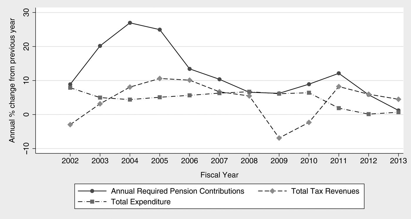
Figure 1. Volatility of required pension contributions vs. total state revenues and total expenditures.
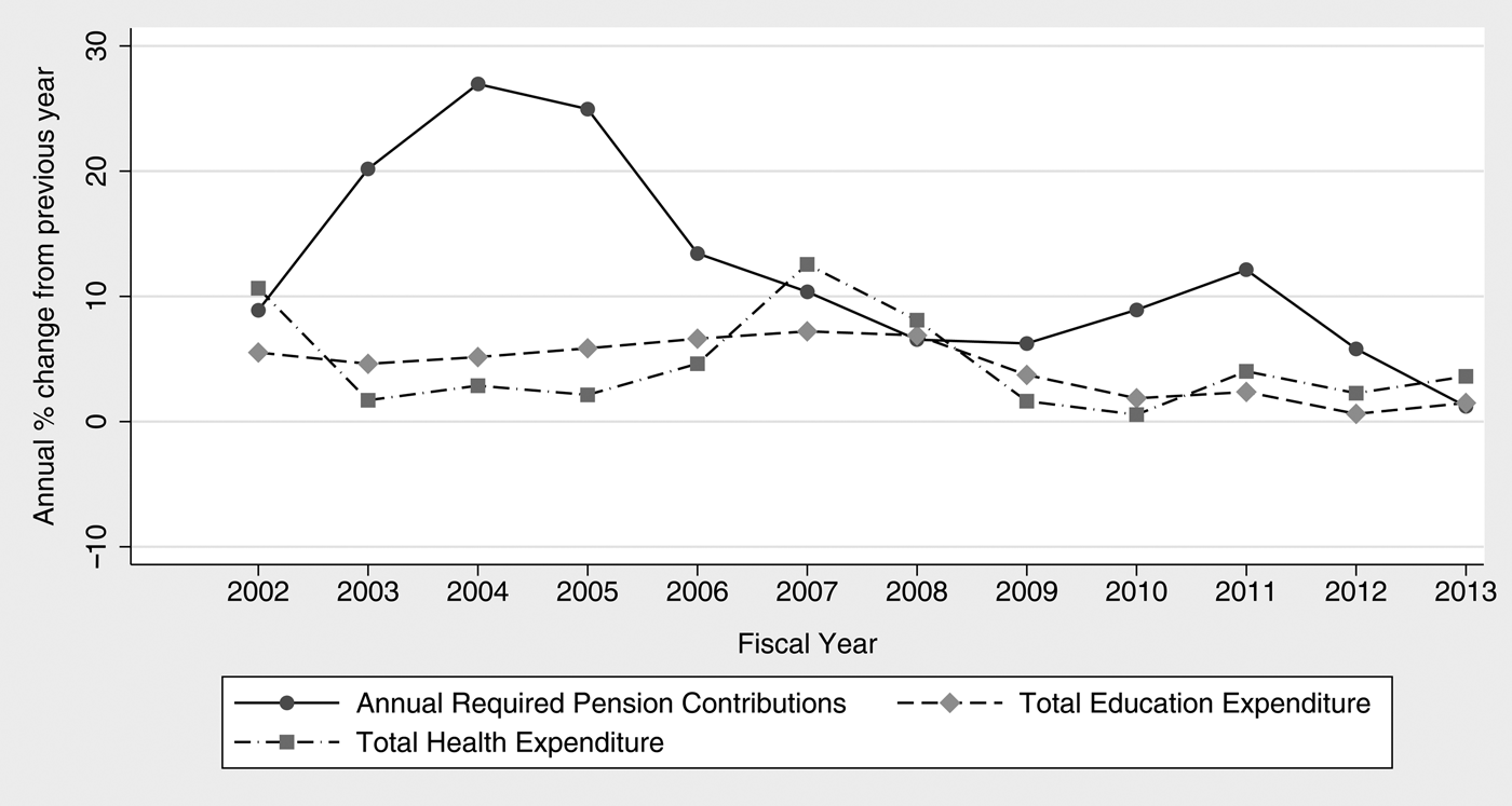
Figure 2. Volatility of required pension contributions vs. health and education expenditures.
Table 1. Year-to-year volatility
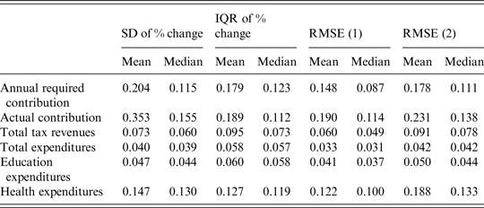
As is evident in Figure 1, there is more stability in the total revenues and expenditures across states than in required pension contributions, which decline from a growth rate of >20% in 2004 to approximately zero in 2013. This is also reflected in the numbers presented in Table 1. Actual pension contributions show greater volatility than the other fiscal categories as measured by the mean values of the SD and the IQR, with required contributions following in a close second. Only health expenditures come close, with a mean SD of 14.7 percentage points compared with 35.3 for the actual contribution. By contrast, total expenditures show a mean SD of 4.0 percentage points, consistent with the fact that overall state spending varies incrementally over time. When the median values are considered instead of the mean, the patterns remain somewhat consistent, though the volatility of health expenditures is now more comparable with that of pension spending, with a median SD of 13.0 percentage points, compared to 11.5 and 15.5 for required and actual pension contributions.
Since states typically use several prior years of data to conduct forecasts, it is possible that measuring the deviation from a trend may more closely reflect the amount of uncertainty in state estimates.Footnote 2 Using the RMSE from the first time-series model, actual pension contributions again show the most volatility, with a mean RMSE of 19.0 percentage points. Required contributions exhibit a mean of 14.8, while health expenditures and total tax revenues exhibit means of 12.2 and 4.1, respectively. The pattern of results from the second model is quite similar.
2.2 Contribution volatility and stabilization policies
The results from Table 1 highlight the fact that pension contributions showed significantly greater volatility than other expenditure categories, a finding that is consistent across numerous measures. To the extent that this poses a challenge to state budgeting, it is important to consider what is driving the fluctuations in actuarially determined contributions. Although large increases in required pension contributions are typically the result of investment shortfalls, the stabilization policies that states employ mean that a poor year of investment performance is not immediately reflected on a state's balance sheet nor does it translate immediately to an increase in required contributions.
Equation (3) demonstrates how the ARC is calculated. NCt represents the normal cost, the amount of future benefits earned by employees in the current year. The second term represents the current year's contribution toward the unfunded liability, which is equal to the difference between the actuarial value of plan assets and liabilities (AALt − Assett) divided by the amortization factor (a m).
Because the normal cost is fairly stable over time, large increases in the ARC are due primarily to the second term: actuarially accrued unfunded liabilities divided by the amortization factor. Amortization refers to the spreading out of repayment over a period of time. There are a number of dimensions along which amortizations methods vary, including whether they are open/closed, or level dollar/level percent of payroll, and the length of time of repayment. For example, if one focuses on the length of the amortization period, then the longer the amortization period, the lower the annual payments will be, and the longer it will take to pay off the liability.Footnote 3 As of 2013, about 45% of plans in the Public Plans Database had remaining amortization periods of 30 years or more, and another 45% had periods of 16–29 years (Boyd and Yin, Reference Boyd and Yin2016). Another crucial element of pension funding policy is asset smoothing, which refers to how market gains or losses are recognized. Typically, states smooth market gains or losses over a 5-year period, leading to a difference between the actuarial value of assets and liabilities and the market value. States that suffer an investment loss may not fully recognize the value of that loss until 5 years later. Conversely, states that see large investment gains are not able to immediately recognize the gains; while our discussion emphasizes the role of investment losses, smoothing does not always work in states’ favor.
Although a full discussion of stabilization policies is beyond the scope of this paper, the relevant point for our analysis is that market losses, increases in unfunded liabilities, and increases in required contributions do not occur simultaneously; in some cases it can be difficult to ascertain why contributions spiked in a given year, as they are often the result of a cascading number of events that occurred years earlier (see Boyd and Yin (Reference Boyd and Yin2016) for a recent discussion and for simulation illustrations. Also, as an illustrating example to which we return below, the Maryland Public Employees' and Retirees' Benefit Sustainability Commission (2011) shows how an investment return of −20% in 2009 did not translate to a spike in the state's required contribution until 2 years later). This is reflected in our data as well. While the size of the ARC is related to both the generosity of benefits as well as the level of unfunded liabilities, the change or fluctuation in the required contribution is not correlated with either.Footnote 4
Thus, the contribution volatility that we document occurs even after accounting for stabilization policies. Having described these fluctuations and discussed the link between investment risk and contribution volatility, we consider next the reforms that states have instituted in response to the financial pressures arising from DB plans.
3 State pension reform
3.1 Types of reform
Following the decline in assets values that occurred during the economic downturn and the ensuing focus on the fiscal ramifications for state governments, many states began to scale back their financial commitments to public DB plans. The changes that states made during this period took various forms, but we focus on three in particular: (a) increases to employee contributions, i.e., the payroll contributions that employees make toward their pensions, in contrast to the contributions made by their employer; (b) reductions in employee benefits; and (c) the replacement of DB plans with hybrid or defined contribution (DC) plans. These reforms primarily impacted future employees or those who were newly hired. The data on state pension reforms come from the National Conference of State Legislatures (2016), who have prepared annual summaries of state pension legislation.
Note that the first two types of reforms are not aimed at contribution volatility per se. In other words, we do not contend that states have necessarily responded to contribution volatility in the optimal way. The best way for states to reduce their exposure to market risk is to convert DB plans to DC plans; this shifts the risk from the state (the employer) to the employee. However, this option may not always be feasible for legal or political reasons. Alternative ways for states to reduce volatility are to implement more effective stabilization policies by, for example, increasing the amortization period, or shifting into safer asset categories, though these decisions may be in the hands of pension boards rather than the legislature and shifting into safer asset categories may be at odds with states’ desire to increase yield. Our hypothesis is merely that sharp fluctuations in required contributions are salient to legislators who face short-time horizons for re-election, and this influences their decision to engage in reform of some kind.
Figure 3 shows the number of states that increased employee contributions over the period 2001–2013, including states that legislated increases on more than one occasion. Unlike the state's contribution (as employer), which in most cases floats up and down based on the funding status of the plan, employee contribution rates are typically fixed as a percentage of payroll, with different classes of employees paying different rates based on the plan they are enrolled in. Making changes to these rates typically requires statutory adjustments. Because in some cases reforms were phased in over a period of years, and because our focus is on the factors that led states to engage in reform rather than the details of implementation, the figure reflects when the changes were enacted, not necessarily when they went into effect. The figure peaks in 2011 in the wake of the economic downturn, when 18 states increased employee contributions. This is consistent with our hypothesis, as there was a lag between when states saw steep investment losses (2008–2009) and when they saw an increase in their required contributions. Even prior to 2010, however, there were a few states each year that increased contributions; a smaller peak is visible in 2005.

Figure 3. Number of states increasing employee contributions.
Figure 4 shows the number of states that reduced benefits.Footnote 5 Reducing benefits can take many forms; we include both instances where the state tightened requirements for who was eligible to begin receiving or accruing benefits (vesting requirements), as well as instances where the state adjusted how benefits are calculated by reducing multipliers or cost-of-living adjustments. One common type of reform was to introduce a new tier of benefits for new employees with both higher eligibility standards and lower benefits. We do not include so-called ‘anti-spiking measures’ where the state passed legislation limiting the rate of increase in the final year salary since this legislation was more commonly aimed at abuses in the system rather than funding issues per se. Figure 4 shows a more consistent rate of increase in the amount of legislation than Figure 3, though both figures peak in 2011. Between 2001 and 2003 there was only one piece of legislation that reduced benefits in public pension plans. However, starting in 2004 there was a steady increase.Footnote 6
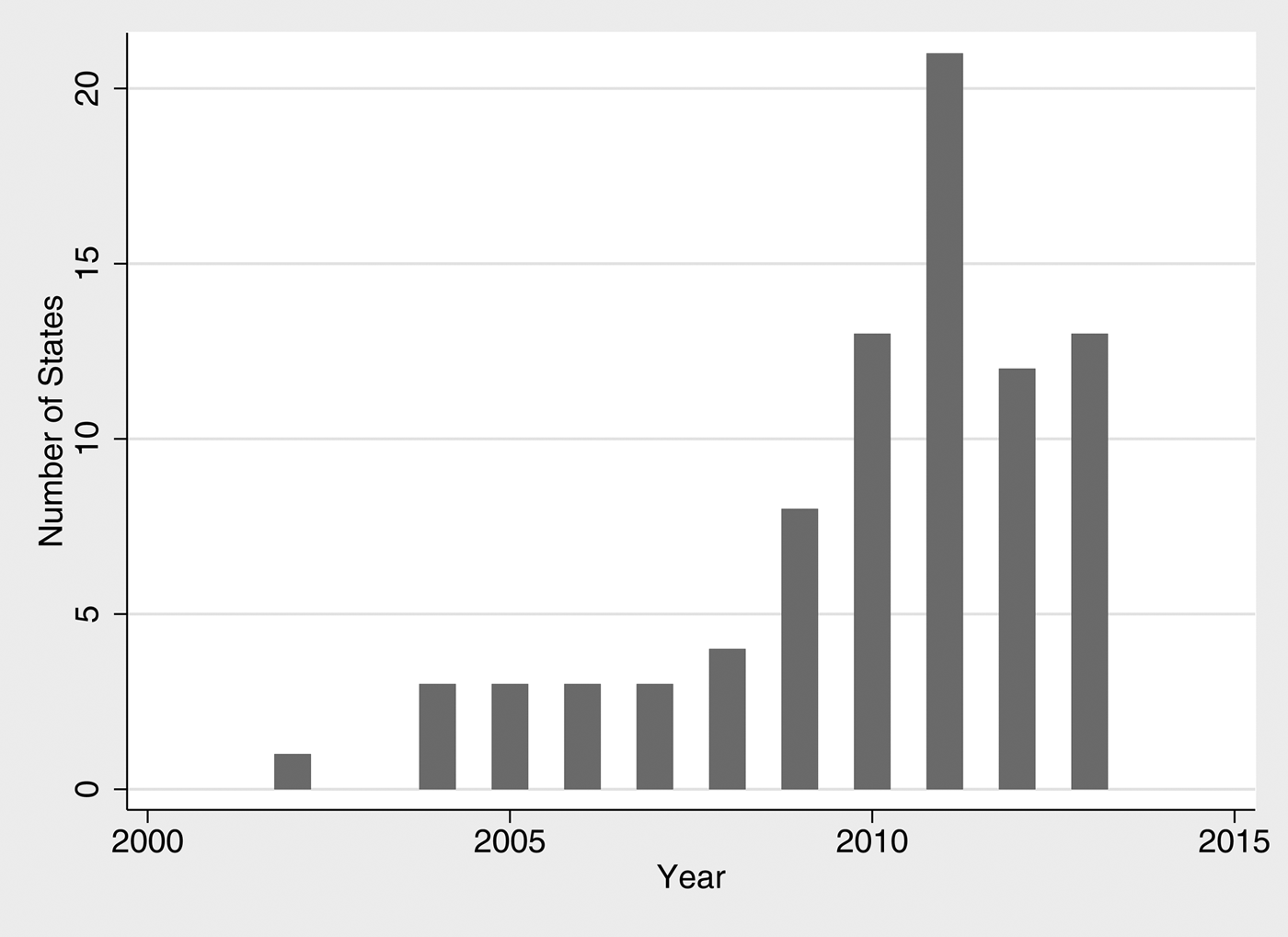
Figure 4. Number of states reducing benefits.
Figure 5 shows the number of states that closed a DB plan and replaced it with a hybrid or DC plan. Hybrid plans are pension plans that combine elements of DB plans with elements of DC plans, for example by layering a DC plan on top of a more modest DB plan.Footnote 7 We include only mandatory plans where employees did not have a choice whether or not to enroll in the new plan. A number of states have also introduced optional defined contribution or hybrid plans, though many of these changes were enacted by statute prior to 2001. As discussed by Munnell et al. (Reference Munnell, Aubry and Cafarelli2014), the motivations for these optional plans were different from the motivations that have led states more recently to introduce mandatory plans. Whereas the optional plans were intended to give employees the opportunity to take advantage of a rising stock market, the mandatory plans have been introduced for reasons of financial exigency on the part of the state.Footnote 8 As the figure makes clear, the number of states that have closed DB plans remains small relative to the number of other reforms that have taken place.

Figure 5. Number of states replacing a DB plan with a hybrid or DC plan.
3.2 Factors in reform
There is little research examining the determinants of reform. The only study we are aware of is Munnell et al. (Reference Munnell, Aubry and Cafarelli2014), who look at the factors influencing the probability of introducing a DC plan (optional or otherwise). The authors use a linear probability model and separately examine the pre- and post-crisis periods, finding that the most significant factor in introducing a DC plan is Republican control of the government, though they also find that in the post-crisis period the extent of unfunded liabilities and the generosity of the plans were also contributing factors. As noted above, part of the authors’ motivations for examining separately the pre- and post-crisis periods is that the rationale for introducing optional DB plans prior to the financial crisis was distinct from the rationale for introducing mandatory plans after the crisis. Nevertheless, their analysis is limited by the relatively small number of states that have introduced DC plans. The authors also confine their analysis to a simple panel data analysis rather than employing event history methods to better understand the duration of the pre-reform period.
Munnell et al. (Reference Munnell, Aubry and Cafarelli2014)’s analysis suggests that both the generosity of benefits as well as the size of unfunded liabilities are correlated with reform. Unlike their study, we focus specifically on the role of contribution volatility. Though states with generous benefits and large unfunded liabilities will face high levels of contributions over time, fluctuations in the required contributions will not occur directly in tandem with fluctuations in investment returns; as previously discussed, various stabilization policies ensure that investment losses are not factored immediately into required payments.
Although contribution volatility must be considered separately from the size of the UAAL (unfunded actuarial accrued liability), any model that attempts to uncover the determinants of pension reform must account for both the generosity of benefits as well as the size of the UAAL. The question that we focus on is whether, even after accounting for these factors (and further covariates that we discuss below), contribution volatility is a significant determinant of pension reform. Given that the volatility associated with pension spending appears greater than the volatility associated with other large categories of state spending – and that this factor may even be more salient to state legislators than the size of unfunded liabilities – we hypothesize that these short-term fluctuations in pension contributions have been a significant factor in states’ decisions to adopt reforms to their pension systems.
4 Descriptive findings
To further motivate our analysis, we first present some descriptive findings. We begin with a simple cross-sectional comparison of plans that underwent reform and those that did not. These naive comparisons do not account for the many factors discussed above nor do they fully account for the multi-level structure of the data; we present them merely as descriptive evidence to further investigate our hypothesis. Table 2 compares the median volatility (using all four metrics introduced above) of plans that underwent reform at some point between 2001 and 2013 and those that did not.Footnote 9 For benchmarks, we also include comparisons of the median funded ratio (averaged over the sample period) and the median generosity of benefits. While only one of the volatility estimates is statistically significant, every single estimate is positive, indicating that reform plans had higher volatility than plans that did not undergo reform. Both the funded ratio and the generosity of benefits (average benefits/average salary) have the expected signs for the most part – plans that underwent reform were lower funded and more generous – though generosity is negative in one of three estimates. So while pension reform is associated with larger unfunded liabilities (lower funded ratios), it also appears to be associated with greater contribution volatility.
Table 2. Cross-sectional comparison of plans that did and did not undergo reform

Legend: †p < 0.10. N = 114 plans. The estimates reflect the difference between the median values for plans that introduced a reform sometime between 2001 and 2014 and those that did not. Every volatility estimate is positive, indicating that plans that underwent reform had greater volatility than those that did not.
While Table 2 presents cross-sectional comparisons, it is helpful to also examine variation over time, and specifically the fiscal changes that occurred just prior to or simultaneously with reform. Table 3 includes only those plans that saw a reform and examines the extent to which the year of the first reform coincided with the largest spike in the contribution rate that a plan experienced over the sample period. The intent is to discover whether sharp changes in the ARC coincided with reform. As a benchmark, the table also looks at the extent to which reforms coincided with the plan's lowest funded ratio.
Table 3. Probability of first reform

Legend: *p < 0.05, †p < 0.10. The table looks at the first year that a reform occurred and examines the extent to which the first reform corresponded with either (a) the largest increase in the contribution rate, or (b) the lowest funding ratio over the period of study. The sample only includes plans that underwent a reform. The estimates come from a linear probability model with plan and year fixed effects. The dependent variable is an indicator variable for the year in which the plan first enacted reform.
The table shows that there was a positive correlation between the largest spike in a plan's contribution rate and the first reform. The probability of reform increased by 6.4 percentage points in the year of a plan's largest contribution increase. This correlation is positive whether one looks at any type of reform or the two more narrow types of reform: increases to employee contribution rates and benefit reductions. On the other hand, there is less consistency to the correlation between the year of first reform and the low point of a plan's funded ratio. Two of the three coefficients are negative, implying that the lowest funding ratio was negatively associated with the probability of reform.
As one final piece of evidence, we present the state of Maryland as an illustrative example. Both of Maryland's state-wide pensions systems increased employee contributions and reduced benefits in 2011. As Figure 6 makes clear, these reforms coincided with a sharp increase in the size of the state's required contribution. Notably, this increase in the required contribution occurred 2 years after a sharp drop in the state's aggregate funded ratio. In fact, the state's investments had rebounded strongly in 2010, earning a 14.0% return after earning returns of −5.4% and −20.0% in 2008 and 2009, respectively (Maryland Department of Legislative Services, 2011).Footnote 10 Furthermore, media reports at the time called attention to the immediate budgetary pressures the states was facing (Davis and Wagner, Reference Davis and Wagner2011). While not every state demonstrates such clear correspondence between spikes in its contribution rate and the enactment of pension reform, Maryland's pension accounting – as well as the rest of the descriptive evidence presented above – suggest that a jump in the size of a state's ARC may contribute to the likelihood of reform.
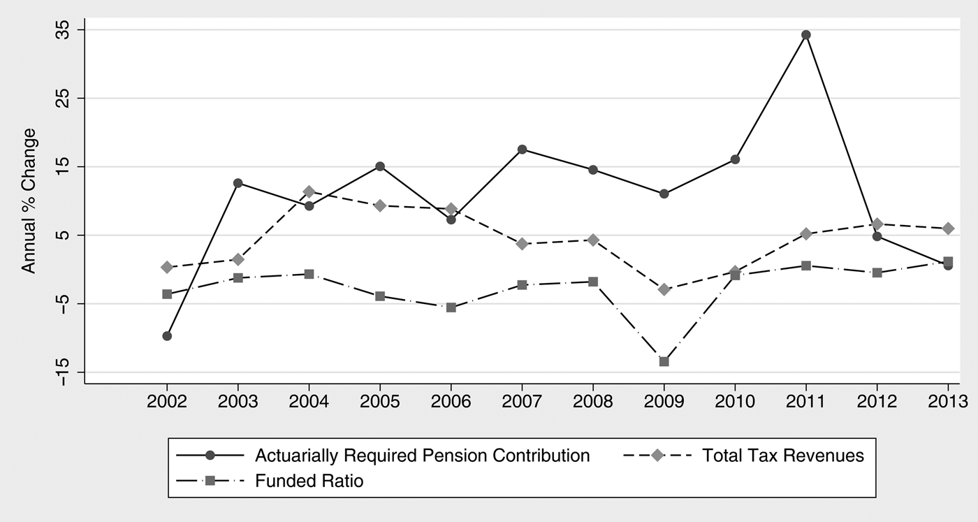
Figure 6. Maryland.
5 Methods
To examine in a more rigorous fashion the role of contribution volatility, we employ both panel data and survival methods. Our panel data analysis looks at the probability that a pension plan underwent reform in a given year. The dependent variable is a one in the case that a reform occurred and zero otherwise; we utilize a logit model to account for the binary nature of the dependent variable. We do not censor any observations since in some cases reforms occurred on multiple occasions affecting the same plan. To account for unobserved heterogeneity, we use state and year fixed effects, which result in the loss of states that do not enact a reform at any point during our study period since there is no within-state variation in the dependent variable. (There are three states that never implement any reform.)Footnote 11 However, all states are included in the survival analysis that follows. We do not split our sample into pre- and post-reform periods the way that Munnell et al. (Reference Munnell, Aubry and Cafarelli2014) do since our analysis does not include optional DC plans. We do however include year fixed effects to account for year-specific shocks.
We also use survival methods. Survival models – or duration models – analyze how long a particular entity remains in a steady state before some event occurs. This requires examining the hazard rate, the risk to an entity of having its steady state interrupted in some period, given that the entity has persisted in the steady state for certain length of time (Box-Steffensmeier and Jones, Reference Box-Steffensmeier and Jones2004). In this case, the event of interest is a pension reform, and the model examines the length of time before a pension plan introduces a reform. Our primary interest is in the time before the first reform; given that many states later introduced legislation that made modifications to their initial reforms, we believe the factors that led to the first reform were in many cases the most significant. In the single failure model, we drop any observations following the first reform. However, we also present results for a multiple failure model that includes all reforms. Hence, while our fixed-effect approach considers multiple reforms, but excludes plans that do not undergo reform, the single-failure survival analysis includes all plans but does not include observations following the first reform. The multiple failure model includes all observations. In the case that a plan never experiences a reform, it is ‘right-censored’ in the duration models; in other words, the duration time only provides information up to the last year in the sample.
The choice of survival model depends in part about assumptions regarding the baseline hazard rate, i.e., the hazard rate when all covariates are zero. There are multiple parametric models that assume a particular parametric form for the baseline hazard rate; however, these models require strong assumptions about the survival function. As is common in the applied literature, instead of a parametric approach, we employ the Cox proportional hazards model, a semi-parametric approach that makes no assumptions about the baseline hazard rate.
We examine three different outcomes based on the reforms discussed in Section 3 above. Each outcome is a binary variable, taking on a value of one in the case that: (1) a state required employees to increase their contributions to the plan, (2) a state reduced benefits to plan beneficiaries, and (3) a state introduced either of the above two reforms or closed the DB plan and replaced it with a hybrid or DC plan. We chose to look at ‘any reform’ as the third outcome – rather than simply looking at the introduction of hybrid/DC plans – because the small number of plans that fall into that category compromises statistical power. Furthermore, insofar as an increase in employee contributions and a reduction in benefits are equivalent, this category more comprehensively reflects the desire on the part of the legislature to reduce the exposure to fiscal pressures related to DB plans. As noted above, our observations are at the plan-year level, unlike Section 2 when we aggregated plans to the state level so as to examine state-level spending patterns. To account for the fact that some of our variables show variation at the state-level rather than the plan-level, we cluster our standard errors at the state level.
To properly isolate the variable of interest, we also control for other factors that may plausibly lead states to engage in reform. Table 4 provides summary statistics. Based on the Munnell et al. (Reference Munnell, Aubry and Cafarelli2014) analysis, we include the amount of unfunded liabilities as a percentage of payroll, average benefits as a proportion of the average salary, a binary variable expressing whether or not a government was Republican-controlled, and a binary variable indicating whether employees in the plan are also covered by Social Security. Plans with a large amount of unfunded liabilities as a percentage of covered payroll will be more likely to reform a plan as a result of the financial difficulties that it poses. Similarly, generous plans – as captured by the proportion of average benefits divided by average salary– may be targets for reform since the employer may be making large contributions, even if the plan is fully funded.Footnote 12 If the workers of a plan are also covered by Social Security, they may be less adversely affected by reforms than if they relied on the pensions benefits alone for their retirement income. In addition to these covariates, we also include the unemployment rate as a proxy for the economic condition of the state. Finally, as a robustness check, in one specification we include the change in, rather than the level of, unfunded liabilities as a percentage of payroll in case it is the change rather than the level that is the driving factor.Footnote 13
Table 4. Summary statistics

As discussed above, there are various metrics for measuring contribution volatility. In our regression analysis, because of the panel nature of the data, the independent variable of interest is the deviation in a given year. Although the time-series models enable us to calculate the deviation from trend, one downside to these approaches is that they do not enable us to include measurements from the early years of our sample, compromising the precision of our estimates. Thus, we use the annual percent change as a simple measure (used above in the descriptive results) since it can be measured for all years. However, to ensure that our results are robust to the choice of metric, we also estimate the results using the other two measures, though we expect that these results will have less power due to the smaller number of observations.Footnote 14
6 Results
The results are presented in Tables 5–7. Table 5 presents the results for any type of reform. Table 6 looks at the increase in employee contributions. Table 7 looks at the reduction in benefits. In all of the tables, the first two columns show the fixed effects results. The third and fourth columns show the results from the survival models. All the continuous coefficients have been standardized, so that a one unit increase corresponds to one SD. All the binary variables (Republican controlled government, Covered by Social Security) remain as zeros and ones. The coefficients in the panel data models indicate the relationship between the independent variables and the log-odds of a reform occurring. A positive coefficient indicates that an increase in the independent variable increases the likelihood of a reform in a given year. For the coefficients in the survival models, a positive coefficient indicates that the hazard is increasing as a function of the covariate (and hence, the duration of time prior to reform is shorter).
Table 5. Any reform
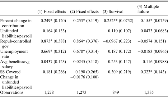
Legend: **p < 0.01, *p < 0.05. Standard errors clustered at the state level. Fixed-effect regressions include state and year fixed effects.
Table 6. Increases in employee contributions
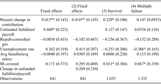
Legend: **p < 0.01, *p < 0.05. Standard errors clustered at the state level. Fixed-effect regressions include state and year fixed effects.
Table 7. Reductions in employee benefits
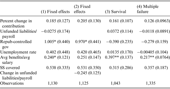
Legend: **p < 0.01, *p < 0.05. Standard errors clustered at the state level. Fixed-effect regressions include state and year fixed effects.
In Tables 5 and 6, the variable of interest – the percent change in contributions – is positive and statistically significant in all but one specification. Across all the tables, the coefficient is larger than the coefficient on unfunded liabilities with one exception. The change is unfunded liabilities is never significant and log-likelihood tests reveal that the model fit does not improve as a result of including it. As hypothesized, sharp increases in the required contribution seem to be a major determinant of state pension reform and the regressions indicate that they may play a more significant role than the extent of unfunded liabilities.
In Table 5, only three other variables obtain statistical significance in any of the models: Republican-controlled government, the unemployment rate, and whether employees are covered by Social Security. All have the expected sign; reforms are more likely to occur with Republican-controlled governments and in states where the unemployment rate is higher; plans where employees are also covered by Social Security increased employee contributions sooner than other plans. In Table 6, the results are broadly similar. In the first column of Table 6, the extent of unfunded liabilities as a percent of payroll is significant and has a larger coefficient than the percent change in the required contribution. However, this is the only specification where that is the case. In Table 7, the variable of interest is not statistically significant, but the coefficients still carry the expected signs and are only slightly smaller in magnitude. The only variable to obtain statistical significance in both the fixed effects and the survival models in Table 7 is the generosity of benefits. This result appears reasonable: plans that offer more generous benefit packages are more likely to reduce benefits and do so earlier. It may be the case that benefit reductions are driven primarily by the generosity of the benefits.
To ensure that the results are robust to the measure of volatility, Table 8 present results using the deviation from trend (from Model 1) rather than simply the annual percent change of the required contribution. The table reports only the coefficient on the main explanatory variable and omits the coefficients from other covariates. As noted above, this alternative measure of volatility requires losing some observations from the early years of the sample. The results are very consistent with those of Tables 5–7, though the standard errors are slightly larger. The estimates for any reform and for increased contributions are statistically significant in multiple specifications. The estimates for reduced benefits are slightly larger than the corresponding estimates in Table 7. We do not report the results using the deviation from trend from Model 2, but these too yield similar results.
Table 8. Results using an alternative measure of volatility

Legend: *p < 0.05. The table reports the estimated coefficient on the deviation from trend, where the deviation is calculated using equation (1). The specifications are otherwise identical to those in Tables 5–7. For the first row, the dependent variable is equal to 1 in the case of any reform, as in Table 5. For the second and third rows, the dependent variable takes a value of 1 in the case of an increase in contributions and a reduction in benefits, respectively, as in Tables 6–7.
One further robustness check that is necessary with the Cox model is to ensure that the proportional hazard assumption is not violated. We test the null hypothesis of non-proportional hazards using the Schoenfeld residuals in the multiple-failure model examining all reforms. We are unable to reject the null (p-value of 0.67 on the variable of interest, 0.21 on the global test), indicating that the model does not show evidence of non-proportional hazards and that the use of the Cox model is appropriate.
7 Discussion
In the wake of the economic downturn of 2008–2009 and the sharp decline in asset values, there has been considerable discussion of the large unfunded liabilities that have appeared in US public pension plans. These liabilities are regarded as a threat to the long-term fiscal sustainability of state and local governments and have spurred various discussions about how to address the shortfalls.
In this paper, we argue that while these shortfalls are important, in the short term it is the sudden increases in required pension spending and not just the size of the liabilities that have led to reform proposals. Spikes in pension costs typically do not occur simultaneously with investment shortfalls due to stabilization policies that spread out and defer unfunded liabilities. As a result, legislators with short time horizons for re-election must confront highly salient cost increases that are in some cases the result of investment shortfalls from many years prior.
First, we described how the volatility of pension spending compares to the volatility of other tax and spending measures. Next, we summarized the types of pension reforms that states have introduced, focusing on legislation that: either (1) increased employee contributions, (2) reduced benefits, or (3) replaced DB plans with hybrid or DC plans. We used both fixed effects and survival models. In all but one of our specifications, contribution volatility showed a coefficient that was larger than the covariate depicting the relative size of the unfunded liabilities. It appears that spikes in the amount of a state's required contribution have some impact on the decision to engage in reform, and this factor may even have more explanatory power than the size of unfunded liabilities. On the other hand, our findings regarding benefit reductions do not point to contribution volatility as a leading factor. Instead, benefit reductions may be more closely related to the generosity of a plan's benefits.
Our results are not without caveats. Any analysis that looks to uncover the motivations behind state legislators’ decision-making is necessarily prone to oversimplification. We do not contend that contribution volatility is the sole reason for pension reforms. Rather, our argument is that contribution volatility is a factor that may have led states in the direction of reform, and has also been somewhat overlooked. When looking at the entire set of state-wide plans, it shows higher correlation with reform than other factors that have received widespread attention.
In some cases, states may have taken several years to consider reform proposals before enacting any type of reform. If a state began to consider reform proposals as a result of, for example, unfunded liabilities in one year, but did not enact reform until several years later, then our models may misstate the true drivers of reform. Nevertheless, the consistency of our findings across a variety of descriptive and multivariate models lends some credence to our results.
Another caveat is that, as Figure 1 makes apparent, many states saw fluctuations in their contributions in 2001–2004, even prior to when many reforms were occurring. Further descriptive analysis (not shown) indicates that for many states, it was their second or third spike in contributions that precipitated reform, and not necessarily their first. The political environment may not have been right in the early 2000s for states to address pension spending. When pension contributions spiked again in the wake of the economic downturn as states were finally forced to reckon with investment shortfalls that had occurred, the political environment may have been more receptive to reform.
One question that arises in response to our analysis is how states should address fluctuating contributions. States have already attempted to stabilize their contributions by amortizing the unfunded liability over long periods of time, as well as by smoothing the recognition of assets. GASB 67/68 have placed some restrictions on these practices, and so states will have less discretion than in the past. Another alternative of course is for states to shift away from DB plans. This is the most obvious way for employers to shift risk on to employees, though states must also consider the implications for employee retention and recruitment (Clark et al., Reference Clark, Hanson and Mitchell2016).
In light of our results, we argue that future discussions of public pension funding should take note not only of the extent of unfunded liabilities, but also the short-term risk that pension spending poses for state governments. Given the short-term focus of many state legislators, it is this uncertainty that may represent the larger factor in their decision-making processes.
Acknowledgements
We are grateful to seminar participants at the 2016 Association for Policy Analysis and Management conference, 2016 National Tax Association conference, and 2015 Association for Budgeting and Financial Management conference for their feedback on earlier drafts. David Matkin, Gang Chen, and two anonymous referees also provided helpful comments.

