1. Introduction
In large-eddy simulation (LES) of high Reynolds number wall-bounded turbulent flows occurring in industrial and environmental applications, a wall model (Piomelli & Balaras Reference Piomelli and Balaras2002; Bose & Park Reference Bose and Park2018; Goc, Moin & Bose Reference Goc, Moin and Bose2020; Yang et al. Reference Yang, Milliren, Kistner, Hogg, Marr, Shen and Sotiropoulos2021) is necessary even on the state-of-the-art supercomputers, which models the flows in the near-wall region to avoid the need to resolve the small-scale turbulence structures therein (Choi & Moin Reference Choi and Moin2012; Yang & Griffin Reference Yang and Griffin2021). The existence of universality for the near-wall flow is beneficial for such treatments, which, however, is not yet observed for all types of turbulent flows especially for those under non-equilibrium states. This makes the traditional wall models based on the equilibrium hypothesis unable to accurately simulate non-equilibrium flows, such as flows with separation (Breuer, Kniazev & Abel Reference Breuer, Kniazev and Abel2007; Duprat et al. Reference Duprat, Balarac, Métais, Congedo and Brugiére2011). The machine learning method offers a novel avenue for constructing models for non-equilibrium flows. Nonetheless, the acquired models frequently face challenges related to limited generalizability and suboptimal a posteriori performance (Zhou, He & Yang Reference Zhou, He and Yang2021a; Zhou et al. Reference Zhou, Yang, Zhang and Yang2023b). In this study, we introduce a features-embedded-learning (FEL) wall model for LES of separated flows. The model enhances generalizability by leveraging high-fidelity data from separated flows and the law of the wall. The a posteriori performance is enhanced through embedded learning using the ensemble Kalman method.
Lack of generalizability is one of the most critical problems for data-driven turbulence models, although much effort has been put in for both Reynolds-averaged Navier–Stokes methods (Ling, Kurzawski & Templeton Reference Ling, Kurzawski and Templeton2016; Zhu et al. Reference Zhu, Zhang, Kou and Liu2019; Zhao et al. Reference Zhao, Akolekar, Weatheritt, Michelassi and Sandberg2020; Wu, Cui & Xiao Reference Wu, Cui and Xiao2022; Zhang et al. Reference Zhang, Xiao, Luo and He2022a; Lyu, Kou & Adams Reference Lyu, Kou and Adams2024) and LES methods (Maulik et al. Reference Maulik, San, Rasheed and Vedula2019; Park & Choi Reference Park and Choi2021; Kang, Jeon & You Reference Kang, Jeon and You2023; Wang, Yuan & Wang Reference Wang, Yuan and Wang2023; Xu et al. Reference Xu, Wang, Yu and Chen2023). Employing neural networks to model near-wall flows dates back to the work by Milano & Koumoutsakos (Reference Milano and Koumoutsakos2002). In wall-modelled LES (WMLES), approximate boundary conditions, such as the shear stress at the wall, define how the near-wall unresolved flow structures influence the outer flow. In traditional wall models, the wall shear stress is often computed using the law of the wall (Deardorff Reference Deardorff1970; Werner & Wengle Reference Werner and Wengle1993) or by solving the thin-boundary-layer equation (Cabot & Moin Reference Cabot and Moin2000; Wang & Moin Reference Wang and Moin2002; Park & Moin Reference Park and Moin2014; Yang et al. Reference Yang, Sadique, Mittal and Meneveau2015a). In the work by Yang et al. (Reference Yang, Zafar, Wang and Xiao2019), a feedforward neural network (FNN) model was constructed to compute the wall shear stress using the flow quantities at the first off-wall grid nodes, and successfully applied to WMLES of turbulent channel flows at various Reynolds numbers and spanwise rotating turbulent channel flows (Huang, Yang & Kunz Reference Huang, Yang and Kunz2019). In the model developed by Lee, Lee & Lee (Reference Lee, Lee and Lee2023), the input features are extracted from the Fukagata–Iwamoto–Kasagi identity (Fukagata, Iwamoto & Kasagi Reference Fukagata, Iwamoto and Kasagi2002) to describe the effects of flow dynamics on the wall shear stress. It was shown that incorporating known physics in the construction of input features improves the model generalizability for different Reynolds numbers (Yang et al. Reference Yang, Zafar, Wang and Xiao2019; Lee et al. Reference Lee, Lee and Lee2023). Generalization of a data-driven wall model for different flow regimes is even more challenging. One idea is to build the model using data from various flows, which can be in the same flow regime but with different parameters or in different flow regimes. To simulate shock–boundary layer interaction, Bhaskaran et al. (Reference Bhaskaran, Kannan, Barr and Priebe2021) trained a wall model using the data from eight wall-resolved LES (WRLES) cases with different curvatures near the blade trailing edge and different shock locations and strengths. To simulate supersonic turbulent flows with separation, Zangeneh (Reference Zangeneh2021) trained a wall model using data from the zero-pressure-gradient turbulent flow over a flat plate and supersonic flow around an expansion–compression corner. To simulate separated flows, Dupuy, Odier & Lapeyre (Reference Dupuy, Odier and Lapeyre2023) trained a wall model using the filtered high-fidelity data from turbulent channel flow, the flow in a three-dimensional (3-D) diffuser and the backward-facing step flow. Assuming that the flow in the near-wall region can be modelled using a finite set of canonical flows, Lozano-Durán & Bae (Reference Lozano-Durán and Bae2023) proposed a building-block-flow wall model, tested the model for canonical flows and applied it to two aircraft configurations. The lack of the law of the wall means that the state of flow at a single off-wall grid node is not enough to fully describe the near-wall flow for separated flows. Zhou et al. (Reference Zhou, He and Yang2021a) employed the velocity and pressure gradient at three off-wall grid nodes as input features to construct a neural network model for computing wall shear stress, which was trained using the wall-resolved data of the periodic hill flow. The predicted instantaneous wall shear stress agrees well with the reference data with the correlation coefficients higher than 0.6. To improve the generalizability of the model, the law of the wall was later introduced in the training of the model (Zhou et al. Reference Zhou, Yang, Zhang and Yang2023b), showing good performance for both the periodic hill flow and the turbulent channel flow.
Suboptimal a posteriori performance remains as a challenge for data-driven wall models especially for non-equilibrium flows. One main cause is the inconsistency in the environments for model training and prediction (Duraisamy Reference Duraisamy2021). This mainly includes the numerical discretization error (which is small in wall-resolved simulations while is large in coarse-grid WMLES) and the error from the subgrid-scale (SGS) modelling (which is zero or small in wall-resolved simulations while it may become significant in WMLES). To address this problem, efforts have been made in the way of preparing the training data and using different machine learning methods. In the work by Lozano-Durán & Bae (Reference Lozano-Durán and Bae2023), the training data were generated from the so-called E-WMLES, in which the ‘exact’ SGS model and wall shear stress are employed to match the mean velocity profiles from direct numerical simulation (DNS). Performance better than the model based on filtered DNS data was obtained. In the work by Bae & Koumoutsakos (Reference Bae and Koumoutsakos2022), the multi-agent reinforcement learning was employed to train a wall model in a WMLES environment for turbulent channel flows. In the proposed model, the agents are evenly distributed points on the wall with their actions of adjusting the applied wall shear stress and the rewards based on the predicted wall shear stress. Later development of the model based on reinforcement learning to consider pressure gradient effects was also carried out (Zhou et al. Reference Zhou, Whitmore, Griffin and Bae2023a; Zhou & Bae Reference Zhou and Bae2024b). Possible sources of errors for wall models based on different machine learning methods were analysed by Vadrot, Yang & Abkar (Reference Vadrot, Yang and Abkar2023).
The wall shear stress boundary condition is often employed to approximate the effects of the unresolved near-wall flow structures on the outer flow in WMLES. However, it may become insufficient for separated flows for which a constant shear layer is lacking. Specifically, for the flow near the separation or reattachment point, the amplitude of wall shear stress is small in the region, but there still exist small-scale near-wall flow structures acting on the outer flow, which cannot be captured by the wall shear stress boundary condition. Moreover, the poorly computed SGS stresses at the first off-wall grid nodes further complicates the modelling of separated flows.
In this work, we propose to enable the generalization ability of the neural network wall model by integrating high-fidelity data and knowledge and improve the a posteriori performance by accounting for the SGS modelling defect in an embedded-learning environment. The proposed wall model is composed of a model for wall shear stress and a model for the eddy viscosity at the first off-wall grid nodes, in which the latter is trained in a WMLES environment, and the former is trained using the separated flow data and the law of the wall. Such a training approach prevents contaminating the wall shear stress model with errors in WMLES.
The rest of the paper is organized as follows: the proposed wall model is introduced in § 2; the training of the model is described in § 3; systematic assessment of the proposed model in the periodic hill flows is presented in § 4; the physical interpretation for the proposed model is in § 5; the application of the proposed model to other flow configurations is presented in § 6; the conclusions are drawn in § 7.
2. The FEL wall model
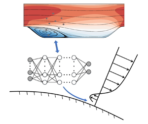
The FEL wall model approximates the effects of near-wall flows on the outer flow using wall shear stress and eddy viscosity at the first off-wall grids. The former (dubbed as ‘$\text {FEL}_{\tau _w}$’) is computed using a neural network model trained separately using high-fidelity data and the law of the wall. The model for the latter (dubbed as ‘$\text {FEL}_{\nu _t}$’) is trained in an embedded way in the WMLES environment to account for the SGS modelling issue for separated flows. A schematic of the FEL wall model is shown in figure 1.
2.1. Wall shear stress model
We empower the capability of the neural network model in estimating wall shear stress for different flow regimes using the data from separated flows and the law of the wall. Specifically, the data from the periodic hill flow and the logarithmic law for the mean streamwise velocity profile, which is introduced in Appendix A, are employed for training the wall shear stress model. The periodic hill case, even though its geometry is relatively simple, contains several flow regimes, i.e. flows with pressure gradients, flow separation and flow reattachment. The inclusion of the logarithmic law in model training then enables the trained model to react properly to flows in the equilibrium state.
A FNN is employed for building the connection between the near-wall flow and the wall shear stress. The neural network comprises an input layer, six hidden layers with 15 neurons in each layer and an output layer. The hyperbolic tangent (tanh) function serves as the activation function. The input features consist of six flow quantities at three wall-normal points, with the distance between two adjacent points denoted as $\Delta y_n/\delta _0 = 0.03$,
where $y_n$ is the wall-normal distance, $u_{w,t}$, $u_{w,n}$ and $u_s$ are the velocity components in the wall-tangential, wall-normal and spanwise directions, ${\partial p}/{\partial w_t}$, ${\partial p}/{\partial w_n}$ are the pressure gradients in the wall-tangential and wall-normal directions, $u_b$ is the bulk velocity, $\delta _0$ is the global length scale. It is noted that the length scale $\delta _0$ represents the scale of the outer flow. It is set as the hill height $h$ in periodic hill flows, and the half-channel width $\delta$ in turbulent channel flows. For flows in a complex geometry with several geometric length scales, a systematic way for defining the length scale is yet to be developed. A case-by-case approach is probably needed. The wall-normal distance is normalized by a near-wall length scale $y^{*} = \nu /u_{\tau p}$ (Duprat et al. Reference Duprat, Balarac, Métais, Congedo and Brugiére2011), where $\nu = \mu /\rho$ is the kinematic viscosity, $u_{\tau p} = \sqrt {u_{v}^2+u_p^2}$, $u_{v} = \sqrt {| {\nu u_{w, t}}/{y_n} |}$, $u_p = | ({\nu }/{\rho } )({\partial p}/{\partial w_t}) |^{1/3}$. The output labels are the wall-tangential and spanwise wall shear stresses,
The cost function is defined as the mean square error between the predicted output and the real output. The error backpropagation scheme (Rumelhart, Hinton & Williams Reference Rumelhart, Hinton and Williams1986) implemented with TensorFlow (Abadi et al. Reference Abadi2016) is employed to train the $\text {FEL}_{\tau _w}$ model by optimizing the weight and bias coefficients to minimize the cost function. A detailed description of the training procedures can be found in Zhou et al. (Reference Zhou, He and Yang2021a).
2.2. Eddy viscosity model
The SGS modelling error and discretization error are the two major causes for the suboptimal a posteriori performance of a data-driven wall model in a WMLES environment. In separated flows, a near-wall layer of constant shear stress does not exist. In WMLES, the near-wall layer, which is in a non-equilibrium state for separated flows, is not resolved by the grid. The wall shear stress boundary condition alone is not enough to model the way the unresolved near-wall flow affects the outer flow. In this work, we postulate that a proper eddy viscosity can approximate the effects of the near-wall flow not captured by the wall shear stress, and accounts for the SGS modelling error and discretization error in the meantime.
There are several options to establish an eddy viscosity model, e.g. an analytical approach, a data-driven approach or a hybrid approach. To compromise between generalizability and predictive capability of the model, a hybrid approach is employed. Specifically, we employ a modified version of the mixing length model with its coefficients learned in an embedded way, in the following form:
where the von Kármán constant $\kappa \approx 0.4$, $D = [ 1 - \exp (-(y^+ / A^+)^3) ]$, $A^+=25$, $y^+ = y_n u_\tau /\nu$, $u_\tau = \sqrt {\tau _w/\rho }$ is the friction velocity given by the wall shear stress model in § 2.1. With (2.3), the eddy viscosity at the first off-wall grid node is modelled using the modified mixing length model instead of the dynamic Smagorinsky model (DSM) employed in the outer flows. The exponential form coefficient, i.e. $\exp ( E_\nu ({u_p}/{u_{\tau p}}))$ is proposed to prevent negative eddy viscosity. While a clipping procedure for negative $\nu _t$ can be employed as well (Zhou et al. Reference Zhou, He, Wang and Jin2019; Park & Choi Reference Park and Choi2021), it may affect the predictive capability of the model.
To approximate the modified mixing length model using a neural network, the model coefficient $E_\nu$ is used as the output label. The neural network is composed of an input layer, six hidden layers with 15 neurons in each layer and an output layer. In the input layer, the input features are the same as those for the wall shear stress model, i.e. (2.1). The hyperbolic tangent (tanh) function is also employed as the activation function for this new neural network. Using the ensemble Kalman method, the $\text {FEL}_{\nu _t}$ model is trained in the WMLES environment in an embedded way.
2.3. Ensemble Kalman method
The ensemble Kalman method is a statistical inference method based on Monte Carlo sampling, and has been widely used in various applications (Chen et al. Reference Chen, Chang, Meng and Zhang2019; Zhang et al. Reference Zhang, Xiao, Gomez and Coutier-Delgosha2020; Schneider, Stuart & Wu Reference Schneider, Stuart and Wu2022; Zhang et al. Reference Zhang, Xiao, Wu and He2022b; Liu, Zhang & He Reference Liu, Zhang and He2023). In this work, the method is employed to learn the weights in the neural network model for eddy viscosity. It utilizes the statistics of the weights and model predictions to compute the gradient and Hessian of the cost function to update the model. The cost function is given as
where $w_m$ is the weight of neural network, $m$ is the sample index, $n$ is the iteration index, $\mathsf{{P}}$ is the error covariance of neural network model, $\mathsf{{R}}$ is the error covariance of observation data, $\mathsf{{y}}$ is the observation data that obey the normal distribution with zero mean and variance of $\mathsf{{R}}$ and $\mathcal {H}$ is the model operator that maps the neural network weights to model predictions.
The method uses the ensemble of the neural network samples $W$ ($=[w_1, w_2, \ldots, w_M]$) to estimate the sample mean $\bar {W}$ and covariance $\mathsf{{P}}$ as
where $M$ is the sample size. Based on the Gauss–Newton method, the first- and second-order derivatives of the cost function are required to update the weights. The ensemble Kalman method uses the statistics of these samples to estimate the derivative information (Luo et al. Reference Luo, Stordal, Lorentzen and Nævdal2015). At the $n{\rm th}$ iteration, each sample $w_m$ is updated based on
where ${\mathsf{{H}}}$ is the tangent linear model operator. The readers are referred to Zhang et al. (Reference Zhang, Xiao, Luo and He2022a) for details of the employed ensemble Kalman method.
2.4. Procedure for embedded training
The procedure for embedded training of the wall model is divided into four steps as depicted in figure 2, including (i) pretrain the model; (ii) obtain the predictions for an ensemble of neural network models; (iii) compute the error of the model predictions; (iv) update the neural network using the ensemble Kalman method; (v) iterate steps (ii) to (iv) until a certain threshold or the maximum number of iterations is reached. Specifics for steps (ii)–(iv) are listed as follows.
(i) Pretrain the model: the neural network model for the eddy viscosity is trained using the mixing length model with $E_{\nu }=0.0$ ($\exp (E_\nu ) = 1.0$) to obtain the initial guess on the neural network weights. This is important for accelerating the embedded training of the model. The wall shear stress model is trained using the high-fidelity data and the law of the wall, and remains unchanged during the training of the eddy viscosity model.
(ii) Obtain the WMLES predictions for an ensemble of neural network models: this is done by applying the FEL model to WMLES. In this step, it is important to consider the balance between the computational cost and training efficiency when determining the number of samples.
(iii) Compute the errors of the model predictions: the WMLES predictions and the observation data are employed to compute the error. The quantities and their locations essentially determine the capability of the learned model, which has to be selected with care.
(iv) Update the neural networks using the ensemble Kalman method: the errors obtained in the last step are employed to update the weights of the neural network model for $\nu _t$ based on the ensemble Kalman method.
3. Embedded training in WMLES of the periodic hill flow
In this section, we first introduce the WMLES environment employed for the embedded training of the FEL model. Then the FEL model is trained using the periodic hill flows with two different hill slopes.
3.1. The WMLES environment
The VFS-Wind (virtual flow simulator) code is employed for WRLES and WMLES (Yang et al. Reference Yang, Sotiropoulos, Conzemius, Wachtler and Strong2015b; Yang & Sotiropoulos Reference Yang and Sotiropoulos2018; Zhou, Wu & Yang Reference Zhou, Wu and Yang2021b; Zhou et al. Reference Zhou, Li, He and Yang2022). The governing equations are the spatially filtered incompressible Navier–Stokes equations in non-orthogonal, generalized curvilinear coordinates as follows:
where $x_{i}$ and $\xi ^{i}$ are the Cartesian and curvilinear coordinates, respectively, $\xi ^{i}_{l} = \partial \xi ^{i} / \partial x_{l}$ are the transformation metrics, $J$ is the Jacobian of the geometric transformation, $u_{i}$ is the $i$th component of the velocity vector in Cartesian coordinates, $U^{i} = (\xi ^{i}_{m} / J) u_{m}$ is the contravariant volume flux, $g^{jk} = \xi ^{j}_{l} \xi ^{k}_{l}$ are the components of the contravariant metric tensor, $\rho$ is the fluid density, $\mu$ is the dynamic viscosity and $p$ is the pressure. In the momentum equation, $\tau _{ij}$ represents the anisotropic part of the SGS stress tensor, which is modelled using the Smagorinsky model (Smagorinsky Reference Smagorinsky1963),
where the overbar denotes the grid filtering, and $\overline {S_{ij}} = \frac {1}{2} ( {\partial \overline {u_i}}/{\partial x_j} + {\partial \overline {u_j}}/{\partial x_i} )$ is the filtered strain-rate tensor. The eddy viscosity $\nu _t$ is calculated by
where $C_S$ is the Smagorinsky coefficient, $|\bar {S}| = \sqrt {2\overline {S_{ij}}\,\overline {S_{ij}}}$ and $\varDelta = J^{-1/3}$ is the filter size, where $J^{-1}$ is the cell volume.
We employ the DSM (Germano et al. Reference Germano, Piomelli, Moin and Cabot1991; Lilly Reference Lilly1992) for modelling the subgrid scales, in which the model coefficient $C_S$ is calculated to minimize the mean square error between the resolved stress at the grid filter and the test filter,
where $L_{ij} = \widehat {\overline {u_i u_j}} - \widehat {\overline {u_i}}\,\widehat {\overline {u_j}}$, $M_{ij} = 2\varDelta ^2 \widehat {\overline {S_{ij}}|\bar {S}|} - 2\hat {\varDelta }^2 \overline {S_{ij}} |\hat {\bar {S}}|$; the hat denotes the test filtering which involves the 27 grid nodes surrounding a given grid node in three dimensions. Here $\hat {\varDelta }$ is the size of test filter. For the generalized curvilinear coordinates employed in this work, the following formulation is employed (Armenio & Piomelli Reference Armenio and Piomelli2000):
where $G_{lm}$ is the covariant metric tensor. The homogeneous direction can be further employed for computing $C_S$. In all the simulated cases, only the local averaging is employed. No noticeable differences were observed when employing additional averaging in the spanwise direction.
The governing equations are spatially discretized using a second-order accurate central difference scheme, and integrated in time using the fractional step method. An algebraic multigrid acceleration along with a GMRES (generalized minimal residual method) solver is used to solve the pressure Poisson equation. A matrix-free Newton–Krylov method is used for solving the discretized momentum equation.
3.2. Embedded training
The ensemble Kalman method is an efficient method for embedded learning. To learn the model, an ensemble of samples are required to estimate the gradient and Hessian based on the statistics derived from these samples (Luo et al. Reference Luo, Stordal, Lorentzen and Nævdal2015). A sample corresponds to a WMLES case with the FEL wall model, which runs over a time period long enough to obtain the statistics to be compared with the reference data (the WRLES results in this work). The ensemble of WMLES samples are executed in parallel without communication during running the cases. With the error computed based on the discrepancy between the WMLES predictions and reference data, the FEL model is updated for the next iteration.
The periodic hill flow case employed for embedded learning of the FEL wall model is illustrated in figure 3. The hill geometry is given by analytical expressions. The different slopes shown in figure 3(a) are obtained by multiplying a factor $\alpha$ to the hill width (Xiao et al. Reference Xiao, Wu, Laizet and Duan2020; Zhou et al. Reference Zhou, He and Yang2021a). The computational domain ($L_x=9.0h, L_y=3.036h, L_z=4.5h$) and the employed curvilinear mesh on an $x$–$y$ plane are illustrated in figure 3(b) for the case with $\alpha = 1.0$, with the contour of time-averaged streamwise velocity with streamlines from the simulation at $Re_h=\rho u_b h/\mu =10\,595$ (where $h$ represents the hill height, $u_b = Q/(\rho L_z (L_y-h))$ denotes the bulk velocity and $Q$ is the mass flux). A periodic boundary condition is applied in the streamwise and spanwise directions. A uniform pressure gradient maintaining a constant mass flux is applied over the entire domain to drive the flow. On the top wall and the surface of the hills, a no-slip boundary condition is applied in WRLES, while in WMLES the FEL wall model is employed.
Table 1 lists the parameters of the WRLES (‘WR’) and WMLES (‘WM’) cases for the flow over periodic hill with different slopes, grid resolutions and Reynolds numbers. In the table, ‘H0.5’, ‘H1.0’ and ‘H1.5’ represent the periodic hill configurations with $\alpha =0.5$, 1.0 and 1.5, respectively. The parameters $N_x$, $N_y$ and $N_z$ denote the grid number in the streamwise, vertical and spanwise directions, respectively. Here $\Delta x_f$ corresponds to the grid size in the streamwise direction at the crest of the hill, $\Delta y_f$ represents the height of the first off-wall grid cell and $\Delta y_c^+ = (\Delta y_f/2) u_\tau /\nu$ is the dimensionless wall-normal distance of the volume centre of the first off-wall grid. As the friction velocity $u_\tau$ varies with the streamwise locations, the $\Delta y_c^+$ and $\Delta y_{c,{max}}^+$ listed in table 1 are, respectively, the approximate average value and the maximum value over various streamwise locations. For the grids with $\Delta y_f/h = 0.03$, 0.06 and 0.09, the grid numbers are the same. The grid nodes are non-uniformly distributed in the vertical direction to adjust the sizes of the first off-wall grid cells. The maximum grid spacings $\Delta y/h$ are approximately 0.142, 0.107 and 0.105 for $\Delta y_f/h = 0.03$, 0.06 and 0.09, respectively. It is noted that the resolution of the finest WMLES grid employed for the periodic hill case with $Re_h=10\,595$ is close to that for a WRLES. For the case at $Re_h=37\,000$, on the other hand, the grid resolutions with $\delta y_f = 0.06$, 0.09 are typical for WMLES. The objective is to examine whether the proposed model can work when varying the grid resolution from wall-modelled to that close to wall-resolved.
The FEL model is trained using the H0.5-WM-0.06 and H1.5-WM-0.06 cases at $Re_h=10\,595$. The vertical profiles of the mean streamwise velocity at $x/h=[0.05, 0.5, 1, 2, \ldots, 6]$ for the H0.5-WR case and $x/h=[0.05, 0.5, 1, 2, \ldots, 10]$ for the H1.5-WR case are employed as the observation data to learn the weights of the embedded neural network. Here we set the sample size $M=20$, and the maximum iteration index $N=20$. The training employs 40 samples, including 20 samples of H0.5-WM cases and 20 samples H1.5-WM cases, respectively. Each case requires approximately 27 h to run on 64 central processing unit (CPU) cores for the totally 20 iterations. Thus, the computational cost for training the model amounts to 68 266 core hours, which is primarily attributed to the WMLES solver. In comparison, the off-line FNN wall models in our previous work (Zhou et al. Reference Zhou, Yang, Zhang and Yang2023b) were trained using a graphic processing unit of NVIDIA RTX2080 for approximately 3 h, or the Intel-i7 CPU for approximately 11 h. The embedded training exhibits a higher demand on the computing environment. As for the large-scale problems which require a much finer grid resolution for WMLES, it is a great challenge to train the wall model using the embedded learning approach because of the enormous computational resources, especially the large number of CPU cores in parallel.
The obtained FEL wall model is then applied to the cases shown in table 1. The computational cost using the proposed model is found comparable to the algebraic wall model, such as the Werner–Wengle (WW) model (Werner & Wengle Reference Werner and Wengle1993). Results from the $\text {FEL}_{\tau _w}$-$\text {FEL}_{\nu _t}$ model are shown in the below and compared with those from the WW-DSM model for the H0.5-WM-0.06 and H1.5-WM-0.06 cases employed for training. Here, ‘$\text {FEL}_{\tau _w}$-$\text {FEL}_{\nu _t}$’ and ‘WW-DSM’ are named as the combination of two submodels, i.e. wall shear stress model and eddy viscosity model at the first off-wall grid nodes. Figure 4 displays the contours of time-averaged streamwise velocity with streamlines. How the hill slope affects the separation and reattachment points, and the shape of the separation bubble is demonstrated in the wall-resolved results as shown in figures 4(a) and 4(b). The $\text {FEL}_{\tau _w}$-$\text {FEL}_{\nu _t}$ model captures such variations of the separation bubble with the hill slope as shown in figures 4(c) and 4(d). The WW-DSM model, on the other hand, underestimates the size of the separation bubble (figure 4e,f), which was also demonstrated in the literature (Temmerman et al. Reference Temmerman, Leschziner, Mellen and Fröhlich2003; Breuer et al. Reference Breuer, Kniazev and Abel2007; Duprat et al. Reference Duprat, Balarac, Métais, Congedo and Brugiére2011). Quantitative evaluations of the $\text {FEL}_{\tau _w}$-$\text {FEL}_{\nu _t}$ model are shown in figure 5 for the training cases. For both cases, an overall good agreement with the wall-resolved data is observed for the time-averaged streamwise velocity ($\langle u \rangle$), vertical velocity ($\langle v \rangle$) and the primary Reynolds shear stress ($\langle u'v' \rangle$) for the $\text {FEL}_{\tau _w}$-$\text {FEL}_{\nu _t}$ model. The TKE ($k = \frac {1}{2}\langle u'u'+v'v'+w'w' \rangle$), on the other hand, is somewhat underpredicted by the $\text {FEL}_{\tau _w}$-$\text {FEL}_{\nu _t}$ model. This is reasonable because of the limited range of scale resolved by the employed coarse grid. We will show later in Appendix B that the TKE predicted by the $\text {FEL}_{\tau _w}$-$\text {FEL}_{\nu _t}$ model agrees well with the filtered WRLES results.
To further quantify the prediction accuracy of the proposed model, we introduce the relative error for the flow statistics as follows:
where $f$ represents the flow statistics, such as $\langle u \rangle$ and $k$, $\sum$ denotes the integral along the vertical direction. The obtained relative errors are shown in figure 6 for the time-averaged streamwise velocity $\langle u \rangle$ and TKE $k$ for the training cases. For the H0.5-WM-0.06 case, the errors of the $\text {FEL}_{\tau _w}$-$\text {FEL}_{\nu _t}$ model are approximately 5 % for $\langle u \rangle$ and 25 % for $k$. As for the H1.5-WM-0.06 case, the errors of the $\text {FEL}_{\tau _w}$-$\text {FEL}_{\nu _t}$ model are approximately 10 % for $\langle u \rangle$ and 20 % for $k$. The errors of the WW-DSM model predictions are much larger than those from the $\text {FEL}_{\tau _w}$-$\text {FEL}_{\nu _t}$ model.
4. Evaluation of the FEL model using the periodic hill cases
With the learned model, the a posteriori performance is systematically examined in the periodic hill cases with different grids, different hill slopes and different Reynolds numbers in §§ 4.1, 4.2 and 4.3, respectively.
Before a systematic evaluation of the proposed model, the obtained streamwise locations of the separation point ($x_{sep}$) and reattachment point ($x_{ret}$) are summarized in table 2 for the WMLES and WRLES cases. Noted that, in the H0.5-WR case, the steep hill flow has two separation bubbles and the flow does not fully reattach at the bottom plane wall, as plotted in figure 4(a). The reattachment point is defined as the location closest to the wall with zero streamwise velocity between the primary and secondary separation bubbles. Compared with the WRLES results, both the $\text {FEL}_{\tau _w}$-$\text {FEL}_{\nu _t}$ and WW-DSM models accurately capture the separation and reattachment locations for the finest grid $\Delta y_f/h=0.01$, demonstrating the grid convergence of the wall models. When the grid is coarsened, the separation location predicted by the $\text {FEL}_{\tau _w}$-$\text {FEL}_{\nu _t}$ model somewhat moves downstream, while the reattachment location is barely affected for most cases. With the relative error $E_{ret}$ of the reattachment location defined as
the prediction accuracy of $x_{ret}$ is measured quantitatively, that $E_{ret}$ is less than 5 % for the most cases for the proposed $\text {FEL}_{\tau _w}$-$\text {FEL}_{\nu _t}$ model, being significantly lower than that for the WW-DSM model.
4.1. Cases with different grid resolutions
The proposed model was trained on a specific grid resolution. In this section, we examine the performance of the $\text {FEL}_{\tau _w}$-$\text {FEL}_{\nu _t}$ model for different grid resolutions with $\Delta y_f/h=0.01$, $0.03$ and $0.09$. The contours of the time-averaged streamwise velocity with streamlines obtained from the three grid resolutions different from the training cases are presented in figures 7 and 8. It is seen that with the refining or coarsening of the grids, consistent results are obtained for both grids. Surprisingly, with the coarsest grid (with only around 11 grid cells over the hill height), not bad recirculation bubbles are still predicted using the $\text {FEL}_{\tau _w}$-$\text {FEL}_{\nu _t}$ model for both cases, which are significantly underpredicted or even not captured using the WW-DSM model.
Quantitative assessments of the $\text {FEL}_{\tau _w}$-$\text {FEL}_{\nu _t}$ model for different grid resolutions are demonstrated in figure 9(a–d), it is seen that the $\text {FEL}_{\tau _w}$-$\text {FEL}_{\nu _t}$ model performs well in predicting the turbulence statistics at grid resolutions of $\Delta y_f/h=0.01$ and 0.03 for the H0.5 case, but shows some discrepancies at the coarsest grid with $\Delta y_f/h=0.09$. Regarding the assessment for the H1.5 case shown in figure 9(e–g), the $\text {FEL}_{\tau _w}$-$\text {FEL}_{\nu _t}$ model generally predicts the vertical profiles of the turbulence statistics at the coarser grid resolutions with $\Delta y_f/h=0.03$ and 0.09. A certain degree of discrepancy is observed at the finest grid with $\Delta y_f/h=0.01$ for the second-order turbulence statistics (i.e. $\langle u'v' \rangle$ and $k$).
The relative errors of vertical profiles between the WMLES and WRLES are shown in figure 10 for the time-averaged streamwise velocity $\langle u \rangle$ and TKE $k$ for the H0.5 and H1.5 cases at $Re_h = 10\,595$. As shown in figures 10(a) and 10(c) for the H0.5 case, the errors for the $\text {FEL}_{\tau _w}$-$\text {FEL}_{\nu _t}$ model are only 2 % for $\langle u \rangle$ and 10 % for $k$ at grid resolution with $\Delta y_f/h=0.01$, and increase to approximately 3 % for $\langle u \rangle$ and 17 % for $k$ at grid resolution with $\Delta y_f/h=0.03$. For the coarsest grid resolution with $\Delta y_f/h=0.09$, the errors further increase to approximately 10 % and 20 % for $\langle u \rangle$ and $k$, respectively. The errors of the WW-DSM model predictions are much larger than those from the $\text {FEL}_{\tau _w}$-$\text {FEL}_{\nu _t}$ model. For the assessment using the H1.5 case as shown in figures 10(b) and 10(d), an overall better performance is observed for the proposed model as well in comparison with the WW-DSM model. For the two coarser grids, the errors for $\langle u \rangle$ and $k$ are approximately 5 % and 15 %, respectively, for the $\text {FEL}_{\tau _w}$-$\text {FEL}_{\nu _t}$ model. For the fine grid with $\Delta y_f/h=0.01$, the errors for $\langle u \rangle$ are less than 5 %, but the errors for $k$ increase anomalously to 24 %.
The mean skin friction coefficients ($C_f = \tau _w / \frac {1}{2} \rho u_b^2$) predicted by the $\text {FEL}_{\tau _w}$-$\text {FEL}_{\nu _t}$ model are compared with WRLES results for different grid resolutions in figure 11. It can be observed that the skin friction coefficients predicted by the $\text {FEL}_{\tau _w}$-$\text {FEL}_{\nu _t}$ model are in good agreement with the WRLES results at most streamwise locations for the H0.5 case with $\Delta y_f/h=0.01$ and 0.03 and the H1.5 case with $\Delta y_f/h=0.03$ and 0.09, respectively. For the H0.5 case with $\Delta y_f/h=0.09$ and the H1.5 case with $\Delta y_f/h=0.01$, the peak values of the skin friction coefficient near the hill crest are somewhat overestimated.
It is noted that the WMLES prediction on a coarser grid is more accurate for the H1.5 case (with the error comparison shown in figure 10d). As several factors can affect the prediction accuracy of WMLES, such as grid resolution, discretization errors, errors from the SGS models and the employed wall models, it is hard to identify the cause for the observed grid inconsistency. Such inconsistency was also reported in the literature. For instance, Zhou & Bae (Reference Zhou and Bae2024a) observed non-monotonic convergence in capturing the separation bubble of a two-dimensional (2-D) Gaussian-shaped bump for the anisotropic minimum dissipation model (Rozema et al. Reference Rozema, Bae, Moin and Verstappen2015) and Vreman model (Vreman Reference Vreman2004). It is acceptable considering that no similarity property was incorporated into the design of the input and output quantities of the model to ensure its applicability to different grid resolutions, and cases with different grid resolutions were not included in the embedded model training, either.
4.2. Cases with different hill slopes
In this section, the performance of the $\text {FEL}_{\tau _w}$-$\text {FEL}_{\nu _t}$ model is evaluated using the H1.0 case, which has a slope different from the training cases.
Figure 12 shows the contours of time-averaged streamwise velocity with streamlines obtained from the $\text {FEL}_{\tau _w}$-$\text {FEL}_{\nu _t}$ model for the H1.0 case with different grid resolutions. It is seen that the $\text {FEL}_{\tau _w}$-$\text {FEL}_{\nu _t}$ and WW-DSM models have similar predictions of the separation bubble for the grid with $\Delta y_f/h=0.01$. For the coarser grids with $\Delta y_f/h=0.03$ and 0.09, the separation bubble predicted by the $\text {FEL}_{\tau _w}$-$\text {FEL}_{\nu _t}$ model is close to those from the WRLES, with large discrepancies observed for the WW-DSM model.
Figure 13 compares the vertical profiles of the flow statistics obtained from the $\text {FEL}_{\tau _w}$-$\text {FEL}_{\nu _t}$ model with the WRLES results for the H1.0-WM-0.01/0.03/0.09 cases with $Re_h = 10\,595$ for various streamwise locations. Good agreements with the WRLES results are observed for all the three grid resolutions, although somewhat discrepancies are observed for TKE $k$ in the lower half of the vertical profiles.
The relative errors in $\langle u \rangle$ and $k$ predicted by the $\text {FEL}_{\tau _w}$-$\text {FEL}_{\nu _t}$ model and the WW-DSM model are shown in figure 14. As observed, the error is less than 5 % (sometimes even 2 %) for $\langle u \rangle$, and the maximum error is around 20 % for $k$, respectively, for the cases with different grid resolutions for the $\text {FEL}_{\tau _w}$-$\text {FEL}_{\nu _t}$ model. The errors for the WW-DSM model, on the other hand, are significantly higher in comparison with the proposed model.
The mean skin friction coefficients $C_f$ predicted by the $\text {FEL}_{\tau _w}$-$\text {FEL}_{\nu _t}$ model are compared with WRLES predictions in figure 15 for the three grid resolutions. It is evident that the predictions from the $\text {FEL}_{\tau _w}$-$\text {FEL}_{\nu _t}$ model closely align with the WRLES results across the three grid resolutions.
4.3. Cases with different Reynolds numbers
In this section, the generalization ability of the $\text {FEL}_{\tau _w}$-$\text {FEL}_{\nu _t}$ model is tested for a higher Reynolds number (i.e. $Re_h = 37\,000$) using the H1.0 case.
The contours of time-averaged streamwise velocity obtained from the $\text {FEL}_{\tau _w}$-$\text {FEL}_{\nu _t}$ model are compared with WRLES in figure 16. It is seen that the $\text {FEL}_{\tau _w}$-$\text {FEL}_{\nu _t}$ model successfully predicts the separation bubble for the three grid resolutions for this higher Reynolds number case. On the other hand, the WW-DSM model significantly underpredicts the size of the separation bubble.
The vertical profiles of the flow statistics predicted by the $\text {FEL}_{\tau _w}$-$\text {FEL}_{\nu _t}$ model are shown in figure 17 for the high Reynolds number case. Good agreement with the WRLES results is observed for all the three grid resolutions. The relative errors in $\langle u \rangle$ and $k$ are shown in figure 18 for the $\text {FEL}_{\tau _w}$-$\text {FEL}_{\nu _t}$ and the WW-DSM models. As seen, the errors in $\langle u \rangle$ are less than 10 %, and the errors in $k$ are less than 20 %, respectively, for the $\text {FEL}_{\tau _w}$-$\text {FEL}_{\nu _t}$ model. In comparison, the errors of the WW-DSM model predictions are relatively larger.
The mean skin friction coefficients $C_f$ predicted by the $\text {FEL}_{\tau _w}$-$\text {FEL}_{\nu _t}$ model are compared with the WRLES predictions in figure 19, with the difference $\Delta C_f = C_f (Re_h=10\,595) - C_f (Re_h=37\,000)$ calculated to show the Reynolds number effect. It is seen that the magnitudes of both the maximum $C_f$ at the windward side of the hill ($x/h \approx 8.5$) and the minimum $C_f$ in the recirculation zone ($x/h \approx 2\sim 5$) decrease while the magnitude of the second maximum $C_f$ close to the separation point increases with the increase of Reynolds number. The $\text {FEL}_{\tau _w}$-$\text {FEL}_{\nu _t}$ model succeeds in predicting the variation of the maximum $C_f$ with the Reynolds number, but does not predict the variations with Reynolds numbers at other locations.
5. Physical interpretation of the proposed model
In this section, we attempt to interpret the underlying physics for the improvement enabled by the proposed model. Notice that it is difficult to directly analyse the flow physics in the near wall region using the WMLES results. The physical interpretation of the model is done via (i) comparison of flow statistics predicted by different combinations of submodels, and (ii) examination of the SGS stresses and energy transfer.
5.1. Comparisons of predictions from different submodel combinations
To understand the roles of the proposed wall shear stress model and eddy viscosity model, we perform the WMLES cases with different combinations of the two submodels, which include the $\text {FEL}_{\tau _w}$-$\text {FEL}_{\nu _t}$ model, the $\text {FEL}_{\tau _w}$-DSM model, the $\text {FEL}_{\tau _w}$-$\text {zero}_{\nu _t}$ model with the zero eddy viscosity ($\nu _t=0$) at the first off-wall grid nodes, the $\text {FEL}_{\tau _w}$-SM model, the $\text {FEL}_{\tau _w}$-LDM model and the WW-$\text {FEL}_{\nu _t}$ model. Here, ‘SM’ denotes the Smagorinsky model with constant coefficient $C_S^2 = 0.01$, ‘LDM’ denotes the Lagrangian dynamic model proposed by Meneveau, Lund & Cabot (Reference Meneveau, Lund and Cabot1996),
The values of $\mathcal {J}_{LM}$ and $\mathcal {J}_{MM}$ are updated from time step ‘$n$’ to ‘$n+1$’ at the grid point $\boldsymbol {x}$,
where $\Delta t$ is the time step, $H\{x\}$ is the ramp function ($H\{x\}=x$ if $x\geqslant 0$, and zero otherwise).
Figure 20 compares the vertical profiles of the flow statistics obtained from the H1.0-WR case and H1.0-WM-0.09 cases with $Re_h = 10\,595$. It is seen that the $\text {FEL}_{\tau _w}$ model with the SM, DSM and LDM SGS models without additional treatments at the first off-wall grid nodes cannot accurately predict the separation bubble and flow statistics. With the learned eddy viscosity submodel, the predictions of flow statistics at various streamwise locations are significantly improved for the WW-$\text {FEL}_{\nu _t}$ model, although the $\text {FEL}_{\nu _t}$ submodel is not trained with the WW model. As for the comparison between the $\text {FEL}_{\tau _w}$-$\text {zero}_{\nu _t}$ and $\text {FEL}_{\tau _w}$-$\text {FEL}_{\nu _t}$ models, the results are similar with the predicted mean velocities in the lower region of the separation bubble somewhat better predicted by the $\text {FEL}_{\nu _t}$ model.
After showing the improvements in the vertical profiles of flow statistics for the WW-$\text {FEL}_{\nu _t}$ model, it is interesting to further examine how well the skin friction and pressure coefficients are predicted. It should be noted that the skin friction coefficient is calculated from the wall shear stress models (i.e. $\text {FEL}_{\tau _w}$ and WW). The pressure coefficient is defined as $C_p = (p - p_{ref}) / \frac {1}{2} \rho u_b^2$, where $p_{ref}$ is the reference pressure at $x/h=0$ on the bottom wall (Zhou et al. Reference Zhou, Wu and Yang2021b). As seen in figure 21(a), the peak value of $C_f$ is overestimated at the leeward hill face while underestimated at the windward hill face for the WW-$\text {FEL}_{\nu _t}$ model, which, on the other hand, is accurately predicted by the $\text {FEL}_{\tau _w}$-$\text {FEL}_{\nu _t}$ model. As for the flow separation, it is delayed by the WW-$\text {FEL}_{\nu _t}$ model ($x_{sep}/h = 0.57$ (0.22 for WRLES)), resulting an early occurrence of the reattachment ($x_{ret}/h = 3.78$ (4.35 for WRLES)). Without the treatment of eddy viscosity at the first off-wall grid nodes, the predictions of $C_f$ from the $\text {FEL}_{\tau _w}$-DSM and WW-DSM models are further from the WRLES results. In figure 21(b), it is shown that both the $\text {FEL}_{\tau _w}$-$\text {FEL}_{\nu _t}$ and WW-$\text {FEL}_{\nu _t}$ models accurately predict the variations of $C_p$ along the streamwise direction, especially the rise immediately downstream of the hill crest. As for the $\text {FEL}_{\tau _w}$-DSM and WW-DSM models, discrepancies are observed in the $C_p$ curves especially around the hill top and at the leeward side. Moreover, it is noticed that the favourable pressure gradients at the windward side ($x/h \in [7.5, 8.8]$) are higher when using the DSM at the first off-wall grid nodes in comparison with the $\text {FEL}_{\nu _t}$ model. At last, the vortex structures, which are visualized using the isosurfaces of instantaneous pressure fluctuations ($p'/\rho U_b^2=-0.02$) are examined in figure 22 for different model combinations. It is seen that the $\text {FEL}_{\tau _w}$-$\text {FEL}_{\nu _t}$ model can generate large-scale coherent flow structures similar to the WRLES results. The $\text {FEL}_{\tau _w}$-DSM and WW-DSM models, on the other hand, fail to generate such flow structures.
The above analyses have shown that the eddy viscosity model at the first off-wall grid nodes, affecting the overall flow pattern, plays an important role on the improvement of WMLES predictions. In the next section, the SGS stresses are examined to probe into the underlying physics for different SGS models.
5.2. Examination of SGS stresses and energy transfer
The proposed eddy viscosity model, i.e. the $\text {FEL}_{\nu _t}$ submodel is assessed by comparing the computed SGS stresses and energy transfer with those from the WRLES results and the DSM. Eddy viscosity in the first off-wall grid cell models the interaction of the unresolved near-wall flow structures with the outer flow. To compute the SGS quantities on the WMLES grid using the WRLES results, the flow fields obtained from the H1.0-WR case (with grid number $296 \times 192 \times 186$) are spatially filtered onto a grid with the resolution of $148 \times 16 \times 31$ in the streamwise, spanwise and vertical directions, respectively. By filtering the WRLES flow field, the contravariant counterpart of the SGS stress tensor in the curvilinear coordinates is obtained in the following form (Armenio & Piomelli Reference Armenio and Piomelli2000):
As for the eddy viscosity model, the SGS stress tensor is computed by
In figure 23, the scatter distribution of the SGS stresses at the first off-wall grids computed from the $\text {FEL}_{\nu _t}$ model and DSM are compared with those from the filtered WRLES. To compute values shown by the scatter points, the moving average of 10 continuous snapshots of flow fields, which cover $1/90$ flow-through time, is employed. It is seen that the magnitudes of the different component SGS stresses are confined in a narrow region for the $\text {FEL}_{\nu _t}$ model being in agreement with the filtered WRLES results, which, on the other hand, exhibits over a much larger range for the DSM.
The energy transfer rate to the residual motions is another important quantity to examine, which is given by
Figure 24 shows the scatter distribution of energy transfer rate $P_r$ at the first off-wall grid nodes. For the filtered WRLES flow field, the energy transfer shows both positive and negative values, but it is always positive (sometimes zero) for the $\text {FEL}_{\nu _t}$ model and the DSM. It is observed that the energy dissipation (positive value of $P_r$) predicted by the $\text {FEL}_{\nu _t}$ model is closer to that from the filtered WRLES when compared with the DSM (which is much higher). Figure 25 plots the average energy transfer rate $P_r$ for the filtered WRLES, the $\text {FEL}_{\nu _t}$ model and the DSM, with 95 % confidence intervals annotated as semitransparent bands. The average is carried out along the spanwise direction and 10 continuous snapshots of flow fields. The overprediction of $P_r$ by the DSM is further confirmed.
To further compare different eddy viscosity models at the first off-wall grid nodes, the probability distribution functions (p.d.f.s) of the SGS stresses and energy transfer rate are examined. The p.d.f.s are computed using 200 snapshots with the time interval between two adjacent snapshots $2T/9$. Figures 26 and 27 show the normalized p.d.f.s of $\tau _{ij}$ and $P_r$ at the first off-wall grids located at $x/h \approx 0.01$ and $y/h \approx 1.021$. It is seen that the p.d.f.s of the SGS stresses and the energy transfer rate predicted by the $\text {FEL}_{\nu _t}$ model are close to the filtered WRLES results, especially for the shear stresses $\tau _{xy}$, $\tau _{xz}$ and $\tau _{yz}$. Large discrepancies, on the other hand, are observed for the DSM.
The eddy viscosity and the model coefficients at the first off-wall grids are then examined in figure 28 for the proposed $\text {FEL}_{\nu _t}$ and DSM models (figure 28a,c) and varying grid spacings (figure 28b,d). It is seen in figure 28(a) that the eddy viscosity predicted by the $\text {FEL}_{\nu _t}$ submodel is much small explaining the not bad performance of the zero $\nu _t$ model. In figure 28(b), it is observed that the eddy viscosity monotonously decreases with the grid spacing, demonstrating a proper grid-sensitive property of the $\text {FEL}_{\nu _t}$ submodel. With the eddy viscosity, the model coefficient $C_S = \sqrt {\nu _t/| \bar {S} |} / \varDelta$ is computed and plotted in figure 28(c,d). In the DSM, the threshold value of $(C_S^2)_{max} = 0.1$ is used to avoid excessive damping of the resolvable turbulence. Behaviours similar to the eddy viscosity are observed for the model coefficients for different models and grid spacings.
Figure 29 compares the eddy viscosity coefficient $D$ (2.3) at the first off-wall grids calculated from the time-averaged flow fields for H1.0-WM-0.01/0.03/0.06/0.09 cases with the $\text {FEL}_{\tau _w}$-$\text {FEL}_{\nu _t}$ model at $Re_h = 10\,595$. Similar to figures 26 and 27, these results are averaged by 200 snapshots of flow fields that cover a total time of $22T$. It is observed that the magnitudes of $D$ in general increase with the first off-wall grid spacing $\Delta y_f/h$, with the streamwise-averaged value of $D=$ 0.322, 0.178, 0.0634 and 0.0041 for $\Delta y_f/h = 0.09$, 0.06, 0.03 and 0.01, respectively.
Overall, we have observed that the proposed $\text {FEL}_{\nu _t}$ model significantly lowers the magnitude of $\nu _t$ at the first off-wall grid nodes, to an extent that simply setting the eddy viscosity to zero at the first off-wall grid nodes can also improve the WMLES predictions. Decreases in $\nu _t$, which are associated with the decreases in SGS stresses, decrease the mixing of the near-wall region with the outer flow and lower the available momentum therein, favouring flow separation, and thus solve the problem of the DSM with no flow separation or small separation bubbles. The detailed mechanism on how the eddy viscosity at the first-off grid nodes affects the flow evolution involves the momentum transport via turbulence, pressure gradient and others. Its investigations require a systematic study using carefully designed cases, and will be carried out in future work. A final note in this section is on the sound property of the proposed $\text {FEL}_{\nu _t}$ model, that it varies with the grid resolution as expected, although only one grid resolution is employed in its training.
6. Applications to other flow configurations
In this section, the $\text {FEL}_{\tau _w}$-$\text {FEL}_{\nu _t}$ model is further tested using other three flow configurations including flows over a 2-D wavy wall, a 3-D wavy wall and a 2-D Gaussian bump. Schematics of the corresponding geometries are shown in figure 30.
The case set-ups for the simulated flow configurations are described as follows:
(i) Flow over a 2-D wavy wall. The geometry is given by the sine function
(6.1)\begin{equation} y_w(x) = a\sin\left( 2{\rm \pi} x / \lambda_w \right), \end{equation}where $a$ is the amplitude and $\lambda _w$ is the wavelength of the wavy wall. Two ratios, i.e. $\alpha = a / \lambda _w$ and $\chi = a / \delta$ (where $\delta$ is the channel half-height) are employed for characterizing the flow. Two cases with $\alpha = 0.05$, $\chi = 0.1$ and $\alpha = 0.1$, $\chi = 0.2$ are simulated as shown in figure 30(a). The Reynolds number based on $2\delta$ and $U_b$ is $Re_b = 11\,200$. The computational domain is $2.0\delta \times 2.0\delta \times 2.0\delta$ and discretized using a curvilinear grid with the resolution of $128 \times 192 \times 128$ and $64 \times 48 \times 64$ for WRLES and WMLES cases, respectively, as shown in table 3. Periodic boundary condition is applied in the streamwise and spanwise directions. At the bottom wavy wall and the top flat wall, the no-slip boundary condition is applied in WRLES, the wall model is employed in WMLES.(ii) Flow over the 3-D wavy wall. The geometry is given by
(6.2)\begin{equation} y_w(x, z) = a\sin\left( 2{\rm \pi} x / \lambda_{w_x} \right) \sin\left( 2{\rm \pi} z / \lambda_{w_z} \right) \end{equation}as shown in figure 30(b). The geometrical parameters $\alpha$ and $\chi$ are the same in the $x$ and $z$ directions. The Reynolds number based on $2\delta$ and $U_b$ is also $Re_b = 11\,200$. Two cases are simulated with the values of $\alpha$ and $\chi$, the computational domain, the employed grid resolution and the boundary condition the same as the 2-D wavy wall cases.(iii) Flow over a 2-D Gaussian-shaped bump. The geometry is given by
(6.3)\begin{equation} y(x) = h\exp[-(x/x_0)^2], \end{equation}where the bump height $h = 0.085L$, the constant $x_0 = 0.195L$, $L$ is the spanwise width of the 3-D bump configuration. Since the bump height is more than one order of magnitude smaller than its width, the flow away from two ends can be considered as 2-D. In this study, the bump is considered as 2-D with the spanwise computational domain reduced to $L_z = 0.04L$, half of that in the high-fidelity simulation (Uzun & Malik Reference Uzun and Malik2022). The streamwise and vertical sizes of the computational domain are $L_x = 2.8L$ and $L_z = 0.5L$ as shown in figure 30(c), with the grid resolution of $920 \times 90 \times 50$ in the streamwise, vertical and spanwise directions, respectively. The free-slip boundary condition is applied at the top wall. At the bottom wall, the wall model is employed. In the spanwise direction, the periodic boundary condition is applied. At the inlet positioned at $x/L = -0.8$, the turbulent boundary layer profile (which is computed using the solver of Qin & Dong (Reference Qin and Dong2016)) with the superimposed synthetic turbulence generated using a digital filtering technique (Klein, Sadiki & Janicka Reference Klein, Sadiki and Janicka2003) is employed. The recycling–rescaling technique (Morgan et al. Reference Morgan, Larsson, Kawai and Lele2011) is employed to recycle the turbulent fluctuations while keeping the mean inflow profile fixed. The Reynolds number based on $L$ and the upstream reference velocity $U_\infty$ is $Re_L = 2\times 10^6$.
The results from the simulated cases are shown in the following. Figure 31 compares the contours of time-averaged streamwise velocity with streamlines obtained from the WRLES and WMLES cases for the three flow configurations. For the 2-D and 3-D wavy wall cases (figure 31a,b), it is seen that the $\text {FEL}_{\tau _w}$-$\text {FEL}_{\nu _t}$ model accurately predicts the separation bubble and the global flow field, while the WW-DSM model can hardly predict the flow separation. For the 2-D Gaussian bump, which has a Reynolds number significantly larger than the training case, a reasonable prediction of the flow separation is also observed for the $\text {FEL}_{\tau _w}$-$\text {FEL}_{\nu _t}$ model.
We then quantitatively assess the performance of the $\text {FEL}_{\tau _w}$-$\text {FEL}_{\nu _t}$ model on predicting the first- and second-order flow statistics. Figures 32 and 33 compare the vertical profiles of the flow statistics obtained from the 2-D-wavy-WR and WM cases with different wave amplitudes. In figure 32, compared with experimental data of Wagner et al. (Reference Wagner, Kuhn and Rudolf von Rohr2007) and WRLES data of Wagner et al. (Reference Wagner, Kenjereŝ and Rudolf von Rohr2010), the present WRLES is verified. As for the proposed $\text {FEL}_{\tau _w}$-$\text {FEL}_{\nu _t}$ model, it is seen that it can accurately predict the time-averaged velocities $\langle u \rangle$ and $\langle v \rangle$, the primary Reynolds shear stress $\langle u'v' \rangle$ and streamwise velocity fluctuation $\langle u'u' \rangle$, while slightly underpredicts the vertical and spanwise velocity fluctuations $\langle v'v' \rangle$, $\langle w'w' \rangle$ at the peak region. The WW-DSM model, on the other hand, fails to accurately predict the flow statistics. As for the steeper wavy wall with $\alpha = 0.1$, $\chi = 0.2$, the separation bubble grows larger. Good agreements with the reference data are still observed for the proposed $\text {FEL}_{\tau _w}$-$\text {FEL}_{\nu _t}$ model, while large discrepancies are observed for the WW-DSM model as shown in figure 33.
In the 3-D wavy wall case, the flow is influenced by the curvatures in both the streamwise and spanwise directions. It is well beyond the training data of the $\text {FEL}_{\tau _w}$-$\text {FEL}_{\nu _t}$ model, which are from cases with 2-D configuration, and is a challenge for model validation. In figure 31(b), we have seen that the flow patterns in the spanwise slices $z/2\delta = 0.0$ and 0.5 are similar to those from the 2-D case, but the bubbles exhibit a phase difference due to the wave crest. In the spanwise slice $z/2\delta = 0.25$, on the other hand, the flow pattern is similar to the turbulent channel flow. Figures 34 and 35 compare the vertical profiles of time-averaged streamwise and vertical velocities in the two spanwise slices $z/2\delta = 0.0$ and 0.25 obtained from the 3-D-wavy-WR and WM cases with different wave amplitudes. Using the gentle wavy surface case (figure 34), the present WRLES cases are verified using the data from Wagner et al. (Reference Wagner, Kenjereŝ and Rudolf von Rohr2010). Compared with the WRLES results, it is seen that the $\text {FEL}_{\tau _w}$-$\text {FEL}_{\nu _t}$ model preforms well on predicting the velocity profiles in both the gentle and steep wavy surfaces, better than the WW-DSM model especially in the slice $z/2\delta = 0.0$.
Test results from the 2-D-bump-WM cases are shown in figure 36, where the vertical profiles of time-averaged streamwise velocity $\langle u \rangle$ obtained from the three wall models are compared. Compared with the experimental data of Gray et al. (Reference Gray, Gluzman, Thomas, Corke, Lakebrink and Mejia2022), the WW-DSM model simulates well the developing region of the turbulent boundary layer ($x/L=-0.4$ and $-0.1$), but fails to predict the flow separation downstream of the Gaussian bump ($x/L=0.2$). The $\text {FEL}_{\tau _w}$-$\text {FEL}_{\nu _t}$ model, on the other hand, underestimates the near-wall velocity at $x/L=-0.4$ and 0.1, while it well predicts the separation bubble at $x/L=0.2$. Surprisingly, the $\text {FEL}_{\tau _w}$-DSM model gives an overall good prediction of $\langle u \rangle$ at various streamwise locations. It is noted that we do not attempt to draw the conclusion that the $\text {FEL}_{\tau _w}$-DSM model outperforms the $\text {FEL}_{\tau _w}$-$\text {FEL}_{\nu _t}$ model for such cases, as neither of them was trained for simulating a developing boundary layer.
Overall, the test cases have shown that the $\text {FEL}_{\tau _w}$-$\text {FEL}_{\nu _t}$ model has a strong generalization ability in predicting separated flow with different configurations, grid resolutions and Reynolds numbers. The learned eddy-viscosity coefficient of the FEL model results in a smaller energy dissipation when compared with the DSM, which is beneficial for flow separation near the hill crest while it does not favour the developing boundary layer.
7. Conclusions
In this study, we proposed a FEL wall model for improving the a posteriori performance in WMLES of separated flows. The FEL model comprises two submodels: a wall shear stress model and an eddy viscosity model for the first off-wall grids. The former was trained using the wall-resolved simulation data and the law of the wall. The latter was modelled via a modified mixing length model with the model coefficient learned in an embedded way in the WMLES environment using the ensemble Kalman method.
The embedded training of the $\text {FEL}_{\tau _w}$-$\text {FEL}_{\nu _t}$ model was conducted in the WMLES environment with two cases, i.e. the periodic hill flow with two different hill slopes (H0.5 and H1.5) for one grid resolution with the height of the first off-wall grid cell $\Delta y_f/h=0.06$ (where $h$ is the hill's height). The learned model was systematically assessed using the periodic hill cases with grid resolutions, hill slopes and Reynolds numbers different from the training cases, the 2-D wavy wall cases, the 3-D wavy wall cases and the 2-D Gaussian bump case. The key results include:
(i) good a posteriori performance was achieved for the $\text {FEL}_{\tau _w}$-$\text {FEL}_{\nu _t}$ model in predicting key flow statistics, including the pattern of the separation bubble, the skin friction and the mean velocity and second-order turbulence statistics;
(ii) good generalizability was observed for the proposed model for cases with different flow configurations, grid resolutions and Reynolds numbers;
(iii) the relative errors of the $\text {FEL}_{\tau _w}$-$\text {FEL}_{\nu _t}$ model are less than 10 % for mean streamwise velocity $\langle u \rangle$ and 20 % for TKE $k$, respectively, being significantly lower than the WW-DSM model for most cases;
(iv) the underestimation of the TKE is caused by the fact that a considerable amount of TKE is not resolved by the coarse grid, which is confirmed by the good agreement between the $k$ predicted by the $\text {FEL}_{\tau _w}$-$\text {FEL}_{\nu _t}$ model and the $k$ computed from the filtered WRLES flow fields;
(v) the $\text {FEL}_{\nu _t}$ submodel improves the predictions of the SGS stresses and energy transfer rate at the first off-wall grids, which is the key reason for the good a posteriori performance of the proposed model in simulating separated flows;
(vi) using the $\text {FEL}_{\nu _t}$ submodel with the conventional WW model can improve the predictions of the overall flow patterns, but cannot accurately predict the flow separation and reattachment.
The model assessments have been focused on the basic turbulence statistics. Further evaluation of the models on predicting spatiotemporal flow structures (He, Jin & Yang Reference He, Jin and Yang2017) needs to be performed. Analysing the underlying physics causing the discrepancies is important but challenging because of the many factors involved, which include the discretization error, the SGS model error and the wall model error. It is beyond the scope of this paper, and will be carried out in future work.
Funding
This work was supported by NSFC Basic Science Center Program for ‘Multiscale Problems in Nonlinear Mechanics’ (no. 11988102), the Strategic Priority Research Program of Chinese Academy of Sciences (CAS, no. XDB0620102), National Natural Science Foundation of China (nos 12002345, 12172360), Joint Funds of CAS (8091A120203) and CAS Project for Young Scientists in Basic Research (YSBR-087).
Declaration of interests
The authors report no conflict of interest.
Appendix A. Data preparation for the training of the wall shear stress model
The data preparation for the training of the wall shear stress model is described in this appendix. The training data consists of the periodic hill flow data and the law of the wall data. The Reynolds numbers of the periodic hill cases are $Re_h = 5600$ and 10 595. For each case, nine snapshots per one flow-through time ($T=L_x/U_b$) on four spanwise ($x-y$) slices are saved for a total simulation time $50T$. On each snapshot, the input–output pairs at 95 nodes, which are uniformly distributed in $y_n/h \in [0.006, 0.1]$ are extracted for interpolation. As for the logarithmic law, the data are generated in the following three steps: (i) sample $N_R = 701$ cases for $Re_\tau = u_\tau \delta /\nu \in [10^2, 10^9]$; (ii) for each $Re_{\tau }$, sample the velocity and wall shear stress data at $y_n = 10^{\lg ({30}/{Re_\tau }) + j{\cdot } {\rm d}h}$ in the range of $y_n \in [ {30}/{Re_\tau }, 0.1 ]$, where $j$ is the index of grid point; (iii) normalize the velocity and wall shear stress using the bulk velocity ($U_b = \int _{0}^{Re_\tau } ({U^+}/{Re_\tau })\,{{\rm d}y}^+ +0.5$) calculated by integrating on the logarithmic law. The number of input–output samples from the periodic hill flow and the logarithmic law are both $1.1 \times 10^6$, of which $90\,\%$ are used for model training and the rest $10\,\%$ are employed for validation. More details on the data preparation can be found in our previous papers (Zhou et al. Reference Zhou, He and Yang2021a, Reference Zhou, Yang, Zhang and Yang2023b).
Appendix B. Comparison with the filtered WRLES results
Because of the employed coarse grid, a considerable amount of TKE is not resolved in WMLES. It is fair to compare the TKE predicted by WMLES with the filtered WRLES predictions. According to § 5.2, the flow fields from the H1.0-WR case are spatially filtered onto a coarse grid with $\Delta y_f/h \approx 0.06$, and the WMLES cases with the $\text {FEL}_{\tau _w}$-$\text {FEL}_{\nu _t}$ and WW-DSM models are then carried out.
Figure 37 compares the flow statistics obtained from the WMLES with the filtered WRLES results. As seen, the TKE profiles predicted by the $\text {FEL}_{\tau _w}$-$\text {FEL}_{\nu _t}$ model compare well with the filtered WRLES predictions. The errors in WMLES predictions are shown in figure 38. It should be noted that the symbol in ‘FEL*’ represents the error between the $\text {FEL}_{\tau _w}$-$\text {FEL}_{\nu _t}$ model and the filtered WRLES, while the three lines represent the errors between the respective cases and the WRLES results. Compared with the WRLES results, the errors from the $\text {FEL}_{\tau _w}$-$\text {FEL}_{\nu _t}$ model are almost the same as those from the filtered WRLES. Significant errors, on the other hand, are still observed for the WW-DSM model. When the $\text {FEL}_{\tau _w}$-$\text {FEL}_{\nu _t}$ model is directly compared with the filter WRLES, the error for TKE is less than 8 % at most streamwise locations.