Trapping and extreme clustering of finitely dense inertial particles near a rotating vortex pair

Abstract

Small heavy particles cannot be attracted into a region of closed streamlines in a non-accelerating frame (Sapsis & Haller, Chaos, vol. 20, issue 1, 2010, 017515). In a rotating system of vortices, however, particles can get trapped (Angilella, Physica D, vol. 239, issue 18, 2010, pp. 1789–1797) in the vicinity of vortices. We perform numerical simulations to examine trapping of inertial particles in a prototypical rotating flow described by a rotating pair of Lamb–Oseen vortices of identical strength, in the absence of gravity. Our parameter space includes the particle Stokes number $St$, which is a measure of the particle's inertia, and a density parameter $R$, which measures the particle's density relative to the fluid. In particular, we study the regime $0< R<1$ and $0< St<1$, which corresponds to an inertial particle that is finitely denser than the fluid. We show that in this regime, a significant fraction of particles can be trapped indefinitely close to the vortices, and display extreme clustering into objects of smaller dimension: attracting fixed points and limit cycles of different periods including chaotic attractors. As $St$ increases for a given $R$, we may have an incomplete or complete period-doubling route to chaos, as well as an unusual period-halving route back to a fixed point attractor. The fraction of trapped particles can be a non-monotonic function of $St$, and we may even have windows in $St$ for which no particle trapping occurs. At $St$ larger than a critical value, beyond which trapping ceases to exist, significant fractions of particles can spend long but finite times in the vortex vicinity. The inclusion of the Basset–Boussinesq history (BBH) force is imperative in our study due to the finite density of the particle. We observe that the BBH force significantly increases the basin of attraction over which trapping occurs, and also widens the range of $St$ for which trapping can be realised. Extreme clustering can be of significance in a host of physical applications, including planetesimal formation by aggregation of dust in protoplanetary discs, and aggregation of phytoplankton in the ocean. Our findings in the prototypical model provide impetus to conduct experiments and further numerical investigations to understand clustering of inertial particles.

1. Introduction

Turbulent flows with suspended inertial (finitely small) particles of varying relative densities are ubiquitous in both natural and industrial systems. Examples of such particulate suspensions include water droplets in clouds, near-neutrally buoyant microplastics and phytoplankton in the ocean, dust in protoplanetary discs and air-drying systems of powdered food, fertilisers and pesticides. These particles, typically denser than the suspending fluid, can exhibit clustering. Clustering results in enhanced possibility for inter-particle collisions, which are critical for various natural phenomena including raindrop formation (Falkovich, Fouxon & Stepanov 2002; Wilkinson, Mehlig & Bezuglyy 2006), reproduction among small organisms (Guasto, Rusconi & Stocker 2012) and planet formation (Tanga et al. 1996; Bracco et al. 1999). There have been several studies on particle dispersion in direct numerical simulations of turbulent flows (Squires & Eaton 1991; Marshall 2005; Bec et al. 2007). An alternative approach to model the turbulence has also been widely taken. Intense vortices, generated by vortex stretching, are the building blocks of turbulent flows (Moffatt, Kida & Ohkitani 1994). These prevalent turbulent flow structures are sampled by the suspended inertial particles, and this can influence their clustering. Therefore, the ultimate goal of understanding inertial particle dynamics in turbulent flows is equally well-served by studying motion of particles in model vortical flows (Tio et al. 1993; Lasheras & Tio 1994; Marcu, Meiburg & Newton 1995; Raju & Meiburg 1997; Marshall 1998; Varaksin & Ryzhkov 2022), as the underlying physics can be well-elucidated.

Our purpose is to understand the effect of systemic rotation on particle clustering. We present an argument for why the physics in a rotating system is worth studying. Conventional wisdom suggests that inertial particles denser than the suspending fluid centrifuge out of vortical regions and cluster in regions of high strain (Squires & Eaton 1991; Wang & Maxey 1993; Reade & Collins 2000; Aliseda et al. 2002). An explanation for this is provided in Haller & Sapsis (2008) and Sapsis & Haller (2010) for the case of particles of small inertia, characterised by small Stokes number $St$ (ratio of particle relaxation time scale to a characteristic flow time scale). In the field description of particle velocity $\hat {\boldsymbol {v}}$, an approximation that is allowed when $St\ll 1$ (Maxey 1987; Druzhinin 1995; Ferry & Balachandar 2001), its divergence at any spatial point $\hat {\boldsymbol {x}}$ is given by

(1.1)\begin{equation} \hat{\boldsymbol{\nabla}} \boldsymbol{\cdot} \hat{\boldsymbol{v}} ={-} St\left\{|\hat{\boldsymbol{S}}(\hat{\boldsymbol{x}},t)|^2 -|\hat{\boldsymbol{\omega}}(\hat{\boldsymbol{x}},t)|^2\right\}. \end{equation}

Here, $\hat {\boldsymbol {S}}$ and $\hat {\boldsymbol {\omega }}$ are the strain-rate tensor and the rotation-rate tensor, respectively, of the underlying incompressible flow field $\hat {\boldsymbol {u}}(\hat {\boldsymbol {x}},t)$, $t$ is time, $|.|$ is the Euclidean matrix norm and $\hat {(\boldsymbol {\cdot })}$ refers to quantities in the laboratory-fixed frame. A positive divergence implies the evacuation of a neighbourhood, while a negative divergence implies clustering. They further argued that the net divergence from any region encompassed by a closed streamline is positive, i.e. there can thus be no clustering in the neighbourhood of an elliptic fixed point in the laboratory frame. In particular, we may conclude that particles of $St \ll 1$ will evacuate the vicinity of an isolated vortex and constantly move further from it. In the presence of background rotation, the criterion is modified. Ravichandran, Perlekar & Govindarajan (2014) showed that

(1.2)\begin{equation} \boldsymbol{\nabla} \boldsymbol{\cdot} \boldsymbol{v} ={-}St\left\{|\boldsymbol{S}(\boldsymbol{x},t)|^2 -|\boldsymbol{\omega}(\boldsymbol{x},t)|^2 + 2\varOmega^2\right\} \equiv St Q_{rot}, \end{equation}

where $\varOmega$ is the constant angular speed of the frame of reference, and quantities without the over-hat are written in the rotating frame. Thus, particles of small $St$ can cluster into regions within closed streamlines. This opens up the possibility that a significant loading of particles can be trapped in the vicinity of vortices in rotating systems for long times. Therefore, the physics of particle collisions, coalescence and growth in rotating systems can be significantly different. The above equation also defines the Okubo–Weiss parameter $Q_{rot}$ in the rotating frame of reference.

A pair of co-rotating point vortices, executing motion on a circle at a constant angular velocity, is a prototypical flow description which permits clustering in atypical locations due to the condition (1.2). The dynamics of infinitely heavy point-like particles (finite $St$, $\rho _p/\rho _f \rightarrow \infty$) suspended in such vortical flows with systemic rotation has been the subject of several studies. Angilella (2010) and Ravichandran et al. (2014) considered a point vortex pair of equal strengths, whereas Nizkaya, Angilella & Buès (2010) considered unequal strengths. They showed that such inertial particles can get trapped at various attracting fixed points in the rotating frame, whose exact locations vary with the Stokes number. Further, an attracting fixed point may cease to exist beyond a critical Stokes number or give way to multiple attracting points. Angilella, Vilela & Motter (2014) showed that particles can undergo transient clustering (and chaos) near co-rotating vortices in the presence of a wall. Nath & Roy (2024) find similar behaviour for infinitely dense inertial particles near a single non-axisymmetric (elliptical) vortex in the presence of shear. Tanga et al. (1996) proposed the trapping of heavy dust particles in the vortices present in rotating solar nebulae as a mechanism for planetesimal formation. Along similar lines, Gerosa, Méheut & Bec (2023) have reported enhanced clustering of heavy inertial particles in Keplerian turbulence with rotation and shear, which model gaseous systems in protoplanetary discs.

Our background flow consists of a pair of co-rotating Lamb–Oseen vortices of identical circulation, $\varGamma$. The fact that Lamb–Oseen vortex closely emulates a typical vortical structure seen in two-dimensional (2-D) turbulence (Gallay & Wayne 2002; Ramadugu, Perlekar & Govindarajan 2022) legitimises our choice. The width of the vortices is taken to be sufficiently small compared with their separation. Two identical vortices which are initially far apart undergo merger in four stages (Cerretelli & Williamson 2003). In the first diffusive stage they maintain their individual Gaussian structure and mutual separation while executing constant angular velocity motion on a circle. In two dimensions, as the flow Reynolds number, $Re \equiv \varGamma /\nu$, where $\nu$ is the kinematic viscosity of the fluid, is made arbitrarily large, the first stage of merger can last for an arbitrarily long time. Once the vortices diffuse to a radius of about $0.3$ times their separation, the second stage of merger begins and the large-scale motion is no longer periodic. For simplicity, we assume a high enough flow Reynolds number such that the vortices execute circular motion with constant angular velocity during our simulation time. We distinguish our work from earlier studies in our consideration of inertial particles that are finitely dense $(\rho _p/\rho _f<\infty )$. Consequently, we have an additional dimensionless parameter in our problem in addition to the Stokes number, namely the density factor $R$, which is a measure of particle to fluid density ratio. We model the dynamics of inertial particles in our study using the Maxey–Riley equation (MRE) which includes the Basset–Boussinesq history (BBH) force. A majority of inertial particle studies employ the reduced MRE, i.e. omit the BBH force. For finite $\rho _p/\rho _f$, however, the effects of the BBH force could become significant, and are expected to be pronounced for near-neutrally buoyant particles ($\rho _p \sim \rho _f$). In order to understand the dynamics as well as to isolate the effects of the history force, we study both the reduced MRE without the BBH force and the MRE with the BBH force. The reduced MRE represents a dynamical system in the position–velocity state space, i.e. given the present state of the particle, the future state is uniquely determined. However, upon the inclusion of the BBH force, the resulting integro-differential equation enforces non-local dynamics in time. Indeed, the entire past trajectory is required to determine a future state of the particle. Our recent studies (Prasath, Vasan & Govindarajan 2019; Jaganathan, Govindarajan & Vasan 2024) enable us to interpret the full MRE as a dynamical system embedded in an extended space. This reinterpretation offers computational advantages, as we shall briefly discuss in our numerical methods § 2.1. We note here that Chong et al. (2013) and Daitche & Tél (2014) have previously conducted studies on inertial particle clustering with the BBH force included in their models in different flows.

Our study finds a host of new clustering features that occur in rotating flows of finitely dense particle suspensions. Particles of finite density have a higher propensity to be trapped forever in the system than infinitely dense particles. A significant fraction of particles in the system participate in extreme and permanent clustering on to attractors, up to Stokes numbers of order one. The final clusters, or attractors, rotate with the system. They can be point-like, in the form of attracting fixed points, or annulus-like, in the form of limit cycles of varying periodicities or chaotic attractors. Depending on the Stokes number and the density ratio, there are a variety of transitions from one type of attractor to another. Beyond a critical Stokes number, no particles are trapped forever, but there can be long-lasting transients. Particle trapping is enhanced significantly, and the particle attractors often qualitatively altered, by the inclusion of the BBH force.

Since we refer to trapping and clustering repeatedly, it is useful to distinguish between them. Trapping refers to the condition of particles to be constrained to a particular predefined region. Clustering, on the other hand, refers to a collection of particles progressively occupying smaller volumes with time. A clustering set of particles need not remain in a fixed region, whereas trapped particles need not cluster.

The rest of the paper is organised as follows. In § 2, we describe the physical model of inertial particles in co-rotating vortex pair and the associated governing equations. We also outline the numerical methods and analysis tools used in the study. In §§ 3 and 4, we discuss the trapping dynamics observed in the model with and without the BBH force for particles of different inertia and densities. We conclude in § 5 with a discussion on our observations and the limitations of the model.

2. Governing equations for the flow and particles

The Lamb–Oseen vortices in the pair are of identical strength $\varGamma$ and core-width $b$, with their centres separated by a distance $d$, chosen such that $b\ll d$, as shown in figure 1(a). In accordance to the Biot–Savart law, these vortices revolve around each other on a circle of diameter $d$, with an angular speed $\varOmega =\varGamma /{\rm \pi} d^2$, while maintaining a constant mutual angular separation of ${\rm \pi}$. The corresponding time period of rotation is $T=2{\rm \pi} /\varOmega$.

Figure 1. (a) Schematic showing two identical vortices executing circular motion at a constant rate. The coordinate system rotates with them. (b) Vortex locations (red dots) and representative tracer-particle trajectories (closed orbits shown in black lines) are shown in the rotating frame of reference. Region II is the primary host for the attracting orbits of inertial particles. The green points are hyperbolic fixed points from which heteroclinic orbits emanate, which separate regions I, II and III. Region III contains simple closed orbits encircling both vortices. (c) Negative of the Okubo–Weiss parameter $Q_{rot}$ overlaid by a representative limit cycle (attractor) of inertial particle trajectories.

The separation length $d$, the time period of rotation $T=2{\rm \pi} /\varOmega$ and their ratio $U=d/T$ provide natural length, time and velocity scales to non-dimensionalise the system. In the non-dimensional form, the background flow field is given by

(2.1)\begin{align} \hat{\boldsymbol{u}}(\hat{\boldsymbol{x}},t) = {\rm \pi}\boldsymbol{e}_z \times \left[(1-\exp({-|\hat{\boldsymbol{x}}-\hat{\boldsymbol{X}}|^2/b^2}))\frac{\hat{\boldsymbol{x}}-\hat{\boldsymbol{X}}}{|\hat{\boldsymbol{x}}-\hat{\boldsymbol{X}}|^2} + (1-\exp({-|\hat{\boldsymbol{x}}+\hat{\boldsymbol{X}}|^2/b^2}))\frac{\hat{\boldsymbol{x}}+\hat{\boldsymbol{X}}}{|\hat{\boldsymbol{x}}+\hat{\boldsymbol{X}}|^2} \right], \end{align}

where the instantaneous vortex centres are at $\hat {\boldsymbol {X}} = (\cos (2{\rm \pi} t)/2, \sin (2{\rm \pi} t)/2)$, and $\boldsymbol {e}_z$ is the unit vector perpendicular to the plane of the vortices. The non-dimensional vortex width is set to $b=0.1$ throughout our analysis, without loss of generality.

We are interested in the dynamics of inertial particles in the above unsteady background flow in the absence of gravity. We model the particles as rigid and spherical with radius $a$, and of negligible particle slip Reynolds number, i.e. $Re_p=a |\boldsymbol {v}_d(t)-\boldsymbol {u}_d(\boldsymbol {r}_d,t)|/\nu \ll 1$. Here, $\boldsymbol {u}(\cdot,t)$ is the background fluid velocity, and $\boldsymbol {v}(t)$ and $\boldsymbol {r}(t)$ are the instantaneous particle velocity and location respectively, which are dimensional when indicated with subscript ‘$d$’, non-dimensional otherwise. We also assume negligible shear Reynolds number, $Re_s=a^2 s/\nu$, where $s=|\boldsymbol {\nabla } \boldsymbol {u}_d|$ is a measure of velocity gradients in the flow field. These are fair assumptions for sufficiently small particles. Further, we assume that the particles are in dilute suspension, allowing us to neglect their mutual interaction as well as their effect on the flow (one-way coupling). The dynamics of an inertial particle in such a suspension, under the above assumptions, is governed by the MREs (Gatignol 1983; Maxey & Riley 1983) given in non-dimensional form as

(2.2a)$$\begin{gather} \frac{{\rm d}\hat{\boldsymbol{r}}}{{\rm d}t} = \hat{\boldsymbol{v}},\end{gather}$$

(2.2b)$$\begin{gather}\begin{aligned}[b]\frac{{\rm d} \hat{\boldsymbol{v}}}{{\rm d}t} &={-}\frac{(\hat{\boldsymbol{v}}-\hat{\boldsymbol{u}}(\hat{\boldsymbol{r}}))}{St}+R \frac{{\rm D}\hat{\boldsymbol{u}}}{{\rm D}t}(\hat{\boldsymbol{r}}) \\ &\quad -\sqrt{\frac{3R}{{\rm \pi} St}} \left[\frac{(\hat{\boldsymbol{v}}_0-\hat{\boldsymbol{u}}_0)}{\sqrt{t}}+ \int_0^{t} \,{\rm d}s \frac{1}{\sqrt{t-s}} \left\{\frac{{\rm d}}{{\rm d}s}(\hat{\boldsymbol{v}}(s)-\hat{\boldsymbol{u}}(\hat{\boldsymbol{r}}(s)))\right\} \right] ,\end{aligned} \end{gather}$$

where the subscript $0$ denotes a quantity at the initial time. The three forcing terms on the right-hand side of (2.2b) are the viscous Stokes drag, the force due to local fluid acceleration (which includes the added mass and pressure drag effects) and the BBH force, respectively. We ignore the Faxén corrections, which account for the differential flow curvature effects across the diameter of the particle, assuming that the particle is sufficiently small. The two non-dimensional numbers that feature in the equation are the density factor $R$, and Stokes number $St$, defined as

(2.3)\begin{equation} R \equiv 3/(2\beta+1), \quad St \equiv \tau_p/T, \end{equation}

where $\beta =\rho _p/\rho _f$ is the ratio of particle and fluid densities, $\tau _p=a^2/(3\nu R)$ is the relaxation time of the particle and $T$ is the time period of vortex rotation. Note that $R \rightarrow 0$ for an infinitely dense particle, whereas $R=1$ for a neutrally buoyant particle and $R=3$ for a light particle such as a bubble. The limit $St \rightarrow 0$ corresponds to a tracer/non-inertial particle which faithfully follows the fluid streamlines. We shall work in the regime $0 < R < 1$ and $0< St<1$, which corresponds to an inertial particle that is finitely denser than the fluid.

The dynamics is better brought to light by our choice of frame of reference. We choose a reference-frame rotating with the non-dimensional angular velocity of the vortex pair. In this co-rotating frame, the background flow is steady, and the stationary vortices are centred at $(\pm 1/2, 0)$. The representative streamlines of the stationary flow are shown in figure 1(b), which also defines the $x$ and $y$ coordinates. We may define three water-tight regions based on the behaviour of tracer particles. Region I includes the close vicinity of the vortices; tracer particles seeded in this region execute closed trajectories encompassing the vortex closest to them, and are influenced primarily by that vortex. In region II, which is of primary interest to us, the tracer particles move on closed orbits passing through their initial positions. They are, on average, equally influenced by the two vortices. Region III is the far-field, where tracers execute closed orbits encircling both vortices. As we go further from the origin and into Region III, tracer particles increasingly perceive the system as a single vortex of twice the strength. In figure 1(c), we plot the modified Okubo–Weiss parameter, $\varOmega _{rot}$, which is most negative in the red region. According to (1.2), heavy particles of $St \to 0$ will have higher propensity to cluster in the red region. Overlaid on this plot is a typical limit cycle for finitely dense inertial particles, where particles reach asymptotically in time. This suggests that finitely dense particles of finite Stokes number can cluster in regions well outside that predicted by (1.2), which is valid only for very small Stokes number. Upon comparing the locations of the closed streamlines in figure 1(b) to the limit cycle in figure 1(c), we demonstrate that particles can cluster within closed streamlines enclosing elliptic fixed points in a rotating frame.

In the rotating frame, the non-dimensional background flow field is given by the transformation

(2.4)\begin{equation} \hat{\boldsymbol{u}}(\hat{\boldsymbol{x}}) - 2{\rm \pi} \boldsymbol{e}_z\times \hat{\boldsymbol{x}} \rightarrow \boldsymbol{u}(\boldsymbol{x}), \end{equation}

whereas the equation of motion (2.2b) for the particle, upon defining a slip velocity $\boldsymbol {v}_{rel} \equiv \boldsymbol {v}-\boldsymbol {u(\boldsymbol {r})}$, reads as

(2.5a)$$\begin{gather} \frac{{\rm d} \boldsymbol{r}}{{\rm d}t}=\boldsymbol{v}, \end{gather}$$

(2.5b)$$\begin{gather}\begin{aligned}[b] \frac{{\rm d} \boldsymbol{v}}{{\rm d}t}&={-}\frac{\boldsymbol{v}_{rel}}{St}+R\left\{\frac{{\rm D}\boldsymbol{u}}{{\rm D}t}(\boldsymbol{r})+4{\rm \pi}\boldsymbol{e}_z\times\boldsymbol{u}(\boldsymbol{r})-4{\rm \pi}^2\boldsymbol{r}\right\}\\ &\quad - \sqrt{\frac{3R}{{\rm \pi} St}}\left[\frac{\boldsymbol{v}_{rel,0}}{\sqrt{t}}+\int_{0}^{t}\,{\rm d}s \frac{{\rm d}\boldsymbol{v}_{rel}(s)/{\rm d}s+(2{\rm \pi}\boldsymbol{e}_z)\times\boldsymbol{v}_{rel}(s)}{\sqrt{t-s}}\right]\\ &\quad - 4{\rm \pi} \boldsymbol{e}_z\times\boldsymbol{v}+4{\rm \pi}^2\boldsymbol{r}.\end{aligned} \end{gather}$$

Note that the variables in (2.5) are now measured in the co-rotating frame.

2.1. Numerical methods

We perform numerical simulations of inertial particles for a range of Stokes number and density ratios. Without the BBH force, (2.5) reduces to a nonlinear ordinary differential equation (ODE). Therefore, for the part of the analysis where we exclude the BBH force, we use the standard fourth-order Runge–Kutta scheme to integrate particle trajectories in accordance with (2.5). The time step is chosen between $\Delta t = 10^{-3}$ and $10^{-4}$. However, with the inclusion of the BBH force, the equation of motion is an integro-differential equation. This precludes the direct use of standard time integrators, such as the Runge–Kutta schemes, to integrate the history-dependent particle trajectories without incurring quadratically growing computational cost and a linearly increasing memory storage cost. We therefore use the explicit time integrator for the MRE prescribed in Jaganathan et al. (2024). This explicit integrator possesses the benefits of standard integrators, in particular a nominal linear growth rate of computational costs with simulation time and a time-independent memory storage requirement. The algorithm involves rewriting (2.2b) as a local-in-time system of equations following a Markovian embedding procedure. The embedding introduces an auxiliary variable which encodes the history of particle trajectory exactly and evolves according to an ODE. Consequently, the resultant set of equations represents a dynamical system in an abstract extended space. We solve (2.2b) using the second-order Runge–Kutta time-differencing method (with $10^{-4} < \Delta t < 10^{-3}$) in Jaganathan et al. (2024) in the laboratory frame, and then transform the variables to their counterparts in the rotating frame.

For detecting an attractor, we initially place sufficient number of particles $(> 2500)$ on a uniform grid over a chosen spatial region in $[-1.5,1.5] \times [0,1.5]$. In the results presented, the initial particle velocity is set to zero in the rotating frame. We evolve their trajectories over a long enough time to achieve motion on an attractor. We use the last $5\,\%$ of the trajectory to calculate the properties of the attractor. Fixed points are easy to detect in our simulations, since the velocity of a particle in the rotating frame goes to zero as it approaches a fixed point. To detect limit cycles, we note that at its extremities in the $x$-direction, we must have the $x$ component of the particle velocity $v_x=0$ in the rotating frame. We count the number of distinct $x$ locations at which $v_x=0$ and divide by two to get the period of the limit cycle. When every such location is distinct, we have a chaotic attractor. We point out that in the event of a basin of attraction (BoA) being very small, there is a chance that we may have missed the attractor entirely. Therefore, we may not have found the exhaustive set of all attractors, but that was not the purpose of our study. Without the BBH force, a few tens of non-dimensional time are typically sufficient for particles to converge to an attractor, whereas with the inclusion of the BBH force the system takes longer to converge to the final attractor. The time taken for this depends on the resolution we require. By $\sim 10T$ the attractors are clearly delineated, but we run the simulations sometimes for $\sim 500 T$ for near-perfect convergence. Given reasonable access to compute power, this study would have been prohibitive by the brute force method of solving for the BBH force for a large ensemble of particles and long integration times, and speaks to the efficacy of our numerical method.

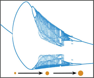
In figure 2, we show a typical evolution of an ensemble of particles in the position space. In figure 2(a), we have a uniformly seeded particle ensemble with $R=0.84$, $St=0.22$, each particle coloured either in maroon or black. Figure 2(b) shows their respective positions after 10 time periods of rotation: the maroon patch of particles has converged to an attractor (a limit cycle here) whereas the black patch of particles has centrifuged out spirally. Since we are interested in clustering and trapping behaviour of particles, centrifuging particles (coloured black in the figures) are excluded from our study and the results therein.

Figure 2. Typical evolution of an ensemble of inertial particles $(\rho _p/\rho _f>1)$ in the position space, in the rotating frame of an identical vortex pair. The particles are uniformly seeded near the vortex pair as shown in (a). Particles after 10 time periods of rotation, evolved under reduced MRE, are shown in (b). A fraction of particles (coloured maroon) get trapped to an attractor such as a fixed point or a limit cycle. However, a majority of particles (coloured black) are centrifuged out in spiralling orbits. The former set of particles forms our primary focus.

In the upcoming sections, we restrict our discussion to a co-rotating vortex pair of identical strengths, and to the case of particle velocity initialised to zero in the rotating frame. Unequal vortex strengths and different initial conditions are discussed in Appendices A and B, respectively. We see that while the behaviour is qualitatively similar, significant quantitative variations can exist. Thus, our model flow is to be treated as one bringing out general physical features of trapping and clustering, and not as a predictive tool.

3. Particle trapping dynamics

Region II in figure 1(b) is of special interest in the context of particle trapping. Attracting orbits of various descriptions are contained within this region, allowing trapping of particles for long times. Moreover, a high level of clustering happens in this region, which is of significance in different contexts. We discuss Region I no further, except to mention that inertial particles which begin within them are expected to display the standard centrifuging behaviour to leave the vicinity after a brief transient (Ravichandran & Govindarajan 2015).

The Stokes number $St$ and the density parameter $R$ are the pertinent non-dimensional numbers in our context. At the initial time, particles of a fixed $St$ and $R$ are placed in a dense uniform grid across a region of interest, and their asymptotic behaviour is categorised. Broadly, higher-Stokes-number particles quickly exit the region whereas those at lower Stokes number can either be trapped in the vicinity forever, or spend varying amounts of time in the vicinity before leaking out.

We begin by examining the dynamics in the absence of the BBH force. Under this approximation, we have a finite-dimensional nonlinear dynamical system, and standard principles for the behaviour of such systems apply. The case where $R=0.84$, i.e. each particle is $1.285$ times denser than the fluid, is discussed first since it displays what we term as canonical behaviour in this context, namely that the attractor undergoes successive period-doubling bifurcations to chaos. Typical attractors for particles of increasing Stokes number are shown in panels (i) of figure 3: a fixed point, a period-2 limit cycle and a chaotic (strange) attractor. We remark that these attractors as shown are in a rotating frame. What appears as a fixed point in figure 3(a) is actually a point which undergoes periodic motion along a circle in the laboratory-fixed frame. Thus, particles which collect here are in continuous motion. Similarly, what appears as a limit cycle in the rotating frame fills an annular region in the laboratory frame. All particles starting within the corresponding BoAs shown in panels (ii) of figure 3 asymptotically reach their respective attractors and never leave the vicinity.

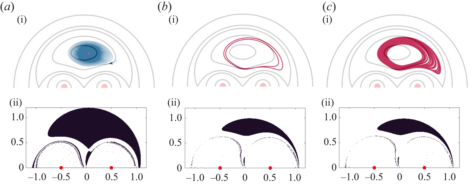
Figure 3. Typical asymptotic states shown in maroon (i) and their corresponding basins of attraction (ii) for a finitely dense inertial particle with density factor $R=0.84 \ {(\rho _p/\rho _f \approx 1.3)}$ and varying Stokes number $St$, without the BBH force: (a) $St=0.09$. (b) $St=0.22$. (c) $St=0.24$. Red dots indicate the vortex centres in the rotating frame. In (a) the particle spirals (shown in blue) into a fixed point attractor, whereas in (b,c) the particle is trapped into a limit cycle of period 2 and a strange attractor, respectively. The orbits are overlaid on the separatrices of the background flow for clarity of their scale and location. Mirror-symmetric patterns exist in the lower half-plane.

Next, we construct a bifurcation diagram, shown in figure 4 for $R=0.84 {(\rho _p/\rho _f \approx 1.3)}$. Below $St\approx 0.12$, the attractor is a fixed point, and beyond we have limit cycles of increasing complexity. The extrema on the horizontal axis of the limit cycles are plotted on the ordinate of the figure. A textbook period-doubling route to chaos ensues. We have checked that the Stokes number gap between successive bifurcations goes down asymptotically as the Feigenbaum number, with chaos setting in at $St=0.232$. It is seen that the BoA for the higher Stokes number is smaller (see figures 3 and 6).

Figure 4. Bifurcation diagram for $R=0.84 \ {(\rho _p/\rho _f \approx 1.3)}$ without the BBH force. An attracting fixed point exists below $St=0.12$, whereas for $0.12 < St < 0.22$ we have a period-1 limit cycle, followed by ever more complex limit cycles as the Stokes number increases. There are no asymptotic attractors beyond $St_{crit}=0.24675$.

A general observation which is relevant for all the attractors we find is as follows. The attractors are manifolds of dimension lower than two. This means all particles which initially occupy a 2-D BoA not only remain in the vicinity indefinitely, but actually converge on to objects of smaller dimension. This focusing of particles is a signature of caustics formation, and is indicative of extreme clustering. The clustering thus achieved can enormously enhance opportunities for collision and coalescence. Whether for carbonaceous material in the ocean participating in carbon fixing, swimmers who benefit from clustering in their quest for reproduction or dust in protoplanetary discs agglomerating into planetesimals, such attractors are thus of consequence.

The stage is now set to discuss the physics we miss when the BBH force is neglected, as well as to bring to light the non-monotonic and counterintuitive response of the system to both $St$ and $R$. Figure 5 shows the bifurcation diagram for $R=0.84 \ {(\rho _p/\rho _f \approx 1.3)}$ with the inclusion of the BBH force. Though the dynamics now is not a standard dynamical system in the position–velocity state space, we obtain fixed points and limit cycles. The contrast with figure 4 is self-evident. Interestingly, the bifurcation from a fixed point to a limit cycle occurs at a similar Stokes number with and without the BBH force. However, the period-1 limit cycle persists with the BBH force up to a rather large Stokes number of $St_{crit}\approx 0.5$ whereas without the BBH force, there was no attractor beyond $St \approx 0.25$. The fact that trapping of particles of relatively large inertia takes place in this simple vortical system is remarkable, and underlines the need for including the BBH force in our studies. As the Stokes number approaches the critical value, we find the BoA splitting into two with a very small BoA corresponding to a period-2 limit cycle (shown in green in figure 5), while the vast majority of particles are attracted to the period-1 cycle. As previously seen in panels (ii) of figure 3, the BoA is a sensitive function of the Stokes number.

Figure 5. Bifurcation diagram for $R=0.84 \ {(\rho _p/\rho _f \approx 1.3)}$ with the inclusion of the BBH force. Trapping prevails for a wider range of Stokes numbers than without the BBH force (compare with figure 4). A period-2 limit cycle (shown in green), with a very small BoA, coexists with the period-1 limit cycle (in orange) near $St_{crit}\approx 0.5$.

The area of the BoA is a direct measure of the fraction of particles which get trapped in an attractor. The area of such BoA is obtained for a range of Stokes numbers, and shown in figure 6, with and without the BBH force, for $R=0.84 {(\rho _p/\rho _f \approx 1.3)}$. The measurement involves storing the initial locations of all particles which get trapped in the attractor, and calculating the area of the region over which the initial locations are spread. Whether with or without the BBH force, as the Stokes number becomes higher, i.e. particles become more inertial, their propensity to leave the vicinity monotonically increases. Thus, the BoAs shrink steadily. At this value of $R$, this feature is as would be intuitively expected, but we shall soon see different behaviour for particles that are denser. There is a sharp cut-off at a Stokes number, which we refer to as $St_{crit}$, beyond which no particles are trapped. The $St_{crit}\approx 0.25$ for the case without the BBH force, and is significantly greater at $St_{crit}\approx 0.5$ when the BBH force is included. Close to $St_{crit}$, the BoA shows a sensitive dependence on Stokes number, i.e. a rapid shrinking of the area of the BoA to zero. The behaviour past the critical Stokes number is ‘leaky’, i.e. particles slowly escape from the region of interest. Notably, in addition to missing the significant trapping of particles of larger inertia, the fraction of particles trapped is seen to be grossly underestimated at all Stokes numbers by neglecting the BBH force. In the case with the BBH force the period-doubling route is left incomplete.

Figure 6. Variation of the area of the BoA with the Stokes number for $R=0.84 {(\rho _p/\rho _f \approx 1.3)}$, with and without the BBH force.

We move on to higher particle density, i.e. smaller $R$, with bifurcation plots shown in figure 7. Changing the density ratio introduces unexpected features in the dynamics. In figure 7(a,b) we see period-doubling bifurcations followed by unusual period-halving bifurcations back to a fixed point at higher Stokes number. We also see that a small difference in density ratio changes the behaviour from chaotic to periodic. For the same density ratio as in figure 7(a), the inclusion of the BBH force converts the dynamics to that on a canonical period-doubling bifurcation route to chaos, as seen in figure 7(d). Interestingly, at this density ratio too, the BBH force does not significantly change the Stokes number at the first bifurcation occurs: going from fixed point to limit cycle. Through most of the range of $St$, a fixed point or a limit cycle persists, followed by a rapid breakdown into chaos within a short range of Stokes number. At the larger density ratio of ${\sim }7$ (figure 7c), only two small regimes of particle trapping are seen. In contrast, with the inclusion of the BBH force, figure 7(d,e), trapping is more widespread across $St$. A period-halving bifurcation occurs here too (figure 7e), but at a higher density ratio than without the BBH force. Here too, at higher Stokes, we regain a fixed point as the sole attractor. Another non-standard feature seen in several of these bifurcation diagrams is the existence of gaps. Within these windows, no particles are trapped in the vicinity of the vortices. In fact, in figure 7(e), two windows are visible, so the actual Stokes number of the period-halving bifurcation, from a $2$-cycle to a simple limit cycle, is not obtainable, though a period-$1$ limit cycle followed by a fixed point are evident at higher Stokes numbers. In particulate flows, we have come to expect a monotonic trend in complexity as the Stokes number increases, so the transition, as we move up in $St$, from an attractor, to no particles being trapped, and back to particle-trapping in an attractor, is worthy of remark. Moreover, during period-halving, an increase in $St$ simplifies the attractor, and we hope that these findings alone will be intriguing enough to the reader to be motivated to explore particulate flows in this context.

Figure 7. Bifurcation diagrams for different representative density ratios: (a) $R\,{=}\,0.5\,{(\rho _p/\rho _f\,{=}\,2.5)}$; (b) $R\,{=}\,0.48$ ${(\rho _p/\rho _f \approx 2.6)}$; (c) $R=0.2 \ (\rho _p/\rho _f = 7)$; (d) $R=0.5 \ {(\rho _p/\rho _f = 2.5)}$; (e) $R=0.2 \ {(\rho _p/\rho _f = 7)}$. In (a–c) the BBH force is neglected, whereas in (d,e) it is included. On the ordinate are the extrema of the $x$-coordinate of the asymptotic trajectories.

With these examples, we demonstrate the general trend in our system: the long-time behaviour of inertial particles with the BBH force at a given density parameter $R$ is in broad qualitative agreement with the behaviour without BBH at a higher $R$. In other words, a denser particle, with the inclusion of the BBH force, behaves qualitatively like a lighter particle without the BBH force, asymptotically in time.

Two sample BoAs are shown without the BBH force in figure 8(a,b), to give a visual idea of how the BoA shrinks as we approach $St_{crit}$. The Stokes numbers chosen correspond to period-doubling and period-halving bifurcations, respectively. Over a range of $St$, the areas of the BoA are shown in figure 8(c), with and without the BBH force, for a higher density ratio than in figure 6. Again, with the BBH force, we see the trapping of particles of significantly higher $St$ than the dynamics we obtain by neglecting would suggest. Moreover, the BoA is significantly larger with the BBH force than without for the entire range of Stokes number. We may conclude that the neglect of the BBH force will seriously underestimate the number of particles trapped in the vicinity of vortices. Interestingly at this higher particle density, in the absence of the BBH force, the size of the BoA varies non-monotonically with Stokes number, and a small non-zero fraction of particles remains trapped even at high Stokes number. We do not have an explanation for this anomalous behaviour. The anomalous behaviour vanishes in this case upon the inclusion of the BBH force, showing a monotonic decrease of BoA size with Stokes number and a rapid decrease to zero just before $St_{crit}$. We hasten to note that the dynamics including the BBH force too showed such anomalous behaviour elsewhere, as evidenced by the gap in figure 7(e) in the region $0.16< St<0.25$ where size of BoA drops to zero. Thus, this particular feature is not merely a consequence of neglecting the BBH force. Since particles of higher Stokes number get centrifuged out of the vicinity of vortices faster, we would have expected a shrinking BoA with increasing particle inertia. This canonical expectation is belied over some ranges of density ratio.

Figure 8. (a,b) BoAs for $R=0.5 \ {(\rho _p/\rho _f = 2.5)}$ without the BBH force during period-doubling ($St=0.320$) and period-halving ($St=0.483$), respectively (see figure 7a). Note the difference in sizes. (c) Variation of the size of the BoA with Stokes number at $R=0.5$, with and without the BBH force.

It is relevant to mention that these broad findings on the effect of the BBH force are in contrast with those for the flow past a solid cylinder (Daitche & Tél 2011, 2014), where the inclusion of the BBH force reduces caustics as well as destroys attractors. Such reduction in clustering was also seen by Guseva, Feudel & Tél (2013) in convective cell flow. Similarly, Chong et al. (2013) studied finitely dense inertial particles in a viscous streaming flow created by an oscillating cylinder, wherein they concluded that the BBH force resists particle trapping. Evidently, the physics of the BBH force cannot be oversimplified thus.

The case of the infinitely dense particle was studied by Angilella (2010) upon neglecting the BBH force, where it was shown analytically that there is a fixed point up to $St=(2-\sqrt {3})/2{\rm \pi}$ and no attractor beyond. We repeated the calculations with the BBH force included for $\rho _p\gg \rho _f$, and found the critical Stokes number unchanged. Further, our computations for the location of the fixed point for all Stokes numbers below this are in excellent agreement with the analytical results of Angilella (2010). We note the qualitative difference between infinitely dense particles and our largest density ratio of $R=0.2 (\rho _p/\rho _f=7)$ (figure 7e). We thus confirm that the BBH force has a noticeable effect on finitely dense particles, especially when particle densities are of the same order of magnitude as that of the surrounding fluid. This indicates that the BBH force should be included as a significant force when studying solid–liquid systems such as microplastics in the ocean.

To give an idea of the complexity in the solutions, we provide a phase plot in figure 9, where the behaviour across density ratios and Stokes number without the BBH force is summarised. Figure 9(a) shows the different kinds of attracting orbits that one obtains. At a given density ratio, as we move up in Stokes number, in some part of the regime, we go from attracting orbits to no attracting orbits, whereas in other portions we can go back to attracting fixed points or limit cycles over a range of Stokes numbers. We may identify the following three regimes: for $1 > R \gtrsim 0.5$ we have a period-doubling route to chaos, for $0.5 > R > 0.35$ a period-doubling route, which may go all the way to chaos or may be limited to a few bifurcations, is followed by period halving, leading to a single fixed point, and for $0.35>R$ we have only attracting fixed point in the regime where we have trapped particles. With the BBH force, we have the three regimes, but the transitions all happen at lower values of $R$. In figure 9(a) the density ratio of $R \sim 0.5$ is most interesting, where the existence of attracting orbits at large Stokes number is possible, and there is sensitive dependence on the density ratio. Chaotic attractors only exist at $R\gtrsim 0.5$, i.e. when the particle and fluid densities are comparable. Here, too, the range of Stokes numbers at a given $R$ over which chaotic attractors are seen is very narrow. The corresponding areas of the BoA are shown as a phase plot in figure 9(b). Broadly, at low Stokes numbers, as the particles become denser, the BoA shrinks. However, at intermediate Stokes number and density ratios, we see non-monotonic behaviour. As $R \to 1$ (i.e. $\rho _p \sim \rho _f$), the particles are near neutrally buoyant, and over a range of Stokes numbers, the entire region II corresponds closely to the BoA. Invariably, in this limit, the attractor is a fixed point.

Figure 9. Phase plots for inertial particles, without the BBH force, based on (a) the period of the attracting orbit. The regime occupied by limit cycles of period 2 and above is very narrow. (b) The logarithm of the size of the BoA. Particles of near-neutral densities tend to stay longer. In both plots, there is anomalous behaviour at $R \sim 0.5$.

4. Particle leakage

We have seen that for every density ratio $R$, there is a critical Stokes number, $St_{crit}$, above which no particle remains indefinitely in the vicinity of the system. We now ask what happens beyond $St_{crit}$. Figure 10 shows two sets of particle trajectories, with the same initial conditions, but one with $St$ slightly less than $St_{crit}$ and the other with $St$ slightly greater than $St_{crit}$. The first set is trapped forever, whereas the second set escapes. At $St=St_{crit}$ one point on the chaotic attractor in phase space coincides with the saddle point. This is termed a crisis, (Grebogi, Ott & Yorke 1983), where the chaotic attractor disappears, making way for a chaotic saddle. The dynamics near the chaotic saddle is ‘leaky’, i.e. all particles near the chaotic saddle will leave the vicinity in finite time.

Figure 10. Leakage of particles past the trapping criteria without the BBH force, for the representative case of $R=0.84 \ {(\rho _p/\rho _f \approx 1.3)}$ with $St_{crit}=0.24675$. The trajectories of a set of particles in the narrow range $St\in (0.2465,0.2470)$ about $St_{crit}$, with identical initial conditions, are shown. Trajectories for $St < St_{crit}$ are coloured red, where particles are seen to remain trapped, whereas those for $St > St_{crit}$ are coloured blue, where particles escape. The green dot is the saddle fixed point at $St_{crit}$, whose location does not vary visibly for the narrow range of $St$ shown.

A particle starting at a given location is traced until it leaves the system, and the time at which it leaves the system is noted down as its residence time within the region of interest. We define the ‘system’ by a circle of radius $2$, centred at the origin. While the numbers for residence time depend weakly on this choice, a change in the definition will not change our conclusions. This residence time is plotted for all initial locations in figure 11, for three Stokes numbers. At $St=0.24$, which is less than $St_{crit}$ (figure 11a), we have a patch of particles whose residence time is nominally equal to the simulation time $T_{max}$, and we have confirmed that this patch corresponds to the BoA whose particles are permanent residents. However, past the critical Stokes number, at $St=0.25$, all particles escape at finite times (figure 11b). There are sharp ridges in the figure, and particles originating on these have a large residence time. These ridges are separated by valleys of very low particle residence times. Although the area of the BoA is zero, the fact that particles can remain in the vicinity and close to each other for tens of rotation time-scales signifies the enhanced opportunity for collisions even beyond $St_{crit}$. At the even higher $St$ of $0.255$, in figure 11(c), the residence times have already dropped significantly.

Figure 11. Residence times of inertial particles for the density ratio $R=0.84 \ {(\rho _p/\rho _f \approx 1.3)}$, without the BBH force: (a) $St=0.24\ {< St_{crit}}$; (b) $St=0.25\ {> St_{crit}}$; (c) $St=0.255\ {> St_{crit}}$. The colour at a given position indicates the residence time of a particle starting at that location.

The stable manifold of the saddle point corresponding to the case in figure 11(b), at $St=0.25$, is shown in figure 12(a) for $v_0=0$ particles. It theoretically represents the original locations (in phase space) of particles which flow into the saddle, approaching it as $t\to \infty$. It occupies zero area and has a fractal dimension of approximately $1.7$. A particle starting exactly on the stable manifold would have infinite residence time. Particles starting very close to the stable manifold will have large but finite residence times. Therefore, we see a close correspondence between the ridges of high residence times in figure 11(b) and the stable manifold in figure 12(a). The fractal nature of the stable manifold and the fractal distribution of ridges and valleys in the residence time plot are signatures of transient chaos (Tél 2015). In figure 12(b), we show that the fractal dimension of the stable manifold falls sharply as $St$ increases. A stable manifold of fractal dimension $1$ indicates no transient chaos, and the reduction in fractal dimension with increasing Stokes indicates a corresponding reduction in transient chaos.

Figure 12. (a) Stable manifold of the saddle point shown by the blue dot (slightly shifted for clarity), for $R=0.84 \ (\rho _p/\rho _f \approx 1.3)$ and $St=0.25$, without the BBH force. The manifold shown is a fractal object with an approximate fractal dimension of $1.7$. The vortex centres are indicated by red dots. (b) Fractal dimension, calculated using the box-counting method, for $St>St_{crit}$ for $R=0.84\ (\rho _p/\rho _f\approx 1.3)$. Error bars indicate the variation in the calculated dimension for different box sizes. The dotted line indicates the trend and is not an exact quantitative measure.

In figure 13(a,b), we plot the residence times including the BBH force at $R=0.84 \ (\rho _p/\rho _f \approx 1.3)$, just below and above the $St_{crit}{\approx 0.5}$. As before, when $St< St_{crit}$, the residence time for particles in the BoA, denoted by the dark patch in figure 13(a), is infinite. We recall from figure 5 that the corresponding attractors are the coexisting simple period-1 limit cycle and a period-2 limit cycle, with the latter associated to a very small BoA. In the case without the BBH force, we had seen that the residence times outside the BoA were very small, but here, we find long residence times in the valleys as well. These valleys spiral inward as we increase $St$ where the BoA shrinks rapidly (as was seen in figure 6). Just beyond $St_{crit}$ the residence time plot is given by figure 13(b). Again we find closely spaced ridges and valleys in the residence times. In contrast to the case without the BBH force, where we found a chaotic saddle with long-lasting transients close by, here we do not find any evidence of a chaotic saddle. Instead, a significant number of particles spend a long time near a structure which resembles period-1 orbit before eventually escaping. Although with the BBH force, we no longer have a standard dynamical system in the position–velocity state space, this structure resembles a periodic-orbit saddle seen in standard dynamical systems.

Figure 13. Residence time plots with the inclusion of the BBH force for two density ratios around their corresponding critical Stokes numbers: $R=0.84\ {(\rho _p/\rho _f \approx 1.3)}$ with $St_{crit}\approx 0.5$ in the top panels (a,b) and $R=0.50 \ {(\rho _p/\rho _f = 2.5)}$ with $St_{crit}\approx 0.69$ in the bottom panels (c,d). For each $R$, a plot each is provided for a $St$ slightly below and slightly above the respective $St_{crit}$: (a) $R=0.84,\ St=0.495< St_{crit}$; (b) $R=0.84, St=0.508>St_{crit}$; (c) $R=0.50,\ St=0.685< St_{crit}$; (d) $R=0.50,\ St=0.705>St_{crit}$.

In figure 13(c,d), the residence time is provided for $R=0.5$, just below and just above $St_{crit}$, respectively. The BBH force is included. It will be recalled from figure 7(d) that there is a chaotic attractor before the sudden disappearance of the BoA. This is reminiscent of $R=0.84$ without the BBH force. The irregular spatial distribution of residence times in figure 13(d) is also similar to the plots in figure 11(b,c). All these are signatures of transient chaos.

For both $R=0.5$ and $R=0.84$, at $St$ just below $St_{crit}$ the basin boundary itself has an irregular fractal-like structure, which was absent without the BBH force. We note that fractal basin boundaries arise in the context of inertial particles in flow, such as, for heavy ($R=0$) inertial particles due to the interplay between transient chaos and fixed point attractors (Angilella et al. 2014), and for finitely dense inertial particles due to the addition of the BBH force (Guseva et al. 2013).

We see that residence times can vary greatly, even for particles starting out at neighbouring locations. It is thus worthwhile to calculate the probability densities of residence times. Figure 14(a) shows the distribution of residence times, without the BBH force, for all particles initialised in the region of interest for four Stokes numbers above the critical. The distributions are all exponential, which is a signature of transient chaos, i.e. the existence of a chaotic saddle (Tél 2015). Note that even beyond $St_{crit}$ the residence times are still $O(10)$ time periods, which can be significant. However, note that residence time does decrease very rapidly as we move away from $St_{crit}$. Figure 14(b) is a corresponding residence time distribution plot for the same density ratio, but with BBH, for particles whose Stokes number is just above the critical. While the long residence time particles display a short exponential-like feature, over moderate residence times, we see that the probability of a given residence time varies non-monotonically with the residence time. This is another feature we obtained only with the inclusion of the BBH force, which means further study is needed to understand the nature of the transients beyond $St_{crit}$ with the BBH force.

Figure 14. Distributions of residence times of inertial particles of $R=0.84$, at Stokes numbers just beyond the critical, as indicated in the legends. (a) In the absence of the BBH force, we see an exponential distribution of residence times. The slope increases rapidly as $St$ moves further away from $St_{crit}\ (=0.24675)$. (b) In the presence of the BBH force. Particles which last a long time in the vicinity display an exponential distribution in residence times, whereas the probability of staying is non-monotonic in the residence time at smaller residence times. Here $St_{crit} \approx 0.5$.

The regions in the $R$–$St$ parameter space where a significant number of particles have a large but finite residence time are shown in figure 15, without the BBH force. We note the non-monotonicity in Stokes number here too. Close to neutral density, long-lasting transient are seen to be extensive, and can be an important contributor to particle collisions. Away from neutral density ($R=1$), most of the particles which eventually escape do so within a few time periods ($O(T)$), so the phenomenon of trapping and clustering becomes evident early on. However, to visual accuracy, the convergence time of trapped particles to their respective attractors can be $O(10 T)$, or even higher with the BBH force.

Figure 15. Logarithm of the size of basins occupied by particles with long but finite residence time, i.e. $T_{esc}>10T$. Note that as $R \to 1$, i.e. the particle becomes more neutrally buoyant, a significant fraction of particles can have long residence times for a significant range of $St$.

5. Summary and discussion

We have examined the dynamics of inertial particles that are denser than the fluid in the simplest rotating and vortical system: that of two identical vortices in periodic circular motion. We have found significant levels of particle trapping in the vicinity, even for particles of significant Stokes number. The inclusion of the BBH force results in higher levels of trapping for a given Stokes number, i.e. much larger BoA. It also results in a wider range of Stokes number over which trapping occurs. These are in contrast to earlier findings on the effects of BBH in other flows. The trapped particles are attracted to fixed points or limit cycles of varying complexity, all the way to chaotic attractors. Thus, there is extreme clustering into lower-dimensional (zero area) manifolds, of particles initially in a finite BoA. Particles in a rotating system thus do not follow the expectation that they will constantly centrifuge out of vortical regions, and collect in regions of high strain. In fact, the attractors do not correspond to the highest strain regions.

The trapped particles undergo a rich variety of dynamics in the $R$–$St$ parameter space. The BoA is in some part non-monotonic function of the Stokes number and, in fact, we can have a range of Stokes numbers devoid of particle-trapping. A period-doubling route to chaos is observed in some parameter ranges, whereas an unusual period-halving back to a fixed point is seen in other parts of the parameter space. This regime is physically interesting because it belies the expectation gained so far that particles of higher inertia have a propensity to attain more complicated limiting trajectories. A given behaviour observed at a given particle density without the BBH force appears at a much higher particle density (lower $R$) with the inclusion of the BBH force. Moreover, a given bifurcation typically happens at a higher $St$ with the BBH force than without.

Close to a critical Stokes number $St_{crit}$, which depends on $R$, there is a sudden drop in the BoA. Beyond this, no particles are trapped forever, since a crisis occurs and the chaotic attractor becomes a chaotic saddle. Beyond this, the system displays alternating ridges of high but finite residence time and valleys of low residence time. The range of Stokes number over which long-lasting transients are seen expands at particle densities close to neutral buoyancy. One remarkable qualitative difference with the addition of the BBH force is that the period doubling route to chaos can remain incomplete until the rapid disappearance of the attractor. Correspondingly, the transient dynamics beyond $St_{crit}$ resemble the dynamics near a non-chaotic saddle. Further, the distribution of residence times is exponential without the BBH force and also with the BBH force for higher values, but is non-monotonic with the BBH force just beyond $St_{crit}$. Just before the crisis, the basin boundaries with the BBH force appear to have a fractal nature, unlike without the BBH force. Thus, the case with the BBH force merits further inquiry in this context.

We now discuss the limitations of our model. We recall that the MRE is a model equation derived in the small particle Reynolds number limit, $Re_p \rightarrow 0$. In practical scenarios where $Re_p$ is only finitely small, the effects due to flow inertia will become significant in long but finite time. Therefore, the validity of the MRE in various regards including the form of the history force and quasi-steady drag force are questionable after long simulation time. However, our results are valid and insightful in the cases where significant clustering is observed within short times, subject to the condition $Re_p<1$.

The MRE is widely used at Stokes numbers of $O(1)$ but the need to satisfy this requirement simultaneously with $Re_p \ll 1$, as well as keeping the particle size small, i.e. $a/d \ll 1$ imposes additional restrictions. By expressing $Re_p$ in terms of our control parameters $R$ and $St$, we obtain the scaling relation $Re_p (a/d) \sim R St |v_{rel}|$, where we recall that $v_{rel}$ is a non-dimensional quantity. For a small particle under the influence of a single vortex, the vortex turnover time may be used to define $St$. In our model, the $St$ is defined using the system's period of rotation. In both cases, when $St \sim O(1)$ we usually have $|v_{rel}| \sim O(1)$. In principle, the above scaling requirement can be satisfied if $R \to 0$, but in an experiment, even in the extreme limit of solid particles in air, we typically have $R \sim 10^{-3}$ at the lowest. Demanding arbitrary smallness of the particle size $(a/d)$ is therefore penalised by large $Re_p$ near vortices. For finite density ratios, as in our case, satisfying the requirements is even harder. From our computations of slip velocity, we find that the slip velocities with the BBH force are usually significantly lower than without it. At the highest Stokes numbers in our study, $Re_p \sim O(10)$ for $a/d \sim O(10^{-2})$ for some part of the dynamics. However, close to the fixed points, and often near the limit cycles, slip velocities are low and so is $Re_p$. The small $Re_p$ assumption is more reasonable for very dense and near-neutrally buoyant particles. Due to this, and the findings in Maxey, Chang & Wang (1996) that show applicability of the MRE for $Re_p \lesssim 17$, we expect that our findings have qualitative significance. In fact, the MRE (with the BBH force) has been previously used to study chaotic dynamics for $Re_p\sim O(1)$ (Daitche & Tél 2014; Daitche 2015) in a different flow. We note that estimates of $Re_p$ are rarely discussed in the literature, and need more attention. There is a need for modelling unsteadiness at higher Reynolds numbers for different background flows. For higher particle concentrations a stochastic model based on particle resolved simulations has been provided (Tavanashad et al. 2019; Lattanzi et al. 2022) where inter-particle interactions, and their history effects, have been accounted for.

Our model also assumes one-way coupling between the particles and the underlying fluid and therefore our results hold in the dilute limit of particle concentration. If the concentration of particles becomes high due to clustering itself, the feedback of particles on the fluid is no longer negligible. Feedback from particles is known to affect vortex merger (Shuai, Roy & Kasbaoui 2024). In these cases a separate study on inertial particles in the ensuing flow dynamics under two-way coupling is required. We have ignored gravity from our model to isolate and study the effects of hydrodynamic forces on inertial particle dynamics. Although co-rotating vortices do occur commonly in turbulence, the merger process will include effects from the rest of the flow, as well as viscous effects depending on the local flow Reynolds number. The relevance of our results for true turbulence will therefore be affected by these other factors.

In spite of its limitations, our toy model study brings to attention an important aspect of extreme clustering in rotating flows. In fact if the rotation rate is externally applied rather than driven by a flow, we get an extra handle which can potentially mitigate the limitations. The attraction of particles towards a manifold of dimension smaller than the spatial dimension, like a pair of fixed points or limit cycles, will result in extreme clustering. This can be a major contributor to particle collision and agglomeration, and in the case of tiny living organisms, to enabling communication and sexual reproduction. The relevance of these findings to particle aggregation in protoplanetary discs, in rotating systems in the ocean and also in turbulent-flow neighbourhoods dominated by a few strong vortices are worth investigation. Future studies on simple model flows, consisting of characteristic combinations of vortices, with and without rotation of the entire system, in two and three dimensions, would be illuminating, and provide a platform to understand some features of particulate turbulent flows. We therefore hope that our work will motivate experiments and further theory on this important question.