The transition from re-entrant flow-driven to shockwave-driven cloud cavitation

Abstract

Understanding the mechanism of hydrodynamic cloud cavitation is crucial to reducing noise, vibration and wear. Recent studies have clarified the physics of two distinct formation mechanisms of cloud cavitation. Ganesh et al. (J. Fluid Mech., vol. 802, 2016, pp. 37–78) identified the propagation of bubbly shockwaves as a cloud detachment mechanism. Pelz et al. (J. Fluid Mech., vol. 817, 2017, pp. 439–454) explained the influence of Reynolds number and cavitation number on asymptotic growth of the cavity sheet and its periodic shedding caused by re-entrant flow. In this paper the two mechanisms are set in relation to each other. For this, we show firstly that the transition from re-entrant flow to shockwave-driven cloud cavitation is given by a kinematic condition, namely the asymptotic sheet length equates to the chord length, $\hat {a}=L$. For $\hat {a}>L$ shockwave-driven cloud cavitation dominates. For $\hat {a}< L$ re-entrant flow-driven cloud cavitation dominates. As the cavitation number decreases, the closure region of the cavity sheet reaches the trailing edge of the hydrofoil, identifying the trailing edge as a trigger for condensation shockwaves, particularly as re-entrant flow-driven cavitation diminishes. Since the sheet length is an implicit function of the cavitation number, the kinematic condition $\hat {a}/L=1$ results in a critical cavitation number ${\sigma _\mathrm {II,III}}$ that is calculated analytically and validated by experiments. Secondly, we derive the relationship between the Strouhal number and the asymptotic sheet length for re-entrant flow-driven cloud cavitation. The model presented here is thoroughly validated by experiments.

1. Introduction

Cloud cavitation is among the most severe manifestations of cavitation, specifically concerning its potential to cause damage. It refers to the periodic detachment and advection of large-scale cavitation vortices, observed in pumps, ship propellers, nozzles, etc. associated with unsteadiness leading to noise and potentially to vibration, efficiency drop and erosion.

Cloud cavitation has four phases: (i) nucleation near the leading edge of the hydrofoil, (ii) asymptotic sheet growth to a sheet length $\hat {a}$, (iii) detachment of cavitation clouds, i.e. bubbly vortices, and advection due to the bulk flow, and (iv) cloud collapse.

Over many years, the re-entrant flow – a thin and viscous liquid film flow developing at the cavity closure region, which flows beneath the cavity sheet – was believed to be the sole mechanism driving cloud cavitation: Knapp (1955) firstly reported periodic cloud cavitation due to the re-entrant flow, followed by many notable studies (Furness & Hutton 1975; Lush & Skipp 1986; Le, Franc & Michel 1993; De Lange & De Bruin 1998; Pham, Larrarte & Fruman 1999; De Graaf, Brandner & Pearce 2017; Pelz, Keil & Groß 2017; Smith et al. 2020). Kawanami et al. (1997) demonstrated in their experiments on the flow around a hydrofoil the existence of the re-entrant flow using dye injections as well as an obstacle to hinder the re-entrant flow reaching the leading edge, suppressing cloud cavitation. Callenaere et al. (2001) reported that the development of the re-entrant flow depends on the adverse pressure gradient and the thickness relation between the cavity and the re-entrant flow. Re-entrant flow-driven cloud cavitation occurs when the re-entrant flow reaches the cavity leading edge and breaks through the cavity sheet. The fundamental cloud shedding frequency associated with the re-entrant flow is known to decrease with decreasing cavitation number for otherwise constant flow conditions (Arndt et al. 2000; Kjeldsen, Arndt & Effertz 2000; Dular & Bachert 2009; Smith et al. 2020; Hatzissawidis, Ludwig & Pelz 2021). This happens because the asymptotic sheet length becomes larger; as a result, the sheet takes more time to develop, and the re-entrant flow needs to travel a longer distance. The asymptotic sheet length, as introduced by Pelz et al. (2017), refers to the theoretical sheet length that would be reached over infinite time, i.e. as $t \rightarrow \infty, a(t) \rightarrow \hat {a}$.

Apart from the re-entrant flow, there is a second mechanism for cloud cavitation at low cavitation number, namely the propagation of shockwaves. Shockwaves in bubbly flows are associated with a severe drop in the speed of sound of a liquid–gas bubbly mixture. Reisman, Wang & Brennen (1998) laid the groundwork for recognising the critical role of shockwaves in cloud cavitation, although they had been posited decades earlier by Jakobsen (1964).

Ganesh, Makiharju & Ceccio (2016) firstly described in detail shockwave-driven cloud cavitation in a nozzle with a wedge geometry using X-ray densitometry and high-speed visualisation. They associated the transition from re-entrant flow-driven cavitation to shockwave-driven cavitation with a critical Mach number. This investigation initiated experimental (Wu, Maheux & Chahine 2017; Jahangir, Hogendoorn & Poelma 2018; Wu, Ganesh & Ceccio 2019) as well as numerical studies (Budich, Schmidt & Adams 2018; Trummler, Schmidt & Adams 2020) regarding shockwaves in cloud cavitation.

The transition between the two regimes, which manifests as an abrupt change in the dynamics between a high-frequency and low-frequency shedding, was identified by Arndt et al. (2000) and Kjeldsen et al. (2000) for the flow around a NACA 0015 hydrofoil, and has also been reported by Leroux, Coutier-Delgosha & Astolfi (2005) and recently by Jahangir et al. (2018), Smith et al. (2020) and Bhatt, Ganesh & Ceccio (2023). The high-frequency shedding was associated with the re-entrant flow, the low-frequency with shockwaves, as first reported by Arndt et al. (2000).

Recent and insightful experimental studies about a NACA 0015 hydrofoil conducted by Bhatt et al. (2023) are consistent with the findings in this study. They have revealed a smooth transition, wherein re-entrant flow and shockwaves manifest with a specific probability expressed as a likelihood function over the cavitation number. At lower cavitation numbers, there is an increased probability of the occurrence of shockwaves.

Despite recent experimental and numerical activities, there is still a lack of knowledge regarding the transition from re-entrant flow-driven cavitation to shockwave-driven cavitation. The primary question addressed in the current study is: What is the condition that causes the transition from shockwave-driven to re-entrant flow-driven cloud cavitation for lifting surfaces? Our hypothesis is that the transition occurs if $\hat {a}=L$, i.e. when the closure region of the cavity sheet hits the hydrofoil's trailing edge of chord length $L$.

To address this question and to validate the hypothesis, we first draw a rough picture in § 2 for the transition mechanisms and dynamics about a hydrofoil. By using the condition $\hat {a}/L=1$, we identify a critical cavitation number, where the transition from re-entrant flow-driven cloud cavitation to shockwave-driven cloud cavitation occurs, § 2.1. We further predict the Strouhal number for the re-entrant flow-driven cloud cavitation from the sheet velocity and re-entrant flow dynamics described by a second-order nonlinear ordinary differential equation in § 2.2. After deriving the physical models, we introduce the experimental set-up in § 3 and conduct an experimental validation in § 4. The conclusions are summarised in § 5.

2. Cloud cavitation dynamics and physical modelling

A schematic representation delineating the mechanisms of shedding and transition is illustrated in figure 1. The transition from sheet cavitation, regime I, to re-entrant flow-driven cloud cavitation, regime II, is examined by Pelz et al. (2017). The present study deals with the transition from regime II to shockwave-driven cloud cavitation, regime III.

Figure 1. Schematic overview of the three cloud shedding mechanisms: I sheet cavitation, II re-entrant flow driven and III shockwave driven.

In this study, we consider the flow about a hydrofoil. The velocity and static pressure at infinity are denoted by ${U_\infty }$ and ${p_\infty }$, respectively. The operation point is given by the cavitation number, $\sigma := 2\,({p_\infty }-p_{v})/\varrho U_\infty^2$, where $p_{v}$ is the vapour pressure and $\varrho$ is the density of water, and the Reynolds number, $Re := {U_\infty } {L_{0}} / \nu$, where $\nu$ is the kinematic viscosity of water. The shape of the hydrofoil, i.e. NACA 0015 and the incidence $\alpha$, give the pressure distribution along the suction side for the non-cavitating hydrofoil ${c_{p}(x/{L_{0}}):= 2(\,p(x/{L_{0}})-{p_\infty })/\varrho U_\infty^2}$ with $p(x/{L_{0}})$ being the static pressure along the hydrofoil's surface. We distinguish between the nominal ${L_{0}}$ and the real chord length $L, L<{L_{0}}$, due to manufacturing reasons regarding the trailing edge as usual, cf. figure 1. We experience the different cavitation regimes as the static pressure ${p_\infty }$ and hence the cavitation number $\sigma$ at constant Reynolds number is reduced. At high cavitation numbers, a cavitation sheet is formed. This sheet is attached to a line near the leading edge, and is quasi-steady in the time average. It initiates as microscopic patches close to the leading edge and evolves into a macroscopic sheet, where small-scale horseshoe vortices are shed due to interfacial instabilities, cf. Brandner et al. (2010). This regime I is known as sheet cavitation. A further reduction of the cavitation number, leading to the surpassing of the critical value ${\sigma _\mathrm {I,II}}$, results in a well-defined periodic cloud shedding. This regime II is known as re-entrant flow-driven cloud cavitation with $\hat {a}<{L_{0}}$. Pelz et al. (2017) showed that ${\sigma _\mathrm {I,II}}$ is a function of Reynolds number and surface roughness.

From the point of view of dimensional analysis, the asymptotic sheet length $\hat {a}$ is a function of the cavitation number $\sigma$, the dimensionless nucleation rate ${f_{0}} R_0/{U_0}$ ($\,{f_{0}}, R_0$ and ${U_0}$ are the nucleation rate, the initial bubble size at the cavity leading edge and the fluid velocity at the cavity interface, ${U_0} = {U_\infty } \sqrt {1+\sigma }$, respectively), and the shape that encompasses all dimensionless length scales of the body, i.e. $\mathrm {shape}=\{\alpha, \mathrm {NACA 0015}\}$, fully considered by $c_{p}(x/{L_{0}})$. Hence, the dimensional analysis yields $\hat {a}/{L_{0}}=\mathrm {fn}(\sigma, {f_{0}} R_0/{U_0}, \mathrm {shape})$ or implicitly $0=\mathrm {Fn}(\sigma, {f_{0}} R_0/{U_0}, c_{p}(\hat {a}/{L_{0}}))$. The abbreviations $\mathrm {fn}$ and $\mathrm {Fn}$ are arbitrary explicit and implicit functions, respectively. Aligning with this, Pelz et al. (2017) derived the implicit expression of the asymptotic sheet length as

(2.1)\begin{equation} c_{p}(\hat{a}/L) \approx 1.67 \left(\frac{{f_{0}} R_0}{{U_0}}\right)^2 - \sigma. \end{equation}

This simple model is not only valid for a nozzle but also for flow about lifting surfaces such as the NACA 0015 hydrofoil, as the comparison with the experimental data in this work shows, cf. figure 2(b). As this paper further shows, the model also provides access to the critical cavitation number, which characterises the transition from regime II to III, cf. § 2.1.

Figure 2. (a) Welch spectrogram of the hydrophone signal; (b) experimentally determined sheet length compared with the analytical model from (2.1); (c) Strouhal number vs cavitation number for the shockwave-driven and re-entrant flow-driven cloud cavitation. The dashed vertical lines represent the critical cavitation numbers ${\sigma _\mathrm {II,III}}$ and ${\sigma _\mathrm {I,II}}$. The solid line is given by (2.3) with $C = {0.42}$ experimentally determined. (d) Sheet growth velocity. The Jupyter notebook for producing the figure can be found at https://www.cambridge.org/S0022112024012242/JFM-Notebooks/files/figure_2/figure_2.ipynb.

The large kinematic scales in regime II are the cloud shedding frequency $f$, and the sheet length $\hat {a}$. Assuming that the frequency $f$ is an explicit function of the dependent variable $\hat {a}$ and only implicitly dependent on the independent variables $\sigma, {f_{0}} R_0/{U_0}$ and ${U_\infty }$, as well as the shape of the hydrofoil, we obtain ${St:=f {L_{0}}/{U_\infty }=\mathrm {fn}({L_{0}}/\hat {a}, \mathrm {shape})}$. The first term of a Taylor expansion of this relation yields ${St\approx {L_{0}}/\hat {a} C(\mathrm {shape})}$, where $C$ is only a function of the body's shape. In fact this relation has been well validated by our experiments, see figure 2(a,c), and those of others, cf. § 1.

Regime III or shockwave-driven cloud cavitation occurs when the cavitation number $\sigma$ is lowered further: the sheet reaches the trailing edge, $\hat {a}/L=1$, and a shockwave is initiated, figure 1. It should be mentioned that in regime III a re-entrant flow may also contribute to a premature cloud shedding, although the main shedding cycle is driven by a shockwave (Budich et al. 2018; Venning, Pearce & Brandner 2022; Zhang et al. 2022). Furthermore, an advecting cloud from the previous cycle may influence the sheet growth or initiate a shockwave leading to an extinction of the growing cavity sheet, cf. Bhatt et al. (2023). However, the primary mechanism for the transition from regime II to III is attributed to the kinematic condition mentioned above, supported by the physical model and the experimental validation below.

Until now, shockwave-driven cloud cavitation, regime III, was described to be triggered by an abrupt stagnation in cavity growth. Ganesh (2015) came to this conclusion by the analysis of a nozzle flow which is not characterised by such a distinct typical length as is the case for the NACA 0015 hydrofoil with chord length $L$ used in this study. Budich et al. (2018) carried out a numerical study for the same set-up and associate the initiation of the shock with the adverse pressure gradient. However, in the present study, there is a clear kinematic condition $\hat {a}=L$ for the named transition. This hypothesis, in fact, is confirmed by the experimental model validation presented in this paper. The model is derived by predicting the sheet length $\hat {a}$ from which the critical cavitation number, ${\sigma _\mathrm {II,III}}$, is determined.

2.1. Critical cavitation number ${\sigma _\mathrm {II,III}}$

The critical cavitation number ${\sigma _\mathrm {II,III}}$ defines the transition from re-entrant flow-driven cavitation (II) to shockwave-driven cavitation (III) for a lifting surface. When the condition $\hat {a}=L$ is met, there is an abrupt stagnation of sheet growth, triggering a shockwave, and leading to a full extinction of the cavity sheet. From the asymptotic sheet length from (2.1), and the condition $\hat {a}=L$, the critical cavitation number ${\sigma _\mathrm {II,III}}$ yields

(2.2a,b)\begin{align} c_{p}\left(\frac{\hat{a}}{{L_{0}}}=\frac{L}{{L_{0}}}\right) = 1.67 \left(\frac{{f_{0}} R_0}{{U_0}}\right)^2 - {\sigma_\mathrm{II,III}} \quad \mbox{or} \quad {\sigma_\mathrm{II,III}} = c_{p}\left(\frac{L}{{L_{0}}}\right) - 1.67 \left(\frac{{f_{0}} R_0}{{U_0}}\right)^2. \end{align}

Due to the Kutta condition, there is a stagnation point in irrotational flow at the trailing edge, i.e. $c_{p}(1)=1$. However, from $L/{L_{0}} < 1$, the discontinuous trailing edge and viscous calculation (Drela 1989) follows $c_{p}(L/{L_{0}})\neq 1$.

The order of magnitude of the non-dimensionalised nucleation rate is $(\,{f_{0}} R_0/{U_0})^2 \sim 1$, taking into account values for the nucleation rate, ${f_{0}} \sim 10^5\ \mathrm {Hz}$, the initial bubble radius, $R_0 \sim 100\ \mathrm {\mu }\mathrm {m}$, and a typical velocity of ${U_0}\sim 10\ \mathrm {m}\ \mathrm {s}^{-1}$. These values align with the numerical study conducted by Hsiao, Ma & Chahine (2017) and the experimental study by Pelz et al. (2017) and Groß & Pelz (2017).

Groß & Pelz (2017) conducted a study on diffusion-driven nucleation in a generic test rig, operating at high cavitation numbers. They deduced and validated that the nucleation frequency is proportional to the supersaturation of the liquid, gas solubility and the Weber and Péclet numbers to the powers of $3/4$ and $1/3$, respectively.

In the present study, alongside diffusion, evaporation also plays a role. A nucleation rate and an initial bubble size cannot be derived from experiments, since the physics of the nucleation mechanism at the cavity leading edge are considerably more complex, particularly for hydraulically smooth surfaces where instabilities, such as spanwise-moving cells, develop in the separated boundary layer, cf. Brandner et al. (2010) and Venning et al. (2022).

van Rijsbergen (2016) offers a thorough overview of potential nucleation mechanisms near the leading edge. In our study, we focus on the inception of surface-bound nuclei at high incidence angles. We conceptualise the nucleation mechanism as parallel streaks, initiating near the leading edge, although we recognise that the underlying physics are more complex, involving boundary layer effects and hydrodynamic instabilities, as detailed by Brandner et al. (2010). The dimensionless nucleation rate used here can be interpreted as a rate of vapour and air production. Despite being a coarse and simple model, the predicted sheet length shows good agreement with the results, as discussed in the context of external flows in this study and internal flows in the study by Pelz et al. (2017).

2.2. Strouhal number

In the following we derive an analytical model for the constant $C$ being only dependent on the shape of the body; $C$ is also known as the Strouhal number based on the asymptotic sheet length and has been experimentally found to be within $1/4$ to $2/5$ (Kawanami et al. 1997; Pham et al. 1999; Callenaere et al. 2001; Arndt 2012) and for three-dimensional hydrofoils approximately $1/5$ (Foeth 2008).

The period of a shedding cycle $\tilde {\tau }= 1/f$ in re-entrant flow-driven cloud cavitation is determined by the cumulative time needed for sheet growth $\tilde {\tau }_{s}$ and the subsequent development of the re-entrant flow $\tilde {\tau }_{r}$: $\tilde {\tau }=\tilde {\tau }_{s}+\tilde {\tau }_{r}$. Non-dimensionalising the times by the advection time, i.e. $\tau :=\tilde {\tau } {U_\infty }/\hat {a}$, and comparing with the dimensional analysis in § 2 yields

(2.3)\begin{equation} St := \frac{f {L_{0}}}{{U_\infty}}=\frac{1}{\tilde{\tau}} \frac{{L_{0}}}{{U_\infty}}=\frac{1}{\tilde{\tau}_{s}+\tilde{\tau}_{r}} \frac{{L_{0}}}{{U_\infty}}=\frac{1}{\tau_{s}+{\tau_{r}}} \frac{{L_{0}}}{\hat{a}} = C(\mathrm{shape})\frac{{L_{0}}}{\hat{a}}. \end{equation}

Thus, the shape constant reads $C(\mathrm {shape})=1/(\tau _{s}+{\tau _{r}})$. We now derive the non-dimensionalised times $\tau _{s}$ and $\tau _{r}$. The time required for the cavity sheet to reach its asymptotic value $\hat {a}$ is $\tilde {\tau }_{s} = \hat {a}/\dot {a}$ and thus $\tau _{s}={U_\infty }/\dot {a}$, with $\dot {a}$ being the average sheet growth velocity derived experimentally. The time needed for the re-entrant flow can be computed from the second-order nonlinear ordinary differential equation governing the re-entrant flow dynamics, see Pelz et al. (2017).

We solve the differential equation for the re-entrant flow coordinate $\xi (t)$ which originates from the cavity closure against the flow direction, cf. figure 1. The initial conditions are ${\xi (0)=0}$ and ${\dot {\xi }(0)={U_0}={U_\infty }\,\sqrt {1+\sigma }}$. Here, ${U_0}$ is the initial re-entrant flow velocity from irrotational flow theory. Further, the height $h_0$ of the re-entrant flow is required, usually being between $15$ % and $35\,\%$ of the cavity sheet thickness (Callenaere et al. 2001). We determine $h_0$ from the high-speed images as $15\,\%$ of the cavity sheet thickness, cf. Pelz et al. (2017). Upon fulfilling the critical condition $\xi /\hat {a}=1$, the re-entrant flow reaches the leading edge, which results in cloud shedding. This time instant is $\tilde {\tau }_{r}$ and thus non-dimensionalised $\tau _{r}=\tilde {\tau }_{r} {U_\infty } / \hat {a}$. We should mention that we did not observe premature break-off, which occurs when the re-entrant flow penetrates the sheet before reaching the cavity leading edge, as described by Knapp (1955). Instead, the re-entrant flow reached the cavity leading edge, leading to cloud formation and shedding.

Even though the model is coarse, it predicts $C$ well to be ${0.34}$ for the given shape of the NACA 0015 hydrofoil, which is in the above-mentioned range known from experiments. The experimentally determined value reported in this paper, ${0.42}$, is also of the same order of magnitude, cf. figure 2(c).

3. Experimental set-up

To validate the derived models, experiments were conducted in the high-speed water cavitation tunnel at the Chair of Fluid Systems, Technische Universität Darmstadt. The tunnel is a closed-loop circuit where the pressure can be varied from nearly vacuum up to $1600\ \mathrm {kPa}$, cf. Hatzissawidis et al. (2021). Flow velocities up to ${U_\infty }=30\ \mathrm {m}\ \mathrm {s}^{-1}$ can be reached. The test section has a rectangular cross-sectional area with a height of $70$ mm, a depth of $25$ mm and a length of $462$ mm. To ensure optical accessibility, the walls are made of acrylic glass. The NACA 0015 hydrofoil is made of stainless steel with a nominal chord length ${L_{0}}$ and real chord length $L$ of $46$ mm and $44$ mm, respectively. The blockage ratio in the test section at an incidence of $12^\circ$ is $16.04\,\%$.

The fluid temperature is maintained at $T = 23.5\,^{\circ }$C. The free-stream velocity ${U_\infty }$ in the test section is determined by measuring the volumetric flow rate using an ABB ProcessMaster500 FEP511-125D magnetic flow meter. It is kept constant at $16.2\ {\rm m}\ {\rm s}^{-1}$ throughout the experiments with an uncertainty of $0.3\,\%$ of the measured value. The oxygen content is determined by a VisiFerm DO Arc 120 H0 oxygen sensor and ranges from $4$ to $8$ ppm during the experiments.

The pressure ${p_\infty }$ is measured using a Keller PAA-33X absolute pressure transducer with an uncertainty of $0.1\,\%$ of full scale. Tunnel data were received using a National Instruments (NI) PCIe-6363 card at a sampling rate of $3000$ Hz for $20$ s. Measurement uncertainties were estimated according to ISO-GUM (ISO/TMBG Technical Management Board 2010).

During all the experiments, the Reynolds number was kept constant at $8\times 10^5$ and the hydrofoil was set at a fixed incidence $\alpha$ of $12^\circ$. The cavitation number $\sigma$ is varied from supercavitation, $\sigma =1$, to no cavitation, $\sigma =5$, covering the regimes I, II and III.

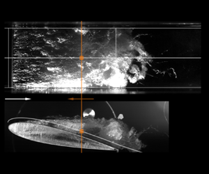
Simultaneous acoustic measurements and high-speed recordings with a dual-camera system were carried out to determine cavity sheet length $\hat {a}$ and thickness $h_0$, and shedding frequencies as well as the power spectral density (PSD). A Brüel & Kjær (B&K) hydrophone type 8103 with a B&K conditioning amplifier type 2650 is flush mounted on the sidewall in a chamber. These data were recorded using a NI cDAQ-9189 chassis with a $16$-bit NI 9223 voltage input module at a sampling rate of 200 kHz for a sampling time of 20 s to obtain clear spectra. The hydrophone signal is used similar to Smith et al. (2020) to calculate the PSD and generate a Welch spectrogram, figure 2(a), choosing a Hanning window with a window size of $20\,000$ or 0.1 s and an overlap of $50\,\%$. The top and side views were recorded simultaneously to the acoustics by a Photron Fastcam Nova S12 operated at a frame rate of 18 000 fps with a spatial resolution of 0.078 mm px$^{-1}$ and an IDT MotionPro Y7 S3 operated at the same synchronised frame rate and a spatial resolution of 0.035 mm px$^{-1}$, respectively. A total of $8001$ frames were stored, resulting in a recording time of 0.45 s. Illumination was provided by two triggered Veritas Constellation 120 LED lights and one IDT 19-LED.

4. Experimental validation and discussion

The Welch spectrogram, cf. figure 2(a), provides an overview of the cavitation regimes manifested throughout the variation of the cavitation number $\sigma$. Three regimes can be distinguished: I sheet cavitation, II re-entrant flow-driven cloud cavitation and III shockwave-driven cloud cavitation. The high-frequency shedding is correlated with II, wherein the frequency exhibits an increase with an increase in $\sigma$ or a decrease in $\hat {a}$. Here, the low-frequency shedding is associated with III. The shedding frequency is independent of $\sigma$. An overlapping region of both frequency bands is evident from $\sigma =1.8$ up to $2.5$.

We first compare the experimentally determined sheet length with the model from § 2.1. Based on the experimental data, the square of the non-dimensionalised nucleation rate $(\,{f_{0}} \,R_0/{U_\infty })^2$ is determined to be ${1.12}$ and supported by its $95\,\%$ confidence interval of $\pm 0.05$. This is of the same order of magnitude as derived in § 2.1. We achieve a good agreement for the asymptotic sheet length between the experiments and the analytical model, figure 2(b). The $95\,\%$ confidence interval of the asymptotic sheet length, represented by the grey-filled area in figure 3(b), is quantified through a Monte Carlo simulation that assumes a Gaussian distribution for the nucleation rate. The experimentally determined asymptotic sheet length is deduced from the top view of the high-speed imaging and the error bar represents the standard deviation across each cycle.

Figure 3. Re-entrant flow dynamics for cavitation numbers in the range between $\sigma =2$ and $4$. (a) Solution of the differential equation in Pelz et al. (2017), (b) the time $t_+$ when the re-entrant flow reaches the leading edge. The Jupyter notebook for producing the figure can be found at https://www.cambridge.org/S0022112024012242/JFM-Notebooks/files/figure_3/figure_3.ipynb.

We can now anticipate the transition from re-entrant flow to shockwave-driven cloud cavitation. The critical cavitation number ${\sigma _\mathrm {II,III}}$ associated with the transition can be calculated from (2.2) as ${\sigma _\mathrm {II,III}} = {1.77}$, denoted by the dashed vertical line in figure 2(a–d). The $95\,\%$ confidence interval of the critical cavitation number ${\sigma _\mathrm {II,III}}$, represented by the grey-filled area, is determined by a Monte Carlo simulation where the upper and lower bounds are $1.69$ and $1.85$, respectively. The prediction seems valid, since the high-frequency shedding associated with the re-entrant flow diminishes close to the predicted value, figure 2(a). A supplementary movie, available at https://doi.org/10.1017/jfm.2024.1224, shows the initiation of the shockwave for $\sigma =1.6$. The shockwave speed in this movie is $U_{S}/U_\infty \approx 0.83$, which matches the values calculated by Bhatt et al. (2023) for the shockwave-driven cloud cavitation regime.

It should be clarified that, in the overlapping region, $\sigma = 1.8$ to $2.5$, both the high- and low-frequency bands, associated with re-entrant flow and condensation shockwaves, respectively, are evident. As the cavitation number decreases further, the low-frequency band intensifies, indicating that the shedding becomes more dominated by shockwaves rather than re-entrant flow. This observation aligns with the recent findings of Bhatt et al. (2023), which provide valuable insights into these complex and multimodal cloud cavitation mechanisms by introducing a probabilistic approach.

A new insight reported here is that, when the sheet reaches the trailing edge, there is a transition from re-entrant flow to shockwave. This transition is clearly visible in figure 2(a). Hence, the new findings are consistent with previous ones, but give a clearer picture of transient cloud cavitation.

Next, we determine the constant $C$, see § 2.2. From the experiment, the average time for the sheet to reach its maximum is $\bar {\tau }_{s} = \overline {{U_\infty }/\dot {a}}\approx 2.38$, cf. figure 2(d).

The re-entrant flow position $\xi (t)/\hat {a}$ over the non-dimensionalised time $t_+:= t{U_\infty } / \hat {a}$ is shown in figure 3(a), illustrating a growth pattern with a discernible peak before converging towards the asymptotic solution. An arrest of the re-entrant flow is experimentally reported by Venning et al. (2022), providing empirical support for the analytically derived kinematics.

It should be noted that, while the re-entrant flow momentum would theoretically be sufficient to extend upstream beyond the cavity leading edge, as indicated by $\xi /\hat {a} > 1$, this is not feasible in practice. Instead, when the re-entrant flow reaches the cavity leading edge, it triggers the formation of a cavitation cloud, which is then advected downstream.

The average time for the re-entrant flow to reach the cavity leading edge, i.e. $\xi /\hat {a}=1$, is $\bar {\tau }_{r}=0.57$, cf. figure 3(b). The mean velocity of the re-entrant flow is $1.75 {U_\infty }$. Experimental findings by Pham et al. (1999) indicate re-entrant flow velocities ranging from $1.1$ to $0.5$ times the free-stream velocity, decreasing with distance from the cavity closure. Callenaere et al. (2001) and Gawandalkar & Poelma (2022) observed velocities around $0.5$ of the velocity at the narrowest cross-section, corresponding to ${U_0}$ in this study. We obtain for the average re-entrant flow velocity $0.88 {U_0}$, being consistent with the values reported in the literature. However, the initial velocity is likely overestimated.

Substituting the average times $\bar {\tau }_{s}=2.38$ and $\bar {\tau }_{r}=0.57$ in (2.3) leads to ${St \approx {0.34} {L_{0}}/\hat {a}}$. The value $C={0.34}$ falls within the range of $1/4$ and $2/5$ reported in the literature. To compare this result with the experiments, we identify the Strouhal numbers of the fundamental modes from the high-speed imaging by applying spectral proper orthogonal decomposition, cf. Sieber, Paschereit & Oberleithner (2016), which provides us with the corresponding standard deviation, shown as error bars in figure 2(c). The identified Strouhal numbers match with the Welch spectrogram in figure 2(a). The constant $C$ is determined from the experiments to be ${0.42}$ through linear regression, which yields a high coefficient of determination $r^2=99.92\,\%$, being larger than ${0.34}$ as calculated from the model. This difference arises from the assumption that the whole cycle duration $\tau$ is the sum of the time required for the sheet growth and the re-entrant flow development. In the experiments, the re-entrant flow already develops during sheet growth, leading to a higher Strouhal number, as predicted. Despite the simplicity of our model, the obtained value is reasonable.

5. Conclusions

The transition from re-entrant flow-driven to shockwave-driven cloud cavitation, as well as the determination of the Strouhal number for re-entrant flow-driven cavitation, were investigated for a NACA 0015 hydrofoil at a fixed Reynolds number and incidence, and varying cavitation number covering the regimes from shockwave-driven cloud cavitation (III), re-entrant flow-driven cloud cavitation (II) and sheet cavitation (I). High-speed imaging as well as high-frequency acoustic measurements using a hydrophone were conducted.

Regime II is associated with a high-frequency shedding which depends on the cavitation number, whereas regime III is associated with the low-frequency shedding independent of it. An overlapping region has been identified where both re-entrant flow and shockwave-driven cloud cavitation coexist, which aligns with the probabilistic approach presented in the recent study by Bhatt et al. (2023). As the cavitation number is reduced further, re-entrant flow-driven cavitation diminishes, and shockwave-driven cloud cavitation becomes the dominant mechanism. This transition occurs when $\hat {a}/L = 1$.

We derived the critical cavitation number ${\sigma _\mathrm {II,III}}$, where the transition from regime III to II occurs, expanding our previous work on the transition from sheet to cloud cavitation (Pelz et al. 2017). Our experimental findings support the hypothesis, i.e. $\hat {a}/L=1$; the high-frequency shedding diminishes at approximately the predicted value ${\sigma _\mathrm {II,III}}$. This offers a new understanding of the transition from re-entrant flow to shockwave-driven cloud cavitation for lifting surfaces, enabling more accurate predictions of this transition.

Despite the hypothesis suggesting that the abrupt stagnation of the sheet, cf. Ganesh (2015), or the adverse pressure gradient, cf. Budich et al. (2018), might trigger the shockwave, the discontinuous pressure distribution at the leading edge for a hydrofoil presents another mechanism to initiate the shockwave.

Next, the parameter $C$ is derived to predict the Strouhal number $St = C {L_{0}} / \hat {a}$; $C$ is found to be ${0.34}$, whereas ${0.42}$ is estimated from a linear regression. Despite the simplicity of our model, the obtained value is reasonable and lies within the reported range: $1/4$ and $2/5$. This simple approach offers valuable new insights into the dynamics of the re-entrant flow, a key mechanism among the two principal drivers of cloud cavitation, facilitating a comprehensive understanding of its dynamic behaviour.