Reconstruction of the 3-D fields with a depth-averaged model for open-channel flows in the smooth turbulent case

Abstract

A two-dimensional depth-averaged model is derived for open-channel flows in the smooth turbulent case. The derivation is consistently obtained with a method of matched asymptotic expansions in the outer and inner layers using a mixing length model of turbulence including the free-surface reduction of the eddy viscosity. The shear effects are taken into account by an extra tensor variable of the model called the enstrophy tensor. The friction coefficient is an explicit expression of the water depth. The three-dimensional velocity field and the friction velocity can be reconstructed from the values of the depth-averaged quantities. Numerical simulations show that the enstrophy can be used to evaluate the development of the turbulent boundary layer. In the case of subcritical unsteady flows, the reconstructed velocity can be described with a logarithmic law modified by Coles’ wake function with apparent von Kármán constant, integration constant and wake-strength parameter, which differ from their values in steady flows. In the viscous sublayer the steady-state relation between the velocity and the vertical coordinate, in the inner scaling, is not valid for unsteady flows. Large errors on the calculation of the von Kármán constant can be made if the validity of the steady-state relation is assumed for unsteady flows. The comparisons of the reconstructed velocity profiles in the case of one-dimensional unsteady open-channel flows and two-dimensional wide trapezoidal channels show a good agreement with experiments.

1. Introduction

The usual equations of open-channel hydraulics in the unsteady case are the one-dimensional (1-D) Saint-Venant equations, also called the nonlinear shallow-water equations. They can be easily extended to the two-dimensional (2-D) case. These equations are derived with the shallow-water assumption, i.e. the water depth is small compared with the characteristic length in the direction parallel to the bottom. As a consequence, at the leading order, the pressure is hydrostatic. Another assumption is that all shear effects are neglected, which means that the velocity is supposed to be uniform over the depth. With these assumptions, the Saint-Venant equations can be derived from the Euler equations of incompressible and inviscid fluids with a depth-averaging procedure.

Except in the case of discontinuities, which are created in finite time due to the hyperbolic structure of the equations, there is no inherent dissipative effects in this approach, which implies that they must be added empirically, most often as an empirical friction force. The Kármán–Prandtl relation for smooth pipes can be extended with slightly different numerical values to the case of smooth open channels but the friction coefficient is found only implicitly. Approximate relations were proposed to obtain an explicit expression of the friction coefficient. More details can be found in Chow (1959) or Yen (2002) for example.

To find the expression of the friction force, or more generally of the dissipative terms, as part of the derivation process of the depth-averaged equations implies taking into account the mean flow and turbulence structure of the flow. Experimental investigation for open-channel flows is more recent than for turbulent boundary layers in close channels because turbulence measurements are more difficult in water than in air flows, and they actually started with the advent of laser Doppler anemometers (Steffler, Rajaratnam & Peterson 1985; Nezu & Rodi 1986). The structure of fully developed open-channel flows is similar to boundary layers and pipe flows, with an inner region controlled by the kinematic viscosity $\nu$ and by the friction velocity $u_b=\sqrt {\tau _b/\rho }$, where $\tau _b$ is the shear stress at the bottom and $\rho$ the fluid density, and an outer region controlled by the water depth $h$ and the maximum velocity. These regions overlap in a layer where the logarithmic law holds. Denoting by $u$ the mean velocity and by $z$ the vertical coordinate, this log law can be written as

(1.1)\begin{equation} u^{+}=\frac{1}{\kappa}\ln {z^{+}} + B,\end{equation}

where $u^{+}=u/u_b$, $z^{+}=zu_b/\nu$, $\kappa$ is the von Kármán constant and $B$ the integration constant. In the outer layer a deviation from the log law can be taken into account by Coles’ wake function (Coles 1956)

(1.2)\begin{equation} u^{+}=\frac{1}{\kappa}\ln {z^{+}} + B + \frac{2 \varPi}{\kappa}f(z/h),\end{equation}

where $h$ is fluid depth and $f$ a universal function often chosen as $f(Z)=\sin ^2 ({\rm \pi} Z/2)$. However, the wake-strength parameter $\varPi$ controlling this function is smaller than for zero-pressure-gradient boundary layers and is nearly equal to zero at a relatively low Reynolds number (Nezu & Rodi 1986). Cardoso, Graf & Gust (1989) found only a weak wake and noted that an apparent log law can approximate the entire velocity profile. If the Froude number, defined by $F=u/\sqrt {gh}$, is smaller than 1, the flow is said to be subcritical (the surface waves are faster than the flow velocity). If $F>1$, the flow is supercritical (no surface perturbation can propagate upstream). For subcritical flows, the measured values of $\kappa$ and $B$ are respectively $0.412$ and $5.29$ (Nezu & Rodi 1986). Very close values were obtained by Cardoso et al. (1989). In the case of supercritical flows, the same value of $\kappa \simeq 0.41$ was measured but it was found that $B$ decreases if the Froude number increases above 1 (Tominaga & Nezu 1992; Prinos & Zeris 1995). Miguntanna et al. (2020) found that the integration constant $B$ is a function of the channel aspect ratio.

In the framework of the eddy viscosity assumption, the mixing length approach (Prandtl 1925) has been extensively applied to open-channel flows and is widely recognized as able to provide an accurate description of the flow over a smooth plane. In the inner layer the mixing length satisfies the classical linear layer modified by the Van Driest damping function (Van Driest 1956). An expression of the mixing length for open-channel flows, including the wake-strength parameter, was obtained by Nezu & Rodi (1986) giving a reduction of the eddy viscosity near the free surface where the mixing length is equal to zero.

In the unsteady case the difficulty is the determination of the friction velocity. Various methods were used and, in particular, the friction velocity can be extracted from velocity measurements in the viscous sublayer assuming the validity for unsteady flows of the law $u^{+}=z^{+}$ that is found in the viscous sublayer in the steady case. The value of the von Kármán constant remains close to $\kappa \simeq 0.41$ for weakly unsteady flows (Nezu, Kadota & Nakagawa 1997) but can deviate from the steady-case value for a strong unsteadiness (Onitsuka & Nezu 2000; Nezu & Onitsuka 2002). Considerable variations of the integration constant $B$ and also of the wake-strength parameter $\varPi$ were found.

The present study is a continuation of a previous work (Richard, Rambaud & Vila 2017) where a new model for open-channel flows was derived using a mixing length model of turbulence and a method of matched asymptotic expansions. In this paper the work is improved and extended on the following points.

1. (i) The mixing length expression of Nezu & Rodi (1986) with the free-surface damping effect is used.

2. (ii) This expression of the mixing length enables an accurate reconstruction of the velocity field from the bottom to the free surface using the calculated depth-averaged quantities.

3. (iii) The model is extended to the case of three-dimensional (3-D) flows, leading to a 2-D depth-averaged model.

4. (iv) The effects of the corrective first-order terms obtained consistently by an asymptotic method are evaluated in unsteady flows with comparisons to experimental results from the literature on the development of the turbulent boundary layer and on unsteady velocity profiles.

The governing equations, the assumptions and the scaling are given in § 2. The asymptotic expansions in the outer and inner layers and the matching procedure are presented in § 3. The depth-averaged model is consistently derived in § 4 using the asymptotic expansions. The method to reconstruct the bottom friction and the 3-D velocity fields is given in § 5. Numerical simulations are presented in § 6 to study the development of the turbulent boundary layer and the velocity profiles in unsteady situations. Technical details are given in the appendices.

2. Governing equations

2.1. Turbulence model

We study a turbulent flow on a sloping channel with a smooth bottom. The angle between the channel and a horizontal plane is $\theta$. The basis for the coordinates $x$, $y$ and $z$ is $(\boldsymbol {e_x},\boldsymbol {e_y},\boldsymbol {e_z})$. The angle between the axis $Ox$ and the fall line is $\beta$ and the axis $Oz$ is normal to the bottom (see figure 1). In these axes the components of the gravity acceleration are $\boldsymbol { g}=g( \sin \theta \cos \beta, \sin \theta \sin \beta,- \cos \theta )^{\mathrm {T}}$.

Figure 1. Definition sketch.

The turbulence is modelled with the mixing length model. The viscous stress tensor is written as $\boldsymbol {\tau }=2\rho (\nu + \nu _T ) \boldsymbol{\mathsf{D}}$, where $\rho$ is the fluid density, $\nu$ its kinematic viscosity, $\nu _T$ the turbulent viscosity. The tensor $\boldsymbol{\mathsf{D}}$ is the strain-rate tensor defined by $\boldsymbol{\mathsf{D}} =[\textbf {grad}\, \boldsymbol v + (\textbf {grad}\, \boldsymbol v )^{\mathrm {T}} ]/2$, where $\boldsymbol v$ is the mean velocity field. The turbulent viscosity is given by $\nu _T = \sqrt {2} L_m^2 \sqrt {\boldsymbol{\mathsf{D}} : \boldsymbol{\mathsf{D}}}$, where the colon denotes the double dot product. For open-channel flows, the mixing length $L_m$, in the model of Prandtl modified by the damping term of Van Driest (1956), if the wake-strength parameter is zero or can be neglected, is given by the expression (Nezu & Rodi 1986),

(2.1)\begin{equation} L_m = \kappa z (1- \mathrm{e}^{{-}z^+{/} A^+})\sqrt{1-\frac{z}{h}}, \end{equation}

where $\kappa$ is the von Kármán constant ($\kappa \simeq 0.41$), $A^+$ is a dimensionless constant with the usual value $A^+=26$ and $h$ is the fluid depth. The dimensionless variable $z^+$ is the viscous or wall coordinate defined by $z^+ = zu_b/\nu$ where the shear or friction velocity $u_b$ is related to the bottom shear stress $\tau _b$ by $u_b = \sqrt {\tau _b/\rho }$. The factor $\sqrt {1-z/h}$ was absent in the expression of the mixing length used by Richard et al. (2017) and, consequently, the velocity profile was accurate only in the inner layer. We define the effective viscosity as $\nu _{{eff}}=\nu + \nu _T$. The constitutive law can thus be written as $\boldsymbol \tau = 2 \rho \nu _{{eff}} \boldsymbol{\mathsf{D}}$.

The wake-strength parameter $\varPi$ of Coles’ law of the wake was found to be considerably smaller in the case of open-channel flows than in the case of zero-pressure-gradient boundary layers where the value $\varPi =0.55$ is observed. Nezu & Rodi (1986) found that $\varPi$ is near zero for $Re \leqslant 10^4$ and increases to a maximum of $0.2$ for $Re \geqslant 2.5 \times 10^4$ (our definition of the Reynolds number is $Re=hU/\nu$, different from the definition of Nezu & Rodi 1986). Cardoso et al. (1989) found a wake of limited strength ($\varPi \simeq 0.08$) in the core of the outer region but they found that the wake effect is partly compensated in the near-surface zone by a retarding flow, such that an apparent logarithmic law can approximate the entire velocity profile, explaining why the logarithmic law is often used with success in an open-channel flow up to the water surface. They also highlighted that the outer region of an open-channel flow may not have a universal structure, possibly depending on secondary currents, flow history and inactive turbulence components. Given the small importance of the wake function in open-channel flows and the large increase of complexity needed to take it into account, the wake function is neglected. However, we will show in the following that, although no wake function is included in the description of uniform and steady flows, an apparent wake function appears in the unsteady case.

The mass conservation equation in the incompressible case is $\mathrm {div}\, \boldsymbol {v} =0$. The components of the velocity field are denoted by $\boldsymbol v=(u,v,w)^{\mathrm {T}}$. The components of the viscous stress tensor are denoted by $\tau _{xx}$, $\tau _{yy}$, $\tau _{zz}$, $\tau _{xy}$, $\tau _{xz}$ and $\tau _{yz}$ and $p$ denotes the pressure. The momentum balance equation is

(2.2)\begin{equation} \rho \left[\frac{\partial \boldsymbol{v}}{\partial t}+ \textbf{div} \left(\boldsymbol{v} \otimes \boldsymbol{v} \right) \right] =\rho \boldsymbol{g}-\textbf{grad} \,p+\textbf{div} \, \boldsymbol{\tau}. \end{equation}

The no-penetration and no-slip conditions at the bottom imply that $\boldsymbol {v}(0)=\boldsymbol {0}$. At the free surface, the kinematic boundary condition is

(2.3)\begin{equation} w(h)=\frac{\partial h}{\partial t}+u(h)\frac{\partial h}{\partial x}+v(h) \frac{\partial h}{\partial y}, \end{equation}

and the dynamic boundary condition gives the following equations:

(2.4)$$\begin{gather} {[}p(h)-\tau_{xx}(h)]\frac{\partial h}{\partial x}- \tau_{xy}(h)\frac{\partial h}{\partial y}+ \tau_{xz}(h)=0, \end{gather}$$

(2.5)$$\begin{gather}{[}p(h)-\tau_{yy}(h)]\frac{\partial h}{\partial y}- \tau_{xy}(h)\frac{\partial h}{\partial x}+\tau_{yz} (h)=0, \end{gather}$$

(2.6)$$\begin{gather}-\tau_{xz}(h)\frac{\partial h}{\partial x}-\tau_{yz}(h) \frac{\partial h}{\partial y}-p(h)+\tau_{zz}(h) =0. \end{gather}$$

2.2. Shallow-water scaling

The equations are written in dimensionless form using a characteristic depth $h_N$, a characteristic length $L$ in the $Ox$ direction and a characteristic velocity $u_N$ with the shallow-water hypothesis

(2.7)\begin{equation} \varepsilon = \frac{h_N}{L}\ll 1. \end{equation}

The dimensionless quantities are denoted with a prime and are defined as

(2.8)\begin{align} \left.\begin{array}{c} x'=\dfrac{x}{L}; \quad y'=\dfrac{y}{L} ; \quad z'=\dfrac{z}{h_N} ; \quad u'=\dfrac{u}{u_N} ; \quad v'=\dfrac{v}{u_N} ; \quad w'=\dfrac{w}{\varepsilon u_N}; \quad p'=\dfrac{p}{\rho g h_N}; \\ t'=\dfrac{tu_N}{L} ; \quad h'=\dfrac{h}{h_N} ; \quad L'_m=\dfrac{L_m}{\kappa h_N} ; \quad \nu'_T = \dfrac{\nu_T}{\kappa^2 h_N u_N} ; \quad \tau'_{xz}=\dfrac{\tau_{xz}}{ \rho \kappa^2 u_N^2} ; \quad \tau'_{yz}=\dfrac{\tau_{yz}}{ \rho \kappa^2 u_N^2} ; \\ \tau'_{xx}=\dfrac{\tau_{xx}}{\varepsilon \rho \kappa^2 u_N^2} ; \quad \tau'_{yy}=\dfrac{\tau_{yy}}{\varepsilon \rho \kappa^2 u_N^2} ; \quad \tau'_{zz}=\dfrac{\tau_{zz}}{\varepsilon \rho \kappa^2 u_N^2} ; \quad \tau'_{xy}=\dfrac{\tau_{xy}}{\varepsilon \rho \kappa^2 u_N^2}. \end{array}\right\}\end{align}

A characteristic turbulent viscosity is $\nu _e=\kappa ^2 h_N u_N$. We define the Froude number $F$, the Reynolds number $Re$ and the mixing length Reynolds number $Re_{{ML}}$ as

(2.9a–c)\begin{equation} F=\frac{u_N}{\sqrt{gh_N}} ; \quad Re=\frac{h_N u_N}{\nu} ; \quad Re_{{ML}}=\frac{h_N u_N}{\nu_e}=\frac{1}{\kappa^2}. \end{equation}

There is no assumption on the Froude number, i.e. $F=O(1)$. We then define the ratio

(2.10)\begin{equation} \eta = \frac{Re_{{ML}}}{Re}=\frac{1}{\kappa^2 Re}=\frac{\nu}{\nu_e}. \end{equation}

This number is usually very small in open-channel hydraulics. We will assume that

(2.11)\begin{equation} \eta=\varepsilon^{2+m} , \quad m>0.\end{equation}

This implies that the Reynolds number must be large for the model to be valid. Specifically, this condition is necessary for the validity of the matching procedure and of the viscous scaling (see below). The validity of the shallow-water scaling does not necessitate a so large Reynolds number. The smooth turbulent regime is valid as long as the shear Reynolds number defined by $Re_b=k_s u_b/\nu$ is smaller than 4 (Henderson 1966), where $k_s$ is the equivalent sand roughness height. This gives a maximum value of $k_s$ compatible with the assumption of a smooth turbulent regime. Taking $F=O(1)$ implies also that $\sin \theta = O[(\ln \eta )^{-2}]$ (see below). The dimensionless mixing length is $L'_m\simeq z' \sqrt {1-s}$, where $s=z/h$ and the effective viscosity is $\nu '_{{eff}}=\nu /\nu _e+\nu '_T=\eta +\nu '_T$. Using $\nu _T = \sqrt {2}\, L_m^2 \,\sqrt {\boldsymbol{\mathsf{D}} : \boldsymbol{\mathsf{D}}}$ and given that $\nu _{{eff}}$ is scaled as $\nu _T$ (see (2.8)) leads to

(2.12)\begin{equation} \nu'_{{eff}}=z'^2 (1-s)\sqrt{\left(\frac{\partial u'}{\partial z'}\right)^2+\left(\frac{\partial v'}{\partial z'}\right)^2} +O(\varepsilon^2). \end{equation}

Note that the term $\exp (-z^+/A^+)$ is negligible in the shallow-water scaling since the full expression is

(2.13)\begin{equation} L'_m=z' \sqrt{1-s} \left[1- \exp \left(-\frac{z' \sqrt{\tau'_b}}{\eta \kappa A^+}\right)\right] \simeq z' \sqrt{1-s}. \end{equation}

We define

(2.14)\begin{equation} \lambda = \frac{\sin \theta}{\kappa^2 F^2}.\end{equation}

The molecular viscosity is negligible in this scaling. In this scaling the mass balance equation reads

(2.15)\begin{equation} \frac{\partial u'}{\partial x'}+ \frac{\partial v'}{\partial y'}+\frac{\partial w'}{\partial z'}=0. \end{equation}

Defining the 2-D vectors $\boldsymbol {u'}=(u',v')^{\mathrm {T}}$, $\boldsymbol {\lambda }=\lambda (\cos \beta, \sin \beta )^{\mathrm {T}}$ and $\boldsymbol {\tau _{sh}}=(\tau _{xz},\tau _{yz})^{\mathrm {T}}$, the momentum balance equation in the $Oxy$ plane becomes

(2.16)\begin{equation} \frac{\varepsilon}{\kappa^2} \left[\frac{\partial \boldsymbol{u'}}{\partial t'}+ \textbf{div} ( \boldsymbol{u'}\otimes \boldsymbol{u'} )+\frac{\partial w' \boldsymbol{u'}}{\partial z'}\right] =\boldsymbol{\lambda}+\frac{\partial \boldsymbol{\tau'_{sh}}}{\partial z'} - \frac{\varepsilon}{\kappa^2 F^2} \textbf{grad} \, p'+O(\varepsilon^2). \end{equation}

In the $Oz$ direction the momentum balance can be written as

(2.17)\begin{equation} \frac{\partial p'}{\partial z'}={-}\cos \theta + O(\varepsilon).\end{equation}

The dynamic boundary conditions at the free surface (2.4)–(2.6) reduce to

(2.18a–c)\begin{equation} p'(h)=O(\varepsilon); \quad \tau'_{xz}(h)=O(\varepsilon^2) ; \quad \tau'_{yz}(h)=O(\varepsilon^2).\end{equation}

As in Richard et al. (2017), in this scaling the boundary condition at the bottom cannot be satisfied. It is necessary to use another scaling in an inner layer near the bottom wall where the molecular viscosity is included.

2.3. Viscous scaling

This scaling is a zoom of the shallow-water scaling using the small parameter $\eta$. Dimensionless quantities in this scaling are denoted by a tilde. Some dimensionless quantities are not changed and some others are magnified. We define

(2.19)\begin{align} \left.\begin{array}{c} \tilde{x}=x' ; \quad \tilde{y}=y' ; \quad \tilde{t}=t' ; \quad \tilde{u}=u' ; \quad \tilde{v}=v' ; \quad \tilde{p}=p' ; \\ \tilde{z}=\dfrac{z'}{\eta} ; \quad \tilde{w}=\dfrac{w'}{\eta} ; \quad \tilde{h}=\dfrac{h'}{\eta} ; \quad \tilde{L}_m = \dfrac{L'_m}{\eta} ; \\ \tilde{\tau}_{xy}=\tau'_{xy} ; \quad \tilde{\tau}_{xz}=\tau'_{xz} ; \quad\tilde{\tau}_{yz}=\tau'_{yz} ; \quad \tilde{\tau}_{xx}=\tau'_{xx} ; \\ \tilde{\tau}_{yy}=\tau'_{yy} ; \quad\tilde{\tau}_{zz}=\tau'_{zz} ; \quad\tilde{\nu}=\dfrac{\nu'}{\eta}. \end{array}\right\} \end{align}

The expression of the dimensionless mixing length in the viscous scaling is

(2.20)\begin{equation} \tilde{L}_m=\tilde{z}\sqrt{1-s}\left[1-\exp\left(- \frac{\tilde{z}\sqrt{\tilde{\tau}_b}}{\kappa A^+}\right)\right]. \end{equation}

In this scaling the exponential term is not negligible since the vertical coordinate is magnified by a factor $\eta$ (but not $\tau _b$) and, consequently,

(2.21)\begin{equation} \exp \left(-\frac{z' \sqrt{\tau'_b}}{\eta \kappa A^+}\right) = \exp \left(-\frac{\tilde{z} \sqrt{\widetilde{\tau_b}}}{ \kappa A^+}\right), \end{equation}

is not small. The dimensionless strain-rate tensor is $\boldsymbol{\tilde {\boldsymbol{\mathsf{D}}}}=\eta \boldsymbol{\mathsf{D}}\boldsymbol{'}$. The dimensionless effective viscosity is $\tilde {\nu }_{{eff}}=1+\tilde {\nu }_T$. This implies that the molecular and turbulent viscosities are of the same order of magnitude in this scaling. The mass conservation is not changed and reads

(2.22)\begin{equation} \frac{\partial \tilde{u}}{\partial \tilde{x}}+\frac{\partial \tilde{v}}{\partial \tilde{y}}+\frac{\partial \tilde{w}}{\partial \tilde{z}}=0. \end{equation}

The momentum balance equation gives

(2.23a–c)\begin{equation} \frac{\partial \tilde{\tau}_{xz}}{\partial \tilde{z}}=O(\eta) ; \quad \frac{\partial \tilde{\tau}_{yz}}{\partial \tilde{z}}=O(\eta) ; \quad \frac{\partial \tilde{p}}{\partial \tilde{z}}=O(\eta).\end{equation}

3. Asymptotic expansions

The methodology is formally the same as in Noble & Vila (2013) for power-law laminar flows and in Richard, Ruyer-Quil & Vila (2016) for laminar Newtonian flows and was detailed in Richard et al. (2017) in the case of 2-D flows. This method is extended to the case of 3-D flows. Each variable is expanded with respect to the small parameter $\varepsilon$ as

(3.1)\begin{equation} X=X_0+\varepsilon X_1 + O(\varepsilon^2) \end{equation}

for any variable $X$. A second small parameter $\mu$ is introduced below and the first-order terms $X_1$ can have additionally an order of magnitude with respect to $\mu$. For example, the first-order correction to the velocity is of $O(\varepsilon /\mu ^2)$. However, the main small parameter governing the asymptotic expansions is still $\varepsilon$ and the second parameter is used only to rank the terms of the highest order (order 1 in the present case). The expansion of the components of the viscous stress tensor will be denoted as $\tau _{xz}=\tau _{xz}^{(0)}+\varepsilon \tau _{xz}^{(1)}+O(\varepsilon ^2)$. The expressions of the variables are obtained at order 0 and then at order 1.

3.1. Order 0

In the shallow-water scaling, the momentum balance equation (2.16) gives

(3.2a,b)\begin{equation} \frac{\partial \tau'^{(0)}_{xz}}{\partial z'}={-}\lambda \cos \beta ; \quad \frac{\partial \tau'^{(0)}_{yz}}{\partial z'}={-}\lambda \sin \beta, \end{equation}

and the boundary conditions (2.18a–c) lead to $\boldsymbol {\tau '^{(0)}_{sh}}(h)=0$. The integration gives

(3.3)\begin{equation} \boldsymbol{\tau'^{(0)}_{sh}}=\boldsymbol{\lambda} h' (1-s ) . \end{equation}

The constitutive law $\boldsymbol {\tau '}=2\nu '_{{eff}}\boldsymbol{\mathsf{D}}\boldsymbol{'}$ gives $\boldsymbol {\tau '^{(0)}_{sh}} = \nu '_{{eff}} \partial \boldsymbol {u'_0}/\partial z'$, which leads to

(3.4)\begin{equation} z'^2 \sqrt{\left(\frac{\partial u'_0}{\partial z'}\right)^2+\left(\frac{\partial v'_0}{\partial z'}\right)^2}\frac{\partial \boldsymbol{u'_0}}{\partial z'}=\boldsymbol{\lambda} h' . \end{equation}

This equation gives the norm

(3.5)\begin{equation} \left\Vert \frac{\partial \boldsymbol{u'_0}}{\partial z'} \right\Vert=\frac{\sqrt{\lambda h'}}{z'}. \end{equation}

The components of $\boldsymbol {u'_0}$ can be integrated between the free surface and an arbitrary depth to obtain

(3.6)\begin{equation} \boldsymbol{ u'_0}=\boldsymbol{u'_0}(h) +\sqrt{\lambda h'}\hat{\boldsymbol{\lambda}} \ln s ,\end{equation}

where $\hat {\boldsymbol {\lambda }}=\boldsymbol {\lambda }/\lambda$. The expression (3.3) does not diverge when $s \to 0$ but the expression (3.6) diverges for $s \to 0$. It is thus necessary to use the viscous scaling to find the expression of the velocity in an inner layer near the bottom. Then a matching procedure will be used in an overlap region to fit the expression of the velocity in the outer layer (with the shallow-water scaling) and in the inner layer (with the viscous scaling).

In the viscous scaling, (2.23a–c) implies that $\tilde {\tau }_{xz}^{(0)}$ and $\tilde {\tau }_{yz}^{(0)}$ are constant in the inner layer and, thus, equal to their values at $z=0$. Since $\boldsymbol {\tilde {\tau }}=\boldsymbol {\tau '}$, and because the expressions of $\tau '^{(0)}_{xz}$ and $\tau '^{(0)}_{yz}$ do not diverge for $z \to 0$, we have simply $\boldsymbol {\tilde {\tau }_{sh}^{(0)}} =\boldsymbol {\tau '^{(0)}_{sh}}(0)= \boldsymbol { \lambda } h'$. We have also $\tilde {\tau }_b= \lambda h'$. The constitutive law is integrated in the viscous scaling in order to find the velocity in the inner layer. With the expression (2.20), the effective viscosity writes in the viscous scaling

(3.7)\begin{equation} \tilde{\nu}_{{eff}}=1+\tilde{z}^2(1-s) (1-\mathrm{e}^{-\tilde{z}\sqrt{\tilde{\tau}_b}/(\kappa A^+)})^2 \sqrt{\left(\frac{\partial \tilde{u}}{\partial \tilde{z}} \right)^2 + \left(\frac{\partial \tilde{v}}{\partial \tilde{z}} \right)^2}. \end{equation}

We define $\xi = 2 \sqrt {\lambda h'}\tilde {z}$ and $A=2\kappa A^+$ to write $\tilde {z}\sqrt {\tilde {\tau }_b}/(\kappa A^+)=\xi / A$ with $\tilde {\tau }_b=\lambda h'$. With $\tilde {\tau }_{xz}^{(0)}=\tilde {\nu }_{{eff}}\partial \tilde {u}_0 / \partial \tilde {z}$ and $\tilde {\tau }_{yz}^{(0)}=\tilde {\nu }_{{eff}}\partial \tilde {v}_0 / \partial \tilde {z}$, the constitutive law gives

(3.8)\begin{equation} \left[1+\tilde{z}^2 (1-s)(1-\mathrm{e}^{-\xi/A})^2 \left\Vert \frac{\partial \boldsymbol{ \tilde{u}_0}}{\partial \tilde{z}}\right\Vert \right]\frac{\partial \boldsymbol{\tilde{u}_0}}{\partial \tilde{z}} =\boldsymbol{\lambda} h' .\end{equation}

From this relation, we can show that

(3.9)\begin{equation} \left\Vert \frac{\partial \boldsymbol{ \tilde{u}_0}}{\partial \tilde{z}}\right\Vert = \frac{2 \lambda h'}{1+\sqrt{1+\xi^2(1-s)(1-\mathrm{e}^{-\xi/A})^2}}. \end{equation}

This can be also written as

(3.10)\begin{equation} \left\Vert \frac{\partial \boldsymbol{ \tilde{u}_0}}{\partial \tilde{z}}\right\Vert = \frac{-1+\sqrt{\varDelta}}{2\tilde{z}^2(1-s)[1-\exp(-\xi/A)]^2}, \end{equation}

with $\varDelta =1+\xi ^2 (1-s)[1-\exp (-\xi /A)]^2$. Inserting this expression in (3.8) leads to

(3.11)\begin{equation} \frac{\partial \boldsymbol{\tilde{u}_0}}{\partial \tilde{z}}=\frac{2 \boldsymbol{\lambda} h' }{1+\sqrt{1+\xi^2(1-s)(1-\mathrm{e}^{-\xi/A})^2}}. \end{equation}

The integration of these equations between the bottom and an arbitrary depth gives

(3.12)\begin{equation} \boldsymbol{\tilde{u}_0}=\sqrt{\lambda h'}\hat{\boldsymbol{\lambda}} \left[-\frac{\xi}{1+\sqrt{1+\xi^2}}+\ln (\xi+\sqrt{1+\xi^2}) +\mathcal{R}(\xi)\right],\end{equation}

where the function $\mathcal {R}$ is defined by

(3.13)\begin{equation} \mathcal{R}(\xi)=\int_0^\xi \frac{\mathrm{d}\xi}{1+\sqrt{1+\xi^2(1-\mathrm{e}^{-\xi/A})^2}} - \int_0^\xi \frac{\mathrm{d}\xi}{1+\sqrt{1+\xi^2}}+O(\sqrt{\eta}). \end{equation}

The limit of this function for $\xi \to \infty$ is denoted by $R$, i.e.

(3.14)\begin{equation} R=\int_0^\infty \frac{\mathrm{d}\xi}{1+\sqrt{1+\xi^2 (1-\mathrm{e}^{-\xi/A})^2}} - \int_0^\infty \frac{\mathrm{d}\xi}{1+\sqrt{1+\xi^2}}. \end{equation}

The vector $\boldsymbol {u'_0}$ in the outer layer and the vector $\boldsymbol {\tilde {u}_0}$ in the viscous layer are fitted by the matching procedure. We write that both velocities coincide in an overlap region that is at a very small depth of order $\sqrt {\eta }$ written as $z=\sqrt {\eta }bh$, where $b=O(1)$. The matching relation can be written as

(3.15)\begin{equation} \boldsymbol{ u'_0}(s=\sqrt{\eta}b)=\boldsymbol{\tilde{u}_0} \left(\xi=\frac{2b\sqrt{\lambda h'^3}}{\sqrt{\eta}}\right)+O(\sqrt{\eta}). \end{equation}

The term of $O(\sqrt {\eta })$ is of an order of magnitude smaller than $\varepsilon$ because of (2.11) ($m>0$). This enables us to obtain consistency at order 1 since the corrective term is of an order smaller than the order 1. This procedure gives the values of the velocity at the free surface $\boldsymbol {u'_0}(h)$. The equation for $\boldsymbol {u'_0}(h)$ can be explicitly written as

(3.16)\begin{align} \boldsymbol{u'_0}(h) + \sqrt{\lambda h'}\hat{\boldsymbol{\lambda}} \ln (b\sqrt{\eta})&=\sqrt{\lambda h'}\hat{\boldsymbol{\lambda}} \left[-\frac{2b\sqrt{\lambda h'^3}}{\sqrt{\eta}} \frac{1}{1+\sqrt{1+4b^2 \lambda h'^3/\eta}} \right. \nonumber\\ &\quad +\ln \left.\left(\frac{2b\sqrt{\lambda h'^3}}{\sqrt{\eta}}+ \sqrt{1+\dfrac{4b^2 \lambda h'^3}{\eta}}\right)+R\right], \end{align}

since $\mathcal {R}(2b\sqrt {\lambda h'^3}/\sqrt {\eta })\simeq R$ (the proof is in Richard et al. (2017)). Neglecting terms of $O(\eta )$, the expression of $\boldsymbol {u'_0}(h)$ can be written as

(3.17)\begin{equation} \boldsymbol{u'_0}(h)=\sqrt{\lambda h'}\hat{\boldsymbol{\lambda}} (R-1+\ln 2 +\ln M - \ln \eta ), \end{equation}

where

(3.18)\begin{equation} M=2\sqrt{\lambda h'^3}.\end{equation}

As in Richard et al. (2017), we introduce the small parameter

(3.19)\begin{equation} \mu ={-}\frac{2}{\ln \eta},\end{equation}

with $\varepsilon < \mu <1$. The main small parameter $\varepsilon$ is smaller than $\mu ^p$ for any positive integer $p$ if $\varepsilon$ is small enough (Richard et al. 2017). Each term of the asymptotic expansions of a given order with respect to $\varepsilon$ is further expanded in a power series of this second small parameter $\mu$. The main relevance of this second small parameter is to neglect some small terms and, especially, the depth average of the cube of the deviation of the velocity from its average value, which is a quantity appearing, in particular, in the energy equation. This is equivalent to Teshukov's approximation of weakly sheared flows (Teshukov 2007). A similar approximation was used by Luchini & Charru (2010) who introduced, after Mellor (1972), the small parameter $u_b/U$, where $U$ is the depth-averaged velocity, which is approximately proportional to $\ln ^{-1}(Re_b)$, where $Re_b=hu_b/\nu$. The deviation of the velocity from its average value was taken into account by terms that were found to be of order $(u_b / U)^2$ while terms of the order of $(u_b / U)^3$ were neglected. The small parameter $u_b / U$ plays the same role as our parameter $\mu$ that can be written as $\mu =2 \ln ^{-1} (\kappa ^2 Re)$. In Appendix B the term $\langle \boldsymbol {u'^{\ast }} \otimes \boldsymbol {u'^{\ast }} \otimes \boldsymbol {u'^{\ast }} \rangle$, where $\boldsymbol {u'^{\ast }}$ is the deviation of the velocity to its average value, is of $O(\mu ^3)$ and can be neglected as in Teshukov (2007).

The expression (3.17) shows that $\boldsymbol {u'_0}(h)$ is of $O(\sqrt {\lambda }/\mu )$. We assume that $\lambda =O(\mu ^2)$. This implies that $\boldsymbol {u'_0}(h)$ is of $O(1)$. With $F=O(1)$, we have $\sin \theta = O(\mu ^2)$. We write $\lambda = \mu ^2 \lambda _0$ with $\lambda _0=O(1)$. The expression of $\boldsymbol {u'_0}(h)$ can be written as

(3.20)\begin{equation} \boldsymbol{u'_0}(h)=\sqrt{\lambda_0 h'}\hat{\boldsymbol{\lambda}} [2+\mu (R-1+\ln 2 +\ln M ) ] . \end{equation}

This gives the complete expressions of $\boldsymbol {u'_0}$ as

(3.21)\begin{equation} \boldsymbol{u'_0}=\sqrt{\lambda_0 h'}\hat{\boldsymbol{\lambda}} [2+\mu (R-1+\ln 2 + \ln M + \ln s )].\end{equation}

At order 0, the velocity has the well-known logarithmic profile. In the 1-D case, reverting to dimensional quantities and introducing the friction velocity, which is $u_b=\sqrt {gh\sin \theta }$, the fluid velocity can be written at order 0,

(3.22)\begin{equation} \frac{u_0}{u_b}=\frac{1}{\kappa}\ln \frac{zu_b}{\nu}+\frac{1}{\kappa}(R-1+2\ln 2 + \ln \kappa ), \end{equation}

which is the usual log law (1.1) with the inner variables $u^{+}=u/u_b$ and $z^{+}=zu_b/\nu$. The expression of the integration constant $B$ is

(3.23)\begin{equation} B=\frac{1}{\kappa}(R-1+2\ln 2 + \ln \kappa ). \end{equation}

The values $\kappa =0.41$ and $A^{+}=26$ give $B=5.28$. These values agree with the value $B=5.29 \pm 0.47$ (and $\kappa =0.412 \pm 0.011$) found by Nezu & Rodi (1986) and with the value $B=5.10 \pm 0.96$ ($\kappa = 0.401 \pm 0.017$) found by Cardoso et al. (1989). The value of $B$ depends on the value of $A^{+}$ through $R$. If $A^{+}=26$ then $R=2.67$. The above values are valid for subcritical flows. For supercritical flows, the value of $B$ can be smaller (Tominaga & Nezu 1992; Prinos & Zeris 1995). This implies smaller values of $A^{+}$ and $R$. The graphs of $R$ and $B$ as a function of $A^{+}$ are shown in figures 2(a) and 2(b), respectively. The dashed lines give the case $A^{+}=26$ used for subcritical flows.

Figure 2. Graphs of $R$ (a) and of the integration constant $B$ (b) as a function of the parameter $A^{+}$ of Van Driest's damping factor. The dashed lines show the case $A^{+}=26$.

Close to the wall, $\xi \to 0$ and $\tilde {u}_0 \sim \xi \sqrt {\lambda h'}/2$. This yields the relation $u^{+}=z^{+}$, which is valid in the viscous sublayer.

Even if the expressions of $u'_0$ and $v'_0$ diverge for $z \to 0$, they are integrable functions on $[0,h]$ and their depth-averaged values can be calculated. For any quantity $X$, its depth-averaged value is defined as

(3.24)\begin{equation} \langle X \rangle=\frac{1}{h}\int_0^h X \, \mathrm{d}z. \end{equation}

The depth-averaged velocity at order 0 can be calculated from (3.21). Using the notation $\boldsymbol {U}=\langle \boldsymbol {u} \rangle =(U,V)^{\mathrm {T}}$, we obtain

(3.25)\begin{equation} \boldsymbol{U'_0} = \sqrt{\lambda_0 h'}\hat{\boldsymbol{\lambda}} [2+\mu (R-2+\ln 2 + \ln M )]. \end{equation}

We define the quantity $C(\mu )$ as

(3.26)\begin{equation} C(\mu)=\frac{U'_0}{\sqrt{\lambda_0 h'}\cos \beta}=\frac{V'_0}{\sqrt{\lambda_0 h'}\sin \beta}. \end{equation}

Its expression is

(3.27)\begin{equation} C(\mu)=2+\mu (R-2+\ln 2+\ln M ).\end{equation}

The velocity in the $Oz$ direction can be found from the mass conservation equation (2.15). Taking into account the kinematic boundary condition, the integration of (2.15) leads to

(3.28)\begin{equation} w'=\frac{\partial h'}{\partial t'}-\frac{\partial}{\partial x'}\int_{h'}^{z'} u' \, \mathrm{d}z'-\frac{\partial}{\partial y'}\int_{h'}^{z'} v' \, \mathrm{d}z'. \end{equation}

The depth-averaged mass conservation equation is

(3.29)\begin{equation} \frac{\partial h}{\partial t}+\frac{\partial hU}{\partial x} + \frac{\partial hV}{\partial y}=0. \end{equation}

With this equation, the derivative of $h'$ with respect to time can be estimated as

(3.30)\begin{equation} \frac{\partial h'}{\partial t'}={-}\frac{\partial h' U'_0}{\partial x'}-\frac{\partial h' V'_0}{\partial y'} + O(\varepsilon). \end{equation}

At order 0, we have

(3.31)\begin{equation} w'_0={-}\frac{\partial h' U'_0}{\partial x'}-\frac{\partial h' V'_0}{\partial y'} +\frac{\partial}{\partial x'}\left(h'\int_{s}^{1} u'_0 \, \mathrm{d}s\right)+\frac{\partial}{\partial y'}\left(h'\int_{s}^{1} v'_0 \, \mathrm{d}s\right), \end{equation}

which leads to

(3.32)\begin{equation} w'_0={-}s\sqrt{\lambda_0 h'}\left(\cos \beta \frac{\partial h'}{\partial x'}+\sin \beta \frac{\partial h'}{\partial y'}\right) \left[1+\frac{\mu}{2}(R-1+\ln 2 +\ln M + \ln s ) \right].\end{equation}

The last quantity to calculate at order 0 is the pressure. It is found from (2.17). The integration is straightforward and gives

(3.33)\begin{equation} p'_0=(h'-z' ) \cos \theta.\end{equation}

In the inner layer, (2.23a–c) implies that $\tilde {p}_0$ is constant. The connection with the expression (3.33) in the outer layer gives simply $\tilde {p}_0=h' \cos \theta$.

3.2. Order 1

The asymptotic expansion at order 1 follows the same procedure as for order 0. The first-order correction to the shear stress is obtained from the momentum balance equation in the shallow-water scaling. Then the integration of the constitutive law gives the first-order correction to the velocity in the outer layer. This expression diverges at the bottom, which necessitates to match this expression with the expression of the first-order correction of the velocity in the inner layer. It is found with the integration of the constitutive law in the viscous scaling. The matching procedure gives the first-order correction to the velocity at the free surface. The integration over the depth of the complete expression of the first-order velocity in the outer layer gives the first-order correction to the depth-averaged velocity. The technical details being much more complicated are gathered in Appendix A.

4. Depth-averaged equations

4.1. Mass and momentum balance equations

The depth-averaged mass conservation equation is given above (3.29). It can be written in vector form using the 2-D divergence operator

(4.1)\begin{equation} \frac{\partial h}{\partial t}+\mathrm{div}\, (h\boldsymbol{U} )=0. \end{equation}

Averaging over the depth the momentum balance equation in dimensionless form in the shallow-water scaling leads to

(4.2)\begin{equation} \frac{\partial h'\boldsymbol{U'}}{\partial t'}+\textbf{div} (h'\langle\boldsymbol{u'}\otimes \boldsymbol{u'}\rangle)+\textbf{grad}\,\left(\frac{h'^2}{2F^2}\cos \theta \right) =\frac{\kappa^2}{\varepsilon}[h'\boldsymbol{\lambda}- \boldsymbol{\tau'_{{sh}}}(0)]+O(\varepsilon).\end{equation}

The expressions (3.3) at order 0 gives $\boldsymbol {\tau '^{(0)}_{{sh}}}(0)=h'\boldsymbol {\lambda }$. The depth-averaged momentum balance equation becomes

(4.3)\begin{equation} \frac{\partial h'\boldsymbol{U'}}{\partial t'}+\textbf{div} (h'\langle\boldsymbol{u'}\otimes \boldsymbol{u'}\rangle) +\textbf{grad}\, \left(\frac{h'^2}{2F^2}\cos \theta \right) ={-}\kappa^2\boldsymbol{\tau'^{(1)}_{{sh}}}(0)+O(\varepsilon). \end{equation}

To calculate the term $\langle \boldsymbol {u'}\otimes \boldsymbol {u'}\rangle$, we define the tensor

(4.4)\begin{equation} \boldsymbol{\varphi} =\frac{\langle(\boldsymbol{u}-\boldsymbol{U})\otimes (\boldsymbol{u}-\boldsymbol{U})\rangle}{h^2}, \end{equation}

which is conveniently called the enstrophy tensor as in Richard, Duran & Fabrèges (2019) because it has the same dimension as the square of a vorticity. By definition we have the equality

(4.5)\begin{equation} \langle\boldsymbol{u}\otimes \boldsymbol{u}\rangle= \boldsymbol{U}\otimes \boldsymbol{U} +h^2 \boldsymbol{\varphi}.\end{equation}

The depth-averaged momentum balance equation can be written as

(4.6)\begin{equation} \frac{\partial h'\boldsymbol{U'}}{\partial t'}+\textbf{div} (h'\boldsymbol{U'}\otimes \boldsymbol{U'}+h'^3\boldsymbol{\varphi'})+\textbf{grad}\, \left(\frac{h'^2}{2F^2}\cos \theta \right) ={-}\kappa^2\boldsymbol{\tau'^{(1)}_{{sh}}}(0)+O(\varepsilon),\end{equation}

with $\boldsymbol {\varphi '}=\boldsymbol {\varphi }h_0^2/u_0^2$. The enstrophy can be expanded as $\boldsymbol {\varphi }=\boldsymbol {\varphi ^{(0)}}+\varepsilon \boldsymbol {\varphi ^{(1)}}+O(\varepsilon ^2)$. The calculation of

(4.7)\begin{equation} \boldsymbol{\varphi'^{(0)}} = \frac{1}{h'^2}\int_0^1 (\boldsymbol{u'_0}-\boldsymbol{U'_0}) \otimes (\boldsymbol{u'_0}-\boldsymbol{U'_0}) \,\mathrm{d}s \end{equation}

yields

(4.8)\begin{equation} \boldsymbol{\varphi'^{(0)}} =\frac{1}{h'}\frac{\boldsymbol{\lambda}\otimes \boldsymbol{\lambda}}{\lambda}. \end{equation}

Writing $\boldsymbol {\lambda }=\mu ^2 \boldsymbol {\lambda _0}$, where $\boldsymbol {\lambda _0}$ is of $O(1)$, the expression of the enstrophy tensor at order 0 can be written as

(4.9)\begin{equation} \boldsymbol{\varphi'^{(0)}} = \frac{\mu^2 \lambda_0}{h'}\frac{\boldsymbol{\lambda}\otimes \boldsymbol{\lambda}}{\lambda^2}=O(\mu^2).\end{equation}

The expressions at order 1 are found from the integral

(4.10)\begin{equation} \boldsymbol{\varphi'^{(1)}} = \frac{1}{h'^2}\int_0^1 [(\boldsymbol{u'_0}-\boldsymbol{U'_0}) \otimes (\boldsymbol{u'_1}-\boldsymbol{U'_1}) +(\boldsymbol{u'_1}-\boldsymbol{U'_1}) \otimes (\boldsymbol{u'_0}-\boldsymbol{U'_0})]\, \mathrm{d}s. \end{equation}

This gives

(4.11)\begin{align} \boldsymbol{\varphi'^{(1)}} &=\frac{\lambda_0}{\kappa^2 h'} \frac{\boldsymbol{\lambda}\otimes \boldsymbol{\lambda}}{\lambda^2} (\hat{\boldsymbol{\lambda}}\boldsymbol{\cdot}\mathbf{grad}\, h' ) \left[1+\frac{\cos \theta}{\lambda_0 F^2}+\mu (R+2+\ln 2 + \ln M - \zeta(3))\right]\nonumber\\ &\quad -\frac{\lambda_0}{\kappa^2 h'}\frac{\cos \theta}{\lambda_0 F^2}( \hat{\boldsymbol{\lambda}} \otimes \mathbf{grad}\, h' +\mathbf{grad}\, h'\otimes \hat{\boldsymbol{\lambda}} )+O(\mu^2). \end{align}

With all expressions of the asymptotic expansions at order 0 and order 1, $\boldsymbol {\tau '^{(1)}_{{sh}}}(0)$ can be consistently written as

(4.12)\begin{align} \boldsymbol{\tau'^{(1)}_{{sh}}}(0) &= \left(1-\alpha_1 \frac{ \mu}{C(\mu)}\right) \frac{\mu^2}{ C^2(\mu)}\left(\Vert \boldsymbol{U'_0} \Vert \boldsymbol{U'_1}+\boldsymbol{U'_0}\frac{\boldsymbol{U'_0}\boldsymbol{\cdot}\boldsymbol{U'_1}}{\Vert \boldsymbol{U'_0} \Vert} \right) \nonumber\\ &\quad -\frac{\alpha}{\kappa^2}\left(\kappa -\alpha_1 \frac{\kappa \mu}{C(\mu)}\right)\frac{\kappa \mu}{C(\mu)}h'^2 \frac{\boldsymbol{\lambda}}{\lambda} \, \mathrm{tr}\, \boldsymbol{\varphi'^{(1)}} + \alpha_1 \frac{\mu}{C(\mu)}h'^2\boldsymbol{\varphi'^{(1)}}\boldsymbol{\cdot}\frac{\boldsymbol{\lambda}}{\lambda}+ O(\mu^3). \end{align}

Quantities of order 1 appear on the right-hand side of this equation. We have

(4.13)\begin{equation} \Vert \boldsymbol{U'_0} \Vert \boldsymbol{U'_1}+ \boldsymbol{U'_0}\frac{\boldsymbol{U'_0}\boldsymbol{\cdot}\boldsymbol{U'_1}}{\Vert \boldsymbol{U'_0} \Vert}= \frac{1}{\varepsilon}(\Vert \boldsymbol{U'}\Vert \boldsymbol{U'}-\Vert \boldsymbol{U'_0}\Vert \boldsymbol{U'_0} )+O(\varepsilon)\end{equation}

and

(4.14)\begin{equation} \boldsymbol{\varphi'^{(1)}}=\frac{1}{\varepsilon}(\boldsymbol{\varphi'} - \boldsymbol{\varphi'^{(0)}} )+O(\varepsilon).\end{equation}

Consequently, $\boldsymbol {\tau '^{(1)}_{{sh}}}(0)$ can be written as a sum of relaxation terms as

(4.15)\begin{align} \boldsymbol{\tau'^{(1)}_{{sh}}}(0) &= \left(1-\alpha_1 \frac{ \mu}{C(\mu)}\right)\frac{\mu^2}{\varepsilon C^2(\mu)} \left(\boldsymbol{U'}\Vert \boldsymbol{U'} \Vert - \frac{C^2(\mu)}{\mu^2}h'\boldsymbol{\lambda} \right) \nonumber\\ &\quad -\frac{\alpha}{\varepsilon\kappa^2} \left(\kappa -\alpha_1 \frac{\kappa \mu}{C(\mu)}\right) \frac{\kappa \mu}{C(\mu)}h' \hat{\boldsymbol{\lambda}} (h' \, \mathrm{tr}\, \boldsymbol{\varphi'}-\lambda)\nonumber\\ &\quad +\frac{ \alpha_1}{\varepsilon} \frac{\mu}{C(\mu)}h' (h'\boldsymbol{\varphi'}\boldsymbol{\cdot}\hat{\boldsymbol{\lambda}} - \boldsymbol{\lambda}) + O(\mu^3), \end{align}

with $\alpha = R_1-R+1$ and

(4.16)\begin{equation} \alpha_1=R_1 -R+1-\frac{1}{2(\zeta(3)-1 )}. \end{equation}

With $\kappa =0.41$ and $A^+=26$, $R=2.67$, $R_1=4.82$, $\alpha = 3.15$ and $\alpha _1=0.680$. The quantity $R_1$ is defined in Appendix A and $\zeta$ is the Riemann zeta function.

In the approximation of weakly sheared flows due to Teshukov (2007), all terms of $O(\mu ^3)$ are neglected (see above and Richard et al. (2017) for a complete discussion).

The quantity $\mu ^2 \kappa ^2 /C^2(\mu )$ is important because it is equal to the friction coefficient (Richard et al. 2017), defined by

(4.17)\begin{equation} C_f = \frac{\mu^2 \kappa^2}{C^2(\mu)}.\end{equation}

This definition of the friction coefficient is obvious when reverting to the dimensional equations (see (4.32) below). The usual Darcy coefficient is $f=8C_f$. From the expression (3.27) of $C(\mu )$, we find that

(4.18)\begin{equation} \frac{1}{\sqrt{C_f}}=\frac{2}{\mu \kappa}+\frac{1}{\kappa}(R-2+\ln 2 + \ln M ). \end{equation}

The definition (3.19) of $\mu$ gives $2/\mu = \ln (\kappa ^2 Re)$. For a uniform and stationary flow, we can take as the characteristic depth and velocity the depth and velocity of the normal (equilibrium) flow. By definition, we have in this case $h'=1$ and $U'=1$. Moreover, for such an equilibrium flow, the first-order corrections are equal to zero. This implies that $U'_0=1$. Since $U'_0=C(\mu )\sqrt {\lambda h'}/\mu$ (see (3.25) and (3.27)), we have at equilibrium $\sqrt {\lambda }=\sqrt {C_f}/\kappa$. Consequently, using the definition (3.18) of $M$, we obtain

(4.19)\begin{equation} \frac{1}{\sqrt{C_f}}=\frac{1}{\kappa}\ln (Re\sqrt{C_f}) + \frac{1}{\kappa}(R-2+2\ln 2 + \ln \kappa). \end{equation}

In open-channel hydraulics the Reynolds number is usually defined with the hydraulic diameter, which is four times the hydraulic radius. The corresponding Reynolds number $Re_H$ can be defined as $Re_H=4Re$ since, in our local approach, the hydraulic radius cannot be defined and is replaced by the depth $h$. Consequently, at equilibrium, for a uniform and stationary flow, the Darcy coefficient $f$ satisfies the implicit relation

(4.20)\begin{equation} \frac{1}{\sqrt{f}}=\frac{\ln 10}{2\kappa \sqrt{2}}\lg (Re_H \sqrt{f}) + \frac{1}{2 \kappa \sqrt{2}}\left(R-2-\frac{3}{2}\ln 2 + \ln \kappa \right). \end{equation}

This relation is similar to the Kármán–Prandtl law for pipe flows with smooth surfaces. The inconvenience of this relation is that the friction coefficient is found only implicitly.

However, in the general case (i.e. equilibrium or non-equilibrium flows), the relation (4.17) leads to the explicit relation

(4.21)\begin{equation} \frac{\kappa}{\sqrt{C_f}}=\frac{2\kappa \sqrt{2}}{\sqrt{f}}=R-2+2\ln 2 + \ln \kappa + \ln \frac{\sqrt{gh^3 \sin \theta}}{\nu}. \end{equation}

With the expression (4.15), the depth-averaged momentum balance equation (4.6) is obtained in a closed conservative form with source terms, which is

(4.22)\begin{align} &\frac{\partial h \boldsymbol{U}}{\partial t}+\mathbf{div} ( h\boldsymbol{U} \otimes \boldsymbol{U} + h^3 \boldsymbol{\varphi}) + \mathbf{grad} \left(\frac{gh^2}{2}\cos\theta \right) =\left(1-\frac{\alpha_1}{\kappa}\sqrt{C_f}\right) (\hat{\boldsymbol{g}}h-C_f \boldsymbol{U} \Vert \boldsymbol{U} \Vert )\nonumber\\ &\quad +\alpha (\kappa-\alpha_1 \sqrt{C_f})h \sqrt{C_f} \frac{\hat{\boldsymbol{g}}}{\hat{g}}\left(h\, \mathrm{tr}\, \boldsymbol{\varphi}-\frac{\hat{g}}{\kappa^2}\right) -\kappa \alpha_1 h\sqrt{C_f}\left(h\boldsymbol{\varphi}\boldsymbol{\cdot}\frac{\hat{\boldsymbol{g}}}{\hat{g}}- \frac{\hat{\boldsymbol{g}}}{\kappa^2}\right), \end{align}

where $\hat {\boldsymbol {g}}$ denotes the projection of the vector $\boldsymbol {g}$ on the plane of the bottom, i.e. $\hat {\boldsymbol {g}} = (g \sin \theta \cos \beta,g \sin \theta \sin \beta ) ^{\mathrm {T}}$ and $\hat {g}=g \sin \theta$. It remains to find an evolution equation for the enstrophy tensor.

4.2. Enstrophy equation

The momentum balance equation in dimensionless form in the shallow-water scaling can be written as

(4.23)\begin{equation} \frac{\partial \boldsymbol{u'}}{\partial t'}+\textbf{div} (\boldsymbol{u'} \otimes \boldsymbol{u'} )+\frac{\partial w'\boldsymbol{u'}}{\partial z'}+\frac{1}{F^2}\textbf{grad}\, p' =\frac{\kappa^2}{\varepsilon}\left( \boldsymbol{\lambda}+\frac{\partial \boldsymbol{\tau'_{{sh}}}}{\partial z'} \right)+O(\varepsilon).\end{equation}

Forming $\boldsymbol {u'} \otimes$(4.23) + (4.23)$\otimes \boldsymbol {u'}$ and averaging the obtained equation over the depth, taking into account the boundary conditions and neglecting all terms of $O(\mu ^3)$ because of the approximation of weakly sheared flows, leads to the equation of the enstrophy tensor. Details on this derivation are given in Appendix B. The result can be written as

(4.24)\begin{align} &\frac{\partial h' \boldsymbol{\varphi'}}{\partial t'}+\mathbf{div}(h' \boldsymbol{\varphi'} \otimes \boldsymbol{U'} ) - 2 h' \boldsymbol{\varphi'} \mathrm{div}\, \boldsymbol{U'} +\mathbf{grad}\, \boldsymbol{U'}\boldsymbol{\cdot}h' \boldsymbol{\varphi'} +h' \boldsymbol{\varphi'}\boldsymbol{\cdot}( \mathbf{grad}\, \boldsymbol{U'} )^{\mathrm{T}}\nonumber\\ &\quad =\frac{\kappa^2}{\varepsilon}\frac{1}{h'^2} [ \boldsymbol{U'} \otimes \boldsymbol{\tau'_{{sh}}}(0)+ \boldsymbol{\tau'_{{sh}}}(0) \otimes \boldsymbol{U'} - 2\boldsymbol{\mathsf{W}} ] +O(\mu^3) +O(\varepsilon), \end{align}

where $\boldsymbol{\mathsf{W}}$ is the dissipation tensor defined by

(4.25)\begin{equation} \boldsymbol{\mathsf{W}}=\int_0^{h'} \nu'_{{eff}} \frac{\partial \boldsymbol{u'}}{\partial z'}\otimes \frac{\partial \boldsymbol{u'}}{\partial z'}\,\mathrm{d}z'. \end{equation}

The dissipation tensor is expanded as $\boldsymbol{\mathsf{W}}=\boldsymbol{\mathsf{W}}_{\boldsymbol {0}}+\varepsilon \boldsymbol{\mathsf{W}}_{\boldsymbol{1}} + O(\varepsilon ^2)$. These asymptotic expansions are given in Appendix B and enable us to write the right-hand side of (4.24) as a sum of relaxation terms.

4.3. Final system of equations

The final system of equations is composed of the mass conservation equation

(4.26)\begin{equation} \frac{\partial h}{\partial t}+\mathrm{div}\, (h\boldsymbol{U} )=0, \end{equation}

the momentum balance equation

(4.27)\begin{align} &\frac{\partial h \boldsymbol{U}}{\partial t}+\mathbf{div} ( h\boldsymbol{U} \otimes \boldsymbol{U} + h^3 \boldsymbol{\varphi}) + \mathbf{grad}\left(\frac{gh^2}{2}\cos\theta \right) =\left(1-\frac{\alpha_1}{\kappa}\sqrt{C_f}\right) (\hat{\boldsymbol{g}}h-C_f \boldsymbol{U}\Vert \boldsymbol{U} \Vert )\nonumber\\ &\quad +\alpha (\kappa-\alpha_1 \sqrt{C_f})h \sqrt{C_f} \frac{\hat{\boldsymbol{g}}}{\hat{g}}\left(h\, \mathrm{tr}\, \boldsymbol{\varphi}-\frac{\hat{g}}{\kappa^2}\right) -\kappa \alpha_1 h\sqrt{C_f}\left(h\boldsymbol{\varphi}\boldsymbol{\cdot}\frac{\hat{\boldsymbol{g}}}{\hat{g}}-\frac{\hat{\boldsymbol{g}}}{\kappa^2} \right) \end{align}

and the enstrophy equation (obtained from Appendix B)

(4.28)\begin{align} &\frac{\partial h \boldsymbol{\varphi}}{\partial t}+\mathbf{div} (h\boldsymbol{\varphi}\otimes \boldsymbol{U}) -2 h\boldsymbol{\varphi} \mathrm{div}\, \boldsymbol{U}+\mathbf{grad}\, \boldsymbol{U}\boldsymbol{\cdot}h \boldsymbol{\varphi}+h\boldsymbol{\varphi}\boldsymbol{\cdot}(\mathbf{grad}\, \boldsymbol{U} )^{\mathrm{T}}\nonumber\\ &\quad =\frac{\alpha_2}{\kappa}\frac{\sqrt{C_f}}{h^2} [\boldsymbol{U} \otimes (C_f \boldsymbol{U} \Vert\boldsymbol{U} \Vert- \hat{\boldsymbol{g}}h)+(C_f \boldsymbol{U} \Vert \boldsymbol{U} \Vert - \hat{\boldsymbol{g}}h)\otimes \boldsymbol{U} ]\nonumber\\ &\qquad -\alpha \alpha_2 \frac{C_f}{h} \left(\boldsymbol{U} \otimes \frac{\hat{\boldsymbol{g}}}{\hat{g}}+ \frac{\hat{\boldsymbol{g}}}{\hat{g}}\otimes \boldsymbol{U} \right) \left(h\, \mathrm{tr}\, \boldsymbol{\varphi}- \frac{\hat{g}}{\kappa^2}\right)\nonumber\\ &\qquad -\kappa \alpha_2 \frac{\sqrt{C_f}}{h}\left[\boldsymbol{U}\otimes \left(h\boldsymbol{\varphi}\boldsymbol{\cdot}\frac{\hat{\boldsymbol{g}}}{\hat{g}}- \frac{\hat{\boldsymbol{g}}}{\kappa^2}\right) +\left(h\boldsymbol{\varphi}\boldsymbol{\cdot}\frac{\hat{\boldsymbol{g}}}{\hat{g}}- \frac{\hat{\boldsymbol{g}}}{\kappa^2}\right)\otimes \boldsymbol{U}\right], \end{align}

where

(4.29)\begin{equation} \alpha_2 = \frac{1}{2(\zeta(3)-1)}. \end{equation}

With $\kappa =0.41$ and $A^+=26$, $\alpha _2=2.47$. Note that $\alpha _1 = \alpha - \alpha _2$. The system has the same mathematical structure as the system derived by Teshukov (2007), with additional source terms, who gave the proof of its hyperbolicity. Shearing effects, i.e. the variations of the velocity in the depth, are taken into account by the anisotropic enstrophy tensor. All source terms are relaxation terms for the average velocity or the enstrophy. Note that the full 2-D system is hyperbolic but not in conservative form due to non-conservative terms in the enstrophy equation.

4.4. Two-dimensional Saint-Venant equations

As implied by (4.9), the enstrophy is of $O(\mu ^2)+O(\varepsilon )$. Furthermore, since $\boldsymbol {U'_1}=O(1/\mu ^2)$ we can write

(4.30)\begin{equation} \boldsymbol{\tau'^{(1)}_{{sh}}}(0) = \frac{\mu^2}{C^2(\mu)}\left( \Vert \boldsymbol{U'_0} \Vert \boldsymbol{U'_1}+\boldsymbol{U'_0}\frac{\boldsymbol{U'_0}\boldsymbol{\cdot}\boldsymbol{U'_1}}{\Vert \boldsymbol{U'_0} \Vert} \right)+O(\mu). \end{equation}

Consequently, the expression (4.15) of $\boldsymbol {\tau '^{(1)}_{{sh}}}(0)$ can be written as

(4.31)\begin{equation} \boldsymbol{\tau'^{(1)}_{{sh}}}(0) = \frac{\mu^2}{\varepsilon C^2(\mu)}\left(\boldsymbol{U'}\Vert \boldsymbol{U'} \Vert - \frac{C^2(\mu)}{\mu^2}h'\boldsymbol{\lambda} \right) + O(\mu). \end{equation}

This equation shows why the quantity $\mu ^2\kappa ^2/C^2(\mu )$ is the friction coefficient $C_f$, which appears clearly when reverting to dimensional form. Neglecting terms of $O(\mu )$, the dimensional depth-averaged momentum balance equation becomes, in dimensional form,

(4.32)\begin{equation} \frac{\partial h \boldsymbol{U}}{\partial t}+\textbf{div} ( h\boldsymbol{U} \otimes \boldsymbol{U} ) + \textbf{grad} \left(\frac{gh^2}{2}\cos\theta \right) =\hat{\boldsymbol{g}}h-C_f \boldsymbol{U} \Vert \boldsymbol{U} \Vert .\end{equation}

At this level of approximation, there is no enstrophy balance equation and the system reduces to the 2-D Saint-Venant equations. The friction term is consistently rather than empirically introduced. Keeping terms up to $O(\mu ^2)$ and neglecting terms of $O(\mu ^3)$ gives the complete system {(4.26), (4.27), (4.28)}.

4.5. Energy equation

The system admits an energy balance equation. Taking half the trace of (B4) in dimensional form gives the energy balance equation

(4.33) \begin{align} &\frac{\partial he}{\partial t}+\mathrm{div}( he\boldsymbol{U}+\boldsymbol{U}\boldsymbol{\cdot}\boldsymbol{\varPi} ) = \left( 1-\frac{\alpha}{\kappa}\sqrt{C_f} \right) (\hat{\boldsymbol{g}}h-C_f\Vert \boldsymbol U \Vert\boldsymbol U )\boldsymbol{\cdot}\boldsymbol U \nonumber\\ &\quad +\alpha (\kappa - \alpha \sqrt{C_f} )h \sqrt{C_f} \left(h \, \mathrm{tr}\, \boldsymbol{\varphi}-\frac{\hat{g}}{\kappa^2}\right) \frac{\hat{\boldsymbol{g}}}{\hat{g}}\boldsymbol{\cdot}\boldsymbol U -\kappa \alpha h \sqrt{C_f}\left(h \boldsymbol{\varphi}\boldsymbol{\cdot}\frac{\hat{\boldsymbol{g}}}{\hat{g}}-\frac{\hat{\boldsymbol{g}}}{\kappa^2} \right)\boldsymbol{\cdot}\boldsymbol U,\nonumber\\ \end{align}

where the specific energy $e$ is

(4.34)\begin{equation} e=\frac{\boldsymbol U\boldsymbol{\cdot}\boldsymbol U}{2}+\frac{gh}{2}\cos \theta + \frac{h^2}{2}\,\mathrm{tr} \,\boldsymbol{\varphi} \end{equation}

and where the tensor $\boldsymbol {\varPi }$ is

(4.35)\begin{equation} \boldsymbol{\varPi}=\frac{gh^2}{2}\cos \theta \boldsymbol{\mathsf{I}} + h^3 \boldsymbol{\varphi}. \end{equation}

In this expression, $\boldsymbol{\mathsf{I}}$ is the identity tensor. The terms on the right-hand side of the energy equation are relaxation terms due to the dissipative effects in the flow. The expression of the turbulent energy of the system is $h^2 \, \mathrm {tr}\, \boldsymbol {\varphi }/2$.

In the particular case of the Saint-Venant equations where the terms of $O(\mu )$ are neglected, the specific energy reduces to

(4.36)\begin{equation} e=\frac{\boldsymbol U \boldsymbol{\cdot}\boldsymbol U}{2}+\frac{gh}{2}\cos \theta, \end{equation}

the tensor $\boldsymbol {\varPi }$ reduces to $\boldsymbol {\varPi }=(gh^2/2)\cos \theta \boldsymbol{\mathsf{I}}$ and the energy balance equation reduces to

(4.37)\begin{equation} \frac{\partial he}{\partial t}+\mathrm{div}( he \boldsymbol{U}+\boldsymbol{U}\boldsymbol{\cdot}\boldsymbol{\varPi} ) = (\hat{\boldsymbol{g}}h-C_f\Vert \boldsymbol U \Vert\boldsymbol U ) \boldsymbol{\cdot}\boldsymbol U . \end{equation}

5. Reconstruction of the 3-D fields

The 3-D fields can be reconstructed from the values of the depth $h$, of the depth-averaged fluid velocity $\boldsymbol {U}$ and of the enstrophy tensor as a function of the applicate $z$ or of $s=z/h$.

The expression of the shear stress at the bottom can be found from the expressions (3.3) at order 0 and (A6) at order 1. At order 0, the expression $\boldsymbol {\tau '^{(0)}_{sh}}(0) = \boldsymbol {\lambda }h$ can be written as $\boldsymbol {\tau '^{(0)}_{sh}}(0) = \mu ^2\boldsymbol {U_0}\Vert \boldsymbol {U_0} \Vert /C^2(\mu )$. The shear stress at order 1 has already been consistently written as a sum of relaxation terms in (4.15). Forming $\boldsymbol {\tau '_{sh}}(0) =\boldsymbol {\tau '^{(0)}_{sh}}(0) +\varepsilon \boldsymbol {\tau '^{(1)}_{sh}}(0)$ and reverting to dimensional quantities leads to the expression of the shear stress at the bottom,

(5.1)\begin{align} \frac{\boldsymbol{\tau_{sh}}(0)}{\rho}&=C_f \boldsymbol{U} \Vert \boldsymbol{U}\Vert -\frac{\alpha_1}{\kappa}\sqrt{C_f} (C_f \boldsymbol{U}\Vert U \Vert - \hat{\boldsymbol{g}}h ) \nonumber\\ &\quad -\alpha (\kappa - \alpha_1 \sqrt{C_f} ) \sqrt{C_f} \frac{\hat{\boldsymbol{g}}}{\hat{g}}h \left(h \, \mathrm{tr}\, \boldsymbol{\varphi}-\frac{\hat{g}}{\kappa^2} \right) +\kappa \alpha_1 \sqrt{C_f}h \left(h \boldsymbol{\varphi}\boldsymbol{\cdot}\frac{\hat{\boldsymbol{g}}}{\hat{g}}- \frac{\hat{\boldsymbol{g}}}{\kappa^2} \right), \end{align}

which is a function of the depth $h$, the average velocity $\boldsymbol {U}$ and the enstrophy tensor $\boldsymbol {\varphi }$, with relaxation terms on these quantities but without any derivative. This expression enables us to calculate very easily the bottom shear stress with the correction of order 1.

From the expressions (3.21) and (3.25), we can write $\boldsymbol {u'_0}=\boldsymbol {U'_0}[1+(\mu /C(\mu ))( 1+ \ln s ) ]$. At order 1, the expressions (A31) and (A33) lead to

(5.2)\begin{align} \boldsymbol{u'_1}&=\boldsymbol{U'_1}\left[1+\frac{\mu}{C} ( 1+ \ln s ) \right] -(1+\ln s )\alpha\frac{\mu^2}{C^2} ( \boldsymbol{U'_1}\boldsymbol{\cdot}\hat{\boldsymbol{\lambda}} ) \hat{\boldsymbol{\lambda}} +\alpha_2\left[\mathrm{Li}_2(1-s) + 1-\frac{{\rm \pi}^2}{6} \right]\nonumber\\ &\quad \times \left[\frac{\mu}{C}(\boldsymbol{U'_1}\boldsymbol{\cdot}\hat{\boldsymbol{\lambda}} )\hat{\boldsymbol{\lambda}} -h'\frac{ \mathrm{tr}\, \boldsymbol{\varphi'_1}}{2\sqrt{\mathrm{tr}\, \boldsymbol{\varphi'_0}}} \hat{\boldsymbol{\lambda}} - \alpha\frac{\mu^2}{C^2}(\boldsymbol{U'_1}\boldsymbol{\cdot}\hat{\boldsymbol{\lambda}} )\hat{\boldsymbol{\lambda}} \right]+O(\mu). \end{align}

Forming $\boldsymbol {u}=\boldsymbol {u^{(0)}}+\varepsilon \boldsymbol {u^{(1)}}$ and reverting to dimensional quantities gives the 3-D reconstruction of the horizontal velocity field in the outer layer, accurate at order 1,

(5.3)\begin{align} \boldsymbol{u}&=\boldsymbol{U}\left[1+\frac{\sqrt{C_f}}{\kappa} \left(1+\ln \frac{z}{h} \right) \right] -\alpha \frac{\sqrt{C_f}}{\kappa^2}\left( \sqrt{C_f} \boldsymbol{U}\boldsymbol{\cdot}\frac{\hat{\boldsymbol{g}}}{\hat{g}}- \sqrt{\hat{g}h } \right)\frac{\hat{\boldsymbol{g}}}{\hat{g}} \left(1+\ln \frac{z}{h} \right)\nonumber\\ &\quad +\alpha_2 \left[1-\frac{{\rm \pi}^2}{6}+ \mathrm{Li_2}\left( 1-\frac{z}{h}\right) \right] \left[\frac{\sqrt{C_f}}{\kappa} \boldsymbol{U}\boldsymbol{\cdot}\frac{\hat{\boldsymbol{g}}}{\hat{g}} - h \sqrt{\mathrm{tr}\, \boldsymbol{\varphi}}\right.\nonumber\\ &\quad \left.-\alpha \frac{\sqrt{C_f}}{\kappa^2}\left( \sqrt{C_f} \boldsymbol{U}\boldsymbol{\cdot}\frac{\hat{\boldsymbol{g}}}{\hat{g}}- \sqrt{\hat{g}h } \right) \right] \frac{\hat{\boldsymbol{g}}}{\hat{g}}. \end{align}

This expression enables us to reconstruct the 3-D profile of the horizontal velocity in the outer layer from the quantities $h$, $\boldsymbol {U}$ and $\boldsymbol {\varphi }$ calculated with the resolution of the 2-D model.

A similar method is conducted in the inner layer. The expressions of the velocity at order 0 and 1 are given in Appendix C. Note that the expression of $\tilde {u}_1$ in the inner layer has to be accurate to within $O(\mu ^2)$ in order to obtain a matching with the expression of $u'_1$ in the outer layer accurate to within $O(\mu )$ when $\xi \to \infty$. In dimensional form the 3-D reconstruction of the horizontal velocity in the inner layer is

(5.4) \begin{align} \boldsymbol{u}&=\frac{1}{\kappa}\left\{ \sqrt{C_f}\boldsymbol{U} +\left[\left(1-2\frac{\alpha}{\kappa}\sqrt{C_f}+2\frac{\alpha \alpha_1}{\kappa^2}C_f \right)\left(\sqrt{C_f} \boldsymbol{U}\boldsymbol{\cdot} \frac{\hat{\boldsymbol{g}}}{\hat{g}} -\sqrt{\hat{g}h}\right)\right.\right.\nonumber\\ &\quad +\left.2\alpha_2\sqrt{C_f}\left.\left(\frac{\sqrt{C_f}}{\kappa} \boldsymbol{U}\boldsymbol{\cdot} \frac{\hat{\boldsymbol{g}}}{\hat{g}}-h \sqrt{\mathrm{tr}\, \boldsymbol{ \varphi}}\right)\right] \frac{\hat{\boldsymbol{g}}}{\hat{g}}\right\} \left[\mathcal{R}(\xi)- \frac{\xi}{1+\sqrt{1+\xi^2}}+\ln(\xi+\sqrt{1+\xi^2}) \right] \nonumber\\ &\quad +\frac{1}{\kappa}\left[\left(1-\frac{\alpha}{\kappa} \sqrt{C_f}+\frac{\alpha \alpha_1}{\kappa^2}C_f \right) \left(\sqrt{C_f} \boldsymbol{U}\boldsymbol{\cdot} \frac{\hat{\boldsymbol{g}}}{\hat{g}}- \sqrt{\hat{g} h}\right)\right.\nonumber\\ &\quad \left.+\,\alpha_2 \sqrt{C_f} \left(\frac{\sqrt{C_f}}{\kappa}\boldsymbol{U}\boldsymbol{\cdot} \frac{\hat{\boldsymbol{g}}}{\hat{g}}-h\sqrt{\mathrm{tr}\, \boldsymbol{ \varphi}}\right)\right]\frac{\hat{\boldsymbol{g}}}{\hat{g}} \nonumber\\ &\quad \times \left[\mathcal{R}_1(\xi)-2\mathcal{R}(\xi)+ \frac{2\xi}{1+\sqrt{1+\xi^2}}-\ln(\xi+\sqrt{1+\xi^2}) \right], \end{align}

with

(5.5)\begin{equation} \xi=\frac{2\kappa}{\nu}z\sqrt{gh\sin \theta}. \end{equation}

This expression is less convenient than the expression in the outer layer because the functions $\mathcal {R}$ and $\mathcal {R}_1$ are not explicit and need to be numerically calculated, but the full 3-D velocity profile, from the bottom to the free surface, can be calculated with the depth-averaged quantities $h$, $\boldsymbol {U}$ and $\boldsymbol {\varphi }$ using the expression (5.4) in the inner layer and the expression (5.3) in the outer layer. These expressions connect asymptotically in the overlap layer with an accuracy of $O(\mu )$. At the equilibrium, the relaxation terms are equal to zero, and these expressions reduce to

(5.6)\begin{equation} \boldsymbol{u}=\boldsymbol{U}\left[1+\frac{\sqrt{C_f}}{\kappa} \left(1+\ln \frac{z}{h} \right) \right] \end{equation}

in the outer layer and to

(5.7)\begin{equation} \boldsymbol{u}=\frac{\sqrt{C_f}}{\kappa} \boldsymbol{U} \left[\mathcal{R}(\xi)-\frac{\xi}{1+\sqrt{1+\xi^2}}+\ln (\xi+\sqrt{1+\xi^2}) \right] \end{equation}

in the inner layer. In the viscous sublayer $\xi \to 0$ and the velocity in the inner layer is equivalent to a linear function of $z$. Defining the friction velocity $u_b=\sqrt {\tau _b/\rho }$, $\boldsymbol {u^{+}}=\boldsymbol {u}/u_b$ and $z^{+}=zu_b/\nu$ and taking $\tau _b=\Vert \boldsymbol { \tau _{sh} } \Vert (0)$, where $\boldsymbol { \tau _{sh} }(0)$ is given by (5.1), we obtain

(5.8)\begin{align} \boldsymbol{u^{+}}&= z^{+}\frac{ \sqrt{gh\sin \theta}}{\Vert\boldsymbol{ \tau_{sh} } \Vert(0)/\rho}\left\{ \sqrt{C_f}\boldsymbol{U} +\left[\left(1-2\frac{\alpha}{\kappa}\sqrt{C_f}+2\frac{\alpha \alpha_1}{\kappa^2}C_f \right)\left(\sqrt{C_f} \boldsymbol{U}\boldsymbol{\cdot}\frac{\hat{\boldsymbol{g}}}{\hat{g}} -\sqrt{\hat{g} h}\right)\right.\right.\nonumber\\ &\quad +\left.\left.2\alpha_2\sqrt{C_f}\left(\frac{\sqrt{C_f}}{\kappa} \boldsymbol{U}\boldsymbol{\cdot}\frac{\hat{\boldsymbol{g}}}{\hat{g}}-h \sqrt{\mathrm{tr}\, \boldsymbol{ \varphi}}\right)\right] \frac{\hat{\boldsymbol{g}}}{\hat{g}}\right\} . \end{align}

In an equilibrium situation the relaxation terms are equal to zero, in particular, $\sqrt {C_f}\Vert \boldsymbol {U} \Vert = \sqrt {\hat {g} h}$, and the previous expression gives $\Vert \boldsymbol {u^{+}} \Vert = z^{+}$ that corresponds to the usual law in the viscous sublayer $u^+=z^+$. In a non-equilibrium situation, in particular, for an unsteady flow, the relation between $u^+$ and $z^+$ is still a linear relation but it is more complex and $u^+ / z^+ \neq 1$.

6. Numerical simulations

6.1. Numerical scheme

The system of (4.26)–(4.28) is a hyperbolic system with relaxation source terms. In the 1-D case it can be written as

(6.1)\begin{equation} \frac{\partial \boldsymbol{\mathcal{U}}}{\partial t}+\frac{\partial \boldsymbol{\mathcal{F}}}{\partial x}=\boldsymbol{\mathcal{S}}, \end{equation}

where $\boldsymbol {\mathcal {U}}=[h,hU,he]^\mathrm {T}$, $\boldsymbol {\mathcal {F}}=[hU,hU^2+\varPi,hUe+\varPi U]^\mathrm {T}$ and

(6.2)\begin{align} \boldsymbol{\mathcal{S}} =\left[\begin{array}{l} 0,\\ \left(1-\dfrac{\alpha_1}{\kappa}\sqrt{C_f}\right) (\hat{g} h-C_f U \vert U \vert )+[\kappa(\alpha-\alpha_1) -\alpha_1 \sqrt{C_f}]h\sqrt{C_f}\left(h\varphi- \dfrac{\hat{g}}{\kappa^2} \right) ,\\ \left(1-\dfrac{\alpha}{\kappa}\sqrt{C_f}\right) (\hat{g} h-C_f U \vert U \vert )U-\alpha^2hC_f \left(h\varphi - \dfrac{\hat{g}}{\kappa^2} \right)U. \end{array} \right. \end{align}

The energy of the system is $e=(U^2+gh\cos \theta +h^2 \varphi )/2$ and $\varPi =(gh^2 \cos \theta ) /2 +h^3 \varphi$. The characteristics of the system are $\lambda _{1,2}=U\pm \sqrt {gh+3h^2 \varphi }$ and $\lambda _3=U$. The friction coefficient $C_f$ is calculated locally with the explicit relation (4.21).

This system is solved with a classical explicit Godunov-type finite-volume method and a Rusanov Riemann solver. The time step is calculated with a Courant–Friedrichs–Lewy (CFL) condition. At each time step, the enstrophy is calculated from the energy.

The system is solved for the simulation of a subcritical flow in an open channel. At the entrance the discharge is prescribed and the flow is supposed to be non-developed. This means that the enstrophy can be taken equal to zero since the velocity is uniform in the depth. If $\varphi =0$ at the entrance, the system reduces to the system of Saint-Venant. The depth in a ghost cell at the entrance is then calculated from the conservation of the Riemann invariant of the Saint-Venant system $U-2\sqrt {gh}$.

The end of the channel is treated as a sharp-crested weir as in Richard & Gavrilyuk (2013): if the depth $h_N$ in the last cell is smaller than some height $d$, which corresponds to the height of the weir, then the discharge $q_{N+1}$ in a ghost cell after the last cell is zero, otherwise $q_{N+1}=(2/3)C_d [2g(h_N-d)^3]^{1/2}$ with $C_d ={\rm \pi} /({\rm \pi} +2)+0.08(h_N-d)/d$ (Henderson 1966). Neumann boundary conditions are taken for the depth and the enstrophy.

The numerical cost of the resolution of this system is slightly larger but of the same order of magnitude as the classical Saint-Venant equations. The additional enstrophy equation is numerically cheap because it is, in one dimension, a simple advection equation with source terms. A more precise evaluation of the numerical cost was done for the resolution of the 2-D system (see § 6.5).

6.2. Development of the boundary layer

Simulations are performed for a uniform flow in a steady case, the so-called normal conditions. The value of the Reynolds number $Re=hU/\nu$ is chosen. The kinematic viscosity is fixed at $\nu =1.0\times 10^{-6}\ \mathrm {m}^2 \, \mathrm {s}^{-1}$. This gives the value $q_n$ of the discharge $q=hU$. The friction coefficient $C_{f\! n}$ for a uniform and steady flow is then calculated with (4.20). The value of the Froude number $F=U/(gh)^{1/2}$ is chosen and the angle $\theta$ is then calculated by $\sin \theta = F^2 C_{f\! n}$ in order to have a normal flow. The average velocity of the normal flow is then found by $U_n = (F^2 g\nu Re )^{1/3}$ and the normal depth $h_n$ is determined as well. The height of the weir $d$ is calculated from the resolution of the equation $(gh_n^3 \sin \theta /C_{f\! n})^{1/2}=(2/3)C_d [2g(h_n-d)^3]^{1/2}$, $C_d$ being calculated with the normal depth.

The discharge $q_n$ is prescribed at the entrance. After a transient regime the system reaches a steady state where the depth and the velocity are $h_n$ and $U_n$ everywhere except near the beginning of the channel. Since $\varphi =0$ is prescribed at the entrance of the channel because the flow is supposed to be non-developed, the enstrophy relaxes towards its equilibrium value. The enstrophy approaches asymptotically its normal value $\varphi _n= g \sin \theta /(\kappa ^2 h_n)$ and, after some distance, the flow is indistinguishable from a normal flow with a fully developed boundary layer. The value of the enstrophy can be used as an evaluation of the development of the boundary layer at the beginning of the channel, with the value $\varphi =0$ for a non-developed flow and the value $\varphi _n$ for a fully developed flow. Assuming that, for a partially developed boundary layer, the velocity profile satisfies the usual logarithmic law below the boundary layer thickness $\delta$ and that it is uniform above this limit up to the free surface, we have

(6.3)\begin{equation} u'_0=\sqrt{\lambda_0h'}\left[ 2+\mu\left(R-1+\ln 2+\ln M+\ln \frac{z}{\delta}\right) \right]\quad \mathrm{if}\ z \leqslant \delta, \end{equation}

and

(6.4)\begin{equation} u'_0=\sqrt{\lambda_0h'}[ 2+\mu(R-1+\ln 2+\ln M) ]\quad \mathrm{if}\ \delta\leqslant z \leqslant h. \end{equation}

Denoting $\varphi _{max}=\varphi (\delta =h)$, this yields

(6.5)\begin{equation} \frac{\varphi}{\varphi_{max}}=\left(2-\frac{\delta}{h}\right) \frac{\delta}{h}.\end{equation}

As the boundary layer thickness approaches its fully developed value asymptotically, it is difficult to define precisely where the flow becomes fully developed and several definitions were proposed. In our case, the goal is only to check whether the model gives the right order of magnitude of the length of the flow developing zone $L$, i.e. the distance from the entrance of the channel beyond which the flow is fully developed. A reasonable criterion is to take $\delta / h >0.99$ for a fully developed boundary layer. The value $\delta / h=0.99$ corresponds to $\varphi /\varphi _{max}=0.9999$ according to (6.5). In the following we use the criterion $\varphi /\varphi _{max}>0.9999$ to define a fully developed flow.

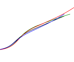
Numerical simulations were conducted for values of the Reynolds number between $10^4$ and $10^6$ and for values of the Froude number between $0.1$ and $0.8$. The case $Re=10^5$ and $F=0.5$ is presented in figure 3 where the black curve is $\varphi /\varphi _{max}$ and the red curve is $\delta /h_n$ calculated from (6.5), both given as a function of the normalized abscissa along the channel $x/h_n$ counted from the entrance. The slope corresponding to these values of the Reynolds and Froude numbers is $\sin \theta =1/2162\simeq 4.6\times 10^{-4}$ (note that $\mathrm {tg} \theta$ is practically equal to $\sin \theta$). In this case, the length of the flow developing zone is $L/h_n=81.7$ (marked on figure 3 with a dashed line).

Figure 3. Variations of the normalized enstrophy $\varphi / \varphi _{{max}}$ (black curve) and of the normalized boundary layer thickness $\delta /h_n$ (red curve) according to law (6.5) with the normalized abscissa along the channel $x/h_n$, in the case $Re=10^5$ and $F=0.5$.

The calculated values of $L/h_n$ for all studied cases are gathered in figure 4(a) for different values of the Froude number. The different symbols and colours correspond to: $Re=10^4$ (black $\bullet$); $Re=5\times 10^4$ (blue $\blacksquare$); $Re=10^5$ (green $\blacklozenge$); $Re=5\times 10^5$ (red $\blacktriangle$) and $Re=10^6$ (black $\blacktriangledown$). The value of $L/h_n$ depends mainly on the Reynolds number but weakly on the Froude number. For a given value of $Re$, it is larger when $F$ becomes close to 1 and slightly larger for very small values of $F$. For a given value of the Froude number, $L/h_n$ increases with the value of $Re$. The variation of $L/h_n$ with the Reynolds number for a Froude number equal to $0.5$ is shown in figure 4(b) in a logarithmic plot. In the case $F=0.5$, it is very close to the law $L/h_n\simeq 25.8 Re^{1/10}$ (dashed line).

Figure 4. (a) Variation of the ratio of the length of the flow developing zone $L$ over the normal depth $h_n$ with the Froude number: $Re=10^4$ (black $\bullet$); $Re=5\times 10^4$ (blue $\blacksquare$); $Re=10^5$ (green $\blacklozenge$); $Re=5 \times 10^5$ (red $\blacktriangle$); $Re=10^6$ (black $\blacktriangledown$). (b) Variations of $L/h_n$ with the Reynolds number for $F=0.5$ (dots); dashed line: $L/h_n=25.8Re^{1/10}$.

It is very difficult to make comparisons with experimental results due to the fact that the length of the flow developing zone is defined differently, that only relatively small values of the Reynolds number can be studied in laboratory channels and that the channels used in the experiments have a finite width. The goal here is only to check that the order of magnitude of the calculated length $L$ is reasonable.

Kırkgöz & Ardıçhoğlu (1997) conducted experiments in a smooth channel $0.3\ \mathrm {m}$ wide. Due to the relatively small value of the channel width, many experiments are in fact 2-D situations and cannot be considered for a comparison with a 1-D model (the ratio width/depth is as low as $1.50$ in an experiment). Therefore, only the cases where the ratio width over depth is larger than 4 are considered thereafter (and a ratio of 4 is already quite small). The remaining measurements have values of the Reynolds numbers between $7\times 10^3$ and $2.1 \times 10^4$ and values of the Froude number between $0.30$ and $0.72$. The authors presented the values of $L/h$ as a function of the ratio $4Re/F$ (or $Re_H/F$, where $Re_H=4Re$) and proposed the empirical law $L/h=76-0.0001(4Re/F)$. We can remark that this law gives obviously wrong results if the Reynolds number is high enough since the predicted value of $L/h$ becomes negative. For values of the Froude number equal to $0.1$, $0.5$ and $0.8$, $L/h$ becomes negative if $Re$ is higher than $19\ 000$, $95\ 000$ and $152\ 000$, respectively. Furthermore, the lowest measured values of $L/h$ were found in the cases of narrow channels (when the ratio width/depth is smaller than 4).

The calculated values of $L/h_n$ as a function of $4Re/F$ are presented in figure 5 (red $\bullet$) together with the measured values of Kırkgöz & Ardıçhoğlu (1997) (black $\blacktriangle$) and the values calculated from their empirical law (blue $\blacksquare$). The range of the Reynolds and Froude numbers was restricted to the range of the experiments with the largest width/depth ratios (i.e. $Re=10^4$ and $0.25\leqslant F\leqslant 0.8$) In spite of all above reservations about this comparison, the order of magnitude of the length of the flow developing zone seems reasonable for these values of the Reynolds and Froude numbers.

Figure 5. Ratio of the length of the flow developing zone over the normal depth $L/h_n$ as a function of $4Re/F$: calculated with the model (red $\bullet$); measured values of Kırkgöz & Ardıçhoğlu (1997) (black $\blacktriangle$); values calculated with the empirical law of Kırkgöz & Ardıçhoğlu (1997) (blue $\blacksquare$).

6.3. Unsteady flows

The numerical simulations of unsteady flows are inspired by the experiments of Nezu et al. (1997). The discharge $q_0$ prescribed at the entrance of the channel is sinusoidal for half a period to take into account one rising stage followed by one falling stage, after a delay time $t_R$ large enough for the base flow to be in steady-state conditions. At time $t_R$ the discharge is increased from a base value $q_b$ to a peak value $q_p$ after a time $T_d$, then decreased to the base value $q_b$ after the same duration. Therefore, $q_0=q_b$ if $t\leqslant t_R$ or if $t\geqslant t_R+2T_d$. Otherwise, $q_0$ is given by

(6.6)\begin{equation} q_0=q_b + \frac{q_p-q_b}{2}\left[1-\cos \frac{{\rm \pi} (t-t_R)}{T_d}\right] \quad \mathrm{if} \ t_R \leqslant t \leqslant t_R+2T_d.\end{equation}

The flow is supposed to be non-developed at the beginning of the channel. This means that $\varphi =0$ is prescribed at the entrance. The flow is studied far enough from the entrance, at an abscissa $x$, for the flow to be fully developed ($x>L$). Simulations were performed for values of the Reynolds number equal to $10^4$, $10^5$ and $10^6$, values of the Froude number equal to $0.18$, $0.5$ and $0.8$, and values of $T_d$ equal to $30\ \mathrm {s}$ (a strongly unsteady case), $120 \ \mathrm {s}$ and $240\ \mathrm {s}$. In addition, the ratio $q_p/q_b$ was set to 4 for $Re=10^4$ and to 5 otherwise and various channel lengths $\ell$ were considered. The base flow is in the normal conditions and this prescribes the value of $\sin \theta$. The various parameters of the simulations are gathered in table 1.

Table 1. Parameters used for the numerical simulations in the unsteady case.

The variation of the depth $h$ against the average velocity $U$ shows the characteristic loop diagram observed for rivers in flood, which are simulated with the rising and falling discharge implied by (6.6). The peak velocity appears before the peak depth. The cases C7M24 (low Froude number $F=0.18$, weakly unsteady $T_d=240\ \mathrm {s}$, black curve), C7M30 (low Froude number $F=0.18$, strongly unsteady $T_d=30\ \mathrm {s}$, blue curve) and C4M24 (larger Froude number $F=0.8$, weakly unsteady $T_d=240\ \mathrm {s}$, red curve) are presented in figure 6(a) with $Re=10^5$ (see table 1) where the loops are run counterclockwise. The loop is wider if the flow is more strongly unsteady (C7M30) or if the Froude number increases (C4M24). The evolutions of the depth (black curve), the average velocity (red curve) and the enstrophy (blue curve) are presented in figures 6(b) (C7M24), 6(c) (C4M24) and 6(d) (C7M30). Weakly unsteady cases (figures 6(b) and 6(c) are closer to a kinematic wave with only slight shape changes during the propagation, whereas, in a strongly unsteady case (figure 6(d), the front of the wave steepens with a tendency to take a sawtooth shape. The evolution of the enstrophy depends on the case: for a small Froude number, the enstrophy increases in the wave (figures 6b and 6d) while it decreases for a larger Froude number (figure 6c). For intermediate values of the Froude number, the enstrophy increases in the early stages of the wave and then decreases (figure 7(a) for $F=0.5$).

Figure 6. (a) Normalized depth $h/h_{{max}}$ as a function of the normalized velocity $U/U_{{max}}$: cases C7M24 (black curve), C7M30 (blue curve) and C4M24 (red curve) (see table 1). (b–d) Evolution of the depth (black curve), velocity (red curve) and enstrophy (blue curve) normalized by their value for the normal flow as a function of normalized time: cases C7M24 (b), C4M24 (c) and C7M30 (d).

Figure 7. (a) Comparison between the cases C3S30 (solid curves) and C3M30 (dashed curves): depth (black curves), velocity (red curves) and enstrophy (blue curves) normalized by their normal value as a function of normalized time. (b) Reconstruction of the bottom shear stress normalized by its value in the base flow (solid curves) for the cases C7M24 (black), C7M30 (blue) and C4M24 (red); dashed curves: normalized depth (same colours).

The influence of the downstream boundary condition can be important in some cases, particularly during the falling stage of the wave, as there is some reflection on the weir. This phenomenon can lead to a complex behaviour at the end of the falling stage or shortly after that as in the C7M30 case (figure 6d). The abscissa $x$ considered to study the flow was usually chosen far from the weir (which is at an abscissa $\ell$), but the effects of the interactions with the weir are not trivial as it can be seen from the comparison in figure 7(a) between the cases C3S30 ($x=17\ \mathrm {m}$ and $\ell = 20\ \mathrm {m}$, solid curves) and C3M30 ($x=17\ \mathrm {m}$ and $\ell = 30\ \mathrm {m}$, dashed curves), where in both cases $Re=10^5$ and $F=0.5$. The graphs of $h/h_n$ (black curves), $U/U_n$ (red curves) and $\varphi /\varphi _n$ (blue curves) show that the end of the falling stage is more complex when the distance to the weir is larger. Even the amplitude of the wave is modified by the distance to the weir. Because of this sensitivity to the downstream boundary condition, it is not possible to make precise comparisons to experimental results without a precise knowledge of the weir used at the end of the channel and, more generally, of the precise hydraulic conditions of the experiments, such as the slope.

The reconstruction of the bottom shear stress with the expression (5.1) is presented in figure 7(b) for the cases C7M24 (black curves), C7M30 (blue curves) and C4M24 (red curves). The solid curves show the ratios of $\tau _{sh}(0)$, denoted by $\tau _b$, over its value for the base flow, denoted by $\tau _{bn}$, and the dashed curves show the ratios of $h/h_n$. As for the average velocity, the peak value of the bottom shear stress is attained before the peak depth. This is in accordance with the results of Nezu et al. (1997). The difference between these two peaks increases for a strongly unsteady case or for a larger Froude number. In a strongly unsteady case (C7M30), the graph of the bottom shear stress approaches a sawtooth shape and the end of the falling stage is complex due to reflections on the weir.

The reconstruction of the velocity profile is presented in figure 8(a) for the C7M24 case and in figure 8(b) for the C7M30 case, with $u^{+}=u/u_b$, $z^{+}=zu_b/\nu$, $u_b$ being the friction velocity calculated with (5.1) and $u_b=\sqrt {\tau _b / \rho }$. Even in the case of a relatively weak unsteadiness (C7M24), the velocity profile during the wave is modified with respect to the velocity profile of the steady case (black curve) both in the inner layer and in the outer layer. The red curve shows the velocity profile at the peak depth. In a strongly unsteady case (C7M30), the evolution of the velocity profile is more complex. The black curve is the profile of the steady flow and the green, red and blue curves are the profiles during the early part of the rising stage, at the peak depth and at the end of the falling stage, respectively.

Figure 8. Reconstruction of the velocity profile. (a) Case C7M24: steady profile (black) and profile at the peak depth (red); (b) Case C7M30: steady profile (black) and profiles at the early part of the rising stage (green), at the peak depth (red) and at the end of the falling stage (blue).

These curves can be approximately interpreted with the same laws as in the steady case but the constants have apparent values that are different from the steady-case values. In the outer layer a log law is approximately satisfied with an apparent von Kármán constant $\kappa _{{app}}$ and an apparent integration constant $B_{{app}}$. Furthermore, in many cases, a deviation from this apparent log law can be interpreted as a wake function, as in Coles (1956), with an apparent wake-strength parameter $\varPi _{{app}}$. The velocity profiles can be approximately described in the outer layer with the law

(6.7)\begin{equation} u^{+}=\frac{1}{\kappa_{{app}}}\ln z^{+}+B_{{app}}+\frac{2\varPi_{{app}}}{\kappa_{{app}}}\sin^2\frac{{\rm \pi} z}{2h}. \end{equation}

Note that this relation is only a convenient description of the actual velocity profile in the outer layer, which is in fact given by (5.3). This relation and, in particular, the wake function, are only a rough approximation of the real function calculated by the model. It is mainly useful for comparisons with laws given in the literature in the case of unsteady flows.

The variations of the apparent von Kármán constant are presented in figure 9(a) for the weakly unsteady cases ($T_d=240\ \mathrm {s}$) C7M24 ($F=0.18$, black $\blacklozenge$), C3M24 ($F=0.5$, blue $\blacksquare$) and C4M24 ($F=0.8$, red $\bullet$), and in figure 9(b) for the strongly unsteady cases ($T_d=30\ \mathrm {s}$) C7M30 ($F=0.18$, black $\blacklozenge$), C3M30 ($F=0.5$, blue $\blacksquare$) and C4M30 ($F=0.8$, red $\bullet$). For $F=0.8$, the value of the apparent von Kármán constant remains close to the value $\kappa =0.41$ but, for smaller Froude numbers, the difference between $\kappa _{{app}}$ and $\kappa$ can be important. For the weakly unsteady cases, the overall evolution is that $\kappa _{{app}}$ increases in the rising stage, reaching a value $\kappa _{{app}} \simeq 0.435$ for $F=0.18$, and decreases in the falling stage. For the strongly unsteady cases, the evolution of $\kappa _{{app}}$ is more complex, especially because the interaction with the weir can have a strong effect at the end of the falling stage. The value of $\kappa _{{app}}$ increases at the beginning of the rising stage, reaching $\kappa _{{app}} \simeq 0.46$ for $F=0.18$, and decreases before the peak depth and becomes negative at the end of the falling stage.

Figure 9. Apparent von Kármán constant (a,b), apparent integration constant (c,d) and apparent wake-strength parameter (e, f) as a function of normalized time. (a,c,e) Cases C7M24 (black $\blacklozenge$), C3M24 (blue $\blacksquare$) and C4M24 (red $\bullet$); (b,d, f) Cases C7M30 (black $\blacklozenge$), C3M30 (blue $\blacksquare$) and C4M30 (red $\bullet$).

The variations of the apparent integration constant $B_{{app}}$ are similar. They are presented in figure 9(c) for the cases C7M24 (black $\blacklozenge$), C3M24 (blue $\blacksquare$) and C4M24 (red $\bullet$), and in figure 9(d) for the cases C7M30 (black $\blacklozenge$), C3M30 (blue $\blacksquare$) and C4M30 (red $\bullet$). From the steady value $B=5.28$, $B_{{app}}$ increases and can become larger than 7 for $F=0.18$. At the end of the falling stage, $B_{{app}}$ becomes negative in some cases. The difference between $B_{{app}}$ and $B$ is not small, even for $F=0.8$.

The apparent wake-strength parameter $\varPi _{{app}}$ is shown in figure 9(e) for the cases C7M24 (black $\blacklozenge$), C3M24 (blue $\blacksquare$) and C4M24 (red $\bullet$), and in figure 9( f) for the cases C7M30 (black $\blacklozenge$), C3M30 (blue $\blacksquare$) and C4M30 (red $\bullet$). Its value remains close to 0 for $F=0.8$ but is larger for smaller Froude numbers, particularly for $F=0.18$ where it reaches a maximum of $\varPi _{{app}}\simeq 0.10$ for $T_d=240\ \mathrm {s}$ and $\varPi _{{app}}\simeq 0.4$ for $T_d=30\ \mathrm {s}$. In most cases, $\varPi _{{app}}$ is positive but it can take negative values at the beginning of the rising stage for $F=0.18$ and $T_d=30\ \mathrm {s}$ or at the end of the falling stage in some cases.

The graphs of figure 9 show that the constants of the apparent law (6.7) depend strongly on the Froude number. On the contrary, simulations performed for $Re=10^4$, $Re=10^5$ and $Re=10^6$ at a given Froude number show that these apparent constants depend weakly on the Reynolds number.

In the viscous sublayer the expression (5.8) can be used to reconstruct the velocity profile. The ratio $u^{+}/z^{+}$ is calculated with this expression and the results are presented in figure 10 for the cases C7M24 (black $\blacksquare$), C7M30 (blue $\blacksquare$) and C4M24 (red $\blacksquare$). In the steady state $u^{+}/z^{+}=1$ but, for unsteady flows, this ratio is smaller. For $F=0.8$, $u^{+}/z^{+}$ remains close to 1 but, for $F=0.18$, $u^{+}/z^{+}$ decreases below $0.8$. For the weakly unsteady case ($T_d=240\ \mathrm {s}$), this ratio decreases in the rising stage and increases in the falling stage, but in the strongly unsteady case ($T_d=30\ \mathrm {s}$), the minimum value of $u^{+}/z^{+}$ is reached before the peak depth and there is some further perturbations at the end of the falling stage due to interactions with the weir.

Figure 10. Ratio $u^{+}/z^{+}$ as a function of normalized time for the cases C7M24 (black $\blacksquare$), C7M30 (blue $\blacksquare$) and C4M24 (red $\blacksquare$).

The calculation of the von Kármán constant by Onitsuka & Nezu (2000) and Nezu & Onitsuka (2002) in unsteady flows used an evaluation of the friction velocity assuming the validity in unsteady situations of the law $u^{+}=z^{+}$ in the viscous sublayer. One of the results of the present work is that this law is not valid in an unsteady case where $u^{+}$ is still a linear function of $z^{+}$ but with $u^{+}/z^{+}<1$. As seen in figure 10, the difference can be important, particularly for low Froude numbers, with values of $u^{+}/z^{+}$ as small as $0.7$. Consequently, using the relation $u^{+}=z^{+}$ in the viscous sublayer to evaluate the friction velocity in unsteady situations can entail a large error in the calculation of the apparent von Kármán constant and also in the apparent integration constant.

We have calculated the apparent von Kármán constant by using $u^{+}=z^{+}$ to calculate the friction velocity instead of using the relation (5.1) in order to replicate the calculation of Onitsuka & Nezu (2000) and Nezu & Onitsuka (2002). Deliberately using this wrong value of the friction velocity gives entirely different values of the apparent von Kármán constant. The results are presented in figure 11(a) for the case C7M24 and in figure 11(b) for the case C7M30, where the values of $\kappa _{{app}}$ calculated by this method (red $\blacksquare$) are compared with the normal calculation (black $\bullet$) that uses the friction velocity predicted by the model. When $u^{+}=z^{+}$ is used, $\kappa _{{app}}$ decreases in the rising stage instead of increasing and then increases during the falling stage or, for a strongly unsteady case, before the end of the rising stage. This evolution is rather close to the results of Nezu & Onitsuka (2002). There is also, particularly for a strongly unsteady case, a sudden increase of $\kappa _{{app}}$ near the beginning of the rising stage before a rapid decrease, and this feature was noted by Onitsuka & Nezu (2000). Because of the similarity between our calculations of $\kappa _{{app}}$ using $u^{+}=z^{+}$ in the viscous sublayer, even if this relation is not valid in our approach, and the results of Onitsuka & Nezu (2000) and Nezu & Onitsuka (2002), we think that the qualitative discrepancies between our really predicted values of $\kappa _{{app}}$ (figures 9a and 9b) and the calculations made from experimental results in the literature are due to the wrong assumption that $u^{+}=z^{+}$ is valid in unsteady situations, which leads to large errors in the evaluation of $\kappa _{{app}}$. The evaluation of the apparent integration constant is also flawed if the validity of $u^{+}=z^{+}$ is assumed in unsteady flows.

Figure 11. Comparison of the apparent von Kármán constant calculated with the friction velocity obtained with (5.1) (black) or by assuming that $u^{+}=z^{+}$ (red): (a) case C7M24; (b) case C7M30.

6.4. Comparisons with experiments in 1-D unsteady open-channel flows

6.4.1. Test case 1: experiment SC3T1 of Nezu et al. (1997)

To assess the validity of the model, it is necessary to compare with experiments made in an unsteady and variable case since the model introduces the first-order corrections, which are equal to zero in a stationary and uniform flow. The experiments of Nezu & Nakagawa (1995) and Nezu et al. (1997) were conducted in a 10 m long and 40 cm wide channel where the discharge was controlled in order to produce a flood flow. Starting from a base flow of depth $h_b$, the discharge was increased and then decreased with a peak depth $h_p$. The hydrograph was a sine curve. The duration from the base discharge to the peak discharge was $T_d$. Detailed information on the experiments and measurements are available in Nezu & Nakagawa (1995) and Nezu et al. (1997). In our model, the Reynolds number is assumed to be very large since $\eta =1/(\kappa ^2Re)$ is supposed to be of $O(\varepsilon ^{2+m})$ with $m>0$. The hydraulic conditions of these experiments are at the lower limit of validity since the Reynolds number is only of the order of $10^4$. This order of magnitude is typical of laboratory conditions but natural flows have usually much higher values of the Reynolds number, typically around $10^5$ or $10^6$, which are more suited to our model.

We simulated the experiment SC3T1 where $T_d=60\ \mathrm {s}$ and $h_b=4.05\ \mathrm {cm}$. Since the flow is subcritical, it is controlled by the downstream boundary condition. The authors gave no information on their downstream control, but it is likely that it was a weir of some sort. As above, we used a formula used for sharp-crested weirs,

(6.8)\begin{equation} q_{N+1}=\frac{2}{3}\left(C_1+C_2\frac{h_N-d}{d}\right) \sqrt{2g(h_N-d)^3}, \end{equation}

to calculate the discharge $q=hU$ at cell $N+1$ from the depth $h$ at cell $N$. In this expression d is the weir height. We tuned the coefficients $C_1$ and $C_2$ to obtain the values at the peak flow. Some hydraulic conditions were not given by the authors and some conjectures were necessary to obtain some parameters of the calculation. Neither the mean velocity $U_b$ of the base flow nor the Reynolds number of the base flow were given. From the values of the von Kármán constant $\kappa$, the integration constant $B$, the wake-strength parameter $\varPi$ and the value of the friction velocity $v_b$ for the base flow, the average velocity of the base flow was estimated by an integration over the depth of the law (1.2). The viscosity is not given either, nor the temperature. With the values of $\kappa$, $B$, $\varPi$ and $v_b$ for the peak flow, the peak mean velocity $U_p$ was estimated. The Reynolds number of the peak flow was provided, which allowed us to estimate the kinematic viscosity $\nu$.

The friction coefficient $C_f$ was calculated with the explicit relation (4.21). The base flow is supposed to be a steady and uniform flow. However, it was not possible to obtain a stationary and uniform flow with the value $1/600$ given for the slope. This would imply a friction coefficient roughly twice as large as what can be calculated with classical relations used in hydraulics, even considering the hydraulic radius instead of the depth in the definition of the Reynolds number. Since no value of the friction coefficient and no discussion about this coefficient are given by the authors, we assumed that it was a 2-D effect due to the lateral walls or some other unspecified condition. To obtain a uniform base flow, we had to use a smaller slope of $1/1456$.

In a first scenario, we chose the coefficients $C_1$ and $C_2$ to have a uniform base flow of depth $h_b$, mean velocity $U_b$ and also the same value of $h_p$ as in the experiments, and the same value of $U_p$ at the peak flow as it can be deduced from the integration of (1.2) over the depth with the parameters $\kappa =0.41$, $B=3.44$ and $\varPi =0.33$ found by Nezu et al. (1997). However, it appears that the model underestimated the velocity in the defect layer. Nezu et al. (1997) found a value $\varPi =0.33$ of the wake-strength parameter at the peak flow whereas the model finds an apparent wake-strength parameter of only $\varPi _{{app}} \simeq 0.02$. Because the average velocities were assumed to be equal, the velocity was overestimated in the ‘log layer’ as a result. As the velocity profile in this layer was only shifted vertically by a constant value, it seemed more logical to use a second scenario where the downstream boundary condition was chosen to obtain the same mean velocity in the ‘log layer’.

The final set of parameters used for the calculations in this second scenario was: $\nu = 8.68 \times 10^{-7} \ \mathrm {m}^2\ \mathrm {s}^{-1}$ (which corresponds to a temperature of $26.3\,^{\circ }\mathrm {C}$), $C_1=0.61$, $C_2=0.0305$, $d=7.9\ \mathrm {mm}$, $U_b=0.316 \ \mathrm {m}\ \mathrm {s}^{-1}$, $\kappa =0.41$, $R=2.67$, $g=9.8\ \mathrm {m}\ \mathrm {s}^{-2}$. The friction coefficient, calculated with (4.21), was equal to 0.00275 in the base flow and decreased during the flood event. The various quantities were taken at a distance of $7\ \mathrm {m}$ from the beginning of the channel, as in the experiments. The peak depth was $h_p=6.6\ \mathrm {cm}$ and the average velocity at the peak depth was $U_p=0.513\ \mathrm {m}\ \mathrm {s}^{-1}$. However, since the peak velocity is reached before the peak depth, this was not the maximum velocity, which was $U_{{max}}=0.517\ \mathrm {m}\ \mathrm {s}^{-1}$. The peak value of the Reynolds number was $Re_p=3.9 \times 10^4$, as in the experiments.

The velocity profile was reconstructed for the base flow and at the peak depth ($h=h_p$). The results are presented in figures 12(a) and 12(b), respectively. The experimental measures were presented with the inner variables $u^+$ and $z^+$ in Nezu et al. (1997) (where our $z$ is denoted by $y$). Using the value of the friction velocity used by the authors and the kinematic viscosity conjectured as explained above, we reconstructed the experimental dimensional velocity profile (black dots in figure 12). Nezu et al. (1997) calculated the friction velocity for the SC3T1 case assuming the validity of the log law $u^+ =(1/\kappa )\ln z^+ +B$ with $\kappa =0.41$. With this method, they found a friction velocity of $1.63\ \mathrm {cm}\ \mathrm {s}^{-1}$ for the base flow and $2.66\ \mathrm {cm}\ \mathrm {s}^{-1}$ for the peak flow. Then the integration constant and the wake-strength parameter were found to fit the measures. The curves obtained with the law (1.2) are shown in black in figure 12 together with the law $u^+=z^+$ used in the viscous sublayer. We did not reproduce the correction due to the Van Driest damping function that would smooth the transition from one law to the other. For the base flow, the standard value $B=5.3$ was found. For the peak flow, they obtained the value $B=3.44$ for the integration constant. In addition, Nezu et al. (1997) used a wake-strength parameter $\varPi =0.16$ for the base flow and $\varPi =0.33$ for the peak flow. Such a deviation from the log law is clear at the peak depth (see figure 12b) but it is not so obvious for the base flow (figure 12a).

Figure 12. Reconstructed velocity profile (red curve) and comparisons with the experimental measures of Nezu et al. (1997) (black dots) and with the law (1.2) proposed by Nezu et al. (1997) to fit their measures (black curve). (a) Base flow; (b) peak flow.

The reconstruction of the velocity profile with the model is presented in figure 12 with a red curve. The relations (5.3) and (5.4) were used for the outer and inner layers, respectively, with good matching. The agreement with the experimental measures is very good for the base flow (figure 12a) in spite of the absence of a wake function. At the peak flow, there is a discrepancy between the predictions of the model and the experimental results in the defect layer. The apparent wake-strength parameter is underestimated since we found that $\varPi _{{app}}=0.02$, which is much smaller than the value $\varPi =0.33$ found by Nezu et al. (1997). The origin of this deviation in open channels is not always clear and could be caused by 2-D effects. Below the defect layer, the agreement is very good. The law (5.3) in the outer layer is presented, without the matching with the law of the inner layer, in figure 13(a). The comparison with the experimental measures (black dots) shows that the slope of the curve found with the model agrees slightly better in the ‘log-law region’ than the law used by Nezu et al. (1997) (black curve). We use the term ‘log-law region’ although the profile in this region does not satisfy a pure log law according to our model.

Figure 13. (a) Comparison of the reconstructed velocity profile in the outer layer (red curve) with the experimental measures of Nezu et al. (1997) (black dots) and the fitting law proposed by Nezu et al. (1997) (black curve). (b) Bottom shear stress normalized by its time-averaged value calculated by the model (red curve) superimposed over the curves calculated by Nezu et al. (1997) assuming the validity of the log law with $\kappa =0.41$. Variations of the flow depth during the same flood event expressed as ${\rm \Delta} h = h-h_b$ normalized by $h_p-h_b$ (blue curve) superimposed over the measures of Nezu et al. (1997).

The bottom shear stress was reconstructed with the relation (5.1). It is presented during the whole flood event in figure 13(b) (red curve). The curve is superimposed over the results of Nezu et al. (1997) where the bottom shear stress (denoted here by $\tau _w$) is first calculated by the log law with the assumption $\kappa =0.41$ and then normalized by the time-averaged value $\bar {\tau }_w$. The results corresponding to the SC3T1 case is the case $\alpha =0.95 \times 10^{-3}$ ($\alpha$ is an unsteadiness parameter defined in Nezu et al. 1997). The duration used to calculate the time-averaged value is not specified. We assumed it was the duration $2T_d$ of the flood event. The value of the bottom shear stress presented by Nezu et al. (1997) is thus not a measure but results from an assumption. In our model, this assumption is not exactly satisfied since there is a small deviation to the log law due to the first-order correction. Moreover, the apparent von Kármán constant $\kappa _{{app}} = 0.414$ is slightly different from the standard value $0.41$. This entails a small difference in the friction velocity. We found the value $v_b = 2.45\ \mathrm {cm}\ \mathrm {s}^{-1}$ at the peak depth instead of the value $v_b = 2.66\ \mathrm {cm}\ \mathrm {s}^{-1}$ found by Nezu et al. (1997). There is thus also a small difference on the bottom shear stress. The curve $\alpha =0.95 \times 10^{-3}$ is not always distinguishable but it is the second highest curve after the case $\alpha =1.28 \times 10^{-3}$. The curve found with the model (red) is slightly smaller than the curve (black) of Nezu et al. (1997), but both curves are very close. It can be noted that in both cases, the maximum value of the bottom shear stress is reached before the maximum value of the depth. The variation of the depth is presented with the quantity ${\rm \Delta} h = h-h_b$ normalized by ${\rm \Delta} h_p = h_p - h_b$, in blue for our model, superimposed with the black curve of Nezu et al. (1997). Both curves are very close to one another. The depth variation is a consequence of the hydrograph, which was exactly a sine curve in our simulation. In the experiments it was also a sine curve with good accuracy. The small differences are probably not significant.

6.4.2. Test case 2: experiment U2 of Onitsuka & Nezu (2000)

The second test case is the case U2 of Onitsuka & Nezu (2000). The experiment is similar to the first test case except that the measurements are made at a distance of $8\ \mathrm {m}$ from the channel entrance and that $T_d = 120 \ \mathrm {s}$. The hydrograph, the slope and the viscosity are not specified. We assumed that the hydrograph was a sine function as in the first test case. We chose the slope in order to have a uniform base flow. This gives $\sin \theta =8.25 \times 10^{-6}$. The kinematic viscosity was calculated from the values of the base depth $h_b=6.0\ \mathrm {cm}$, the base mean velocity $U_b=3.33 \ \mathrm {cm}\ \mathrm {s}^{-1}$ and the Reynolds number of the base flow $Re_b =2.32 \times 10^3$ ($Re=hU/\nu$). This Reynolds number is very small and below the validity domain of the matching procedure and of the viscous scaling, which necessitates $Re=O(\varepsilon ^{-2-m})$ with $m>0$. The slope is also too small for the model, which is not valid if the slope is equal to zero. The Froude number of the base flow was also very small: $F_b = 0.04$. As a rule, the model is valid if $Re>10^4$ and $\sin \theta > 10^{-4}$. Below these values, the matching procedure and the viscous scaling are not accurate since some neglected terms are not negligible. This implies that the velocity profile in the inner layer is not accurate. However, the predictions of the model in the outer layer are very good.

The friction coefficient was calculated with the explicit relation (4.21) with $\kappa =0.41$ and $R=2.67$. For the base flow, the friction coefficient was $C_{f\! b} = 0.00438$ and decreased when the depth increased. The flow is subcritical and is controlled by the downstream boundary condition. We used the same boundary condition as in the first test case, with $C_1=0.70$, $C_2=0.08$ and $d=5.04\ \mathrm {cm}$. These values were chosen to reach the same peak values as in the experiment. The peak Reynolds number, depth and average velocity were respectively $Re_p=1.16 \times 10^4$, $h_p=7.8 \ \mathrm {cm}$ and $U_p = 12.8 \ \mathrm {cm}\ \mathrm {s}^{-1}$.

The velocity profile in the outer layer of the base flow is accurately reconstructed from the model. The reconstruction of the velocity profile at the peak depth is presented in figure 14 in the outer layer (from a depth corresponding to $z^+=30$ in the inner variables until the free surface). The experimental measurements were accurately fitted by Onitsuka & Nezu (2000) with the law expressed with the inner variables $u^+ = (1/\kappa )\ln z^+ + B$, assuming the validity of the law $u^+ = z^+$ in the viscous sublayer to calculate the friction velocity. Using the value of the friction velocity given by the authors ($v_b = 0.65 \ \mathrm {cm}\ \mathrm {s}^{-1}$ for the peak flow), we followed the reverse path to obtain the experimental dimensional velocity profile (black line in figure 14). The solid red curve is the velocity profile reconstructed from the model with the relation (5.3). The agreement with the experimental curve is very good. Contrary to the first test case, no wake-strength parameter was found by Onitsuka & Nezu (2000) whereas the reconstructed velocity profile shows a small non-zero value of $\varPi _{{app}}$. As mentioned above, the existence or absence of a ‘wake function’ in the case of open-channel flows is not well understood and could be caused by several effects related to secondary currents or to the flow history.

Figure 14. Velocity profile in the outer layer calculated with the model for the simulation of the experiment U2 of Onitsuka & Nezu (2000) (red curve) and comparison with the law obtained by Onitsuka & Nezu (2000) to fit their measures (black curve).

6.4.3. Test case 3: experiment N30 of Nezu & Onitsuka (2002)

The third test case is the case N30 of Nezu & Onitsuka (2002). It is similar to the second test case except that $T_d = 30 \ \mathrm {s}$, $h_b=6\ \mathrm {cm}$, $U_b=5.2 \ \mathrm {cm}\ \mathrm {s}^{-1}$ and $Re_b = 2.5 \times 10^3$. The slope is calculated assuming the base flow is uniform. This leads to the value $\sin \theta =1.97 \times 10^{-5}$. As in § 6.4.2, the Reynolds number and the slope are very small which implies that the matching and the profile in the inner layer are not accurate. On the other hand, the shallow-water scaling is still valid and the velocity profile in the outer layer is accurate.

The parameters used for the simulation are $C_1 =0.60$, $C_2=0.03$, $d=4.556 \ \mathrm {cm}$ (with the same downstream boundary condition as above), $h_p=7.9 \ \mathrm {cm}$ and $U_p=14.2 \ \mathrm {cm}\ \mathrm {s}^{-1}$ (at the peak depth). The friction coefficient was calculated with the explicit relation (4.21), $\kappa =0.41$ and $R=2.67$. It is not clear whether the values at $t/T_d=1.0$ were measured at the peak depth or at the peak velocity, which is reached a little bit earlier. Since the average velocity found from the integration over the depth of the fitting law given by the authors with the values $\kappa =0.347$ and $B=3.48$ obtained at $t/T_d=1.0$ (Nezu & Onitsuka 2001, 2002) gives the maximum velocity $U_{{max}}=14.6\ \mathrm {cm}\ \mathrm {s}^{-1}$, we assumed that it was the peak velocity, where $h=7.78\ \mathrm {cm}$.

The comparison of the velocity profile reconstructed in the outer layer using the relation (5.3) (red curve) with the experimental results of Nezu & Onitsuka (2002) (black dots) is presented in figure 15. The experimental results are given in Nezu & Onitsuka in the inner variables $u^+$ and $z^+$. They were converted in dimensional form using the value of the friction velocity ($v_b=0.79\ \mathrm {cm}\ \mathrm {s}^{-1}$ at the peak flow). The log law proposed by the authors to fit the experimental results is shown in the figure (black line). The figure shows the velocity profile in the outer layer from a value of $z$ corresponding to $z^+=50$ until the free surface. The velocity profile found from the model is in good agreement with the experimental profile in the outer layer.

Figure 15. Velocity profile reconstructed from the model for the experiment N30 of Nezu & Onitsuka (2002) (red curve) and comparison with the experimental measures (black dots) and the fitting curve of Nezu & Onitsuka (2002) (black curve).

6.5. Numerical scheme for the 2-D model

In the 2-D case the shape of the cross-section must be taken into account. This implies defining the distance $z_b$ between the bed and the sloping plane $Oxy$ (see figure 1). This distance $z_b$ defines a bathymetry and can depend on $x$ or $y$. We assume that the variations of $z_b$ with $x$ or $y$ are very small such that $\Vert \textbf {grad}\, z_b\Vert /\Vert \textbf {grad}\, h \Vert =O(\varepsilon )$. In this case, the asymptotic expansions are exactly the same as above and the only difference is the presence of a term in $\textbf {grad}\, z_b$ in the depth-averaged momentum equation. The hyperbolic system with source terms of (4.26)–(4.28) can thus be written as

(6.9)\begin{equation} {\frac{\partial\boldsymbol{\mathcal{U}}}{\partial t}+{\textbf{div} }\,(\boldsymbol{\mathcal{F} })=\boldsymbol{\mathcal{S}}(\boldsymbol{\mathcal{U}})},\end{equation}

where

(6.10a,b) \begin{equation} {\boldsymbol{\mathcal{U}}=(h,h\boldsymbol{U},h \boldsymbol{\varphi})^{\mathrm T}},\quad {\boldsymbol{\mathcal{F}}=\left(h\boldsymbol{U},h \boldsymbol{U}\otimes\boldsymbol{U}+\frac{gh^{2}}{2}\cos\theta {\boldsymbol{\mathsf{I}}}+h^{3}\boldsymbol{\varphi},h\boldsymbol{\varphi} \otimes\boldsymbol{U}\right)^{\mathrm T}}, \end{equation}

and $\boldsymbol {\mathcal {S}} (\boldsymbol {\mathcal {U}})=(S_1, \boldsymbol {S_2}, {\boldsymbol{\mathsf{S}}}_{\boldsymbol 3})$ with $S_1=0$,

(6.11)\begin{align} \boldsymbol{S_2}&={-}gh\, \mathbf{grad}\, z_{b}+ \left(1-\frac{\alpha_{1}}{\kappa}\sqrt{C_{f}}\right) (\hat{\boldsymbol{g}}h-C_{f}\boldsymbol{U} \Vert \boldsymbol{U}\Vert )\nonumber\\ &\quad +\alpha(\kappa-\alpha_{1}\sqrt{C_{f}}) \sqrt{C_{f}}h\left(h\, \mathrm{tr}\, \boldsymbol{\varphi}- \frac{\hat{g}}{\kappa^{2}}\right)\frac{\hat{\boldsymbol{g}}}{\hat{g}} -\alpha_{1}\kappa\sqrt{C_{f}}h\left(h\boldsymbol{\varphi}\boldsymbol{\cdot}\frac{\hat{\boldsymbol{g}}}{\hat{g}}- \frac{\hat{\boldsymbol{g}}}{\kappa^{2}}\right), \end{align}

and

(6.12)\begin{align} {\boldsymbol{\mathsf{S}}}_{\boldsymbol 3}&=2 h\boldsymbol{\varphi}\,\mathrm{div}\,\boldsymbol{U}- \mathbf{grad}\, U\boldsymbol{\cdot}h\boldsymbol{\varphi}-h \boldsymbol{\varphi}\boldsymbol{\cdot}(\mathbf{grad}\, U )^{\mathrm T}\nonumber\\ &\quad+\frac{\alpha_{2}}{\kappa}\frac{\sqrt{C_{f}}}{h^{2}} [\boldsymbol{U}\otimes(C_{f}\boldsymbol{U} \Vert \boldsymbol{U}\Vert -\hat{\boldsymbol{g}}h)+(C_{f}\boldsymbol{U}\Vert \boldsymbol{U}\Vert -\hat{\boldsymbol{g}}h)\otimes\boldsymbol{U}]\nonumber\\ &\quad-\kappa\alpha_{2}\frac{\sqrt{C_{f}}}{h}\left[\boldsymbol{U}\otimes \left(h\boldsymbol{\varphi}\boldsymbol{\cdot}\frac{\hat{\boldsymbol{g}}}{\hat{g}}- \frac{\hat{\boldsymbol{g}}}{\kappa^{2}}\right)+ \left(h\boldsymbol{\varphi}\boldsymbol{\cdot}\frac{\hat{\boldsymbol{g}}}{\hat{g}}- \frac{\hat{\boldsymbol{g}}}{\kappa^{2}}\right)\otimes\boldsymbol{U}\right], \end{align}

where $\hat {\boldsymbol {g}}=(g\sin \theta \cos \beta,g\sin \theta \sin \beta )^{T}$, $\hat {g}=g\sin \theta$, $\alpha =3.15$, $\alpha _{1}=0.68$, $\alpha _{2}=2.47$ and $C_{f}$ is computed locally from the explicit relation (4.21).

The system is numerically resolved using a classic first-order splitting method by integrating first the hyperbolic part and then the source terms, both with the same time step calculated from a CFL condition based on the maximum eigenvalue over the mesh (Richard et al. 2019). The hyperbolic part is treated using a classic Godunov-like scheme with the Rusanov approximate Rienmann solver, using MUSCL reconstructions for all primitive variables and limiting all the slopes by a Barth limiter (Barth, Herbin & Ohlberger 2017). The treatment of the bathymetry term $gh\, \textbf {grad} \, z_{b}$ is included in the hyperbolic part of the splitting following the method of Audusse & Bristeau (2005) to ensure the well-balancing property (conservation of a lake at rest, for example, in the transverse direction of an open-flow channel). Note that the non-conservative terms of the enstrophy equation are included in the hyperbolic step and treated as source terms. All other relaxation source terms are integrated using an explicit scheme. In order to avoid numerical instabilities at wet/dry fronts, the water depth is maintained over a critical value $h=\mathrm {max}(h,h_{\epsilon })$, where $h_{\epsilon }=1\ \textrm {cm}$ for the enstrophy source terms (excluding the computation of the friction source term). Finally, an Heun two-step temporal scheme is applied considering the splitting procedure as a one-step method. Note that this numerical resolution is adapted to unstructured meshes and implemented in the Tolosa project (https://tolosa-project.com). For the following test case (§ 6.6), we compared the numerical cost of the resolution of this 2-D system with the resolution of the classical 2-D Saint-Venant system. The resolution of this system has a cost 89 % larger than the Saint-Venant system. We estimate that an optimisation of the treatment of the source terms (which is not yet implemented) could reduce this additional cost to 50 % approximately. The most important computational cost is in the assembly of the finite-volume flux due to the data access in memory from local stencil. It is thus consistent to find a similar cost for the computation of the source terms despite the much higher number of arithmetic operations.

6.6. Two-dimensional flow in a trapezoidal channel and 3-D reconstruction of the velocity

The model (6.9) is applied to the case of a free-surface flow in a channel with a simple trapezoidal cross-section, following the experiments of Yuen (1989). In this case, $\partial z_b / \partial x =0$. The geometrical parameters of these experiments are the half-length $b$ of the flat part of the bottom and the maximum water depth $H$ in the middle of the channel (see figure 16). The size of the computational domain is $20\ \mathrm {m}$ long and $60\ \mathrm {cm}$ wide to simulate the experiment number $23$ of Yuen (1989) with the aspect ratio $2b/H=10$, where $2b=45\ \mathrm {cm}$ and $H=4.5\ \mathrm {cm}$ giving a large flat open-channel flow in the crosswise direction. Due to the assumption of a slowly varying bottom (see above) and the simple turbulence model used for the asymptotic expansions, the validity of the model is restricted to the cases where the aspect ratio is large. Smaller aspect ratios will require a refined turbulence model and asymptotic expansions suited for an arbitrary bathymetry. In this case, the lateral slope is large but, since the aspect ratio is large, the model is still able to produce accurate results.

Figure 16. Geometry of a symmetrical trapezoidal channel (half-cross-section).

In order to control the inflow boundary condition, given the maximum water depth $H=4.5\ \mathrm {cm}$ corresponding to the experiment $23$ of Yuen, the velocity is enforced in the ghost cell at the inflow respecting the local equilibrium $U=\sqrt {\hat {g}h/C_{f}}$. The water depth is calculated solving the nonlinear problem using a classic Newton method and arising from the equality of the two ingoing Riemann invariants $U+2\sqrt {gh}$ from the ghost cell and the first cell in the interior of the mesh domain. For the inflow components of the enstrophy, the Dirichlet boundary conditions are prescribed if the cell is not dry with $\varphi _{11}=0.01 \hat {g}/(\kappa ^{2}h)$, $\varphi _{22}=\varphi _{22}^{min}+(\varphi _{22}^{max}- \varphi _{22}^{min})(y/(b+H))^{2}$ and $\varphi _{12}=\varphi _{12}^{max}\tanh (3y/(b+H))$, where $\varphi _{22}^{min}=\varphi _{12}^{max}$, $\varphi _{22}^{max}=2\varphi _{22}^{min}$ and $\varphi _{12}^{max}=\varphi _{11}^{min}$ with $\varphi _{11}^{min}=0.01\,\hat {g}/(\kappa ^{2}H)$. This small value of $\varphi _{11}$ is chosen to simulate the development of the flow in the channel. For the component $V$ of the velocity, a Neumann boundary condition is applied. Considering the outflow boundary condition, given again the maximum water depth $H=4.5\ \mathrm {cm}$, the local water depth $h$ is enforced and the velocity $U$ is calculated from the two outgoing Riemann invariants $U+2\sqrt {gh}$. For the component $V$ of the velocity and the components $\varphi _{11}$, $\varphi _{22}$ and $\varphi _{12}$ of the enstrophy tensor, Neumann boundary conditions are applied.

In order to obtain a stationary solution, the time integration has to be greater than $250\ \mathrm {s}$ and is finally equal to $500\ \mathrm {s}$. The kinematic viscosity is fixed at $\nu =10^{-6}\ \mathrm {m^{2} \, s^{-1}}$. The slope is equal to $10^{-3}$. The flow is subcritical.

The results obtained for $h$, $U$, $\varphi _{11}$, $\varphi _{22}$, $\varphi _{12}$ and $C_f$ are presented in figure 17. The component $V$ of the velocity is not shown because its values are very small and not significant. The maximum values of the depth and the velocity are obtained in the flat part of the channel where they are almost constant and they decrease on the lateral slopes until the wet/dry front. It is the opposite for the enstrophy components that are the largest where the depth is small. The crosswise variations of the depth-averaged velocity $U$ is shown in figure 18(a). The maximum value of $U$ is not at the centre of the channel but it is slightly larger around the limits between the flat and sloping parts. The component $\varphi _{11}$ is much larger than the two other components (note that $\varphi _{12}$ can be negative). The enstrophy components evolve from the beginning of the channel in relation to the development of the boundary layer (see § 6.2). The development of the boundary layer, evaluated from the growth of $\varphi _{11}$, is faster in the lateral parts of the channel than in the centre since the depth is larger in the flat central part. The variations of $\varphi _{11}$ near the entrance of the channel is shown in figure 18(b). The friction coefficient is calculated locally with (4.21) and is larger in the lateral part where the depth is small.

Figure 17. Numerical simulation of the experiment 23 of Yuen (1989): (a) depth $h \ (\mathrm {m})$; (b) average velocity $U (\mathrm {m}\ \mathrm {s}^{-1})$; (c) enstrophy component $\varphi _{11} \ (\mathrm {s}^{-2})$; (d) enstrophy component $\varphi _{22} \ (\mathrm {s^{-2}})$; (e) enstrophy component $\varphi _{12} \ (\mathrm {s^{-2}})$; ( f) friction coefficient $C_f$.

Figure 18. (a) Transverse variations of the depth-averaged velocity $U$. (b) Variations of $\varphi _{11}$ at the beginning of the channel.

The 3-D velocity profile is reconstructed in the outer layer with the relation (5.3). The isovel pattern in the trapezoidal cross-section is shown in figure 19 together with the isovel pattern measured by Yuen (1989). The mean velocity $U$ is normalized by the section mean velocity and the values of the isovels are approximately the same. The agreement is quite good, especially in the sloping lateral parts.

Figure 19. Isovels calculated from the 3-D reconstruction of the velocity (a) and comparisons with the isovels measured by Yuen (1989) (b).

7. Conclusion

A consistent 2-D depth-averaged model for open-channel flows in the smooth turbulent case is derived with a matched asymptotic method and a mixing length model of turbulence including the free-surface damping effect but without the wake function. The model can predict accurate velocity profiles in the inner layer and in the outer layer. It can be used in unsteady situations to reconstruct the bottom shear stress and the 3-D velocity profile, where the effects of the first-order corrections can be clearly seen. The friction coefficient has an explicit form and can be consistently calculated from the water depth. Shearing effects are taken into account with the variable enstrophy.

The development of the turbulent boundary layer can be evaluated from the model's enstrophy. Numerical simulations with the 1-D model show that the predicted length of the flow developing zone has a correct order of magnitude. The ratio of this length over the normal depth increases with the Reynolds number but depends weakly on the Froude number in the case of subcritical flows.

Numerical simulations were conducted for unsteady flows in the subcritical case with a rising stage followed by a falling stage and a sinusoidal hydrograph. The peak value of the velocity and of the bottom shear stress is attained before the peak depth, and the delay of the peak depth is larger for a larger Froude number or for a stronger unsteadiness.

The velocity profile in unsteady flows can be described by an apparent logarithmic law with an apparent von Kármán constant and an apparent integration constant. In many cases, a deviation from this log law can be described by Coles’ wake function with an apparent wake-strength parameter. The variations of these apparent constants depend weakly on the Reynolds number but strongly on the Froude number. The variations are large for small Froude numbers and very small for Froude numbers close to 1. The apparent von Kármán constant increases at the beginning of the rising stage and decreases during the falling stage for weakly unsteady flows or before the peak depth for strongly unsteady flows, where it can become smaller than the steady value at the end of the falling stage. The variations of the apparent integration constant and of the apparent wake-strength parameter are qualitatively similar.

In the viscous sublayer the law $u^{+}$ as a function of $z^{+}$ can be studied since the friction velocity can be calculated with the model. It is found that $u^{+}$ in unsteady flows is a linear function of $z^{+}$ but that $u^{+}/z^{+} < 1$ if the flow is unsteady. The value of $u^{+}/z^{+}$ remains close to 1 for the larger subcritical Froude numbers but can be as small as $0.7$ for small Froude numbers. This ratio decreases at the beginning of the rising stage and increases at the peak depth and in the falling stage for a weak unsteadiness or before the peak depth for a strong unsteadiness. Consequently, our model predicts that the law $u^{+}=z^{+}$ is not valid in unsteady flows. Assuming the validity of this law to evaluate the friction velocity can lead to large errors in the calculation of the von Kármán constant and of the integration constant in unsteady situations. Indeed, if we assume the validity of this law to calculate the friction velocity instead of using the value predicted by the model, we find values of the apparent von Kármán constant and of the integration constant that are completely different from the consistent predicted values but which are rather similar to the values obtained from experimental measurements by authors who used this method of calculation of the friction velocity.

The capability of the model to reconstruct accurately the velocity profiles is shown by the comparisons with experiments from Nezu et al. (1997), Onitsuka & Nezu (2000) and Nezu & Onitsuka (2002) in the case of 1-D unsteady open-channel flows and with the experiments of Yuen (1989) in the case of wide trapezoidal channels where the 3-D velocity profiles can be reconstructed from the values of the depth, average velocity and enstrophy calculated by the 2-D depth-averaged model.

References

Audusse, E. & Bristeau, M.O. 2005 A well-balanced positivity preserving ‘second-order’ scheme for shallow water flows on unstructured meshes. J. Comput. Phys. 206, 311333.CrossRefGoogle Scholar
Barth, T., Herbin, R. & Ohlberger, M. 2017 Finite volume methods: foundation and analysis. In Encyclopædia of Computational Mechanics, 2nd edn, pp. 1–60. John Wiley & Sons, Ltd.CrossRefGoogle Scholar
Cardoso, A.H., Graf, W.H. & Gust, G. 1989 Uniform flow in a smooth open channel. J. Hydraul. Res. 27, 603616.CrossRefGoogle Scholar
Chow, V.T. 1959 Open-Channel Hydraulics. McGraw-Hill.Google Scholar
Coles, D. 1956 The law of the wake in the turbulent boundary layer. J. Fluid Mech. 1, 191226.CrossRefGoogle Scholar
Henderson, F.M. 1966 Open Channel Flow. Macmillan.Google Scholar
Kırkgöz, M.S. & Ardıçhoğlu, M. 1997 Velocity profiles of developing and developed open channel flow. ASCE J. Hydraul. Engng 123, 10991105.CrossRefGoogle Scholar
Luchini, P. & Charru, F. 2010 The phase lead of shear stress in shallow-water flow over a perturbed bottom. J. Fluid Mech. 665, 516539.CrossRefGoogle Scholar
Mellor, G.L. 1972 The large Reynolds number, asymptotic theory of turbulent boundary layers. Intl J. Engng Sci. 10, 851873.CrossRefGoogle Scholar
Miguntanna, N.S., Moses, H., Sivakumar, M., Yang, S.Q., Enever, K.J. & Riaz, M.Z.B. 2020 Re-examining log law velocity profile in smooth open channel flows. Environ. Fluid Mech. 20, 953986.CrossRefGoogle Scholar
Nezu, I., Kadota, A. & Nakagawa, H. 1997 Turbulent structure in unsteady depth-varying open-channel flows. ASCE J. Hydraul. Engng 123, 752763.CrossRefGoogle Scholar
Nezu, I. & Nakagawa, H. 1995 Turbulence measurements in unsteady free-surface flows. Flow Meas. Instrum. 6, 4959.CrossRefGoogle Scholar
Nezu, I. & Onitsuka, K. 2001 Turbulent structures in open-channel flows with strong unsteadiness. In 2nd Symposium on Turbulence and Shear Flow Phenomnena, vol. 1, pp. 341346.CrossRefGoogle Scholar
Nezu, I. & Onitsuka, K. 2002 Effects of unsteadiness on velocity profiles and bed shear stress in strong unsteady open-channel flows. In Advances in Hydraulics and Water Engineering, Proceedings of the 13th IAHR-APD Congress, vol. 1, pp. 2631. National University of Singapore.CrossRefGoogle Scholar
Nezu, I. & Rodi, W. 1986 Open-channel flow measurements with a laser Doppler anemometer. ASCE J. hydraul. Engng 112, 335355.CrossRefGoogle Scholar
Noble, P. & Vila, J.P. 2013 Thin power-law film flow down an inclined plane: consistent shallow-water models and stability under large-scale perturbations. J. Fluid Mech. 735, 2960.CrossRefGoogle Scholar
Onitsuka, K. & Nezu, I. 2000 Unsteadiness effects on inner-layer characteristics in smooth open-channel flows. J. Hydrosci. Hydraul. Engng 18, 6374.Google Scholar
Prandtl, L. 1925 Bericht über Untersuchungen zur ausgebildeten Turbulenz. Z. Angew. Math. Mech. 5, 136139.CrossRefGoogle Scholar
Prinos, P. & Zeris, A. 1995 Uniform flow in open channels with steep slopes. J. Hydraul. Res. 33, 705719.CrossRefGoogle Scholar
Richard, G.L., Duran, A. & Fabrèges, B. 2019 A new model of shoaling and breaking waves. Part 2. Run-up and two-dimensional waves. J. Fluid Mech. 867, 146194.CrossRefGoogle Scholar
Richard, G.L. & Gavrilyuk, S.L. 2013 The classical hydraulic jump in a model of shear shallow-water flows. J. Fluid Mech. 725, 492521.CrossRefGoogle Scholar
Richard, G.L., Rambaud, A. & Vila, J.P. 2017 Consistent equations for open-channel flows in the smooth turbulent regime with shearing effects. J. Fluid Mech. 831, 289329.CrossRefGoogle Scholar
Richard, G.L., Ruyer-Quil, C. & Vila, J.P. 2016 A three-equation model for thin films down an inclined plane. J. Fluid Mech. 804, 162200.CrossRefGoogle Scholar
Steffler, P.M., Rajaratnam, N. & Peterson, A.W. 1985 LDA measurements in open channel. ASCE J. Hydraul. Engng 111, 119130.CrossRefGoogle Scholar
Teshukov, V.M. 2007 Gas-dynamic analogy for vortex free-boundary flows. J. Appl. Mech. Tech. Phys. 48, 303309.CrossRefGoogle Scholar
Tominaga, A. & Nezu, I. 1992 Velocity profiles in steep open-channel flows. ASCE J. Hydraul. Engng 118, 7390.CrossRefGoogle Scholar
Van Driest, E.R. 1956 On turbulent flow near a wall. J. Aeronaut. Sci. 23, 10071011.CrossRefGoogle Scholar
Yen, B.C. 2002 Open channel flow resistance. ASCE J. Hydraul. Engng 128, 2039.CrossRefGoogle Scholar
Yuen, K.W.H. 1989 A study of boundary shear stress, flow resistance and momentum transfer in open channels with simple and compound trapezoidal cross sections. PhD thesis, University of Birmingham.Google Scholar