Poiseuille and thermal transpiration flows of a dense gas between two parallel plates

Abstract

The Poiseuille and thermal transpiration flows of a dense gas between two parallel plates are investigated on the basis of the Enskog kinetic equation under the diffuse reflection boundary condition. In contrast to the case of an ideal gas, the density and the gradients of pressure and the normal stress component in the flow direction are not uniform in the direction normal to the plates for a dense gas. The non-uniform normal stress gradient contributes also to the acceleration or deceleration of the thermal transpiration flow for small Knudsen numbers. The profiles of mass and heat flows as well as the net mass flows are obtained for various Knudsen numbers and ratios of the molecular diameter to the distance of plates. In the analysis of the Poiseuille flow, most characteristics of a force-driven flow with a small force are recovered. However, for the case of a dense gas, differences between the force-driven and the present pressure-driven flows are observed even within the linearized regime for small force and pressure gradient, especially at the microscopic level. The behaviour of the velocity distribution functions, in particular, the way in which they approach the ones for the Boltzmann equation as the molecular diameter becomes smaller, is clarified.

1. Introduction

Gases in small systems, such as porous media with small pores and micro and nanodevices, cannot be described properly by conventional fluid dynamics. This is because the mean free path of gas molecules can be comparable to the characteristic length of system so that the underlying assumption that the gas is very close to the local equilibrium breaks down due to insufficient intermolecular collisions. The kinetic theory of gases is required to describe their behaviour correctly.

Generally, the solution of the Boltzmann equation, the governing equation in the kinetic theory, is a formidable task since, besides a time and a position, the molecular velocity also plays a role of independent variable and the term representing the effect of intermolecular collisions (the collision integral) is complicated. As for its numerical solution method, both the stochastic direct simulation Monte Carlo (DSMC) method (see, e.g. Bird 1994) and deterministic methods (see, e.g. Dimarco & Pareschi 2014, and the references therein) have been developed continuously from earlier times. Owing to the continuous efforts of many researchers, there is a huge accumulation of results for the flows of ideal gases these days (see, e.g. Cercignani 1988; Sone 2007) which are described by the Boltzmann equation. There are a large number of kinetic theory studies on classical problems in fluid dynamics such as the Poiseuille flow, the Couette flow, etc. and those on phenomena peculiar to non-equilibrium gases such as the thermal transpiration flow, which is induced by a temperature gradient along a channel wall in the absence of an external force and a pressure gradient.

Meanwhile, when gases become dense, they exhibit non-ideal gas effects. Kinetic theory descriptions are available also for this case. The Enskog equation, which can describe effects owing to the finite size of molecules such as the excluded volume, and its extension, the Enskog–Vlasov equation, in which long-range interactions are dealt with by a collective mean field, have been widely accepted. Because the finite size of molecules is taken into account in the Enskog collision integral, it is more complicated than the Boltzmann collision integral. For these equations, the DSMC method was successfully constructed more than two decades ago (Montanero & Santos 1996; Frezzotti 1997). Then, using this method Frezzotti and co-workers have conducted many studies on liquid–vapour systems based on the Enskog–Vlasov equation (see, e.g. Frezzotti, Gibelli & Lorenzani 2005; Frezzotti, Barbante & Gibelli 2019).

Besides the liquid–vapour systems, the dense gas effects become relevant in small systems, such as nanoporous media, which has been activating the recent kinetic theory studies (see, e.g. Wu et al. 2016; Sheng et al. 2020; Shan et al. 2021). In these studies, the competition of system characteristic length, mean free path and molecular diameter is focused on, and its effect on the phenomena is investigated. This trend may be due to related applications such as shale gas extraction, where the pressure is high and the characteristic length is short, and to the fact that deterministic numerical computations are becoming feasible thanks to the extension of the fast Fourier spectral method (Filbet, Mouhot & Pareschi 2006) to the Enskog equation (Wu, Zhang & Reese 2015). However, all of the aforementioned works concentrate on the force-driven Poiseuille flow, and currently, no other type of flow seems to be investigated at the same level.

Under these circumstances, a time-dependent heat transfer in a dense gas between two parallel plates was investigated in Hattori, Tanaka & Takata (2022) and interesting features such as the effect of the finite molecular size on the propagation of disturbance were demonstrated. In the present work, we newly consider the thermal transpiration flow as well as the pressure-driven Poiseuille flow of a dense gas between two parallel plates. Analysis of these flows for the case of a rarefied gas is a fundamental problem in the kinetic theory (see, e.g. Cercignani & Daneri 1963; Cercignani & Sernagiotto 1966; Niimi 1968; Sone & Yamamoto 1968; Loyalka 1971; Niimi 1971; Hasegawa & Sone 1988; Ohwada, Sone & Aoki 1989; Loyalka & Hamoodi 1990; Kosuge et al. 2005; Takata & Funagane 2011; Funagane & Takata 2012). We investigate the counterpart problem for a dense gas. We clarify how finite-size effects of molecules affect these flows, thereby aiming to contribute to increased understanding of the dense gas flow characteristics.

The paper is organized as follows. In § 2, the problem is stated and formulated. The problem is reduced to the spatially one-dimensional boundary-value problems of the linearized Enskog equation for the Poiseuille and thermal transpiration flows, in which the ratio of the mean free path and that of the molecular diameter to the distance between the plates are included as non-dimensional parameters characterizing the smallness of the system and denseness of the gas. Then, the numerical method is briefly explained in § 3. The method is an iteration based on the integral formulation of the Enskog equation combined with the fast Fourier spectral method for the computation of the collision integral. Section 4 presents the numerical results, where we show the behaviour of the macroscopic quantities (gradients of pressure and stress and profiles of density and mass/heat flow) as well as the velocity distribution functions (VDFs). Comparison between the force-driven and the present pressure-driven Poiseuille flows is also carried out. Section 5 concludes the paper.

2. Formulation

2.1. Problem and assumptions

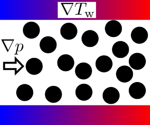
Consider a dense gas between two parallel plates at rest located respectively at $X_{1} = \pm D/2$, where $X_{i}$ are the Cartesian coordinates. The two plates are kept at the temperature $T_{w}(X_{2}) = T_{0}(1+c_{T}X_{2}/D)$ ($c_{T} = (D/T_{0})(\mathrm {d} T_{w}/\mathrm {d} X_{2})$ is a constant), and the gas is subject to some pressure gradient in the $X_{2}$ direction. We will find a solution that has a pressure gradient that is constant in the $X_{2}$ direction (but non-constant in the $X_{1}$ direction). There is no external force acting on the gas. The average density of the gas over the cross-section $X_{2} = 0$ is given by $\rho _{0}$. We will investigate the steady behaviour of the gas under the assumptions that (i) the behaviour of the gas can be described by the Enskog equation for hard-sphere molecules with a common diameter $\sigma$ and mass $m$ with the factor of pair correlation being given according to the Carnahan–Starling equation of state (Carnahan & Starling 1969); (ii) the gas molecules are diffusely reflected on the surface of the plates; (iii) the magnitudes of the applied temperature gradient $|c_{T}|$ and the pressure gradient $(D/p_{0})|\partial p/\partial X_{2}|$ are so small that the equation and boundary condition can be linearized around the state that is achieved when both gradients are absent ($p$ is the pressure, $p_{0} = \rho _{0}RT_{0}$ and $R$ is the specific gas constant).

Some comments on the appropriateness of the linearization assumption (iii) may be in order. At a glance, the assumption might look restrictive to describe the flows well. However, (a) the pressure and temperature gradients can in fact be small in small systems like micro/nano channels and porous media with small pores; (b) the assumption is actually employed also in the literature (see, e.g. any references cited in the third sentence of the fifth paragraph in § 1); (c) it is reported (see, e.g. Ohwada et al. 1989; Sharipov 2003; Ewart et al. 2007) that the results for rarefied gases obtained based on the linearized Boltzmann or model kinetic equations agree well with experimental results for a wide range of the Knudsen number. Based on these facts, the assumption is also employed here for the Enskog equation. Phenomena due to nonlinear effects, expected to be significant when the applied pressure or temperature gradient is not small, e.g. non-uniformity of temperature profile in pressure-driven flow (Zheng, Garcia & Alder 2002), are outside of the scope of the present work.

2.2. Basic equation and boundary condition

Let us denote by $\boldsymbol {X} = D\boldsymbol {x}$ the position, by $(2RT_{0})^{1/2}\boldsymbol {\zeta }$ the molecular velocity, by $\rho _{0}(2RT_{0})^{-3/2}\hat {f}$ the VDF of gas molecules, by $\sigma = D\hat {\sigma }$ the molecular diameter, by $\rho _{0}\hat {\rho }$ the density of the gas and by $T_{w}=T_{0}\hat {T}_{w}$ the temperature of the plates. Then, from assumptions (i) and (ii), the behaviour of the gas is described by the following boundary-value problem for $\hat {f}$:

(2.1a and 2.1b) $$\begin{gather} \zeta_{1}\frac{\partial{\hat{f}}}{\partial{x_{1}}} + \zeta_{2}\frac{\partial{\hat{f}}}{\partial{x_{2}}} = \frac{1}{k}\hat{Q}(\hat{f}) \quad \left(-\frac{1-\hat{\sigma}}{2} < x_{1} < \frac{1-\hat{\sigma}}{2}\right), \\ \hat{Q}(\hat{f}) = \frac{1}{2\sqrt{2{\rm \pi}}}\int \left[ \hat{Y}\left( \hat{\rho}\left( \boldsymbol{x}+\frac{1}{2}\hat{\sigma} \boldsymbol{k} \right); \eta_{0} \right)\hat{f}(\boldsymbol{x}+\hat{\sigma} \boldsymbol{k},\boldsymbol{\zeta}_{*}^{\prime})\hat{f}(\boldsymbol{x},\boldsymbol{\zeta}^{\prime}) \right. \nonumber\\ \left.- \,\hat{Y}\left( \hat{\rho}\left( \boldsymbol{x}-\frac{1}{2}\hat{\sigma} \boldsymbol{k} \right); \eta_{0} \right)\hat{f}(\boldsymbol{x}-\hat{\sigma} \boldsymbol{k},\boldsymbol{\zeta}_{*})\hat{f}(\boldsymbol{x},\boldsymbol{\zeta}) \right] \nonumber\\ \times (\hat{\boldsymbol{V}} \boldsymbol{\cdot} \boldsymbol{k})H(\hat{\boldsymbol{V}} \boldsymbol{\cdot} \boldsymbol{k}) \,\mathrm{d}\boldsymbol{k}\,\mathrm{d}\boldsymbol{\zeta}_{*}, \end{gather}$$

(2.1c) $$\begin{gather}\hat{Y}(\hat{\rho};\eta_{0}) = \frac{Y(\hat{\rho}\eta_{0})}{Y(\eta_{0})}, \quad Y(\eta) = \frac{1}{2}\frac{2-\eta}{(1-\eta)^{3}}, \quad \eta_{0} = \frac{(\rho_{0}/m){\rm \pi}\sigma^{3}}{6}, \end{gather}$$

(2.1d)$$\begin{gather}\hat{\rho} = \int \hat{f} \,\mathrm{d}\boldsymbol{\zeta}, \end{gather}$$

(2.1e)$$\begin{gather}\boldsymbol{\zeta}^{\prime} = \boldsymbol{\zeta} + (\hat{\boldsymbol{V}} \boldsymbol{\cdot} \boldsymbol{k})\boldsymbol{k}, \quad \boldsymbol{\zeta}_{*}^{\prime} = \boldsymbol{\zeta}_{*} - (\hat{\boldsymbol{V}} \boldsymbol{\cdot} \boldsymbol{k})\boldsymbol{k}, \quad \hat{\boldsymbol{V}} = \boldsymbol{\zeta}_{*} - \boldsymbol{\zeta}, \end{gather}$$

(2.1f)$$\begin{gather}k = \frac{\sqrt{\rm \pi}}{2}{Kn}, \quad {Kn} = \frac{\ell_{0}}{D}, \quad \ell_{0} = \left[ \sqrt{2}{\rm \pi}\sigma^{2}(\rho_{0}/m)Y(\eta_{0}) \right]^{-1}, \end{gather}$$

(2.1g) $$\begin{gather}\text{b.c:} \quad \hat{f} = \frac{\hat{\rho}_{w}}{(\pi\hat{T}_{w}(x_{2}))^{3/2}}\exp\left(-\frac{\zeta^2}{\hat{T}_w(x_2)}\right) \quad \left(\zeta_{1} \gtrless 0,\ x_{1} ={\mp} \frac{1-\hat{\sigma}}{2}\right), \end{gather}$$

(2.1h) $$\begin{gather}\hat{\rho}_{w} ={\mp} 2\sqrt{\frac{\rm \pi}{\hat{T}_{w}(x_{2})}}\int_{\zeta_{1}\lessgtr 0}\zeta_{1}\hat{f} \,\mathrm{d}\boldsymbol{\zeta}, \end{gather}$$

(2.1i)$$\begin{gather}\hat{T}_{w}(x_{2}) = 1+c_{T}x_{2}, \end{gather}$$

(2.1j)$$\begin{gather}\text{with} \quad\left. \frac{1}{1-\hat{\sigma}}\left( \int_{-(1-\hat{\sigma})/2}^{(1-\hat{\sigma})/2}\int \hat{f} \,\mathrm{d}\boldsymbol{\zeta}\,\mathrm{d} x_{1} \right)\right|_{x_{2}=0} = 1. \end{gather}$$

Here, $\boldsymbol {k}$ is the unit vector in the direction joining the centres of the colliding molecules, $H$ is the Heaviside function, $\eta _{0}$ and $\hat {\rho } \eta _{0}$ are the volume fractions of molecules corresponding to the average and local densities which indicate denseness of the gas and $\zeta = |\boldsymbol {\zeta }|$, respectively. The quantity $\ell _{0}$ is the mean free path of gas molecules at the equilibrium state at rest with density $\rho _{0}$ and temperature $T_{0}$. We shall use $k$ in place of the Knudsen number ${Kn}$ to indicate the degree of gas rarefaction (or smallness of the system). The operator $\hat {Q}$ is the Enskog collision integral, and it includes the parts which are quadratic in $\hat {f}$ like the Boltzmann collision integral. However, colliding molecules occupy different positions due to the finite molecular size, and the collision frequency is increased by the function $\hat {Y}$ that represents an approximate pair correlation function. Hence $\hat {Q}$ is a fivefold integral that is non-local in the position $\boldsymbol {x}$ as well as $\boldsymbol {\zeta }$ and it is more complicated than the Boltzmann collision integral which is local in $\boldsymbol {x}$. The integration in $\hat {Q}$ is carried out over the whole space of $\boldsymbol {\zeta }_{*}$ and over the whole direction of $\boldsymbol {k}$. In the integral, quantities, here the VDF $\hat {f}(\boldsymbol {x} \pm \hat {\sigma } \boldsymbol {k},\boldsymbol {\cdot })$ and the density $\hat {\rho }(\boldsymbol {x} \pm (1/2)\hat {\sigma } \boldsymbol {k})$, are read as zero if their arguments are outside of the domain $\{ \boldsymbol {z} = (z_{1},z_{2},z_{3}) | |z_{1}| \le (1-\hat {\sigma })/2 \}$. This rule is also applied to various integrals appearing later. The functional form (2.1c) of $\hat {Y}$ (or $Y$) corresponds to the Carnahan–Starling equation of state. The centre of a molecule is able to move in the domain with a width $D-\sigma$, which is narrower than the gap width $D$ by the molecular diameter $\sigma$. This fact is reflected in the collision integral (2.1b) and the condition (2.1j) as well as the equation (2.1a) and the boundary condition (2.1g).

Note that the non-dimensional numbers $k$, $\hat {\sigma }$ and $\eta _{0}$ in (2.1) are not independent but are related as (Sheng et al. 2020)

(2.2)\begin{equation} k = \frac{\sqrt{\rm \pi}}{2}\hat{\sigma}\frac{1}{6\sqrt{2}\eta_{0}Y(\eta_{0})}. \end{equation}

In the present paper, $k$ and $\hat {\sigma }$, the degree of gas rarefaction and the molecular size, are considered as the parameters of the problem. We regard the volume fraction of molecules $\eta _{0}$ as a function of $k$ and $\hat {\sigma }$ determined by (2.2). Its plot is shown in figure 1, which implies that the gas becomes more dense with the decrease of $k$ and the increase of $\hat {\sigma }$ and that it becomes less dense with the increase of $k$ and the decrease of $\hat {\sigma }$.

Figure 1. Plot of the volume fraction of molecules $\eta _{0}$ as a function of $k$ for $\hat {\sigma } = 0.001$, $0.01$, $0.05$, $0.1$ and $0.15$.

2.3. Macroscopic quantities

For later convenience, here, we introduce the macroscopic variables besides the density given by (2.1d). The flow velocity, temperature, pressure, stress tensor and heat-flow vector are given by $(2RT_{0})^{1/2}\hat {v}_{i}$, $T_{0}\hat {T}$, $p = p_{0}\hat {p}$, $p_{0}\hat {p}_{ij}$ and $p_{0}(2RT_{0})^{1/2}\hat {q}_{i}$, respectively, where $\hat {v}_{i}$, $\hat {T}$, $\hat {p}$, $\hat {p}_{ij}$ and $\hat {q}_{i}$ are defined as the following moments of the VDF $\hat {f}$:

(2.3a)$$\begin{gather} \hat{v}_{i} = \frac{1}{\hat{\rho}}\int \zeta_{i} \hat{f} \,\mathrm{d}\boldsymbol{\zeta}, \end{gather}$$

(2.3b)$$\begin{gather}\hat{T} = \frac{2}{3\hat{\rho}}\int (\zeta_{k}-\hat{v}_{k})^{2} \hat{f} \,\mathrm{d}\boldsymbol{\zeta}, \end{gather}$$

(2.3c)$$\begin{gather}\hat{p} = \hat{\rho}\hat{T} \times \frac{1+\eta+\eta^{2}-\eta^{3}}{(1-\eta)^{3}}, \quad \eta = \hat{\rho} \eta_{0}, \end{gather}$$

(2.3d) $$\begin{gather}\hat{p}_{ij} = \hat{p}_{ij}^{({k})} + \hat{p}_{ij}^{({v})}, \end{gather}$$

(2.3e) $$\begin{gather}\hat{p}_{ij}^{({k})} = 2\int (\zeta_{i}-\hat{v}_{i})(\zeta_{j}-\hat{v}_{j})\hat{f} \,\mathrm{d}\boldsymbol{\zeta},\end{gather}$$

(2.3f) $$\begin{gather} \hat{p}_{ij}^{({v})} \,{=}\, \frac{1}{2\sqrt{2{\rm \pi}}k}\iint_{0}^{\hat{\sigma}}k_{i}k_{j} \hat{Y}\left( \hat{\rho}\left( \boldsymbol{x}+\left( \frac{1}{2}\hat{\sigma}\,{-}\,\hat{\alpha} \right) \boldsymbol{k} \right){;} \eta_{0} \right) \hat{f}(\boldsymbol{x}\,{-}\,\hat{\alpha} \boldsymbol{k},\boldsymbol{\zeta}_{*}) \hat{f}(\boldsymbol{x}+(\hat{\sigma}-\hat{\alpha})\boldsymbol{k},\boldsymbol{\zeta}) \nonumber\\ \times\, (\hat{\boldsymbol{V}} \boldsymbol{\cdot} \boldsymbol{k})^{2}H(\hat{\boldsymbol{V}} \boldsymbol{\cdot} \boldsymbol{k})\,\mathrm{d}\hat{\alpha} \,\mathrm{d}\boldsymbol{k} \,\mathrm{d}\boldsymbol{\zeta} \,\mathrm{d}\boldsymbol{\zeta}_{*}, \end{gather}$$

(2.3g)$$\begin{gather}\hat{q}_{i} = \hat{q}_{i}^{({k})} + \hat{q}_{i}^{({v})}, \end{gather}$$

(2.3h) $$\begin{gather}\hat{q}_{i}^{({k})} = \int (\zeta_{i}-\hat{v}_{i})(\zeta_{k}-\hat{v}_{k})^{2}\hat{f} \,\mathrm{d}\boldsymbol{\zeta}, \end{gather}$$

(2.3i) $$\begin{gather} \hat{q}_{i}^{({v})} = \frac{1}{4\sqrt{2{\rm \pi}}k}\iint_{0}^{\hat{\sigma}} k_{i}\left[ (\zeta_{\ell}^{\prime}-\hat{v}_{\ell})^{2}-(\zeta_{\ell}-\hat{v}_{\ell})^{2} \right] \nonumber\\ \times\, \hat{Y}\left( \hat{\rho}\left( \boldsymbol{x}+\left( \frac{1}{2}\hat{\sigma}-\hat{\alpha} \right) \boldsymbol{k} \right); \eta_{0} \right) \hat{f}(\boldsymbol{x}-\hat{\alpha} \boldsymbol{k},\boldsymbol{\zeta}_{*})\hat{f}(\boldsymbol{x}+(\hat{\sigma}-\hat{\alpha})\boldsymbol{k},\boldsymbol{\zeta}) \nonumber\\ \times \,(\hat{\boldsymbol{V}} \boldsymbol{\cdot} \boldsymbol{k})H(\hat{\boldsymbol{V}} \boldsymbol{\cdot} \boldsymbol{k})\,\mathrm{d}\hat{\alpha} \,\mathrm{d}\boldsymbol{k} \,\mathrm{d}\boldsymbol{\zeta} \,\mathrm{d}\boldsymbol{\zeta}_{*}. \end{gather}$$

Equation (2.3c) is the Carnahan–Starling equation of state. The stress tensor $\hat {p}_{ij}$ and the heat-flow vector $\hat {q}_{i}$ are given by a sum of two parts, respectively. The first part, $\hat {p}_{ij}^{({k})}$ and $\hat {q}_{i}^{({k})}$, is called the kinetic part and has a familiar form. The second part, $\hat {p}_{ij}^{({v})}$ and $\hat {q}_{i}^{({v})}$, is called the potential part (Cercignani & Lampis 1988), and it represents the contribution of instantaneous transfers of momentum and energy in binary collisions.

2.4. Linearization

Recalling that we consider the situation where the applied temperature and pressure gradients are small (see assumption (iii) in § 2.1), within the linearized regime, we can seek the solution $\hat {f}$ of problem (2.1) as a sum of reference state and perturbation, as follows:

(2.4a)$$\begin{gather} \hat{f} = \hat{M}(x_{1},\boldsymbol{\zeta}) + \varPhi(x_{1},x_{2},\boldsymbol{\zeta}) + O(\varPhi^{2}) \quad (|\varPhi| \ll \hat{M}), \end{gather}$$

(2.4b)$$\begin{gather}\hat{M} = \hat{\rho}_{M}(x_{1})E(\zeta), \quad E(\zeta) = {\rm \pi}^{-3/2}e^{-\zeta^{2}}, \end{gather}$$

(2.4c) $$\begin{gather} \varPhi = c_{T}\left\{ x_{2}E(\zeta)\left[ \hat{\omega}_{T}(x_{1})+\left(\zeta^{2}-\frac{3}{2}\right)\hat{\rho}_{M}(x_{1}) \right] + \varPsi_{T}(x_{1},\boldsymbol{\zeta}) \right\}\nonumber\\ +\, c_{P}\left[ x_{2}E(\zeta)\hat{\omega}_{P}(x_{1}) + \varPsi_{P}(x_{1},\boldsymbol{\zeta}) \right]. \end{gather}$$

Here, some notes may be in order:

1. (i) The function $\hat {M}$ is the reference state of the gas that is achieved when both the temperature and pressure gradients are absent, i.e. when there is no driving factor in the system. While for an ideal gas (the case of the Boltzmann equation) this state is a uniform equilibrium state at rest, for a dense gas it is an equilibrium state at rest with a density distribution $\hat {\rho }_{M}(x_{1})$ varying in the direction normal to the plates (Frezzotti (1997); see also figure 2(a) shown later). The non-uniformity of the reference density is attributed to the fact that some of intermolecular collisions which detach the molecules from the plates are forbidden near the boundary due to their finite size and accordingly they are pushed to the plates.

2. (ii) The function $\varPhi$ is a perturbation around the reference state $\hat {M}$. In its expression, the subscripts $T$ and $P$ are attached to discriminate the quantities related to the thermal transpiration and Poiseuille flows, respectively. The $O(\varPhi ^{2})$ term in (2.4a) is the negligible error in the linearized regime. As will be seen later in § 4, when the molecular size $\hat {\sigma }$ is finite, the pressure gradient $\partial _{x_{2}}\hat {p}$ and the stress gradient $\partial _{x_{2}}\hat {p}_{22}$ are not identical, and moreover they are non-uniform in $x_{1}$. Here, the latter is regarded as the driving force for the Poiseuille flow since it is the stress rather than the pressure that has the role of the mechanical surface force. Thus, we require that its average in the $x_{1}$ direction be normalized and zero, in accordance with the nature of the Poiseuille and thermal transpiration flows, respectively. To be more precise, with $\hat {p}_{22}$ being evaluated with $\hat {f} = \hat {M} + \varPhi$, we require that $(1-\hat {\sigma })^{-1}\int _{-(1-\hat {\sigma })/2}^{(1-\hat {\sigma })/2}\partial _{x_{2}}\hat {p}_{22}|_{c_{T}=0}\,\mathrm {d} x_{1} = c_{P}$ and $(1-\hat {\sigma })^{-1}\int _{-(1-\hat {\sigma })/2}^{(1-\hat {\sigma })/2}\partial _{x_{2}}\hat {p}_{22}|_{c_{P}=0}\,\mathrm {d} x_{1} = 0$ for respective flows, where the constant $c_{P}$ represents the magnitude of the averaged stress gradient in the Poiseuille flow ($|c_{P}| \ll 1$ by assumption (iii)). Since $\partial _{x_{2}}\hat {p}_{22} = \partial _{x_{2}}\hat {p} = \mathrm {const.}$ for the Boltzmann equation, $c_{P}$ also corresponds to the magnitude of the pressure gradient $(D/p_{0})|\,\mathrm {d} p/\mathrm {d} X_{2}|$ in this case. The parts $c_{P}x_{2}E(\zeta )\hat {\omega }_{P}(x_{1})$ and $c_{T}x_{2}E(\zeta )[\hat {\omega }_{T}(x_{1})+(\zeta ^{2}-\frac {3}{2})\hat {\rho }_{M}(x_{1})]$ are the perturbed Maxwellians representing the pressure (or stress) and temperature gradients, respectively. Recall that the magnitude of the latter is represented by the coefficient $c_{T}[= (D/T_{0})(\mathrm {d} T_{w}/\mathrm {d} X_{2})]$. The functions $\varPsi _{T}$ and $\varPsi _{P}$, which are considered to be odd in $\zeta _{2}$, represent the respective flows.

3. (iii) The expression (2.4) might look like an arbitrary assumption at a glance, however, it turns out to be an appropriate form of the solution. It is an extension of the similarity solution for a rarefied gas (see also, e.g. (2.8) in Takata & Funagane (2011) or (1) in Ohwada et al. 1989) to the case of the dense gas, where the non-uniformity of densities in $x_{1}$ is taken into account here due to the finite molecular size both for the reference part $\hat {\rho }_{M}$ and the perturbed parts $\hat {\omega }_{T,P}$ (the case of Boltzmann equation corresponds to the case $\hat {\rho }_{M}(x_{1}) \equiv 1$, $\hat {\omega }_{T}(x_{1}) \equiv -1$ and $\hat {\omega }_{P}(x_{1}) \equiv 1$). To confirm the consistency of (2.4), actually we can proceed in the following way, which is detailed in Appendix A. First, substitute $\hat {f} = \hat {M} = \hat {\rho }_{M}E$ into the equation (2.1a) and the condition for average density (2.1j). Then, we reach the system which determines the reference density $\hat {\rho }_{M}$ (and $\hat {M}$ accordingly) with no inconsistency. Second, introduce the perturbation $\varPhi$ and substitute $\hat {f} = \hat {M} + \varPhi$ (see also (2.4a)) into the equation (2.1a), the boundary condition (2.1g) and the condition for average density (2.1j), and neglect the second- and higher-order terms of perturbation $\varPhi$ according to assumption (iii). Then, we are left with the linearized system for the perturbation $\varPhi$, without any inconsistency. Third, substitute the expression (2.4c) into the system for $\varPhi$ and closely examine the resulting expressions, in particular those of the collision integral. Then, we find that the form (2.4c) introduces no inconsistency, and the systems for the perturbed densities $\hat {\omega }_{T, P}$ and the VDFs $\varPsi _{T, P}$ are accordingly obtained.

Figure 2. Profiles of quantities related to the density and the gradients of the pressure and the $(2,2)$ component of stress; (a) $\hat {\rho }_{M}$, (b) $\hat {\omega }_{T}$ and $\hat {\omega }_{P}$, (c) $G_{T}$, (d) $G_{{22},T}^{({k})} + G_{22,T}^{({v})}$, (e) $G_{P}$ and ( f) $G_{{22},P}^{({k})} + G_{22,P}^{({v})}$.

2.4.1. Problems of $\hat {\rho }_{M}$, $\hat {\omega }_{T, P}$ and $\varPsi _{T, P}$

In (2.4), $\hat {\rho }_{M}$, $\hat {\omega }_{T, P}$ and $\varPsi _{T, P}$ are the functions to be determined. Following the above steps explained in the item (iii) or Appendix A, we find that the densities $\hat {\rho }_{M}$, $\hat {\omega }_{T}$ and $\hat {\omega }_{P}$ satisfy the following integro-differential equations, while the VDFs $\varPsi _{T}$ and $\varPsi _{P}$ are the solutions of the following boundary-value problems of the linearized Enskog equation:

(2.5a)$$\begin{gather} \frac{\mathrm{d} \hat{\rho}_{M}(x_{1})}{\mathrm{d} x_{1}} = J_{1}[\hat{\rho}_{M}](x_{1}) \quad \left(-\frac{1-\hat{\sigma}}{2} < x_{1} < \frac{1-\hat{\sigma}}{2}\right), \end{gather}$$

(2.5b)$$\begin{gather}\text{with} \quad \frac{1}{1-\hat{\sigma}}\int_{-(1-\hat{\sigma})/2}^{(1-\hat{\sigma})/2}\hat{\rho}_{M}(x_{1})\,\mathrm{d} x_{1} = 1, \end{gather}$$

(2.6a)$$\begin{gather} \frac{\mathrm{d} \hat{\omega}_{\beta}(x_{1})}{\mathrm{d} x_{1}} = K_{1}[\hat{\omega}_{\beta},\hat{\rho}_{M}](x_{1}) \quad \left(-\frac{1-\hat{\sigma}}{2} < x_{1} < \frac{1-\hat{\sigma}}{2}\right), \end{gather}$$

(2.6b)$$\begin{gather}\text{with} \quad K_{2}[\hat{\omega}_{T}, \hat{\rho}_{M}] = J_{2}[\hat{\rho}_{M}] - 1, \end{gather}$$

(2.6c)$$\begin{gather}K_{2}[\hat{\omega}_{P}, \hat{\rho}_{M}] = 1, \end{gather}$$

(2.7a)$$\begin{gather} \zeta_{1}\frac{\partial{\varPsi_{\beta}}}{\partial{x_{1}}} = \frac{1}{k}L(\varPsi_{\beta}) + I_{\beta} \quad \left(-\frac{1-\hat{\sigma}}{2} < x_{1} < \frac{1-\hat{\sigma}}{2}\right), \end{gather}$$

(2.7b)$$\begin{gather}\text{b.c.} \quad \varPsi_{\beta} = 0 \quad \left(\zeta_{1} \gtrless 0,\ x_{1} ={\mp} \frac{1-\hat{\sigma}}{2}\right). \end{gather}$$

Here, $\beta = T, P$ in (2.6a) and (2.7). The operators $J_{1}$, $J_{2}$ and $J_{3}$ appearing in (2.5a), (2.6b) and the definition (2.11a) of the source term $I_{T}$ shown later are integrals of $\hat {\rho }_{M}$ given by (B1) in Appendix B. The operators $K_{1}$, $K_{2}$ and $K_{3}$ appearing in (2.6) and the definition (2.11) of $I_{\beta }$ are integrals that are linear with respect to $\hat {\omega }_{\beta }$ given by (B3) in Appendix B. The integrals $J_{1}$ and $K_{1}$ represent the contribution coming from the collision integral $\hat {Q}$ to the densities $\hat {\rho }_{M}$ and $\hat {\omega }_{\beta }$. Equations (2.6c) and (2.6b) are the reduced form of the aforementioned conditions on the stress gradient $\partial _{x_{2}}\hat {p}_{22}$ explained in the item (ii) of § 2.4 (see also the last paragraph in Appendix A.3). By these conditions (2.6c) and (2.6b), $\hat {\omega }_{P}$ and $\hat {\omega }_{T}$, which satisfy the same linear equation (2.6a) and are thus equal up to a multiplicative constant, are distinguished from each other. The quantity $L$ appearing in (2.7a) is the following Enskog collision operator linearized around the reference local equilibrium state $\hat {M}(x_{1},\boldsymbol {\zeta })$:

(2.8a)$$\begin{gather} L(\psi)(\boldsymbol{x},\boldsymbol{\zeta}) = C(\psi)(\boldsymbol{x},\boldsymbol{\zeta}) - \nu(x_{1},\boldsymbol{\zeta})\psi(\boldsymbol{x},\boldsymbol{\zeta}), \end{gather}$$

(2.8b) $$\begin{align} C(\psi)(\boldsymbol{x},\boldsymbol{\zeta})&= \frac{1}{2\sqrt{2{\rm \pi}}}\int \left\{\hat{Y}\left( {\hat{\rho}_{M}\left( {x_{1}+\frac{{1}}{{2}}\hat{\sigma} k_{1}} \right); \eta_{0}} \right) \right. \nonumber\\ &\quad\times \left[\hat{M}(x_{1}+\hat{\sigma} k_{1},\boldsymbol{\zeta}_{*}^{\prime})\psi(\boldsymbol{x},\boldsymbol{\zeta}^{\prime}) +\psi(\boldsymbol{x}+\hat{\sigma} \boldsymbol{k},\boldsymbol{\zeta}_{*}^{\prime})\hat{M}(x_{1},\boldsymbol{\zeta}^{\prime})\right] \nonumber\\ &\quad-\hat{Y}\left( {\hat{\rho}_{M}\left( {x_{1}-\frac{{1}}{{2}}\hat{\sigma} k_{1}} \right); \eta_{0}} \right) \psi(\boldsymbol{x}-\hat{\sigma} \boldsymbol{k},\boldsymbol{\zeta}_{*})\hat{M}(x_{1},\boldsymbol{\zeta}) \nonumber\\ &\quad+\hat{Y}_{1}\left( {\hat{\rho}_{M}\left( {x_{1}+\frac{{\hat{\sigma}}}{{2}} k_{1}} \right); \eta_{0}} \right) \left\langle \psi \right\rangle\left(\boldsymbol{x}+\frac{\hat{\sigma}}{2} \boldsymbol{k}\right)\hat{M}(x_{1}+\hat{\sigma} k_{1},\boldsymbol{\zeta}_{*}^{\prime})\hat{M}(x_{1},\boldsymbol{\zeta}^{\prime}) \nonumber\\ &\quad\left.\left.-\,\hat{Y}_{1}\left( {\hat{\rho}_{M}\left( {x_{1}-\frac{{\hat{\sigma}}}{{2}} k_{1}} \right); \eta_{0}} \right) \left\langle \psi \right\rangle\left(\boldsymbol{x}-\frac{\hat{\sigma}}{2} \boldsymbol{k}\right)\hat{M}(x_{1}-\hat{\sigma} k_{1},\boldsymbol{\zeta}_{*})\hat{M}(x_{1},\boldsymbol{\zeta})\right] \right\} \nonumber\\ &\quad\times (\hat{\boldsymbol{V}} \boldsymbol{\cdot} \boldsymbol{k})H(\hat{\boldsymbol{V}} \boldsymbol{\cdot} \boldsymbol{k}) \,\mathrm{d}\boldsymbol{k}\,\mathrm{d}\boldsymbol{\zeta}_{*}, \end{align}$$

(2.8c) $$\begin{gather} \nu(x_{1},\boldsymbol{\zeta})= \frac{1}{2\sqrt{2{\rm \pi}}}\int \hat{Y}\left( {\hat{\rho}_{M}\left( {x_{1}-\frac{{1}}{{2}}\hat{\sigma} k_{1}} \right); \eta_{0}} \right)\nonumber\\ \times\, \hat{M}(x_{1}-\hat{\sigma} k_{1},\boldsymbol{\zeta}_{*}) (\hat{\boldsymbol{V}} \boldsymbol{\cdot} \boldsymbol{k})H(\hat{\boldsymbol{V}} \boldsymbol{\cdot} \boldsymbol{k}) \,\mathrm{d}\boldsymbol{k}\,\mathrm{d}\boldsymbol{\zeta}_{*}, \end{gather}$$

where

(2.9a)$$\begin{gather} \hat{Y}_{1}\left( r; \eta_{0} \right) = \frac{1}{Y(\eta_{0})}\frac{\eta_{0}(5-2r\eta_{0})}{2(1-r\eta_{0})^{4}}, \end{gather}$$

(2.9b)$$\begin{gather}\left\langle \psi \right\rangle(\boldsymbol{x}) = \int \psi(\boldsymbol{x},\boldsymbol{\zeta}) \,\mathrm{d}\boldsymbol{\zeta}. \end{gather}$$

In the decomposition (2.8a) of $L$, $C$ is the integral operator with some smoothing property in the molecular velocity $\boldsymbol {\zeta }$ and $\nu$ is the collision frequency for the reference equilibrium state $\hat {M}(x_{1},\boldsymbol {\zeta })$. The function $\hat {Y}_{1}$ given in (2.9a) is just a perturbed part of $\hat {Y}$ such that

(2.10)\begin{equation} \hat{Y}(\hat{\rho}_{M}+c\left\langle \psi \right\rangle;\eta_{0}) = \hat{Y}(\hat{\rho}_{M};\eta_{0}) + c\left\langle \psi \right\rangle\hat{Y}_{1}(\hat{\rho}_{M};\eta_{0}) + O(c^{2}) \ (|c| \ll 1). \end{equation}

The source term $I_{\beta }$ in (2.7a) is given in terms of the densities $\hat {\rho }_{M}$ and $\hat {\omega }_{T,P}$ as

(2.11a) $$\begin{gather} I_{T}(x_{1},\boldsymbol{\zeta}) =-\zeta_{2}E(\zeta)\left[ \hat{\rho}_{M}(x_{1})\left(\zeta^{2}-\frac{3}{2}\right) + \hat{\omega}_{T}(x_{1}) \right]\nonumber\\ -\,\frac{\hat{\sigma} E(\zeta)}{k2\sqrt{2{\rm \pi}}}\left\{\zeta_{2}K_{3}[\hat{\omega}_{T}, \hat{\rho}_{M}](x_{1}) +J_{3}[\hat{\rho}_{M}](x_{1},\boldsymbol{\zeta})\right\}, \end{gather}$$

(2.11b)$$\begin{gather}I_{P}(x_{1},\boldsymbol{\zeta}) =-\zeta_{2}E(\zeta) \hat{\omega}_{P}(x_{1}) - \frac{\hat{\sigma}}{k2\sqrt{2{\rm \pi}}}\zeta_{2} E(\zeta) K_{3}[\hat{\omega}_{P}, \hat{\rho}_{M}](x_{1}). \end{gather}$$

Thanks to the symmetry of the present problem with respect to the middle of the gap $x_{1} = 0$, we can seek the VDF $\varPsi _{\beta }$ with the following property:

(2.12)\begin{equation} \varPsi_{\beta}(x_{1},\zeta_{1},\zeta_{2},\zeta_{3}) = \varPsi_{\beta}(-x_{1},-\zeta_{1},\zeta_{2},\zeta_{3}) \quad \left(0 < x_{1} < \frac{1-\hat{\sigma}}{2}; \beta = T, P\right). \end{equation}

Thus, hereafter, we impose the following condition:

(2.13)\begin{equation} \varPsi_{\beta}(0,\zeta_{1},\zeta_{2},\zeta_{3}) = \varPsi_{\beta}(0,-\zeta_{1},\zeta_{2},\zeta_{3}) \end{equation}

on $\varPsi _{\beta }$, which is obtained by substituting $x_{1} = 0$ into (2.12), and we consider the problem of $\varPsi _{\beta }$ on $-(1-\hat {\sigma })/2 < x_{1} < 0$.

2.4.2. Expressions of macroscopic quantities

Substituting the solution (2.4) into (2.1d), (2.3a)–(2.3c), (2.3e), (2.3f), (2.3h) and (2.3i), within negligible error $O(c_{P}^{2},c_{T}^{2})$ in the linearized regime, we have the following expressions for the macroscopic quantities $\hat {\rho }$, $\hat {v}_{i}$, $\hat {T}$, $\hat {p}$, $\hat {p}_{ij}^{({k})}$, $\hat {p}_{ij}^{({v})}$, $\hat {q}_{i}^{({k})}$ and $\hat {q}_{i}^{({v})}$:

(2.14a)$$\begin{gather} \hat{\rho} = \hat{\rho}_{M}(x_{1}) + c_{T}x_{2}\hat{\omega}_{T}(x_{1}) + c_{P}x_{2}\hat{\omega}_{P}(x_{1}) + O(c_{P}^{2},c_{T}^{2}), \end{gather}$$

(2.14b)$$\begin{gather}\hat{v}_{2} = c_{T}u[\varPsi_{T}](x_{1}) + c_{P}u[\varPsi_{P}](x_{1}) + O(c_{P}^{2},c_{T}^{2}), \end{gather}$$

(2.14c)$$\begin{gather}\hat{v}_{1} = O(c_{P}^{2},c_{T}^{2}), \quad \hat{v}_{3} = O(c_{P}^{2},c_{T}^{2}), \end{gather}$$

(2.14d)$$\begin{gather}\hat{T} = 1 + c_{T}x_{2} + O(c_{P}^{2},c_{T}^{2}), \end{gather}$$

(2.14e)$$\begin{gather}\hat{p} = \hat{\rho}_{M}(x_{1})S_{1}(\hat{\rho}_{M}(x_{1})\eta_{0}) + c_{T}x_{2}G_{T}(x_{1}) + c_{P}x_{2}G_{P}(x_{1}) + O(c_{P}^{2},c_{T}^{2}), \end{gather}$$

(2.14f)$$\begin{gather}\hat{p}_{22}^{({k})} = \hat{\rho}_{M}(x_{1}) + c_{T}x_{2}G_{{22},T}^{({k})}(x_{1}) + c_{P}x_{2}G_{{22},P}^{({k})}(x_{1}) + O(c_{P}^{2},c_{T}^{2}), \end{gather}$$

(2.14g) $$\begin{gather}\hat{p}_{12}^{({k})} = c_{T}P_{12}^{({k})}[\varPsi_{T}](x_{1}) + c_{P}P_{12}^{({k})}[\varPsi_{P}](x_{1}) + O(c_{P}^{2},c_{T}^{2}), \end{gather}$$

(2.14h) $$\begin{gather} \hat{p}_{11}^{({k})} = \hat{p}_{22}^{({k})}+O(c_{P}^{2},c_{T}^{2}), \quad \hat{p}_{33}^{({k})} = \hat{p}_{22}^{({k})}+ O(c_{P}^{2},c_{T}^{2}), \nonumber \\ \hat{p}_{13}^{({k})} = O(c_{P}^{2},c_{T}^{2}), \quad \hat{p}_{23}^{({k})} = O(c_{P}^{2},c_{T}^{2}), \end{gather}$$

(2.14i) $$\begin{gather}\hat{p}_{11}^{({v})} = P_{11,M}^{({v})}(x_{1}) + c_{T}x_{2}G_{11,T}^{({v})}(x_{1}) + c_{P}x_{2}G_{11,P}^{({v})}(x_{1}) + O(c_{P}^{2},c_{T}^{2}), \end{gather}$$

(2.14j) $$\begin{gather}\hat{p}_{22}^{({v})} = P_{22,M}^{({v})}(x_{1}) + c_{T}x_{2}G_{22,T}^{({v})}(x_{1}) + c_{P}x_{2}G_{22,P}^{({v})}(x_{1}) + O(c_{P}^{2},c_{T}^{2}), \end{gather}$$

(2.14k)$$\begin{gather}\hat{p}_{12}^{({v})} = c_{T}P_{12,T}^{({v})}(x_{1}) + c_{P}P_{12,P}^{({v})}(x_{1}) + O(c_{P}^{2},c_{T}^{2}), \end{gather}$$

(2.14l)$$\begin{gather}\hat{p}_{33}^{({v})} = \hat{p}_{22}^{({v})} + O(c_{P}^{2},c_{T}^{2}), \quad \hat{p}_{13}^{({v})} = O(c_{P}^{2},c_{T}^{2}), \quad \hat{p}_{23}^{({v})} = O(c_{P}^{2},c_{T}^{2}), \end{gather}$$

(2.14m)$$\begin{gather}\hat{q}_{2}^{({k})} = c_{T}Q^{({k})}[\varPsi_{T}](x_{1}) + c_{P}Q^{({k})}[\varPsi_{P}](x_{1}) + O(c_{P}^{2},c_{T}^{2}), \end{gather}$$

(2.14n)$$\begin{gather}\hat{q}_{2}^{({v})} = c_{T}Q_{T}^{({v})}(x_{1}) + c_{P}Q_{P}^{({v})}(x_{1}) + O(c_{P}^{2},c_{T}^{2}), \end{gather}$$

(2.14o)$$\begin{gather}\hat{q}_{1}^{({k})} = O(c_{P}^{2},c_{T}^{2}), \quad \hat{q}_{3}^{({k})} = O(c_{P}^{2},c_{T}^{2}), \quad \hat{q}_{1}^{({v})} = O(c_{P}^{2},c_{T}^{2}), \quad \hat{q}_{3}^{({v})} = O(c_{P}^{2},c_{T}^{2}). \end{gather}$$

Here,

(2.15a)$$\begin{gather} u[\varPsi_{\beta}] = \frac{1}{\hat{\rho}_{M}}\int \zeta_{2}\varPsi_{\beta} \,\mathrm{d}\boldsymbol{\zeta}, \end{gather}$$

(2.15b)$$\begin{gather}G_{T} = \hat{\rho}_{M}(x_{1})S_{1}(\hat{\rho}_{M}(x_{1})\eta_{0}) + \hat{\omega}_{T}(x_{1})[S_{1}(\hat{\rho}_{M}(x_{1})\eta_{0})+S_{2}(\hat{\rho}_{M}(x_{1})\eta_{0})], \end{gather}$$

(2.15c)$$\begin{gather}G_{P} = \hat{\omega}_{P}(x_{1})[S_{1}(\hat{\rho}_{M}(x_{1})\eta_{0})+S_{2}(\hat{\rho}_{M}(x_{1})\eta_{0})], \end{gather}$$

(2.15d)$$\begin{gather}S_{1}(r) = \frac{1+r+r^{2}-r^{3}}{(1-r)^{3}}, \quad S_{2}(r) = \frac{2r(2+2r-r^{2})}{(1-r)^{4}}, \end{gather}$$

(2.15e)$$\begin{gather}G_{{22},T}^{({k})} = \hat{\rho}_{M}(x_{1}) + \hat{\omega}_{T}(x_{1}), \quad G_{{22},P}^{({k})} = \hat{\omega}_{P}(x_{1}), \end{gather}$$

(2.15f)$$\begin{gather}P_{12}^{({k})}[\varPsi_{\beta}] = 2\int \zeta_{1}\zeta_{2}\varPsi_{\beta} \,\mathrm{d}\boldsymbol{\zeta}, \end{gather}$$

(2.15g)$$\begin{gather}P_{12,\beta}^{({v})}(x_{1}) = P_{12,\omega_{\beta}}^{({v})}(x_{1}) + P_{12}^{({v})}[\varPsi_{\beta}](x_{1}), \end{gather}$$

(2.15h)$$\begin{gather}Q^{({k})}[\varPsi_{\beta}] = \int \zeta_{2}\left( \zeta^{2}-\frac{5}{2} \right)\varPsi_{\beta} \,\mathrm{d}\boldsymbol{\zeta}, \end{gather}$$

(2.15i)$$\begin{gather}Q_{T}^{({v})} = Q^{({v})}[\varPsi_{T}](x_{1}) - \left\{ u[\varPsi_{T}](x_{1}) + \frac{\hat{\sigma}}{\sqrt{2{\rm \pi}}} \right\}P_{22,M}^{({v})}(x_{1}), \end{gather}$$

(2.15j)$$\begin{gather}Q_{P}^{({v})} = Q^{({v})}[\varPsi_{P}](x_{1}) - u[\varPsi_{P}](x_{1})P_{22,M}^{({v})}(x_{1}). \end{gather}$$

The expressions of the stress contributions $P_{11,M}^{({v})}$, $P_{22,M}^{({v})}$, $P_{12,\omega _{T}}^{({v})}$ and $P_{12,\omega _{P}}^{({v})}$ and the gradients $G_{11,T}^{({v})}$, $G_{11,P}^{({v})}$, $G_{22,T}^{({v})}$ and $G_{22,P}^{({v})}$, which are all defined as the integrals of the densities $\hat {\rho }_{M}$, $\hat {\omega }_{T}$ and $\hat {\omega }_{P}$, and those of $P_{12}^{({v})}[\varPsi _{\beta }]$ and $Q^{({v})}[\varPsi _{\beta }]$, are given in Appendix C. Note that $c_{T}G_{T}$, $c_{T}(G_{{22},T}^{({k})}+G_{{22},T}^{({v})})$ and $c_{T}(Q^{({k})}[\varPsi _{T}]+Q_{T}^{({v})})$ (or $c_{P}G_{P}$, $c_{P}(G_{{22},P}^{({k})}+G_{{22},P}^{({v})})$ and $c_{P}(Q^{({k})}[\varPsi _{P}]+Q_{P}^{({v})})$) are the gradient of pressure $\partial _{x_{2}}\hat {p}$, that of the $(2,2)$ component of stress $\partial _{x_{2}}\hat {p}_{22}$ and the heat flow $\hat {q}_{2}$ for the thermal transpiration (or Poiseuille) flow, respectively, within the linearized regime (see (2.14e), (2.3d), (2.14f), (2.14j), (2.3g), (2.14m) and (2.14n)).

It is better to mention again the expression (2.14) is obtained within the linearized regime. At a glance, it might look strange that the temperature $\hat {T}$ is uniform for the Poiseuille flow and that the diagonal kinetic-part stress components are equal to each other (see (2.14d) with $c_{T} = 0$ and (2.14h)). However, they are justified in the linearized regime, and deviations from them are attributed to nonlinear effects of $O(c_{P}^{2},c_{T}^{2})$, which are neglected here due to the smallness (see also the last sentence in § 2.1). The coefficients $c_{P,T}$ need to be sufficiently small compared with 1, and, in addition, compared with the degree of gas rarefaction $k$ when we consider the flow with small $k$. (Some of the quantities of interest in the present paper are of $O(k)$ rather than $O(1)$.) Although there is no definite threshold, e.g. when $c_{P,T} \lesssim 0.001$ or $c_{P,T} \lesssim 0.0001$, the nonlinear effects would likely not be significant for the cases presented in § 4, where $k$ is in the range $[0.05, 10]$.

Also, as in other works based on the linearization assumption, flows between two infinitely wide parallel plates are considered in the present work. Thus, when flow in a finite-length channel with moderate pressure and temperature differences is considered, its length (and the lateral width when a rectangular channel is considered as in experiments) needs to be sufficiently long compared with both its gap width $D$ and the mean free path so that the results for infinitely wide plates give a good description of the flow (Sharipov 1999). Note that, for the case of a rarefied gas, there is an experiment of pressure-driven flow (Ewart et al. 2007) taking this condition carefully into consideration (the channel length and lateral width are respectively approximately 1000 and 52 times the gap width). There, it is reported that the experimental results agree well with numerical results for infinitely wide plates (Loyalka 1975) based on a model kinetic equation for a wide range of the Knudsen number approximately up to $10$.

2.4.3. Net mass flow and conservation law

Denoting by $\rho _{0}(2RT_{0})^{1/2}D\mathcal {M}$ the net mass flow through the gap per unit time and unit length in $X_{3}$, $\mathcal {M}$ is given as

(2.16)\begin{equation} \mathcal{M} = c_{T}\mathcal{M}_{T} + c_{P}\mathcal{M}_{P} + O(c_{P}^{2},c_{T}^{2}), \end{equation}

where

(2.17)\begin{equation} \mathcal{M}_{\beta} = \int_{-(1-\hat{\sigma})/2}^{(1-\hat{\sigma})/2}\hat{\rho}_{M}(s)u[\varPsi_{\beta}](s)\,\mathrm{d} s. \end{equation}

Multiplying (2.1a) by $\zeta _{2}$ and integrating the result over the whole space of $\boldsymbol {\zeta }$, we have the following conservation equation for the momentum in the $x_{2}$ direction within negligible error in the linearized regime:

(2.18)\begin{equation} \frac{\partial{\hat{p}_{12}}}{\partial{x_{1}}} + \frac{\partial{\hat{p}_{22}}}{\partial{x_{2}}} = O(c_{P}^{2},c_{T}^{2}). \end{equation}

Substituting the expression of $\hat {p}_{12}$ and $\hat {p}_{22}$ (see (2.3d), (2.14f), (2.14g), (2.14j) and (2.14k)) into (2.18) and integrating the result over [$-(1-\hat {\sigma })/2$, $x_{1}$] with respect to $x_{1}$, we obtain

(2.19)\begin{equation} c_{T}S_{T}(x_{1}) + c_{P}S_{P}(x_{1})= O(c_{P}^{2},c_{T}^{2}), \end{equation}

where

(2.20) $$\begin{gather} S_{\beta}(x_{1}) = P_{12}^{({k})}[\varPsi_{\beta}](x_{1}) + P_{12,\beta}^{({v})}(x_{1}) - P_{12}^{({k})}[\varPsi_{\beta}]\left(-\frac{1-\hat{\sigma}}{2}\right) \nonumber\\ + \int_{-(1-\hat{\sigma})/2}^{x_{1}}\left[ G_{{22},\beta}^{({k})}(s) + G_{22,\beta}^{({v})}(s) \right]\,\mathrm{d} s. \end{gather}$$

In obtaining (2.20), we have used the fact that the potential part of the stress $P_{12,\beta }^{({v})}$ vanishes on the boundary $x_{1} = -(1-\hat {\sigma })/2$. The relation (2.19) will be used for the accuracy test of our computation.

3. Numerical method

The densities $\hat {\rho }_{M}$, $\hat {\omega }_{T}$ and $\hat {\omega }_{P}$, which are defined by (2.5) and (2.6), can be obtained numerically by the method in Frezzotti (1997). Thus, the problem is reduced to (2.7) with (2.13) for the VDFs $\varPsi _{T}$ and $\varPsi _{P}$.

Let us explain the numerical solution method for the problems of $\varPsi _{T}$ and $\varPsi _{P}$. We solve them by using iteration based on the integral formulation (Takata & Funagane 2011; Hattori & Takata 2015) of the Enskog equation combined with the fast Fourier spectral method (Filbet et al. 2006) for the computation of the collision integral. Taking into account (2.8a) and (2.13) and formally integrating the equation (2.7a) with respect to $x_{1}$, we have

(3.1a) \begin{align} \varPsi_{\beta}(x_{1},\boldsymbol{\zeta}) &= \int_{-(1-\hat{\sigma})/2}^{x_{1}}\left[ \frac{1}{k\zeta_{1}}C(\varPsi_{\beta})(s,\boldsymbol{\zeta}) + \frac{1}{\zeta_{1}}I_{\beta}(s,\boldsymbol{\zeta}) \right]\exp\left( -\frac{1}{k\zeta_{1}}\int_{s}^{x_{1}}\nu(\,p,\boldsymbol{\zeta})\,\mathrm{d} p \right)\,\mathrm{d} s,\nonumber\\ &\quad \left(-\frac{1-\hat{\sigma}}{2} < x_{1} < 0,\ \zeta_{1} > 0\right), \end{align}

(3.1b) \begin{align} \varPsi_{\beta}(x_{1},\boldsymbol{\zeta}) &= \varPsi_{\beta}(0,\boldsymbol{\zeta}^-)\exp\left( -\frac{1}{k\zeta_{1}}\int_{0}^{x_{1}}\nu(\,p,\boldsymbol{\zeta})\,\mathrm{d} p \right) \nonumber\\ &\quad+\int_{0}^{x_{1}}\left[ \frac{1}{k\zeta_{1}}C(\varPsi_{\beta})(s,\boldsymbol{\zeta}) + \frac{1}{\zeta_{1}}I_{\beta}(s,\boldsymbol{\zeta}) \right]\exp\left( -\frac{1}{k\zeta_{1}}\int_{s}^{x_{1}}\nu(\,p,\boldsymbol{\zeta})\,\mathrm{d} p \right)\,\mathrm{d} s,\nonumber\\ &\quad \left(-\frac{1-\hat{\sigma}}{2} < x_{1} < 0,\ \zeta_{1} < 0\right), \end{align}

where $\boldsymbol {\zeta }^- = (-\zeta _{1}, \zeta _{2}, \zeta _{3})$ and $\beta = T, P$. Since $C$ is an integral operator, $C(\varPsi _{\beta })$ is mild in $\boldsymbol {\zeta }$ even if its argument function $\varPsi _{\beta }$ is not. Thus, the factor of steep variation of $\varPsi _{\beta }$ in $\boldsymbol {\zeta }$ (or $\zeta _{1}$) is explicit in this formulation, which will be advantageous in accurately capturing the structure of the solution. The solution $\varPsi _{\beta }$ is constructed by iteration based on (3.1) from its initial guess. The data of $C(\varPsi _{\beta })$ are computed by the fast Fourier spectral method from the given data of $\varPsi _{\beta }$. The fast Fourier spectral method for the nonlinear Enskog collision integral is explained in Wu et al. (2015). Following the reference, we can prepare the method for the linearized Enskog collision operator $C$ in the present work. The spatial integration with respect to $p$ and that with respect to $s$ in (3.1) are performed analytically after $\nu$ and $(C(\varPsi _{\beta }), I_{\beta })$ are interpolated respectively with piecewise linear and quadratic functions from their data on the lattice points for position $x_{1}$.

Information of lattice systems and accuracy is briefly given in Appendix D.

4. Numerical results and discussions

Figure 2 shows the quantities related to the density and the gradients of the pressure and the $(2,2)$ component of stress in the $x_{2}$-direction, namely $\hat {\rho }_{M}$, $\hat {\omega }_{T}$ and $\hat {\omega }_{P}$, $G_{T}$, $G_{{22},T}^{({k})} + G_{22,T}^{({v})}$, $G_{P}$ and $G_{{22},P}^{({k})} + G_{22,P}^{({v})}$, for the molecular-size parameter $\hat {\sigma } = 0.01$ and $0.1$ and the degree of gas rarefaction $k = 0.1$, $1$ and $10$ (see also the last sentence of the first paragraph in § 2.4.2). The profiles for small $\hat {\sigma }$ and large $k$ (e.g. for $\hat {\sigma } = 0.01$ and $k = 10$) are almost uniform and close to their counterparts for the Boltzmann equation. On the other hand, for large $\hat {\sigma }$ and small $k$ (e.g. for $\hat {\sigma } = 0.1$ and $k = 0.1$), or when the gas is dense, they vary significantly near the boundary and are non-uniform in the $x_{1}$ direction. As for the origin of the non-uniformity of densities $\hat {\rho }_{M}$ and $\hat {\omega }_{T,P}$ (figure 2a,b), see also the item (i) in § 2.4. The gradient of the pressure actually differs from that of the $(2,2)$ component of stress (compare figures 2c and 2d, and figures 2e and 2f), even if their averages over $x_{1}$ are taken. This is in marked contrast to the case of an ideal gas (or the Boltzmann equation), in which the gradients of the pressure and the normal stress components are uniform and identical for each of the two flows considered here. The stress gradient for the thermal transpiration flow is negative near the boundary and positive in the central part of the gap (figure 2d). That for the Poiseuille flow is smaller in the central part of the gap than near the boundary (figure 2f).

The densities $\hat {\rho }_{M}(x_{1})$ and $\hat {\omega }_{P}(x_{1})$ shown in figure 2 seem to vary significantly only near the boundary within the distance $O(\hat {\sigma })$ and approach their values $\hat {\rho }_{M}(0)$ and $\hat {\omega }_{P}(0)$ at the middle of the gap. By using the rescaled distance from the boundary $(x_{1}+(1-\hat {\sigma })/2)/\hat {\sigma }$ and semilog plot, figure 3(a–d) demonstrates this observation. The approach to the values $\hat {\rho }_{M}(0)$ and $\hat {\omega }_{P}(0)$ in the uniform region is actually sufficiently fast in the scale of $O(\hat {\sigma })$. Moreover, the magnitude of the deviation between the density on the boundary and that at the middle of the gap is of the order of the volume fraction of molecules $\eta _{0}$ (figure 3e, f). From these results, when $\hat {\sigma }$ and $k$ are decreased simultaneously so that $\eta _{0}$ is finite, a thin layer with the thickness of $O(\hat {\sigma })$ adjacent to the boundary, where the densities deviate up to $O(\eta _{0})$ from their values in the uniform region outside the layer, is expected to appear.

Figure 3. Deviation of densities $\hat {\rho }_{M}$ and $\hat {\omega }_{P}$ from their values at the middle of the gap; (a) $|\hat {\rho }_{M}(x_{1})-\hat {\rho }_{M}(0)|$ for $k = 0.1$, (b) $|\hat {\rho }_{M}(x_{1})-\hat {\rho }_{M}(0)|$ for $k = 1$, (c) $|\hat {\omega }_{P}(x_{1})-\hat {\omega }_{P}(0)|$ for $k = 0.1$, (d) $|\hat {\omega }_{P}(x_{1})-\hat {\omega }_{P}(0)|$ for $k = 1$, (e) $|\hat {\rho }_{M}(-(1-\hat {\sigma })/2)-\hat {\rho }_{M}(0)|/(4\eta _{0})$ and ( f) $|\hat {\omega }_{P}(-(1-\hat {\sigma })/2)-\hat {\omega }_{P}(0)|/(8\eta _{0})$. In (a–d), the quantities are plotted as functions of $(x_{1}+(1-\hat {\sigma })/2)/\hat {\sigma }$, the distance from the boundary scaled by the molecular diameter $\hat {\sigma }$. In (e, f), the quantities are scaled by the volume fraction of molecules $\eta _{0}$ and plotted as functions of $k$.

In figure 4, the profiles of the mass flow $\hat {\rho }_{M}u[\varPsi _{T}]$ for the thermal transpiration flow are shown for various values of the degree of gas rarefaction $k$ and the molecular-size parameter $\hat {\sigma }$. When $k$ is not small, the flow is smaller for larger $\hat {\sigma }$ (see panel a). Its main reason is simply that the increase of the temperature along the plate in units of the effective width $D-\sigma$ where the centre of a molecule can move, which becomes shorter for larger $\sigma$, is small, so that the flow is less driven. This effect is more significant than the enhancement of the flow due to the increase of the effective Knudsen number defined with the length $D-\sigma$, which should be taken into account too. Related observation will be done for the net mass flow shown later. When $k$ is relatively small, in turn, as $\hat {\sigma }$ increases, the flow is enhanced over the whole gap including near the boundary. Indeed, for $k = 0.1$, the mass flow is larger for larger $\hat {\sigma }$ (see panel b). This is expected to be associated with the increase of the thermal conductivity of the gas accompanied by the increase of $\hat {\sigma }$, which is explained by the Chapman–Enskog theory for a dense gas (Chapman & Cowling 1991) for small Knudsen numbers, because the thermal slip coefficient, which approximately represents the magnitude of the induced flow, is likely larger for the gas with larger thermal conductivity, judging from the relation between them for monoatomic rarefied gases. The negative gradient of stress near the boundary also contributes to the increase of the mass flow there (see figure 2d). With further decrease of $k$, we observe considerable decrease of the mass flow in the central part of the gap (see figure 4c,d). Figure 2(d) implies that this is due to the deceleration by the positive gradient of stress there. Incidentally, when $k$ is small and $\hat {\sigma }$ is large, although the profile of the flow velocity $u[\varPsi _{T}]$ differs quantitatively from the mass flow $\hat {\rho }_{M}u[\varPsi _{T}]$ due to the non-uniformity of $\hat {\rho }_{M}$, the qualitative features mentioned above are in common with $u[\varPsi _{T}]$.

Figure 4. Profiles of the mass flow of the thermal transpiration flow; $\hat {\rho }_{M}u[\varPsi _{T}]$ vs $x_{1}$. (a) $k = 10$, $1$ and $0.3$, (b) $k = 0.1$, (c) $k = 0.07$ and (d) $k = 0.05$.

The profiles of the mass flow $\hat {\rho }_{M}u[\varPsi _{P}]$ for the Poiseuille flow are shown in figure 5 for various values of the degree of gas rarefaction $k$ and the molecular-size parameter $\hat {\sigma }$. The profile is flatter and the flow is smaller for larger $\hat {\sigma }$, which is consistent with the fact that the magnitude of the Poiseuille flow is roughly inversely proportional to the viscosity for small $k$ and its increase is accompanied by the increase of $\hat {\sigma }$.

Figure 5. Profiles of the mass flow of the Poiseuille flow; $\hat {\rho }_{M}u[\varPsi _{P}]$ vs $x_{1}$. (a) $k = 10$ and $1$, (b) $k = 0.3$, (c) $k = 0.1$, (d) $k = 0.07$ and (e) $k = 0.05$.

Figure 6 shows the profiles of the heat flow for the thermal transpiration flow. When $k$ is small, the heat flow is enhanced for larger $\hat {\sigma }$, which is consistent with the aforementioned increase of the thermal conductivity. It changes steeply near the boundary for large $\hat {\sigma }$ as in the mass flow. The profile of the heat flow for the Poiseuille flow is shown in figure 7. This heat flow is known to be owing to the effect of gas rarefaction in the case of an ideal gas since it occurs under the isothermal condition and it has no direct relation to the thermal conductivity and viscosity. Our result shows that heat flow of this kind is also enhanced with the increase of $\hat {\sigma }$.

Figure 6. Profiles of the heat flow of the thermal transpiration flow; $Q^{({k})}[\varPsi _{T}]+Q^{({v})}_{T}$ vs $x_{1}$; (a) $k = 10$, $1$ and $0.3$, (b) $k = 0.1$, (c) $k = 0.07$ and (d) $k = 0.05$.

Figure 7. Profiles of the heat flow of the Poiseuille flow; $Q^{({k})}[\varPsi _{P}]+Q^{({v})}_{P}$ vs $x_{1}$; (a) $k = 10$, $1$ and $0.3$, (b) $k = 0.1$, (c) $k = 0.07$ and (d) $k = 0.05$.

Let us consider the force-driven flow, a flow driven by a uniform external force in the direction parallel to the plates. This flow has been studied in the framework of kinetic theory with an interest in non-Navier–Stokes effects such as the heat flow along the force direction, the temperature bimodality and the anisotropy of normal stress components (see, e.g. Tij & Santos 1994; Malek Mansour, Baras & Garcia 1997). Note that these are nonlinear effects, i.e. they manifest themselves at second order in the magnitude of the normalized force. The behaviour of the mass flow of the Poiseuille flow observed in figure 5 is similar to that of the force-driven flow within the linearized regime for small force (Wu et al. 2016; Sheng et al. 2020), where the aforementioned effects are suppressed sufficiently. Thus, we have also carried out the computations of the latter case, which is described by the solution of the problem (2.7) of $\varPsi _{P}$ with the source term $I_{P}$ being replaced by

(4.1)\begin{equation} -\zeta_{2}\hat{\rho}_{M}E \equiv I_{\mathrm{F}}. \end{equation}

Since $I_{P}$ and $I_{\mathrm {F}}$ are identical for the Boltzmann equation (both are given by $-\zeta _{2}E$), so are the VDFs ($\varPsi _{P}$ and its counterpart) and the flow velocities, heat flows and shear stresses obtained as their moments. On the other hand, for the case of a dense gas, there are differences for the profiles of mass and heat flows between two cases although the differences are very slight (see figure 8(a,b), in particular, the curves for $\hat {\sigma } = 0.15$). Recall that the expressions of $I_{P}$ and $I_{\mathrm {F}}$ (see (2.11b) and (4.1)) differ for the case of a dense gas. Actually, there is a difference between their marginal functions

(4.2)\begin{equation} \int_{-\infty}^{\infty}\int_{0}^{\infty}(I_{P}(x_{1},\boldsymbol{\zeta}),I_{\mathrm{F}}(x_{1},\boldsymbol{\zeta}))\,\mathrm{d}\zeta_{2}\,\mathrm{d}\zeta_{3} \equiv (I_{P}^{{{\dagger}}}(x_{1},\zeta_{1}),I_{\mathrm{F}}^{{{\dagger}}}(x_{1},\zeta_{1})) \end{equation}

near the boundary for large $\hat {\sigma }$, as shown in figure 8(c,d). For $\hat {\sigma } = 0.1$ and $x_{1} = -0.45$, their difference normalized by the maximum, $\max _{\zeta _{1}}|I_{P}^{{\dagger} }-I_{\mathrm {F}}^{{\dagger} }|/\max _{\zeta _{1}}|I_{\mathrm {F}}^{{\dagger} }|$, is larger than $0.051$ ($5.1\,\%$). This demonstrates that, for the case of the Enskog equation, there are differences between the force-driven and the pressure-driven flows even within the linearized regime, especially at the microscopic level.

Figure 8. Comparison between the pressure-driven and force-driven Poiseuille flows for the mass flow, heat flow and marginal source term for $k = 0.1$; (a) $\hat {\rho }_{M}u{[}\varPsi _{P}{]}$, (b) $Q^{({k})}{[}\varPsi _{P}{]}+Q^{({v})}_{P}$, (c) $I_{P}^{{\dagger} }$ and $I_{\mathrm {F}}^{{\dagger} }$ for $\hat {\sigma } = 0.1$ and (d) $I_{P}^{{\dagger} }$ and $I_{\mathrm {F}}^{{\dagger} }$ for $\hat {\sigma } = 0.001$. In (a,b), the symbols indicate the pressure-driven case, while the solid lines the force-driven case. In (c,d), the solid lines indicate the pressure-driven case, while the dashed lines the force-driven case.

In figure 9, we show the net mass flows for the thermal transpiration and Poiseuille flows. In panels (a,b), $\mathcal {M}_{T}$ and $\mathcal {M}_{P}$ given by (2.17) are shown, respectively, while in panels (c,d), their ratios to the net mass flows for the case of the Boltzmann equation, say $\mathcal {M}_{T,{B}}$ and $\mathcal {M}_{P,{B}}$, are shown. The quantity $\mathcal {M}_{T}$ exhibits the behaviour corresponding to that for the mass flow profile observed in figure 4. Namely, as $k$ becomes smaller, the enhancement of the flow with the increase of $\hat {\sigma }$ compensates for the decrease of the effective gap width, and consequently the values of the net mass flows are close to each other for different $\hat {\sigma }$ values (e.g. for $k = 0.1$ and $0.07$). With further decrease of $k$, the mass flow rate is smaller for larger $\hat {\sigma }$ again because the flow decreases in the central part of the gap. For the Poiseuille flow, when $\hat {\sigma }$ is small, the Knudsen minimum is clearly observed (see panel b), which is attributed to the fact that the braking effect due to the plate becomes smaller both as $k \to 0$ and $k \to \infty$ (more thorough explanation is found in the literature). On the other hand, as is also pointed out in Wu et al. (2016) and Sheng et al. (2020) for the force-driven flows, the plot becomes flatter for larger $\hat {\sigma }$ and the Knudsen minimum becomes more invisible. This is because the flow is not enhanced in the central part of the gap as $k$ becomes smaller; see the plot curves for $\hat {\sigma } = 0.1$ or $0.15$ in figure 5(c–e), which are almost unchanged. In figure 9(e, f), we show the following quantities:

(4.3)\begin{equation} k_{*} = \frac{k}{1-\hat{\sigma}}, \quad \mathcal{M}_{\beta,*} = \frac{\mathcal{M}_{\beta}}{(1-\hat{\sigma})^{2}} \quad (\beta = T, P), \end{equation}

introduced by the conversion which corresponds to the replacement of the reference length $D$ by $D-\sigma$. As $k_{*}$ becomes larger, the plots for different $\hat {\sigma }$ values exhibit the common trend, which implies that the behaviour of the gas for large Knudsen numbers can be characterized well in terms of the length $D-\sigma$. This is consistent with the explanation of the mass flow for the thermal transpiration flow given in the third paragraph of this section.

Figure 9. Quantities related to the net mass flows for the thermal transpiration and Poiseuille flows; (a) $\mathcal {M}_{T}$, (b) $\mathcal {M}_{P}$, (c) $\mathcal {M}_{T}/\mathcal {M}_{T,{B}}$, (d) $\mathcal {M}_{P}/\mathcal {M}_{P,{B}}$, (e) $\mathcal {M}_{T,*}$ and ( f) $\mathcal {M}_{P,*}$.

Figure 10. The VDF $\varPsi _{T}$ at $(\zeta _{2},\zeta _{3}) = (1.106, 0)$ for $k = 0.1$; (a) $x_{1} = -(1-\hat {\sigma })/2$, (b) close-up of (a), (c) $x_{1} = -0.25$ and (d) $x_{1} = 0$.

Figure 11. The VDF $\varPsi _{T}$ at $(\zeta _{2},\zeta _{3}) = (1.106, 0)$ for $k = 1$; (a) $x_{1} = -(1-\hat {\sigma })/2$, (b) close-up of (a), (c) $x_{1} = -0.25$ and (d) $x_{1} = 0$.

Figure 12. The VDF $\varPsi _{T}$ at $(\zeta _{2},\zeta _{3}) = (1.106, 0)$ for $k = 10$; (a) $x_{1} = -(1-\hat {\sigma })/2$, (b) close-up of (a), (c) $x_{1} = -0.25$ and (d) $x_{1} = 0$.

Figure 13. Plots of the collision integral $C(\varPsi _{T})$ and the collision frequency $\nu$ at $(\zeta _{2},\zeta _{3}) = (1.106, 0)$ for $k = 1$; (a) $C(\varPsi _{T})$ at $x_{1} = -(1-\hat {\sigma })/2$, (b) $C(\varPsi _{T})$ at $x_{1} = -0.25$, (c) $\nu$ at $x_{1} = -(1-\hat {\sigma })/2$, (d) $\nu$ at $x_{1} = -0.25$ and (e) $\nu$ at $\zeta _{1}= 0$.

Figure 14. Plots of the normalized deviation of the VDF for the Enskog equation from that for the Boltzmann equation; $\Delta \varPsi _{T}/(\Delta \varPsi _{T})|_{\zeta _{1}=-0}$ at $(\zeta _{2},\zeta _{3}) = (1.106, 0)$; (a) vs $\zeta _{1}$ and (b) vs $k\zeta _{1}/\hat {\sigma }$.

Figures 10–12 show the VDF $\varPsi _{T}$ for the degree of gas rarefaction $k = 0.1$, $1$ and $10$ at three spatial points $x_{1} = -(1-\hat {\sigma })/2$, $-0.25$ and $0$ as functions of the normal velocity component $\zeta _{1}$ with $(\zeta _{2},\zeta _{3})$ being fixed at $(1.106, 0)$. In the figures, the close-ups of the VDFs at the boundary near $\zeta _{1}=0$ are also shown in panel (b) of each figure. First, the following overall behaviour similar to the case of the Boltzmann equation is observed:

1. (a) There is a jump discontinuity at $\zeta _{1} = 0$ on the boundary $x_{1} = -(1-\hat {\sigma })/2$.

2. (b) When $k$ is small, the discontinuity is small and the VDFs behave moderately in the gas.

3. (c) When $k$ is large, the VDFs are localized around $\zeta _{1} = 0$ including in the gas.

However, for the finite molecular size $\hat {\sigma } \neq 0$, the VDFs deviate considerably from those for the Boltzmann equation for $\zeta _{1} < 0$ near the origin on the boundary even when $\hat {\sigma }$ is small (see panel (b) of each figure). As $\hat {\sigma }$ is decreased, while the values of the macroscopic quantities approach those for the Boltzmann equation uniformly in $x_{1}$ (see, e.g. figures 4 and 5), the VDFs exhibit non-uniform approach in $(x_{1},\zeta _{1})$. In the following, we consider the cause of this behaviour of the VDFs with the aid of the expression (3.1b). Since the first term on the right-hand side of (3.1b) is exponentially small for $|\zeta _{1}| \ll 1$, we only have to examine the second term. As in the case of the Boltzmann equation, the integral $C(\varPsi _{T})$, the collision frequency $\nu$ and the source term $I_{T}$ are smooth in velocity $\boldsymbol {\zeta }$ (or $\zeta _{1}$) also for finite $\hat {\sigma }$, which can be confirmed actually from the numerical results. Thus it is the exponential function that induces the steep variation of $\varPsi _{T}$ in $\zeta _{1} < 0$ near the origin. Taking into account the expression of the argument of the exponential function, we see that only the integrand in the range $|s + (1-\hat {\sigma })/2| \lesssim k|\zeta _{1}|$ actually contributes to the integral with respect to $s$. In the meantime, $C(\varPsi _{T})$ and $\nu$ vary significantly in $x_{1}$ in the region within $O(\hat {\sigma })$ from the boundary, as figure 13 implies. Thus, for $|\zeta _{1}| \lesssim \hat {\sigma } / k$, $\varPsi _{\beta }$ is determined from $C(\varPsi _{\beta })$ and $\nu$ substantially affected by the boundary and accordingly its value may deviate largely from that for the case of the Boltzmann equation. To confirm the estimate, we show the deviation of the VDF $\varPsi _{T}$ from that for the case of the Boltzmann equation $\varPsi _{T,{B}}$, say $\Delta \varPsi _{T} = \varPsi _{T} - \varPsi _{T,{B}}$, normalized by its value at $\zeta _{1} = -0$ in figure 14. When they are plotted as functions of $k\zeta _{1}/\hat {\sigma }$, they overlap well with each other for large $k$ and small $\hat {\sigma }$. This supports the above estimate. Note that $\varPsi _{P}$ also has the features described in this paragraph although their figures are omitted.

The comparison of the results shown in this section with other approaches like molecular dynamics (MD) simulation is not carried out here since, unfortunately, it is difficult to find the simulation result of a corresponding system such as molecules under the dense gas condition confined in a channel joined to two reservoirs maintained at different temperature and pressure. However, instead, let us mention some known correspondences between results obtained by the Enskog equation and MD, which support the description of phenomena in dense gases based on the kinetic theory:

1. (i) It is known that the profile of the reference density obtained from the Enskog equation, $\hat {\rho }_{M}(x_{1})$ in the present paper, agrees well with that obtained by MD simulation (see, e.g. figure 6 in Frezzotti 1997).

2. (ii) For the force-driven flow, it is demonstrated in Sheng et al. (2020) that the velocity profile obtained from the Enskog equation agrees well with that obtained by MD simulation (see figures 5 and 6 in the reference).

3. (iii) As for the thermal response, heat flow as well as the profiles of stress, density and temperature between two parallel plates kept at different constant temperatures obtained from the Enskog equation agree well with those obtained by MD simulation (see Frezzotti 1999).

5. Concluding remarks

We have investigated the thermal transpiration and Poiseuille flows of a dense gas between two parallel plates based on the Enskog equation under the diffuse reflection boundary condition. The problem was linearized around the local equilibrium state that is achieved in the absence of driving sources. Then, the reduced spatially one-dimensional problems were solved numerically by a method based on the integral formulation combined with the fast Fourier spectral method for the computation of the Enskog collision integral. Our findings in the present work are summarized as follows:

1. (i) In contrast to the case of an ideal gas, the density and the gradients of pressure and normal stress component in the flow direction are not uniform in the direction normal to the plates for a dense gas. The non-uniformity or significant variation has been observed near the boundary within a distance of the order of the molecular diameter for various quantities for a dense gas. The non-uniform normal stress gradient contributes to the acceleration or deceleration of the thermal transpiration flow for small Knudsen numbers.

2. (ii) The behaviour of mass and heat flows as well as net mass flows has been clarified for various Knudsen numbers and ratios of the molecular diameter to the distance between the plates.

3. (iii) In the analysis of the Poiseuille flow, most characteristics of the force-driven flow with a small force are recovered. However, for the case of a dense gas, differences between the force-driven and the present pressure-driven flows are observed even within the linearized regime for small force and pressure gradient, especially at the microscopic level.

4. (iv) The behaviour of VDFs, in particular, the way they approach those for the Boltzmann equation as the molecular diameter becomes smaller, has been clarified.

References

Bird, G.A. 1994 Molecular Gas Dynamics and the Direct Simulation of Gas Flows. Clarendon.Google Scholar
Carnahan, N.F. & Starling, K.E. 1969 Equation of state for nonattracting rigid spheres. J. Chem. Phys. 51, 635636.CrossRefGoogle Scholar
Cercignani, C. 1988 The Boltzmann Equation and Its Applications. Springer.CrossRefGoogle Scholar
Cercignani, C. & Daneri, A. 1963 Flow of a rarefied gas between two parallel plates. J. Appl. Phys. 34, 35093513.CrossRefGoogle Scholar
Cercignani, C. & Lampis, M. 1988 On the kinetic theory of a dense gas of rough spheres. J. Stat. Phys. 53, 655672.CrossRefGoogle Scholar
Cercignani, C. & Sernagiotto, F. 1966 Cylindrical Poiseuille flow of a rarefied gas. Phys. Fluids 9, 4044.CrossRefGoogle Scholar
Chapman, S. & Cowling, T.G. 1991 The Mathematical Theory of Non-uniform Gases, 3rd edn. Cambridge University Press.Google Scholar
Dimarco, G. & Pareschi, L. 2014 Numerical methods for kinetic equations. Acta Numerica 23, 369520.CrossRefGoogle Scholar
Ewart, T., Perrier, P., Graur, I.A. & Méolans, J.G. 2007 Mass flow rate measurements in a microchannel, from hydrodynamic to near free molecular regimes. J. Fluid Mech. 584, 337356.CrossRefGoogle Scholar
Filbet, F., Mouhot, C. & Pareschi, L. 2006 Solving the Boltzmann equation in $N\log _{2}N$. SIAM J. Sci. Comput. 28, 10291053.CrossRefGoogle Scholar
Frezzotti, A. 1997 A particle scheme for the numerical solution of the Enskog equation. Phys. Fluids 9, 13291335.CrossRefGoogle Scholar
Frezzotti, A. 1999 Monte Carlo simulation of the heat flow in a dense hard sphere gas. Eur. J. Mech. B/Fluids 18, 103119.CrossRefGoogle Scholar
Frezzotti, A., Barbante, P. & Gibelli, L. 2019 Direct simulation Monte Carlo applications to liquid-vapor flows. Phys. Fluids 31, 062103.CrossRefGoogle Scholar
Frezzotti, A., Gibelli, L. & Lorenzani, S. 2005 Mean field kinetic theory description of evaporation of a fluid into vacuum. Phys. Fluids 17, 012102.CrossRefGoogle Scholar
Funagane, H. & Takata, S. 2012 Hagen–Poiseuille and thermal transpiration flows of a highly rarefied gas through a circular pipe. Fluid Dyn. Res. 44, 055506.CrossRefGoogle Scholar
Hasegawa, M. & Sone, Y. 1988 Poiseuille and thermal transpiration flows of a rarefied gas for various pipes. J. Vac. Soc. Japan 31, 416419 (in Japanese).CrossRefGoogle Scholar
Hattori, M. & Takata, S. 2015 Second-order Knudsen-layer analysis for the generalized slip-flow theory I. Bull. Inst. Math. Acad. Sin. (N.S.) 10, 423448.Google Scholar
Hattori, M., Tanaka, S. & Takata, S. 2022 Heat transfer in a dense gas between two parallel plates. AIP Adv. 12, 055220.CrossRefGoogle Scholar
Kosuge, S., Sato, K., Takata, S. & Aoki, K. 2005 Flows of a binary mixture of rarefied gases between two parallel plates. AIP Conf. Proc. 762, 150155.CrossRefGoogle Scholar
Loyalka, S.K. 1971 Kinetic theory of thermal transpiration and mechanocaloric effect. I. J. Chem. Phys. 55, 44974503.CrossRefGoogle Scholar
Loyalka, S.K. 1975 Kinetic theory of thermal transpiration and mechanocaloric effect. II. J. Chem. Phys. 63, 40544060.CrossRefGoogle Scholar
Loyalka, S.K. & Hamoodi, S.A. 1990 Poiseuille flow of a rarefied gas in a cylindrical tube: solution of linearized Boltzmann equation. Phys. Fluids A 2, 20612065.CrossRefGoogle Scholar
Malek Mansour, M., Baras, F. & Garcia, A.L. 1997 On the validity of hydrodynamics in plane Poiseuille flows. Physica A 240, 255267.CrossRefGoogle Scholar
Montanero, J.M. & Santos, A. 1996 Monte Carlo simulation method for the Enskog equation. Phys. Rev. E 54, 438444.CrossRefGoogle ScholarPubMed
Niimi, H. 1968 Thermal creep flow of rarefied gas through a cylindrical tube. J. Phys. Soc. Japan 24, 225.CrossRefGoogle Scholar
Niimi, H. 1971 Thermal creep flow of rarefied gas between two parallel plates. J. Phys. Soc. Japan 30, 572574.CrossRefGoogle Scholar
Ohwada, T., Sone, Y. & Aoki, K. 1989 Numerical analysis of the Poiseuille and thermal transpiration flows between two parallel plates on the basis of the Boltzmann equation for hard-sphere molecules. Phys. Fluids A 1, 20422049.CrossRefGoogle Scholar
Shan, B., Chen, S., Guo, Z. & Wang, P. 2021 Pore-scale study of non-ideal gas dynamics under tight confinement considering rarefaction, denseness and molecular interactions. J. Nat. Gas Sci. Engng 90, 103916.CrossRefGoogle Scholar
Sharipov, F. 1999 Non-isothermal gas flow through rectangular microchannels. J. Micromech. Microengng 9, 394401.CrossRefGoogle Scholar
Sharipov, F. 2003 Application of the Cercignani–Lampis scattering kernel to calculations of rarefied gas flows. III. Poiseuille flow and thermal creep through a long tube. Eur. J. Mech. B/Fluids 22, 145154.CrossRefGoogle Scholar
Sheng, Q., Gibelli, L., Li, J., Borg, M.K. & Zhang, Y. 2020 Dense gas flow simulations in ultra-tight confinement. Phys. Fluids 32, 092003.CrossRefGoogle Scholar
Sone, Y. 2007 Molecular Gas Dynamics: Theory, Techniques, and Applications. Birkhäuser, Supplementary Notes and Errata: Kyoto University Research Information Repository (http://hdl.handle.net/2433/66098).CrossRefGoogle Scholar
Sone, Y. & Yamamoto, K. 1968 Flow of rarefied gas through a circular pipe. Phys. Fluids 11, 16721678.CrossRefGoogle Scholar
Takata, S. & Funagane, H. 2011 Poiseuille and thermal transpiration flows of a highly rarefied gas: over-concentration in the velocity distribution function. J. Fluid Mech. 669, 242259.CrossRefGoogle Scholar
Tij, M. & Santos, A. 1994 Perturbation analysis of a stationary nonequilibrium flow generated by an external force. J. Stat. Phys. 76, 13991414.CrossRefGoogle Scholar
Wu, L., Liu, H., Reese, J.M. & Zhang, Y. 2016 Non-equilibrium dynamics of dense gas under tight confinement. J. Fluid Mech. 794, 252266.CrossRefGoogle Scholar
Wu, L., Zhang, Y. & Reese, J.M. 2015 Fast spectral solution of the generalized Enskog equation for dense gases. J. Comput. Phys. 303, 6679.CrossRefGoogle Scholar
Zheng, Y., Garcia, A.L. & Alder, B.J. 2002 Comparison of kinetic theory and hydrodynamics for Poiseuille flow. J. Stat. Phys. 109, 495505.CrossRefGoogle Scholar