Nonlinear optimal perturbation of turbulent channel flow as a precursor of extreme events

Abstract

This work aims at studying the mechanisms behind the occurrence of extreme dissipation events in a channel flow, identifying nonlinear optimal perturbations as potential precursors of these events. Nonlinear optimal perturbations with respect to a generic turbulent instantaneous snapshot are computed for the first time using a direct-adjoint algorithm in the channel flow at $Re_{\tau }\approx 180$. The resulting initial perturbation displays the upstream tilting characteristic of Orr's mechanism and is positioned along the interfaces between two opposite-sign velocity streaks of the pre-existing turbulent field. Such a perturbation induces a sudden breakdown of the pre-existing structures and a heavier tail in the dissipation probability density function distribution. Different mechanisms are at play during this process: the high shear present at the interface between coherent low- and high-momentum regions is exploited to break down the larger structures and drive energy to small scales. This energy cascade is fed by an enhanced lift-up effect that produces intense streaks near the wall. It is found that the optimal perturbation grows exponentially during the first phase of its evolution reflecting the existence of a secondary modal instability of the streaks. To corroborate the results, the conditional spatiotemporal proper orthogonal decomposition (POD) analysis of Hack & Schimdt (J. Fluid Mech., vol. 907, 2021, A9) is performed both in the perturbed and in the unperturbed flow, showing a clear agreement between the two cases and with the reference study. Thus, the optimal perturbation at initial time can be considered as a precursor of extreme events.

1. Introduction

Despite their complex and chaotic nature, turbulent flows display organised motions referred to as coherent structures. The first evidence of these structures in wall turbulence dates back to Kline et al. (1967), who found streamwise elongated velocity defects, called streaks, in the near-wall region of a boundary layer flow. Since then, a large part of turbulence research focused on the study of coherent structures, in the hope that the understanding of their dynamics would lead to a deeper knowledge of turbulence properties and more reliable reduced models (Jiménez 2018).

Velocity streaks are the key ingredient of the self-sustaining cycle theorised by Hall & Smith (1991) and Hamilton, Kim & Waleffe (1995) and subsequently corroborated by further studies (Jiménez & Pinelli 1999; Schoppa & Hussain 2002). In this cycle, velocity streaks are created by streamwise vortices through the lift-up effect (Landahl 1980) until they experience a linear instability. After their breakdown, nonlinear interactions regenerate the streamwise vortices, closing the cycle (Waleffe 1997). A wide body of literature has been published on the subject since then. Most importantly, it was shown that also very large-scale structures, populating the outer layer, are prone to the same dynamics independently of that of smaller structures (Hwang & Cossu 2010). Moreover, it was conjectured that the cycle acts self-similarly on a wide range of scales, from the outer to the inner ones (Hwang 2015; Hwang & Bengana 2016; Cossu & Hwang 2017; Yang, Willis & Hwang 2019).

Nevertheless, the wall cycle does not explain entirely the complex dynamics of wall turbulence. Indeed, other kind of coherent motions such as bursts (Kim, Kline & Reynolds 1971; Lozano-Durán, Flores & Jiménez 2012) and hairpin vortices (Head & Bandyopadhyay 1981; Adrian 2007) have been observed and studied extensively. These structures live for a short time and are associated with intense levels of fluctuations and dissipation, so that they are often related to extreme events, a class of phenomena observed in turbulent flows (Yeung, Zhai & Sreenivasan 2015; Saw et al. 2016; Buaria, Pumir & Bodenschatz 2020). Notably, the alternation of long space–time events of weak fluctuation intensity with short events of high intensity, with gradients increasing by orders of magnitude (Hack & Schmidt 2021), may explain the intermittency of turbulence at small scales (Sreenivasan & Antonia 1997). Since the work of Kline et al. (1967), bursts have been linked to the breakup of streamwise streaks through secondary instability. However, a clear explanation of their dynamics in turbulent flows is still missing. Hack & Moin (2018) provided a statistical analysis of several thousand turbulent hairpin vortices, linking their formation to an exponential varicose instability mechanism and showing that such an instability generates extreme events of both dissipation and production of turbulent kinetic energy (TKE), exceeding the local mean levels by three orders of magnitude. However, the magnitude of extreme events remains bounded due to the presence of quantities being conserved, such as energy or momentum, and to the action of nonlinear mechanisms onto the transient bursting phenomena. Being the result of complex nonlinear dynamics and stochasticity, extreme events are characterised by uncertainty in the time and space of occurrence. Thus, they might be identified by the long-tailed shape of the probability density function (p.d.f.) of the observable, although the value of the associated p.d.f. is small being, by definition, relatively rare. Since these events are not linked to a specific frequency, methods based on spectral analysis, such as the dynamic mode decomposition or Koopman modes decomposition cannot be employed for their identification and analysis (Sapsis 2021).

The study of the dynamics of coherent structures in turbulence is interestingly connected to that of transition. Andersson et al. (2001) and Brandt, Schlatter & Henningson (2004) studied secondary instability of streaks in a transitional boundary layer emphasising the dichotomy between sinuous and varicose instability, with the first being generally stronger in transitional shear flows. More recently, Hack & Zaki (2014) and Hack & Moin (2018) pointed out the inviscid, inflectional nature of the mechanism in transitional and turbulent boundary layers while Cassinelli, de Giovanetti & Hwang (2017) reported the same findings in the turbulent channel. Recently, Hack & Schmidt (2021) argued that extreme events in channel flow could originate from the varicose instability of streaks.

Beyond exponential linear instability, advancements in the comprehension of non-modal instabilities also influenced turbulence research. The generation of velocity streaks by the lift-up effect (Landahl 1980) was corroborated by the computation of optimal energy growth of perturbations of the laminar flow (Butler & Farrell 1992; Reddy & Henningson 1993). Linear optimal growth analyses have been performed also on turbulent mean flows (Butler & Farrell 1993; Del Alamo & Jimenez 2006; Cossu, Pujals & Depardon 2009), showing that the optimal wavelengths are consistent with those of the prominent turbulent structures measured in direct numerical simulations (DNS), among which the well-known $\lambda ^+_z \approx 100$ spacing of near-wall streaks, first reported by Kline et al. (1967). Some years later, weakly or fully nonlinear optimal perturbations of several laminar shear flows have been computed (Cherubini et al. 2010; Pringle & Kerswell 2010; Monokrousos et al. 2011; Pralits, Bottaro & Cherubini 2015), allowing to uncover very strong energy growth due to the nonlinear coupling of linear production mechanisms, leading to transition in very short times (Rabin, Caulfield & Kerswell 2012; Cherubini & De Palma 2013; Farano et al. 2015), or along minimal-energy pathways (Pringle, Willis & Kerswell 2012; Duguet et al. 2013; Rabin, Caulfield & Kerswell 2014; Cherubini & De Palma 2015; Cherubini, De Palma & Robinet 2015).

These developments motivated Farano et al. (2017) to extend the nonlinear optimisation method developed for transitional flows (Cherubini et al. 2010) to turbulent mean flows, optimising the energy growth of perturbations of the time-averaged velocity profile in the channel flow. Farano et al. (2017, 2018) found that the nonlinear optimal structures well reproduced the premultiplied spectra of the turbulent flow. Moreover, the perturbation at target time was characterised by hairpin vortices and intense bursting events. However, since these optimal perturbations were computed with respect to a mean one-dimensional velocity profile, they may be not representative of realistic perturbations that affect an already turbulent channel flow. This shortcoming has been recently overtaken by Blonigan, Farazmand & Sapsis (2019), that used nonlinear energy optimisation on a basis of proper orthogonal decomposition (POD) modes approximating the turbulent attractor to compute precursors of extreme dissipation events in a turbulent channel flow. Using this method, they were able to extract the flow structures that precede laminarisation events that subsequently lead to extreme dissipation episodes. These flow states have high probability of occurrence and lead to extreme values of dissipation. Since this investigation has been carried out at low Reynolds number in a minimal flow unit, the extreme dissipation events happened as a consequence of a partial relaminarisation of the flow, leading to a subsequent retransition to turbulence, taking several hundreds of eddy turnover times to produce the dissipation peak. At higher Reynolds numbers and/or domain sizes, extreme events typically occur over a much smaller time scale, estimated by Hack & Schmidt (2021) to be less than 100 in inner scaling. Using theoretical arguments, Jiménez (2013) limits the bursting events to a time scale $t<(3Re)^{1/3}$, much smaller than that reported in Blonigan et al. (2019), and do not relate them to a preceding relaminarisation of the flow. Moreover, considering a domain size able to fit large-scale structures is crucial for allowing the occurrence of larger-scale bursts, which may be characterised by different features than small-scale ones (Morrison, Tsai & Bradshaw 1988), as well as for taking into account the influence of large-scale outer events on the small-scale bursts (Bernardini & Pirozzoli 2011). Thus, a more complete framework able to take into account both small- and large-scale extreme events, is needed.

In this work, we attempt at extending the works of Farano et al. (2017) and Hack & Schmidt (2021), searching for optimal perturbation leading to an increase of the probability of extreme events. As mentioned previously, the mean flow approach employed by Farano et al. (2017) is not appropriate for considering realistic extreme events, which do not develop starting from a one-dimensional mean flow. Thus, here we directly perturb the turbulent flow field and search for the perturbation that leads to maximum dissipation, consequently inducing an increase of the dissipative events with respect to the unperturbed flow. In some way, the proposed approach recalls the strategy proposed by Jimenéz (2020), aiming at uncovering the causality link between the occurrence of extreme events and the structure of the preceding fluctuations in a chaotic physical system such as the turbulent channel flow. In the present case, we do not use a perturbation of given form, like in Jimenéz (2020), but we rather compute an optimal perturbation with respect to a relevant observable for randomly chosen realisations of the chaotic system, in order to establish a causality relation between the perturbation and the probability distribution of extreme events.

Thus, in this work, the structure of the extreme events has been captured through conditional statistical samples based on the DNS data (Hack & Schmidt 2021; Sapsis 2021). It is shown that the dynamics of this optimal perturbation is representative of the physical mechanisms governing the generation of extreme events, occurring through streak instability. Due to the high computational cost of the procedure, the Reynolds number is rather low, namely $Re_\tau =180$. However, the good agreement with the results of Hack & Schmidt (2021), obtained at much higher Reynolds number, indicates that, at least qualitatively, the conclusions drawn may be valid also at higher Reynolds numbers.

The paper is organised as follows: the mathematical formulation is presented in § 2; numerical results are discussed in § 3; conclusions are drawn in § 4.

2. Formulation

In this work, we consider the incompressible flow in a channel at Reynolds number $Re=U_bh/\nu = 2800$, where $\nu$ is the kinematic viscosity, $h$ the channel half height and $U_b=\left ( \int _{0}^{2h}u\,{\rm d}y \right )/(2h)$ is the bulk velocity, which is kept constant during the evolution of the flow. We will use $U_b$ and $h$ throughout the rest of the paper to scale dimensional quantities. An alternative scaling is based on the friction velocity $u_{\tau } = \sqrt {\tau _w/\rho }$, $\rho$ being the (constant) density of the fluid and $\tau _w$ the mean shear stress at the wall. Using this velocity one can define the friction Reynolds number $Re_{\tau }=u_{\tau }h/\nu$, which for the considered flow is known to be ${\approx }180$ (Kim, Moin & Moser 1987). Finally, it is customary to define a viscous length scale $\delta _{\nu } = \nu /u_{\tau }$, which will be used to scale distances in wall units. The non-dimensional quantities with respect to $u_{\tau }$ and $\delta _{\nu }$ will be denoted by a $+$ superscript.

The flow is governed by the Navier–Stokes equations for incompressible flows:

(2.1)\begin{equation} \left.\begin{gathered} \frac{\partial{\boldsymbol{u}}}{\partial{t}} =- \boldsymbol{u}\boldsymbol{\cdot}\boldsymbol{\nabla} \boldsymbol{u} - \boldsymbol{\nabla} p + \frac{1}{Re} \nabla^2 \boldsymbol{u} = \mathcal{N}\left ( {\boldsymbol{u}} \right ), \\ \boldsymbol{\nabla} \boldsymbol{\cdot} \boldsymbol{u}=0. \end{gathered}\right\} \end{equation}

We denote by $x$, $y$ and $z$ the streamwise, wall-normal and spanwise directions, respectively, and by $u$, $v$ and $w$ the corresponding scalar components of the instantaneous velocity vector. Long-time and space averaging along the wall-parallel directions the turbulent flow, and subtracting the resulting mean flow from the instantaneous field, we obtain the turbulent fluctuations $\boldsymbol{u}'=(u^\prime,v^\prime,w^\prime )^\textrm {T}$. Our aim is to find a perturbation maximising the turbulent fluctuation dissipation averaged over a given time interval $[t_0,t_0+T]$ and in the domain volume $V$, namely

(2.2)\begin{equation} \mathcal{J} = \frac{1}{TV} \int_{t_0}^{t_0+T} \int_V \left ( \frac{1}{Re}\boldsymbol{\nabla} \boldsymbol{u}'\boldsymbol{:} \boldsymbol{\nabla} \boldsymbol{u}' \right ) {\rm d}V\,{\rm d}t = \frac{1}{T} \int_{t_0}^{t_0+T} \frac{1}{Re}\left \langle \boldsymbol{\nabla} \boldsymbol{u}',\boldsymbol{\nabla} \boldsymbol{u}' \right \rangle \,{\rm d}t, \end{equation}

where we have introduced the inner product:

(2.3)\begin{equation} \left \langle \boldsymbol{u},\boldsymbol{v} \right \rangle = \frac{1}{V} \int_V u_iv_i \,{\rm d}V, \end{equation}

with summation implied over the $i$, i.e. over the components of the vector (or tensor). A similar objective function was already used by Monokrousos et al. (2011) and Eaves & Caulfield (2015) for perturbations to the laminar flow. Here, we aim at finding an optimal perturbation with respect to a developed turbulent flow.

Unlike previous studies (Farano et al. 2017, 2018), where an optimal perturbation with respect to the mean flow was searched for, here we perturb a generic turbulent snapshot. Let us denote with $\boldsymbol {u}_u$ a three-dimensional turbulent snapshot obtained by a DNS. We add to this flow a perturbation $\tilde {\boldsymbol{u}}_0= \tilde {\boldsymbol{u}} (\boldsymbol {x},t_0)$ at time $t_0$, so that for $t\geqslant t_0$, we have

(2.4a)$$\begin{gather} \boldsymbol{u}_p(\boldsymbol{x},t) = \boldsymbol{u}_u(\boldsymbol{x},t) + \tilde{\boldsymbol{u}}(\boldsymbol{x},t), \end{gather}$$

(2.4b)$$\begin{gather}p_p(\boldsymbol{x},t) = p_u(\boldsymbol{x},t) + \tilde{p}(\boldsymbol{x},t), \end{gather}$$

where $\boldsymbol {u}_p$ is the perturbed flow, $\boldsymbol {u}_u$ the unperturbed flow and $p_p$, $p_u$ the corresponding pressure fields. Note that $\tilde {\boldsymbol{u}}$ is not a fluctuation with respect to the mean flow, but it represents a perturbation of the time-varying turbulent flow.

To find the optimal perturbation $\tilde {\boldsymbol{u}}_0$ maximising the objective function and such that $\boldsymbol {u}_p(\boldsymbol {x},t)$ verifies the governing equations, we introduce an augmented Lagrangian functional:

(2.5)\begin{align} \mathcal{L} \left ( \boldsymbol{u}_p, p_p, \boldsymbol{u}^{{\dagger}}, p^{{\dagger}}, \lambda; E_0, T \right ) &= \mathcal{J} - \int_{t_0}^{t_0+T} \left \langle \boldsymbol{u}^{{\dagger}},\frac{\partial{\boldsymbol{u}_p}}{\partial{t}}-\mathcal{N}\left ( {\boldsymbol{u}_p} \right ) \right \rangle{\rm d}t \nonumber\\ &\quad - \int_{t_0}^{t_0+T} \left \langle \,p^{{\dagger}} \boldsymbol{\nabla} \boldsymbol{\cdot} \boldsymbol{u}_p \right \rangle{\rm d}t - \lambda \left ( E(t_0)-E_0 \right ) \nonumber\\ &= \mathcal{J} + \left \langle \boldsymbol{u}^{{\dagger}},\boldsymbol{u}_p \right \rangle\vert_{t_0} - \left \langle \boldsymbol{u}^{{\dagger}},\boldsymbol{u}_p \right \rangle\vert_{t_0+T} \nonumber\\ &\quad + \int_{t_0}^{t_0+T} \left \langle \boldsymbol{u}_p,\frac{\partial{\boldsymbol{u}^{{\dagger}}}}{\partial{t}}-\mathcal{N}^{{\dagger}}\left ( {\boldsymbol{u}^{{\dagger}}} \right ) \right \rangle{\rm d}t\nonumber\\ &\quad + \int_{t_0}^{t_0+T} \left \langle \,p_p \boldsymbol{\nabla} \boldsymbol{\cdot} \boldsymbol{u}^{{\dagger}} \right \rangle{\rm d}t - \lambda \left ( E(t_0)-E_0 \right ), \end{align}

where $\boldsymbol{u}^{{\dagger} }$, $p^{{\dagger} }$ and $\lambda$ are the Lagrange multipliers or adjoint variables. Similarly to previous studies (Eaves & Caulfield 2015; Farano et al. 2017) we have constrained the initial perturbation to a given energy $E_0=\left \langle \tilde {\boldsymbol{u}}_0,\tilde {\boldsymbol{u}}_0 \right \rangle /2$, which is a parameter of the problem. The second equality in (2.5) is obtained after integration by parts and $\mathcal {N}^{{\dagger} }\left ( {\cdot } \right )$ denotes the adjoint Navier–Stokes operator (Cherubini et al. 2010; Pringle & Kerswell 2010). Nullifying the first variation of the functional we obtain the following set of equations:

1. (i) the direct equations,

   (2.6)\begin{equation} \frac{\delta{\mathcal{L}}}{\delta{\boldsymbol{u}^{{\dagger}}}} = \frac{\partial{\boldsymbol{u}_p}}{\partial{t}} - \mathcal{N}\left ( {\boldsymbol{u}_p} \right ) = 0, \quad \frac{\delta{\mathcal{L}}}{\delta{p^{{\dagger}}}} = \boldsymbol{\nabla}\boldsymbol{\cdot} {\boldsymbol{u}_p}=0, \quad \forall t; \end{equation}

2. (ii) the adjoint equations,

   (2.7)\begin{equation} \frac{\delta{\mathcal{L}}}{\delta{\tilde{\boldsymbol{u}}}} = \frac{\partial{\boldsymbol{u}^{{\dagger}}}}{\partial{t}} - \mathcal{N}^{{\dagger}}\left ( {\boldsymbol{u}^{{\dagger}}} \right ) - \frac{1}{ReT}\nabla^2 \boldsymbol{u}' = 0, \quad \frac{\delta{\mathcal{L}}}{\delta{\tilde{p}}} = \boldsymbol{\nabla}\boldsymbol{\cdot} {\boldsymbol{u}^{{\dagger}}}=0, \quad \forall t; \end{equation}

3. (iii) the compatibility condition,

   (2.8)\begin{equation} \frac{\delta{\mathcal{L}}}{\delta{\tilde{\boldsymbol{u}}(t_0+T)}} = \boldsymbol{u}^{{\dagger}}(t_0+T) = 0; \end{equation}

4. (iv) the optimality condition,

   (2.9)\begin{equation} \frac{\delta{\mathcal{L}}}{\delta{\tilde{\boldsymbol{u}}(t_0)}} = \boldsymbol{u}^{{\dagger}}(t_0) - \lambda \tilde{\boldsymbol{u}}(t_0) = 0. \end{equation}

Note that the adjoint equations (2.7) are forced by the fluctuations due to the form chosen for the objective function (2.2). The last equation (2.9) is not automatically satisfied, therefore we use the classic direct-adjoint iterative method (Kerswell 2018). The iteration is started with a random initial guess for $\tilde {\boldsymbol{u}}_0$ and the solution is updated with the gradient rotation method proposed by Foures, Caulfield & Schmid (2013). Note that we solve the direct equations with respect to $\boldsymbol {u}_p$ using the operator $\mathcal {N}\left ( {\cdot } \right )$, which does not depend explicitly on $\boldsymbol {u}_u$ or $\tilde {\boldsymbol{u}}$. For this reason, we need $\boldsymbol {u}_u(\boldsymbol {x},t)$ only at $t=0$ for the update step. Conversely, the adjoint equations contain the direct variable $\boldsymbol {u}_p$ in the operator $\mathcal {N}^{{\dagger} }\left ( {\cdot } \right )$ and as a source term (although in the form of a fluctuation with respect to the mean flow), so $\boldsymbol {u}_p$ must be stored for each time step (Eaves & Caulfield 2015).

The direct and adjoint equations are solved using the channelflow code by Gibson et al. (2021). Periodic boundary conditions are imposed in the streamwise and spanwise directions and no-slip conditions are used at the walls ($y=0$ and $y=2$). The flow field is discretised by Fourier and Chebyshev collocation methods in a domain having dimensions $[L_x,L_y,L_z]=[4{\rm \pi},2,2{\rm \pi} ]$. In particular, $288$, $129$ and $240$ collocation points are used in the streamwise, wall-normal and spanwise directions, respectively, which, after dealiasing, provides us the same resolution of Kim et al. (1987). The present DNS results have been thoroughly validated with respect to this work.

The nonlinear optimisation procedure was validated with the results of Farano et al. (2015) and Farano et al. (2017, 2018) for optimal perturbations with respect to the laminar and turbulent mean flow. We could not validate the procedure for perturbations of a fully turbulent flow snapshot because, to the best of the authors’ knowledge, this is the first attempt of computing them.

3. Results

The proposed nonlinear optimisation depends on two free parameters: the target time interval $T$ and the initial perturbation energy $E_0$. While in the study of laminar-turbulent flow transition their role is well understood (Cherubini et al. 2010; Pringle et al. 2012), when computing perturbations to a turbulent flow the choice of these parameters is less clear and must be linked to the aim of the study. For instance, Butler & Farrell (1993) chose the target time equal to the eddy turnover time at a given wall-normal distance. Farano et al. (2017) made a similar choice, discussing thoroughly the influence of the target time on the resulting optimals. Recalling the aim of the present work, here we should choose a time interval typical of extreme events. Analysing the results of the DNS, we have found that a typical lifetime for the dissipation peaks is $T=2$ ($T^+ \approx 23.1$), which will be chosen as target time interval. Note that such a timescale is not very different from the observation time used by Hack & Schmidt (2021) for their conditional space–time POD. Moderately changing such a value does not affect the conclusions of this work. Considerably increasing it provides very different results, which are beyond the scope of the paper.

Concerning the initial perturbation energy, we should choose a value sufficiently large for having a non-negligible effect on the turbulent field, but limited to values that would not disrupt completely the flow. We tried values in the interval $[10^{-6},10^{-4}]$. In the following, we will show results only for the larger value, despite lower values of energy have very similar (although less visible) effects. This value is $(1.4\pm 0.1)\%$ of the pre-existing TKE of the unperturbed initial snapshots $\boldsymbol {u}_u(t_0)$ used to compute the optimal. As the results will show, such a value produces a physically consistent effect on the flow.

The fact that we are interested in short target times is a key aspect also for the feasibility of the optimisation. Indeed, the presence of positive Lyapunov exponents, linked to the chaotic nature of the turbulent flow, may undermine the convergence of the algorithm or pollute the results (Jahanbakhshi & Zaki 2019). Nikitin (2018) indicates for this flow ($Re_{\tau }=180$) a leading Lyapunov exponent of $\lambda _1^+\approx 0.021$ ($\lambda _1\approx 0.243$), from which we can estimate the characteristic Lyapunov time. As discussed by Boffetta et al. (1998), the most restrictive predictability time is given by

(3.1)\begin{equation} T_L \sim \frac{1}{\lambda_1} \ln\left ( \frac{\varDelta}{\delta} \right ) \approx \frac{1}{\lambda_1} \ln\left ( \sqrt{\frac{E_T}{E_0}} \right ), \end{equation}

where $\delta$ is a measure of the initial uncertainty and $\varDelta$ a tolerance on the final result. To quantify this time in our context, we use energies rather than amplitudes as indicated in the right-hand side of (3.1). A random perturbation having initial energy $10^{-4}$ would grow to an energy of $10^{-3}$ in an estimated time of $T_L \approx 4.73$, which is more than twice our chosen target time. Thus, we are confident that the positive Lyapunov exponents will not hinder the convergence of the optimisation algorithm nor pollute significantly the results.

Following previous studies, the convergence of the iterative optimisation procedure is measured by the successive variation of the objective function between two cycles, $tol=(\mathcal {J}^n-\mathcal {J}^{n-1})/\mathcal {J}^{n-1}$ (Cherubini et al. 2010), and by the ratio between the component of the gradient normal to $\tilde {\boldsymbol{u}}(0)$ and the full gradient (Foures et al. 2013):

(3.2a–c)\begin{equation} r = \frac{\lVert \boldsymbol{G}^{{\perp}} \rVert}{\lVert \boldsymbol{G} \rVert}, \quad \boldsymbol{G}=\boldsymbol{u}^{{\dagger}}(0), \quad \boldsymbol{G}^{{\perp}}=\boldsymbol{G} - \frac{\left \langle \boldsymbol{G},\tilde{\boldsymbol{u}}(0) \right \rangle}{\lVert \tilde{\boldsymbol{u}}(0) \rVert^2}\tilde{\boldsymbol{u}}(0). \end{equation}

The behaviour of these two quantities is plotted in figure 1 together with $\mathcal {J}$. It can be seen that we attain a good convergence on the value of $\mathcal {J}$, with $tol$ decreasing by five orders of magnitude. The ratio $r$ decreases of three orders of magnitude, which is comparable to the drop achieved in previous studies (Foures et al. 2013; Kerswell 2018). Finally, the optimisations have been repeated starting from several different initial guesses and the algorithm converged on essentially the same result. Thus, we may be confident that the computed perturbation is indeed the global optimal perturbation. We have also verified that the optimisation procedure converges well for any chosen turbulent snapshot, leading to optimal perturbations having similar structure.

Figure 1. Convergence plot of the nonlinear turbulent optimisation. The solid line indicates the objective function (2.2) (right axis); the dashed line indicates $tol=(\mathcal {J}^n-\mathcal {J}^{n-1})/\mathcal {J}^{n-1}$; and the dotted line indicates the convergence ratio (3.2a–c) (left axis).

3.1. Optimal perturbation

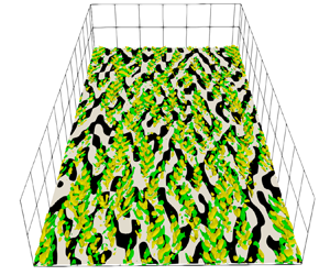
The initial optimal perturbation for $E_0= 10^{-4}$ and $T=2$ computed with respect to a turbulent snapshot extracted from the DNS at $t_0=300$ is provided in figure 2, which shows a rather complex structure. The associated premultiplied spectra are rather broad and do not show any clearly leading mode (figure 3). Nevertheless, we can note some relevant features, which are common to the optimal perturbations computed for all the considered turbulent snapshots. First, the structures are inclined against the flow (which, in figure 2, goes from left to right) as reported in all previous studies about optimal perturbations (Pringle & Kerswell 2010; Farano et al. 2015), probably to exploit the Orr's mechanism (Jiménez 2013; Encinar & Jiménez 2020). This mechanism is known to produce turbulent bursts and seems to have a role in the initiation of turbulence production at small scale allowing an energy transfer of the wall-normal energy from large to small scales, as recently shown for a minimal shear stress-driven flow model by Doohan, Willis & Hwang (2021) and by Jiao, Chernyshenko & Hwang (2022) in the case of a plane Couette flow subject to an adverse pressure gradient.

Figure 2. Optimal streamwise velocity perturbation isocontours ($\lvert \tilde {\boldsymbol{u}} \rvert =0.02, \lvert \tilde {\boldsymbol{u}} \rvert _{max}\approx 0.21$), red/blue for positive/negative.

Figure 3. Contours of the pre-multiplied spectrum of the streamwise component of the perturbation $\tilde {\boldsymbol{u}}(t_0=300)$ at $y^+=10$ (log scale). The starred point is $k_x^+=5.56\times 10^{-3}$, $k_z^+=2.22\times 10^{-2}$.

Second, and more interestingly, the perturbation forms romboidal patterns, as emphasised in figure 4 by the green lines. These lines form an angle with the streamwise direction included between $10^{\circ }$ and $20^{\circ }$. The angle varies in this range also for perturbations computed with respect to different initial snapshots. These large-scale modulations can be seen as local peaks in the spectrum. For instance, the starred point in figure 3 corresponds to an angle $\theta =\tan ^{-1}\left ( k^+_x/k^+_z \right )\approx 14^{\circ }$. We conjecture that this peculiar shape is due to the influence of the coherent structures of the unperturbed turbulent flow. Indeed, figure 5 shows the optimal perturbation along with the pre-existing coherent velocity streaks on a wall-parallel plane at $y^+=10$. To obtain the streaky pattern, we have filtered the unperturbed turbulent snapshot ($\boldsymbol {u}_u(\boldsymbol {x},t_0)$) at $t_0$. We centred the spanwise filter around the streaks’ typical spacing, $\lambda _z^+\approx 100$ ($0.03< k_z^+<0.1$, $62<\lambda _z^+<210$) and employed several intervals for the streamwise filter. In figure 5, the streaks for $0.02< k_x^+<0.05$ ($125<\lambda _x^+<314$) are shown, but a fair agreement is also found for $0.003< k_x^+<0.02$ ($314<\lambda _x^+<2095$). The local-view panels show that the optimal perturbations are positioned along the interfaces between high- and low-momentum streaks. In these regions, the shear is maximum, leading to an optimal production of energy. Moreover, local inflection points may be present which could give rise to localised instabilities (Schoppa & Hussain 2002). It is known that spanwise perturbations of a streaky base flow can induce strong (transient or asymptotic) energy growth due to the transport of the spanwise shear by the streamwise and spanwise perturbations (Hoepffner, Brandt & Henningson 2005). This mechanism of streak instability and/or transient growth has recently been shown to trigger turbulence dissipation events in a shear stress-driven flow model of near-wall turbulence involving two integral length scales of motion (Doohan et al. 2021, 2022). Thus, the structure of the optimal perturbation obtained here suggests that this streak instability/transient growth, inducing the breakdown of the streaky structures into fine scales, might be at the origin of the increase of the local dissipation within the flow.

Figure 4. Top view of the optimal streamwise velocity perturbation isocontours (as in figure 2). The green lines highlight the romboidal pattern.

Figure 5. Distribution of the optimal streamwise perturbation (shaded contours) superposed to the filtered streaks of the unperturbed flow at $t_0$ (white lines, solid for positive and dashed for negative) in the $y^+=10$ plane. The top-left panel is the whole domain, the others are details of the same figure. The streaks are obtained filtering the unperturbed flow and retaining modes between $0.02< k_x^+<0.05$ and $0.03< k_z^+<0.1$.

This point, and its connection with the generation of extreme events will be addressed in § 3.3. In the following section, the overall effect of the optimal perturbation on the flow is discussed.

3.2. Temporal evolution analysis

The evolution of two DNSs starting from the optimally perturbed and unperturbed (turbulent) flows, are now compared. The top frames of figure 6 provides snapshots extracted at the same time instant from these two simulations, showing the contours of the dissipation on a horizontal near-wall plane ($y^+=10$) at target time. In the perturbed flow (right frame), there is a much higher density of small-scale structures. This observation, together with the positioning of the perturbation along the pre-existing streaks, let us conjecture that the effect of the optimal perturbation is to destabilise the pre-existing coherent structures and engender an intense energy cascade towards the small scales. The bottom frame of the same figure shows the contours of the dissipation for a flow perturbed only in a subset of the computational domain with a clipping of the original optimal perturbation (see figure 7). The clipped perturbation is obtained multiplying the original global perturbation by a Gaussian function:

(3.3)\begin{equation} w(x,z) = \exp\left\{ - \left[ \left( \frac{x-x_c}{\ell_x/2} \right)^n + \left( \frac{z-z_c}{\ell_z/2} \right)^n \right] \right\}, \end{equation}

and subsequently projecting it on a divergence-free field. In the above equation, $\ell _x=2$ and $\ell _z=1$ are the streamwise and spanwise dimensions of the localised perturbation, respectively; $x_c$ and $z_c$ are the coordinates of the centroid of the perturbation, for which several values have been chosen; the integer $n$ is set equal to $30$. It is striking that, at target time, the flow surrounding the perturbed region is not at all modified by the perturbation and displays the same structures of the unperturbed flow. This clearly shows that the mechanisms exploited by this optimal perturbation have a local nature and that the numerous instabilities that develop in the fully perturbed flow are independent of each other.

Figure 6. Contours of the dissipation at $t=t_0+T=302$ on the $y^+=10$ plane. Top left: unperturbed flow. Top right: optimally perturbed flow. Bottom: two examples of locally perturbed flow.

Figure 7. Contours of the streamwise perturbation $\tilde {u}(\boldsymbol {x},t) = u_p(\boldsymbol {x},t) - u_u(\boldsymbol {x},t)$ for an artificially localised optimal perturbation. Top: contours of the streamwise perturbation superposed to the filtered streaks of the unperturbed flow at $t_0$ (white lines, solid for positive and dashed for negative) in the $y^+=10$ plane; the right frame shows a close-up of the left frame. Bottom: contours of the streamwise perturbation on the same plane at $t=302,305$.

Figure 8 shows the time evolution of relevant volume-averaged quantities such as the TKE ($K$) and the dissipation ($\varepsilon$), for the unperturbed and optimally perturbed flow, as well as for two other different perturbations of the undisturbed turbulent flow. In the optimally perturbed case, a peak in the volume-averaged TKE and dissipation is observed at target time. This also results in a peak of the mean wall shear stress (monitored through the friction Reynolds number on the right frame). It is useful to remark that all simulations have the same flow rate. The same figure shows that a generic, non-optimal perturbation, rescaled with the same initial energy of the optimal perturbation, does not generate any energy or dissipation peak, even if its effect on these quantities is not negligible, due to the positive Lyapunov exponents. Moreover, for comparison, we superposed to the turbulent snapshot also a monochromatic linear optimal perturbation with zero streamwise wavenumber and spanwise wavenumber equal to $10$, obtained with an optimisation around the mean flow similar to that of Del Alamo & Jimenez (2006) (see also figure 17 and the Appendix). In this case, even if a peak of TKE is indeed produced, the dissipation does not increase very much (red line in the figure). This confirms that the peak of the dissipation is given by the instability of the pre-existing structures, since the linear optimisation does not take them into account, being computed with respect to the mean flow. Indeed, even if one uses the nonlinear optimal perturbation computed with respect to a given turbulent snapshot to perturb a different snapshot, the obtained effect would not be the same (not shown).

Figure 8. Time history of the volume-averaged TKE (a,d), dissipation (b,e) and friction Reynolds number (c,f). Four flows are compared: the optimally perturbed flow (green line); the unperturbed flow (dashed black line); the flow perturbed by a non-optimal perturbation (blue line); the flow perturbed by a linear optimal perturbation with same initial energy (red line). The top line refers to the initial snapshot $t_0=300$, whereas the bottom line refers to $t_0=360$.

The peak of turbulence intensity cannot be sustained by the flow because the background turbulence is statistically stable. Therefore, after the target time, there is a relaxation towards the unperturbed flow. The flow comes back to the statistically-steady turbulent state after $\Delta T_R \approx 15$ ($\Delta T_R^+ \approx 174$). We have verified that the long time statistics of the relaxed flow are the same of the reference DNS. Finally, it is noteworthy that this behaviour is independent of the initial unperturbed snapshot chosen at $t_0$. We have recomputed the optimals and their evolutions for several snapshots and they always gave the same qualitative behaviour, as can be seen in figure 8(d–f), where the optimal perturbation is obtained for a turbulent snapshot extracted from the unperturbed DNS at $t_0=360$.

It is not easy to identify the mechanism responsible of this extreme increase of dissipation since, as we already remarked, the initial perturbation is complex and probably exploits more than one mechanism. However, here we attempt to identify the effect of the two main mechanisms of turbulent production in the channel flow: the lift-up effect (Landahl 1980) and Orr's mechanism (Orr 1907). While for the former the mean shear transport occurs in the $y$–$z$ plane, being due to streamwise-independent vortices, for the latter the production mechanism acts on the $x$–$y$ plane (Jiménez 2013). Thus, averaging the turbulent coherent structures in the streamwise, and in the spanwise directions, we can define a lift-up-like production and an Orr-like production, respectively:

(3.4a)$$\begin{gather} \mathcal{P}_{lu}(y,z,t) =-\left \langle u' \right \rangle_x \left \langle v' \right \rangle_x \frac{{\rm d}\bar{U}}{{\rm d}y}, \end{gather}$$

(3.4b)$$\begin{gather}\mathcal{P}_{Orr}(x,y,t) =-\left \langle u' \right \rangle_z \left \langle v' \right \rangle_z \frac{{\rm d}\bar{U}}{{\rm d}y}, \end{gather}$$

with $\bar {U}$ the mean turbulent profile and $\left \langle {\cdot } \right \rangle _x$, $\left \langle {\cdot } \right \rangle _z$ denoting the streamwise and spanwise average, respectively, where the prime indicates turbulent fluctuations with respect to the mean flow, thus comprising the optimal perturbation. Their capability of capturing the effect of streak-like perturbations and Orr-like perturbations is verified in the Appendix.

Figure 9 shows the time evolution of these production terms averaged along the free wall-parallel direction for the optimally perturbed (solid lines) and the unperturbed (dashed lines) flow. One can see that the averaged lift-up-like production shows a peak at several wall-normal distances: the perturbation initially produces energy near the wall ($y^+=10$, where the mean shear is maximum) and then reaches the upper layers below $y^+=90$. Instead, a relevant effect on the Orr-like production can be observed only in the near-wall layer ($y^+=10$). Note also that the Orr-like production is almost two orders of magnitude smaller than the lift-up production term and has a negative average value. Nevertheless, a peak in the curve of Orr-like production at $y^+=10$ can be observed for the perturbed flow. Comparing this peak with the corresponding peak in lift-up-like production in terms of relative gain (value of the peak of the perturbed production minus the production of the unperturbed one at the same time, divided by the value for the unperturbed flow), it can be inferred that both the mechanisms give an important contribution to the overall production. The peak in the Orr-like production is clearly linked to the backward inclination of the optimal perturbations, whereas the reason behind the peak in the lift-up-like production is better clarified by figure 10. This figure shows at times $t\geqslant t_0$ (from top to bottom) the generation of intense positive-sign streaks in the near-wall region, induced by an increased streamwise vorticity, absent in the unperturbed flow. The intensified streaks increase the wall friction in the perturbed flow and consequently the energy extracted from the mean flow through wall friction, which is transformed in an increase of dissipation.

Figure 9. Time evolution of the turbulent split production on different horizontal planes. (a) Lift-up-like production $\left \langle \mathcal {P}_{lu} \right \rangle _z$. (b) Orr-like production $\left \langle \mathcal {P}_{Orr} \right \rangle _x$. Solid lines are the optimally perturbed flow, dashed lines the unperturbed flow.

Figure 10. Time evolution of the flow averaged along the streamwise direction: isocontours of the streamwise velocity component and arrows for the transverse components. From top to bottom $t=[t_0, t_0+1, t_0+2, t_0+5]$. From left to right: perturbed flow, unperturbed flow, perturbation. For the first two columns the streamwise component refers to the turbulent fluctuation, i.e. the instantaneous velocity minus the turbulent mean profile.

These observations are consistent with those of recent works showing that the Orr-like and lift-up-like mechanisms coexist for perturbations having non-zero wavenumbers in both wall-parallel directions as none of the related terms vanish (Jiao, Hwang & Chernyshenko 2021), and that the Orr mechanism is able to energise the lift-up effect sustaining the wall cycle (Doohan et al. 2021). Thus, a sharp distinction between these two mechanisms cannot be made. However, a further insight can be gained looking at the spacetime plot of these production terms. Figure 11 shows that the perturbation increases the production in the regions where the undisturbed flow is characterised by local production peaks. This is directly linked to our previous remarks on the positioning of the perturbation over the pre-existing coherent structures. Again, it appears that the perturbation exploits the pre-existing structures and enhances their turbulent production. Moreover, the close-ups in figure 5 show that the optimal perturbations are located in the interface region between low- and high- momentum streaks, and are mostly characterised by a varicose symmetry with respect to this interface. This suggests the presence of a varicose instability of the streaks, which might be enhanced by the strengthening of the streaks due to the lift-up-like mechanism.

Figure 11. Spacetime plots of the turbulent split production. Solid black lines are the baseflow production contours (solid for positive values, dashed for negative) while shaded contours are the increment due to the perturbation ($\mathcal {P}_{lu/Orr}^p-\mathcal {P}_{lu/Orr}^u$): (a,c) $y^+=10$ plane; (b,d) $y^+=30$ plane; (a,b) lift-up-like production $\mathcal {P}_{lu}$; (c,d) Orr-like production $\mathcal {P}_{Orr}$.

To investigate whether an exponential instability is involved in these dissipative events, the time evolution of the optimal perturbation energy is shown in figure 12 for three different realisations (solid lines). In all cases, in the first time instants, the perturbation is amplified exponentially of approximately one order of magnitude in energy. This is not true for a generic non-optimal perturbation (see the blue dashed line in the figures), which grows much more slowly than the optimal and does not have relevant effects on the dissipation. This significantly supports the idea that the optimal perturbation is exploiting an exponential instability of the streaks. Moreover, due to the spatial distribution of the disturbances with respect to the streaks, this instability appears mostly of varicose type.

Figure 12. (a,b) Time evolution of the perturbation energy $1/2\left \langle \tilde {\boldsymbol{u}}, \tilde {\boldsymbol{u}} \right \rangle$ for different realisations of the perturbed flow. The dashed blue line is the evolution for a flow perturbed with a random non-optimal perturbation. (c,d) Time evolution of the individual perturbation energy budgets $1/2\left \langle \tilde {u}^2 \right \rangle$, $1/2\left \langle \tilde {v}^2 \right \rangle$ and $1/2\left \langle \tilde {w}^2 \right \rangle$ (colours as in top panels). The right panels are the dashed black rectangles magnified. The growth rate correspondent to the dashed black line in the top right panel is $\approx 3.69 U_b/h$ for the energy, i.e. ${\approx }1.84 U_b/h$ for the perturbation amplitude.

It is now worth investigating whether the optimal perturbation actually increases the number of extreme events in the flow, or it rather leads to an increase of the mean dissipation. Towards this aim, the local turbulent dissipation is considered

(3.5a,b)\begin{equation} \varepsilon = 2\nu s'_{ij}s'_{ij}, \quad s'_{ij}=\frac{1}{2}\left ( \frac{\partial{u'_i}}{\partial{x_j}}+\frac{\partial{u'_j}}{\partial{x_i}} \right ), \end{equation}

$\boldsymbol{u}'$ being the turbulent fluctuation. The p.d.f. of the normalised dissipation is computed on a given wall-parallel plane. Because extreme dissipative events are rare events, one needs to compute accurately the tail of the p.d.f. up to at least $20$ times the standard deviation. To achieve this target, one simulation of the perturbed flow is not sufficient because the transient effect of the perturbation is quite short. For this reason, we compute an ensemble of optimal perturbations with respect to eight snapshots equispaced in time extracted from the reference DNS and the corresponding ensemble of short evolutions (realisations). The dissipation is sampled on the given horizontal plane with a temporal timestep $\Delta t = 0.2$ ($\Delta t^+ \approx 2.3$) and its normalised value with respect to the standard deviation, $std(\varepsilon )$, is plotted on a p.d.f. graph in figure 13. One can see that the perturbed flow shows an increased tail, indicating a higher density of extreme events. This feature is observed on the near-wall planes at $y^+=10$ and $y^+=30$, whereas the flow near the channel centreline ($y^+>90$) remains quasi-unperturbed (not shown). The same figure shows that the linear optimal perturbation (red curve) does not produce any increment of the p.d.f. tail, i.e. it does not bring to the formation of more extreme events, despite increasing the volume-averaged dissipation. This is true also for the nonlinear optimal perturbation computed using the perturbation energy as objective function, or for much longer target times (not shown).

Figure 13. Probability density function of the local dissipation normalised with the respective standard deviation for the optimally perturbed flow (solid green line) and the unperturbed flow (dashed black): (a) $y^+=10$ plane; (b) $y^+=30$ plane. The solid red line is for the flow perturbed with a linear optimal perturbation.

It is interesting to investigate the behaviour of the nonlinear optimal perturbation in the phase space and, in particular, to address the question whether the optimally perturbed flow belongs to the turbulent attractor. Indeed, Blonigan et al. (2019) constructed their optimal perturbation combining POD modes of the reference turbulent flow in order to constrain it inside the turbulent attractor, ensuring that it would be highly probable or realistic. Despite the differences between our study and their approach (namely, they searched for an optimal turbulent field, not a small perturbation to a pre-existing turbulent field), whether the optimal flow structures may be representative of precursors of real extreme events represents an important issue concerning the physical validity of the present results. Indeed, the optimal peaks of TKE and of dissipation appear too strong to be realistic. In fact, figure 14(a) shows on a $K - \varepsilon$ projection of the phase space that the trajectory of the flow perturbed with the optimal perturbation resides out of the attractor already at the initial time (the starting point is starred in the figure), continues its excursion far away from it and finally falls back into the attractor. However, one has to consider that this projection of the phase space makes use of integral quantities. The fact that the optimal perturbation occupies the whole domain and induces many ‘synchronised’ extreme events (while realistic extreme events are local, small-scale and not synchronised) is a possible cause of this non-realistic increase of these integral quantities. On the other hand, in a real flow the optimal mechanisms may be triggered locally, providing realistic values of the integral quantities such as dissipation and TKE, and thus being representative of a realistic extreme event evolving inside the turbulent attractor.

Figure 14. (a) Turbulent attractor projected on the TKE–dissipation plane: reference DNS (solid grey line), optimally perturbed flow (solid blue) and locally perturbed flows (solid black). (b) Dissipation p.d.f. sampled on the perturbed zone in the locally perturbed flows (solid green line) and on the corresponding points in the unperturbed flow (dashed black) on the $y^+=10$ plane.

To investigate in detail this issue, a series of simulations initialised with the optimal perturbation artificially localised in different places of the domain is run for each of the eight realisations used before for the p.d.f. In particular, for each of these considered initial turbulent snapshots, the domain was divided in $36$ rectangles having dimension $\ell _x=2$, $\ell _z=1$ and, as explained previously, the portion of the optimal perturbation corresponding to each of these rectangles was used to obtain a locally perturbed flow. In each of these simulation, the perturbed zone was tracked in time taking into account the local mean advection velocity (as done by Hack & Schmidt (2021)) and the dissipation was sampled inside it, i.e. in the dashed rectangle shown in figure 7. The ensemble of the dissipation sampled in this way in each of the locally perturbed flow, constitutes the statistical sample used for the p.d.f. shown in figure 14. In figure 14(a) one can observe, in the $K - \varepsilon$ projection of the phase space, that each of this locally perturbed flows (unlike the globally perturbed one) remains within the turbulent attractor. Moreover, the right panel of the figure shows that, even when the optimal perturbation is sampled locally, the p.d.f. of the dissipation has the same increased tail of the fully perturbed flow.

Therefore, the fully perturbed flow does not reside in the projection of the turbulent attractor because the bursting mechanism is triggered everywhere at the same time. On the other hand, this is not true for locally perturbed flows, even if the perturbation is still effective in producing extreme events. In any case, it must be remarked that this is a low-dimensional projection of the attractor. Hence, this analysis alone does not prove that the locally perturbed flow is equivalent to a naturally bursting flow. This will be better investigated by means of the conditional POD analysis in § 3.3.

In the next section it will be shown that the perturbed and the unperturbed flows share the same local mechanisms during an extreme event.

3.3. POD analysis

The aim of this section is twofold: (i) to show that, locally, the mechanisms leading to an optimal dissipation in a turbulent flow are representative of those observed during the generation of extreme events in a turbulent flow; (ii) to show that extreme events happen at the interface between a positive and a negative streamwise velocity streak, exactly where the perturbation was placed by the optimisation (figure 5). For this purpose, we use the conditional spatiotemporal POD analysis proposed by Schmidt & Schmid (2019), already used for the case of the turbulent channel flow by Hack & Schmidt (2021). Following these works, extreme events are defined as local spatiotemporal dissipation peaks. In particular, Hack & Schmidt (2021) considered the 99.9th percentile of the most intense events in the dissipation of TKE, corresponding about to 20–30 times the local mean dissipation. However, our Reynolds number is significantly smaller than that used by Hack & Schmidt (2021) ($Re_{\tau }=180$ versus $2000$), leading to a much smaller number of events, which are statistically characterised by a lower intensity. For this reason, a lower threshold has been chosen equal to 10 times the local mean dissipation. The velocity field is sampled around each extreme event in a box having spatial dimension $\ell _x^+\times \ell _y^+\times \ell _z^+\approx 785\times 75\times 320$ comparable with that employed by Hack & Schmidt (2021). Moreover, the field is sampled at two instants of time before the dissipation peak and two instants of time after the peak. The spacing between these instants of time is $\Delta t_{POD} = 1.0$ in global units which corresponds to $\Delta t^+_{POD}\approx 11.7$ in wall units. The set of these five velocity fields constitutes a snapshot for the conditional space–time POD. Note that the events are sampled as they appear in the flow, i.e. randomly in space and time. Before performing the POD, the velocity field has been split in a symmetric and antisymmetric part with respect to the $\tilde {z}$ axis:

(3.6a,b)\begin{align} \boldsymbol{u}_S = \tfrac{1}{2} \begin{bmatrix} u(\tilde{x},\tilde{y},\tilde{z},\tilde{t}) + u(\tilde{x},\tilde{y},-\tilde{z},\tilde{t}) \\ v(\tilde{x},\tilde{y},\tilde{z},\tilde{t}) + v(\tilde{x},\tilde{y},-\tilde{z},\tilde{t}) \\ w(\tilde{x},\tilde{y},\tilde{z},\tilde{t}) - w(\tilde{x},\tilde{y},-\tilde{z},\tilde{t}) \end{bmatrix},\quad \boldsymbol{u}_A = \tfrac{1}{2} \begin{bmatrix} u(\tilde{x},\tilde{y},\tilde{z},\tilde{t}) - u(\tilde{x},\tilde{y},-\tilde{z},\tilde{t}) \\ v(\tilde{x},\tilde{y},\tilde{z},\tilde{t}) - v(\tilde{x},\tilde{y},-\tilde{z},\tilde{t}) \\ w(\tilde{x},\tilde{y},\tilde{z},\tilde{t}) + w(\tilde{x},\tilde{y},-\tilde{z},\tilde{t}) \\ \end{bmatrix}, \end{align}

where $\tilde {x}$, $\tilde {y}$, $\tilde {z}$ and $\tilde {t}$ denote the spatiotemporal reference frame whose origin coincides with the event location.

The following analysis refers to events sampled in the $y^+=30$ plane, the results in other near-wall planes being similar.

For the unperturbed flow, for which a long DNS is available, up to $2000$ snapshots were used. For the optimally perturbed flow, the ensemble of realisations used for computing the dissipation p.d.f. has been employed, which comprises $950$ snapshots. Taking the unperturbed case as a reference, it was possible to verify that there is a negligible difference between the modes obtained with $1000$ and $2000$ snapshots. Thus, both POD analyses were performed using ${\approx }1000$ snapshots. Note that in this conditional POD the underlying expected value operator is not temporal averaging but ensemble averaging (Berkooz, Holmes & Lumley 1993; Schmidt & Schmid 2019), therefore the approach is consistent.

Figure 15 shows that the distribution of the energy among the modes, given by the eigenvalues of the correlation matrix, is comparable in the perturbed and in the unperturbed cases. The same is true for the subdivision of energy between the symmetric and the antisymmetric parts: $51.4\,\%$ versus $48.6\,\%$, respectively, in the optimally perturbed case and $50.8\,\%$ versus $49.2\,\%$ in the unperturbed case. The results agree quite well with those of Hack & Schmidt (2021), although they found a stronger unbalance in favour of the symmetric part (${\approx }58\,\%$ versus $42\,\%$). This discrepancy may be due to the very different Reynolds numbers.

Figure 15. Distribution of the 30 leading eigenvalues of the POD. (a) Unperturbed flow. (b) Optimally perturbed flow.

Figure 16 provides the comparison of the leading POD modes of the extreme events generated in the optimally perturbed flow and in the undisturbed flow. The topology of the structures is exactly the same: the antisymmetric mode (top frames) is made of two intense streaks of opposite sign approaching each other at $y^+=30$ while the symmetric mode in the transverse plane (middle frames) shows a three lobe structure encircling a streak of opposite sign; lastly, the shear layer of the symmetric mode is inclined of the same angle with respect to the streamwise direction (bottom frames). The slight differences between the modes are due to an intrinsic variability of the turbulent flow in which these events are immersed, as confirmed by performing the conditional POD on a different set of turbulent snapshots. The comparison is very good also for instants of time before and after the peak, which are not shown for brevity. Ultimately, the optimal perturbation is found to reproduce very accurately the local mechanism behind the generation of extreme events in a turbulent flow. It exploits the high shear at the interface region between coherent low- and high-momentum regions to break down the larger structures and drive energy to small scales. The last statement further corroborates the hypothesis of Hack & Schmidt (2021) that links streak instability and the emergence of extreme dissipation in the channel flow. Thus, the local structure of the initial optimal perturbation can be seen as a precursor of extreme events.

Figure 16. Leading POD modes of the extreme events: streamwise fluctuation contours. From top to bottom: transverse view of the leading antisymmetric mode, transverse view of the leading symmetric mode, longitudinal view of the leading symmetric mode (the longitudinal view of the antisymmetric mode is not relevant). (a,c,e) Unperturbed flow. (b,d,f) Optimally perturbed flow.

4. Conclusion

Turbulent flows are characterised by intermittency at small scales consisting of the alternation of long space–time events of weak fluctuation intensity with short events of high intensity, known as extreme events, with gradients increasing by orders of magnitude. In this work, in order to investigate the mechanisms of formation of extreme events, precursors of large dissipative events in the turbulent channel flow at $Re_{\tau } = 180$ are looked for. To this purpose, the nonlinear direct-adjoint optimisation procedure presented by Farano et al. (2017) is extended to compute an optimally dissipative perturbation of a generic three-dimensional turbulent-flow snapshot. The optimisation problem is formulated using the turbulent dissipation as objective function and imposing a short target time, typical of extreme events.

The application of the optimisation procedure to a turbulent flow has been successful and, in all cases, a satisfactory convergence has been achieved. The results show that the optimal perturbation is localised in the near-wall region and displays the upstream tilting characteristic of Orr's mechanism. Interestingly, it is found that the perturbation is positioned along the pre-existing flow structures of the turbulent snapshot with respect to which it was computed. In particular, it is placed at the interface between a positive and a negative streamwise velocity streak, i.e. in the regions of highest shear, where the perturbation may consistently exploit the lift-up mechanism. Moreover, in the near-wall region, also the Orr mechanism appears to be involved.

Comparing the evolution of the perturbed flow to that of the unperturbed flow, one can observe that the perturbation leads to: (i) a sudden breakdown of the pre-existing structures; (ii) a strong peak in the global turbulent dissipation; (iii) a growth of the tail in the p.d.f. of the dissipation indicating a higher number of extreme events. It is found that the optimal perturbation, despite an intrinsic multimodal nature, grows exponentially during the first phase of its evolution reflecting the existence of a secondary modal instability of the streaks in the very first moments. This fact strongly corroborates the idea of a connection between extreme events and exponential instability of turbulent structures. Moreover, the perturbation also causes the formation of strong positive-sign streaks near the wall through a modified lift-up effect. It is argued that this mechanism is able to feed the energy cascade responsible for the extreme events. The robustness and statistical relevance of this behaviour is assessed repeating the numerical experiment using different initial snapshots (realisations). Most importantly, further computations show that the instability mechanism has a local nature, namely, when only a portion of the domain is optimally perturbed the surrounding structures are not affected and the flow globally resides in the turbulent attractor. Even in this case, an increase of the tail of the p.d.f. distribution of the dissipation is observed for the local region interested by the perturbation.

Finally, a conditional POD analysis has been performed on the different realisations of the optimisation and on the unperturbed turbulent flow, to show that the optimal mechanisms are indeed representative of those occurring during extreme events in a turbulent channel flow, i.e. that the optimal perturbation captures the physically relevant mechanisms inducing extreme events.

Therefore, a large number of extreme events having the same local structure of naturally occurring ones are generated in the optimally perturbed flow. Different mechanisms are at play during this process: the high shear present at the interface region between coherent low- and high-momentum regions is exploited to break down the larger structures and drive energy to small scales. This energy cascade is fed by an enhanced lift-up effect that produces intense streaks near the wall, causing a stronger wall friction. This process, which is most efficiently triggered by the optimal perturbation, appears to be the same of that observed in naturally occurring extreme events. Thus, the optimal perturbation at initial time can be considered as a precursor of extreme events.

References

Adrian, R.J. 2007 Hairpin vortex organization in wall turbulence. Phys. Fluids 19 (4), 041301.CrossRefGoogle Scholar
Andersson, P., Brandt, L., Bottaro, A. & Henningson, D.S. 2001 On the breakdown of boundary layer streaks. J. Fluid Mech. 428, 2960.CrossRefGoogle Scholar
Berkooz, G., Holmes, P. & Lumley, J.L. 1993 The proper orthogonal decomposition in the analysis of turbulent flows. Annu. Rev. Fluid Mech. 25 (1), 539575.CrossRefGoogle Scholar
Bernardini, M. & Pirozzoli, S. 2011 Inner/outer layer interactions in turbulent boundary layers: a refined measure for the large-scale amplitude modulation mechanism. Phys. Fluids 23 (6), 061701.CrossRefGoogle Scholar
Blonigan, P.J., Farazmand, M. & Sapsis, T.P. 2019 Are extreme dissipation events predictable in turbulent fluid flows? Phys. Rev. Fluids 4 (4), 044606.CrossRefGoogle Scholar
Boffetta, G., Giuliani, P., Paladin, G. & Vulpiani, A. 1998 An extension of the Lyapunov analysis for the predictability problem. J. Atmos. Sci. 55 (23), 34093416.2.0.CO;2>CrossRefGoogle Scholar
Brandt, L., Schlatter, P. & Henningson, D.S. 2004 Transition in boundary layers subject to free-stream turbulence. J. Fluid Mech. 517, 167198.CrossRefGoogle Scholar
Buaria, D., Pumir, A. & Bodenschatz, E. 2020 Self-attenuation of extreme events in Navier–Stokes turbulence. Nat. Commun. 11 (1), 5852.CrossRefGoogle ScholarPubMed
Butler, K. & Farrell, B. 1992 Three-dimensional optimal perturbations in viscous shear flow. Phys. Fluids A 4 (8), 16371650.CrossRefGoogle Scholar
Butler, K.M. & Farrell, B.F. 1993 Optimal perturbations and streak spacing in wall-bounded turbulent shear flow. Phys. Fluids A 5 (3), 774777.CrossRefGoogle Scholar
Cassinelli, A., de Giovanetti, M. & Hwang, Y. 2017 Streak instability in near-wall turbulence revisited. J. Turbul. 18 (5), 443464.CrossRefGoogle Scholar
Cherubini, S. & De Palma, P. 2013 Nonlinear optimal perturbations in a couette flow: bursting and transition. J. Fluid Mech. 716, 251279.CrossRefGoogle Scholar
Cherubini, S. & De Palma, P. 2015 Minimal-energy perturbations rapidly approaching the edge state in Couette flow. J. Fluid Mech. 764, 572598.CrossRefGoogle Scholar
Cherubini, S., De Palma, P. & Robinet, J.-C. 2015 Nonlinear optimals in the asymptotic suction boundary layer: transition thresholds and symmetry breaking. Phys. Fluids 27 (3), 034108.CrossRefGoogle Scholar
Cherubini, S., De Palma, P., Robinet, J.-C. & Bottaro, A. 2010 Rapid path to transition via nonlinear localized optimal perturbations in a boundary-layer flow. Phys. Rev. E 82 (6), 066302.CrossRefGoogle Scholar
Cossu, C. & Hwang, Y. 2017 Self-sustaining processes at all scales in wall-bounded turbulent shear flows. Phil. Trans. R. Soc. Lond. A 375 (2089), 20160088.Google ScholarPubMed
Cossu, C., Pujals, G. & Depardon, S. 2009 Optimal transient growth and very large–scale structures in turbulent boundary layers. J. Fluid Mech. 619, 7994.CrossRefGoogle Scholar
Del Alamo, J.C. & Jimenez, J. 2006 Linear energy amplification in turbulent channels. J. Fluid Mech. 559, 205213.CrossRefGoogle Scholar
Doohan, P., Bengana, Y., Yang, Q., Willis, A.P. & Hwang, Y. 2022 The state space and travelling-wave solutions in two-scale wall-bounded turbulence. J. Fluid Mech. 947, A41.CrossRefGoogle Scholar
Doohan, P., Willis, A.P. & Hwang, Y. 2021 Minimal multi-scale dynamics of near-wall turbulence. J. Fluid Mech. 913, A8.CrossRefGoogle Scholar
Duguet, Y., Monokrousos, A., Brandt, L. & Henningson, D.S. 2013 Minimal transition thresholds in plane Couette flow. Phys. Fluids 25 (8), 084103.CrossRefGoogle Scholar
Eaves, T.S. & Caulfield, C.P. 2015 Disruption of states by a stable stratification. J. Fluid Mech. 784, 548564.CrossRefGoogle Scholar
Encinar, M.P. & Jiménez, J. 2020 Momentum transfer by linearised eddies in turbulent channel flows. J. Fluid Mech. 895, A23.CrossRefGoogle Scholar
Farano, M., Cherubini, S., De Palma, P. & Robinet, J.-C. 2018 Nonlinear optimal large-scale structures in turbulent channel flow. Eur. J. Mech. (B/Fluids) 72, 7486.CrossRefGoogle Scholar
Farano, M., Cherubini, S., Robinet, J.-C. & De Palma, P. 2015 Hairpin-like optimal perturbations in plane Poiseuille flow. J. Fluid Mech. 775, R2.CrossRefGoogle Scholar
Farano, M., Cherubini, S., Robinet, J.-C. & De Palma, P. 2017 Optimal bursts in turbulent channel flow. J. Fluid Mech. 817, 3560.CrossRefGoogle Scholar
Foures, D.P.G., Caulfield, C.P. & Schmid, P.J. 2013 Localization of flow structures using norm optimization. J. Fluid Mech. 729, 672701.CrossRefGoogle Scholar
Gibson, J., et al. 2021 Channelflow2.0. Available at: https://www.channelflow.ch/.Google Scholar
Hack, M.J.P. & Moin, P. 2018 Coherent instability in wall-bounded shear. J. Fluid Mech. 844, 917955.CrossRefGoogle Scholar
Hack, M.J.P. & Schmidt, O.T. 2021 Extreme events in wall turbulence. J. Fluid Mech. 907, A9.CrossRefGoogle Scholar
Hack, M.J.P. & Zaki, T.A. 2014 Streak instabilities in boundary layers beneath free-stream turbulence. J. Fluid Mech. 741, 280315.CrossRefGoogle Scholar
Hall, P. & Smith, F.T. 1991 On strongly nonlinear vortex/wave interactions in boundary-layer transition. J. Fluid Mech. 227, 641666.CrossRefGoogle Scholar
Hamilton, J.M., Kim, J. & Waleffe, F. 1995 Regeneration mechanisms of near-wall turbulence structures. J. Fluid Mech. 287, 317348.CrossRefGoogle Scholar
Head, M.R. & Bandyopadhyay, P. 1981 New aspects of turbulent boundary-layer structure. J. Fluid Mech. 107, 297338.CrossRefGoogle Scholar
Hoepffner, J., Brandt, L. & Henningson, D.S. 2005 Transient growth on boundary layer streaks. J. Fluid Mech. 537, 91100.CrossRefGoogle Scholar
Hwang, Y. 2015 Statistical structure of self-sustaining attached eddies in turbulent channel flow. J. Fluid Mech. 767, 254289.CrossRefGoogle Scholar
Hwang, Y. & Bengana, Y. 2016 Self-sustaining process of minimal attached eddies in turbulent channel flow. J. Fluid Mech. 795, 708738.CrossRefGoogle Scholar
Hwang, Y. & Cossu, C. 2010 Self-sustained process at large scales in turbulent channel flow. Phys. Rev. Lett. 105 (4), 044505.CrossRefGoogle ScholarPubMed
Jahanbakhshi, R. & Zaki, T.A. 2019 Nonlinearly most dangerous disturbance for high-speed boundary-layer transition. J. Fluid Mech. 876, 87121.CrossRefGoogle Scholar
Jiao, Y., Chernyshenko, S.I. & Hwang, Y. 2022 A driving mechanism of near-wall turbulence subject to adverse pressure gradient in a plane Couette flow. J. Fluid Mech. 941, A37.CrossRefGoogle Scholar
Jiao, Y., Hwang, Y. & Chernyshenko, S.I. 2021 Orr mechanism in transition of parallel shear flow. Phys. Rev. Fluids 6, 023902.CrossRefGoogle Scholar
Jiménez, J. 2013 How linear is wall-bounded turbulence? Phys. Fluids 25 (11), 110814.CrossRefGoogle Scholar
Jiménez, J. 2018 Coherent structures in wall-bounded turbulence. J. Fluid Mech. 842, P1.CrossRefGoogle Scholar
Jimenéz, J. 2020 Monte Carlo science. J. Turbul. 21, 544566.CrossRefGoogle Scholar
Jiménez, J. & Pinelli, A. 1999 The autonomous cycle of near-wall turbulence. J. Fluid Mech. 389, 335359.CrossRefGoogle Scholar
Kerswell, R.R. 2018 Nonlinear nonmodal stability theory. Annu. Rev. Fluid Mech. 50, 319345.CrossRefGoogle Scholar
Kim, H.T., Kline, S.J. & Reynolds, W.C. 1971 The production of turbulence near a smooth wall in a turbulent boundary layer. J. Fluid Mech. 50 (1), 133160.CrossRefGoogle Scholar
Kim, J., Moin, P. & Moser, R. 1987 Turbulence statistics in fully developed channel flow at low Reynolds number. J. Fluid Mech. 177, 133166.CrossRefGoogle Scholar
Kline, S.J., Reynolds, W.C., Schraub, F.A. & Runstadler, P.W. 1967 The structure of turbulent boundary layers. J. Fluid Mech. 30 (4), 741773.CrossRefGoogle Scholar
Landahl, M.T. 1980 A note on an algebraic instability of inviscid parallel shear flows. J. Fluid Mech. 98 (2), 243251.CrossRefGoogle Scholar
Lozano-Durán, A., Flores, O. & Jiménez, J. 2012 The three-dimensional structure of momentum transfer in turbulent channels. J. Fluid Mech. 694, 100130.CrossRefGoogle Scholar
Monokrousos, A., Bottaro, A., Brandt, L., Di Vita, A. & Henningson, D.S. 2011 Nonequilibrium thermodynamics and the optimal path to turbulence in shear flows. Phys. Rev. Lett. 106 (13), 134502.CrossRefGoogle ScholarPubMed
Morrison, J.F., Tsai, J.F. & Bradshaw, P. 1988 Conditional-sampling schemes for turbulent flow, based on the variable-interval time averaging (VITA) algorithm. Exp. Fluids 7, 173186.CrossRefGoogle Scholar
Nikitin, N. 2018 Characteristics of the leading Lyapunov vector in a turbulent channel flow. J. Fluid Mech. 849, 942967.CrossRefGoogle Scholar
Orr, W.M.F. 1907 The stability or instability of the steady motions of a perfect liquid and of a viscous liquid. Part II: a viscous liquid. Proc. R. Ir. Acad. Sec. A: Math. Phys. Sci. 27, 69138.Google Scholar
Pralits, J.O., Bottaro, A. & Cherubini, S. 2015 Weakly nonlinear optimal perturbations. J. Fluid Mech. 785, 135151.CrossRefGoogle Scholar
Pringle, C.C.T. & Kerswell, R.R. 2010 Using nonlinear transient growth to construct the minimal seed for shear flow turbulence. Phys. Rev. Lett. 105 (15), 154502.CrossRefGoogle ScholarPubMed
Pringle, C.C.T., Willis, A.P. & Kerswell, R.R. 2012 Minimal seeds for shear flow turbulence: using nonlinear transient growth to touch the edge of chaos. J. Fluid Mech. 702, 415443.CrossRefGoogle Scholar
Pujals, G., García-Villalba, M., Cossu, C. & Depardon, S. 2009 A note on optimal transient growth in turbulent channel flows. Phys. Fluids 21 (1), 015109.CrossRefGoogle Scholar
Rabin, S.M.E., Caulfield, C.P. & Kerswell, R.R. 2012 Triggering turbulence efficiently in plane Couette flow. J. Fluid Mech. 712, 244272.CrossRefGoogle Scholar
Rabin, S.M.E., Caulfield, C.P. & Kerswell, R.R. 2014 Designing a more nonlinearly stable laminar flow via boundary manipulation. J. Fluid Mech. 738, R1.CrossRefGoogle Scholar
Reddy, S.C. & Henningson, D.S. 1993 Energy growth in viscous channel flows. J. Fluid Mech. 252, 209238.CrossRefGoogle Scholar
Sapsis, T.P. 2021 Statistics of extreme events in fluid flows and waves. Annu. Rev. Fluid Mech. 53, 85111.CrossRefGoogle Scholar
Saw, E.-W., Kuzzay, D., Faranda, D., Guittonneau, A., Daviaud, F., Wiertel-Gasquet, C., Padilla, V. & Dubrulle, B. 2016 Experimental characterization of extreme events of inertial dissipation in a turbulent swirling flow. Nat. Commun. 7 (1), 12466.CrossRefGoogle Scholar
Schmidt, O.T. & Schmid, P.J 2019 A conditional space–time pod formalism for intermittent and rare events: example of acoustic bursts in turbulent jets. J. Fluid Mech. 867, R2.CrossRefGoogle Scholar
Schoppa, W & Hussain, F. 2002 Coherent structure generation in near-wall turbulence. J. Fluid Mech. 453, 57108.CrossRefGoogle Scholar
Sreenivasan, K.R. & Antonia, R.A. 1997 The phenomenology of small-scale turbulence. Annu. Rev. Fluid Mech. 29 (1), 435472.CrossRefGoogle Scholar
Waleffe, F. 1997 On a self-sustaining process in shear flows. Phys. Fluids 9 (4), 883900.CrossRefGoogle Scholar
Yang, Q., Willis, A.P. & Hwang, Y. 2019 Exact coherent states of attached eddies in channel flow. J. Fluid Mech. 862, 10291059.CrossRefGoogle Scholar
Yeung, P.K., Zhai, X.M. & Sreenivasan, K.R. 2015 Extreme events in computational turbulence. Proc. Natl Acad. Sci. USA 112 (41), 1263312638.CrossRefGoogle ScholarPubMed