Hostname: page-component-745bb68f8f-5r2nc Total loading time: 0 Render date: 2025-01-27T17:44:43.257Z Has data issue: false hasContentIssue false

Modelling high-Reynolds-number effects in fully developed channel flows using a two-scale Reynolds stress model

Published online by Cambridge University Press:  28 November 2024

François Chedevergne*
Affiliation:
DMPE, ONERA, Université de Toulouse, Toulouse, France
Stefan Coroama
Affiliation:
DAAA, ONERA, Institut Polytechnique de Paris, Meudon, France
Vincent Gleize
Affiliation:
DAAA, ONERA, Institut Polytechnique de Paris, Meudon, France
Hervé Bézard
Affiliation:
DMPE, ONERA, Université de Toulouse, Toulouse, France
*
Email address for correspondence: [email protected]

Abstract

Reynolds-averaged models for solving the Navier–Stokes equations are implicitly based on Kolmogorov's theory for describing energy transfers between the different turbulent scales, which means that all the energy produced at large scales is transferred at a constant rate to the smallest turbulent scales where it is dissipated. As a result, these models use a single scale to describe the turbulence spectrum, which in cases of non-equilibrium turbulence does not provide an adequate description of the transfers actually observed. This is particularly the case for wall-bounded flows at high Reynolds numbers, such as turbulent channel flows. Taking up an approach developed by Schiestel (2007 Modeling and Simulation of Turbulent Flows, ISTE Ltd and John Wiley & Sons), which aims to define a Reynolds-averaged Navier–Stokes model transporting several scales of turbulence, a two-scale Reynolds stress model (RSM) was developed in order to take into account the interactions between the inner and outer regions of wall-bounded flows. The results obtained with the model are compared with the direct numerical simulations (DNS) of Lee & Moser (J. Fluid Mech., vol. 860, 2019, pp. 886–938) in a turbulent channel for several friction Reynolds numbers up to $Re_{\tau }=5200$, for which partial integrations in spectral space were carried out, highlighting distinct behaviours between small and large scales of turbulence. The model developed provides an accurate description of the contributions at small and large scales and thus reproduces the high-Reynolds-number effects observed in DNS data. In addition, comparisons with the DNS data served to validate a large part of the closure relations used for the various terms in the two-scale RSM.

Type
JFM Papers
Copyright
© The Author(s), 2024. Published by Cambridge University Press

1. Introduction

For equilibrium turbulence, Kolmogorov's theory implies that the energy flux cascading from large scales (LS) to small scales (SS) is equal to the dissipation rate of energy. Thus, the dissipation rate is determined entirely by the large energy-containing eddies. From this standpoint, the dissipation rate is independent of the Reynolds number, if the latter is large enough. Only the dissipation scale depends on the Reynolds number. In real situations, turbulence is evolving and not necessarily at equilibrium, so dissipation will not be equal to the energy flux coming from the energetic eddies. There is a delay in this energy transfer, which corresponds to the characteristic time it takes for a large eddy to cascade and give rise to smaller eddies. Local and non-local interactions take place in turbulent flows (Laval, Dubrulle & Nazarenko Reference Laval, Dubrulle and Nazarenko2001), which translates spectrally into possible energy transfers between remote wavenumbers. Direct transfers to immediately higher wavenumbers are the most energetic, but a small proportion of the energy can be transferred to remote wavenumbers. Inverse energy transfers, from SS to LS, can also occur.

Standard turbulence models are based on one-point closures and are therefore local models. Their great popularity is attributable to their ability to correctly predict non-homogeneous turbulent shear flows, which are those most commonly encountered in industry. However, in addition to the purely local nature of one-point closure models, these models also suffer from the single-scale assumption underlying their development. A single-scale model means that the length and time scales are linked together, through the turbulent quantities transported. This hypothesis derives directly from Kolmogorov's theory and the expected universal character of the spectrum shape. In these models, the dissipation is used to evaluate the energy-containing eddies acting at LS. The energy transfer rate is implicitly equal to the dissipation, which from a physical viewpoint is related to the smallest structures, i.e. Kolmogorov's scale. The single-scale hypothesis can therefore only represent an equilibrium turbulence.

Multi-scale models offers a framework to tackle the turbulent interactions between the different parts of a turbulent spectrum still using one-point closures. Pioneer works may be attributed to Schiestel during his PhD (Schiestel Reference Schiestel1974) and were further improved by introducing a spectrum partitioning (Hanjalić, Launder & Schiestel Reference Hanjalić, Launder and Schiestel1979). Multi-scale equations were then formally derived from partial integration of spectral equations applicable to homogeneous anisotropic turbulence (Schiestel Reference Schiestel1987). There are few concrete models based on his ideas, with the notable exception of the work of Gleize, Schiestel & Couaillier (Reference Gleize, Schiestel and Couaillier1996), Grégoire et al. (Reference Grégoire, Souffland, Gauthier and Schiestel1999) and Cadiou, Hanjalić & Stawiarski (Reference Cadiou, Hanjalić and Stawiarski2004). More recently Chaouat & Schiestel (Reference Chaouat and Schiestel2007) proved the applicability of the approach on non-isotropic non-homogeneous turbulence based on the work of Laporta & Bertoglio (Reference Laporta and Bertoglio1995) and using the hypothesis of locally constant mean velocity gradient. The partial energies and the spectral fluxes are used to define the different length scales to characterise mechanisms such as return to isotropy, dissipation and turbulent diffusion. The ratio of the partial energies or of the spectral fluxes are direct measures of the departure from the equilibrium situation. The main difficulty of this approach lies in the definition of a closure relation for the tensorial form of the spectral fluxes that derives from the partial integration of the two-point transport equations (Schiestel Reference Schiestel2007).

High-Reynolds-number wall-bounded flows are a major concern in fluid mechanics and are notoriously challenging to study both experimentally and numerically. The wall-blocking effect (Manceau & Hanjalić Reference Manceau and Hanjalić2002) creates high levels of inhomogeneity and anisotropy, making Kolmogorov's theory invalid in these areas. In the near-wall regions, with high Reynolds numbers, the turbulence spectra cannot simply be described by a constant-rate energy cascade. Wall-bounded flows are generally broken down into an inner region and an outer region, which are characterised by scale separation. The mean velocity profile then behaves logarithmically with respect to the wall distance in the overlap zone at high Reynolds numbers, with a constant and universal slope, although this last point remains controversial (Nagib & Chauhan Reference Nagib and Chauhan2008; Monkewitz Reference Monkewitz2017; Monkewitz & Nagib Reference Monkewitz and Nagib2023). SS eddies dominates near walls, whereas LS eddies dominate further out (Hutchins & Marusic Reference Hutchins and Marusic2007b). The classical description of near-wall turbulence assumes the inner region to be independent from the outer region making time-averaged normalised quantities using wall units independent of the Reynolds number. However, this view has now been proved to be erroneous and one of the most remarkable example for this is that it is now well-established (Marusic, Baars & Hutchins Reference Marusic, Baars and Hutchins2017) that the near-wall peak of the streamwise turbulence intensity depends on the Reynolds number $Re$. A secondary peak, the intensity of which depends on $Re$, also arises at LS and modulates the SS energy in the near-wall region (Marusic, Mathis & Hutchins Reference Marusic, Mathis and Hutchins2010b). At large high Reynolds numbers, i.e. when the scale separation is sufficient, the footprint of the LS is seen as a modulated boundary condition by the SS, through a change of the inner scaling as Marusic et al. (Reference Marusic, Baars and Hutchins2017) explained. High-Reynolds-number effects are well-documented in channels (Sillero, Jiménez & Moser Reference Sillero, Jiménez and Moser2013; Lee & Moser Reference Lee and Moser2015), in pipes (Ono, Furuichi & Tsuji Reference Ono, Furuichi and Tsuji2023) and in boundary layers (Vallikivi, Hultmark & Smits Reference Vallikivi, Hultmark and Smits2015; Marusic, Mathis & Hutchins Reference Marusic, Mathis and Hutchins2010a). Concerning channel flows, Lee & Moser (Reference Lee and Moser2019) applied a spectrum partitioning to their direct numerical simulations (DNS) in order to separate LS contributions from SS ones on the different terms involved in the transport equations of the Reynolds stresses. The dimensionless cut-off wavelength was set to $1000$ allowing the SS streamwise intensity to be independent of the Reynolds number. The LS counterpart is then shown to be strongly affected by $Re$.

Standard one-point closure Reynolds-averaged Navier–Stokes (RANS) models of first or second order relying on the single-scale assumption can provide only a unique prediction for the inner region, the outer region being scaled accordingly. Wall-unit quantities are all independent of the Reynolds number in the inner region, which notably results from the assumed equilibrium between production and dissipation of the turbulent kinetic energy in the logarithmic region. It is therefore pointless to hope to capture high-Reynolds-number effects with a single-scale RANS model. Nevertheless, although a model having a physically relevant predictions up to second-order moments is always desirable, single-scale models are commonly used in many wall-bounded flow applications since the effects of high Reynolds numbers are not visible on the mean flow. The main motivation for developing a model capable of handling the LS and SS contributions revealed at high Reynolds numbers comes from recent evidence of the role played by both types of contributions in boundary layers exposed to high freestream turbulence levels (Jooss et al. Reference Jooss, Li, Bracchi and Hearst2021) or adverse pressure gradients (Harun et al. Reference Harun, Monty, Mathis and Marusic2013). The framework developed in the present study for high-Reynolds-number effects, for which comprehensive DNS data can be exploited (Lee & Moser Reference Lee and Moser2019), is thus intended to serve as a basis for other important applications where single-scale models fail, even for mean flow. The objective here is to reuse the foundations of the multi-scale approach developed by Schiestel (Reference Schiestel2007) and implement it on the basis of a Reynolds stress model (RSM). The multi-scale approach is recalled in § 2 and applied to the elliptic blending Reynolds stress model (EBRSM) of Manceau (Reference Manceau2015). This model was chosen for its ability to describe the behaviour of Reynolds stresses in the near wall. It provides an excellent basis on which to develop a multi-scale model. The model is tested in § 3 against the DNS database of Lee & Moser (Reference Lee and Moser2019) and the SS and LS contributions are examined on the different terms involved in the Reynolds stress transport equations.

2. A multi-scale RSM

Let $\varphi _{ij}$ be the spherical mean of the Fourier transform of the two-point correlation tensor depending on the position $\displaystyle \boldsymbol {x}$ and the wavenumber $\kappa =\Vert \boldsymbol {\kappa } \Vert$, such that the Reynolds stress $R_{ij}$ is given by its integral:

(2.1)\begin{equation} \displaystyle R_{ij}(\boldsymbol{x}) = \int\limits_{0}^{\infty} \varphi_{ij}(\boldsymbol{x},\kappa) \,{\rm d}\kappa. \end{equation}

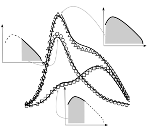
The corresponding spectrum can be split into $n+1$ slices as illustrated in figure 1. Formally, a multi-scale RSM derived from the approach proposed by Schiestel (Reference Schiestel2007) may be written for an incompressible fluid as follows:

(2.2)\begin{equation} \displaystyle \frac{{\rm D}R^{(m)}_{ij}}{{\rm D}t} = P^{(m)}_{ij}+ F^{(m-1)}_{ij}-F^{(m)}_{ij}+\varPhi^{(m)}_{ij} + D^{(m)}_{ij} - \varepsilon^{(m)}_{ij}, \end{equation}

with

(2.3)\begin{equation} \displaystyle R_{ij}^{(m)}={\overline{u'_iu'_j}}^{(m)}=\int\limits_{\kappa_{m-1}}^{\kappa_m} \varphi_{ij} \,{\rm d}\kappa. \end{equation}

The overbar symbol is used for the Reynolds-averaged quantities whereas prime is used for fluctuating quantities. Here $P^{(m)}_{ij}=-R^{(m)}_{ik}({\partial \overline {u_j}}/\partial {x_k})-R^{(m)}_{jk}({\partial \overline {u_i}}/\partial {x_k})$ is the exact production term in slice $m$, $\varPhi ^{(m)}_{ij}$ is the pressure–strain correlation corresponding to the redistribution term in the slice, ${D}^{(m)}_{ij}$ the diffusion term including the viscous diffusion, the turbulent diffusion, denoted by ${T}^{(m)}_{ij}$ in the following, and the pressure diffusion and $\varepsilon ^{(m)}_{ij}$ the dissipation associated with slice $m$. The velocity–pressure gradient correlation is here decomposed into the pressure–strain correlation $\varPhi _{ij}$ and the pressure diffusion term. The flux term $F^{(m)}_{ij}$ denotes the rate of energy transfer leaving slice $m$. Therefore, in the last slice all the outgoing energy is dissipated and $F^{(n)}_{ij}=\varepsilon ^{(n+1)}$.

Figure 1. Spectrum partitioning of the two-point correlation tensor $\varphi _{ij}$. In each slice $m$ such that $\kappa \in [{\kappa }^{(m-1)},{\kappa }^{(m)}]$, ${P}^{(m)}_{ij}$ is the corresponding production term, ${D}^{(m)}_{ij}$ the diffusion term, ${\varPhi }^{(m)}_{ij}$ the redistribution term and ${F}^{(m)}_{ij}$ the rate of transfer tensor. The one-point velocity correlation ${R}^{(m)}_{ij}$ is obtained by integration of $\varphi _{ij}$ over slice $m$.

Implicitly, the above partitioning means that any flow quantity $q$ is averaged from an extended form of the Reynolds decomposition which reads

(2.4)\begin{equation} \displaystyle q = \bar{q} + \sum_{j=1}^{n} q^{'(j)}. \end{equation}

To model the energy flux, Schiestel (Reference Schiestel2007) assumed that the slice width is given by a length scale related to the turbulent kinetic energy flux $F^{(m)}=\tfrac {1}{2}F^{(m)}_{ii}$ such that

(2.5)\begin{equation} \kappa(m)-\kappa(m-1) \propto \frac{F^{(m)}}{k^{{(m)}^{3/2}}}. \end{equation}

When deriving the $\varphi _{ij}$ equation (Schiestel Reference Schiestel2007) and then applying (2.3), it is shown that the transfer rate ${F}^{(m)}$ is composed of an inertial transfer contribution ${\mathcal {F}_t}^{(m)}$ from the energy cascade, a rapid transfer contribution ${\mathcal {F}_u}^{(m)}$ due to straining of turbulence through the action of the mean velocity gradients and a contribution due to the variations in the splitting wavenumbers, which gives

(2.6)\begin{equation} {F}^{(m)} = {\mathcal{F}_t}^{(m)} + {\mathcal{F}_u}^{(m)} - K\left(\kappa\right)\frac{\partial \kappa}{\partial t}, \end{equation}

where $K$ is the turbulent kinetic energy density in the spectral space such that ${k}^{(m)}=\int _{\kappa (m-1)}^{\kappa (m)}K \,{\rm d}\kappa$. We remark that in developed turbulent channel flows, the contribution ${\mathcal {F}_u}^{(m)}$ is zero due to homogeneity in the horizontal ($x$ and $z$) directions. From the two previous relations (2.5) and (2.6) and after a little algebra, Schiestel (Reference Schiestel2007) proves that ${F}^{(m)}$ is ruled by a transport equation of the general form:

(2.7)\begin{equation} \frac{{\rm D}F^{(m)}}{{\rm D}t} = \frac{F^{(m)}}{k^{(m)}}\left( C_1^{(m)}P^{(m)}+ C_2^{(m)}F^{(m-1)}- C_3^{(m)}F^{(m)} - C_4^{(m)}\varepsilon^{(m)}\right). \end{equation}

Finally, a formulation inspired by Rotta hypothesis is retained to assess $F_{ij}^{(m)}$:

(2.8)\begin{equation} F_{ij}^{(m)}=\frac{F^{(m)}}{k^{(m)}}\left(A^{(m)}R_{ij}^{(m)}+\frac{2}{3}\left(1-A^{(m)}\right)k^{(m)}\delta_{ij}\right), \end{equation}

with $A^{(m)}$ a constant ranging from $0$ to $1$. For slices $m$ involving large wavenumbers where isotropy is expected, $A^{(m)}$ is assumed to take a value close to zero, whereas for slices $m$ in the region of low wavenumbers, $A^{(m)}$ may reach values close to unity. More complicated attempts were also proposed by Schiestel (Reference Schiestel2007) to model the energy transfer, in particular to account for the fast transfer contribution which also causes energy redistribution among the Reynolds stress tensor components.

All previous developments are valid for free flows, without consideration of wall effects. Although some proposals were formulated by Schiestel (Reference Schiestel2007) to incorporate near-wall behaviour with ad hoc wall functions, no complete multi-scale RSM was fully derived to compute wall-bounded flows. This is one of the most challenging aspects of developing a multi-scale model, and was a stumbling block to date. For the description of wall-bounded flows with emphasis on the similarities existing in the near-wall region, physical quantities are generally made dimensionless using the kinematic viscosity $\nu$ and the friction velocity $u_{\tau }$. The sign $+$ is used in the following to denote dimensionless quantities.

To revisit the approach developed by Schiestel and implement it to capture high-Reynolds-number effects in channel flows, the spectrum is split into three parts ($n=2$, see figure 1) in analogy with the scale separation proposed by Lee & Moser (Reference Lee and Moser2019) and, thus, forming a two-scale model. The EBRSM model of Manceau (Reference Manceau2015) is considered as the base model from which the closure relations for the pressure–strain correlation and the turbulent diffusion are taken. In order to distinguish dissipation from energy transfers between spectral bands, which are mixed up in single-scale models, we slightly modify Manceau's model by decomposing dissipation into a homogeneous part $\tilde {\varepsilon }$, corresponding to the energy flux, and a near-wall inhomogeneous part $\varepsilon _w$, as is conventionally done (Jones & Launder Reference Jones and Launder1972; Gleize et al. Reference Gleize, Schiestel and Couaillier1996). Numerical tests on the EBRSM model showed the best agreement with the original model for $\varepsilon = \tilde {\varepsilon } + \varepsilon _w$, where

(2.9)\begin{equation} \varepsilon_w=\frac{2\nu k}{y^{2}}\left[\frac{1}{y^{+^{0.8}}}\tanh \left(\frac{y^+}{2.5}\right) + \left(1-\tanh \left(\frac{y^+}{2.5}\right)\right)\right], \end{equation}

which guarantees correct theoretical behaviour at the wall. In Schiestel's approach, the transfer rate $F^{(m)}$ is directly related to the spectral width of the slice. By adjusting the level of these fluxes, we can adjust the location of the cut-off in spectral space. In the analysis proposed by Lee & Moser (Reference Lee and Moser2019), the energy transfers are found to take place in the logarithmic region, well beyond the buffer layer and the viscous sublayer. This reflects the fact that the large structures transfer energy to the small structures and that the large structures are essentially located further from the wall than the small ones (Hutchins & Marusic Reference Hutchins and Marusic2007b). Hence, in order to position the spectral cut-off for a wavelength $\lambda ^+=1000$ as Lee and Moser did, the damping functions associated with the two transported scales are judiciously adjusted. In the EBRSM model, the damping is controlled by a blending function derived from an elliptic equation. In our two-scale model, the coefficients governing each of the elliptical equations associated with the transported scales can be used to adjust the position of the spectral cut-off.

Lee & Moser (Reference Lee and Moser2019) showed that partitioning the spectral space into a LS contribution and a SS contribution with a cut-off wavenumber fixed at $\lambda ^+=1000$ is an appropriate choice for describing the near-wall behaviour of channel flows. This corroborates previous observations on wall flows where two distinct turbulent scales can be identified, one characterising the near-wall cycle (Jiménez & Pinelli Reference Jiménez and Pinelli1999) and a second characterising the ‘superstructures’ appearing at high Reynolds numbers (Hutchins & Marusic Reference Hutchins and Marusic2007a). To comply with these findings and to limit the number of transport equations, the multi-scale approach is applied by considering only two scales. As mentioned above, the original EBRSM model, which is implicitly based on the single-scale hypothesis, admits a unique solution in the inner region, irrespective of the Reynolds number. Lee and Moser have shown that the contributions of the SS are practically independent of the Reynolds number, which means that the EBRSM formulation can be reused almost identically to describe the $m=2$ (${\rm SS}= {}^{(2)}$) spectral slice. In addition, for this slice, the outgoing energy flux is equal to the viscous dissipation, which confirms the idea of reusing the equation for $\varepsilon$ from the EBRSM model with minor adjustments to take account of certain effects such as energy transfers from LS contributions of slice $m=1$ (${\rm LS}= {}^{(1)}$).

The pressure–strain correlation of the EBRSM model (see Appendix A) is composed of the Speziale–Sarkar–Gatski (SSG) model (Speziale, Sarkar & Gatski Reference Speziale, Sarkar and Gatski1991) for its homogeneous part and, in order to be consistent with the strong anisotropy encountered near the walls, includes an inhomogeneous contribution taken from the work of Manceau & Hanjalić (Reference Manceau and Hanjalić2002). This closure formulation is left unchanged in the two-scale RSM for both spectral slices to model ${\varPhi }^{(m)}_{ij}$ terms. This choice is questionable, particularly for the inhomogeneous part close to the wall in the slice $m=1$ (LS). The use of SSG model for the homogeneous part, which performs satisfactorily in the EBRSM model, can legitimately be applied to the slice $m=2$ (SS) and its use in the slice $m=1$ (LS), fairly far from the wall, seems reasonable, although Schiestel (Reference Schiestel2007) showed that increasing coefficients for the linear part should be considered as wavenumbers increase in the case of homogeneous anisotropic turbulence subjected to strain. The use of the inhomogeneous part defined by Manceau & Hanjalić (Reference Manceau and Hanjalić2002) for the slice $m=2$ also seems coherent. For $m=1$ there is no evidence to justify this choice, but the inhomogeneous contribution for the slice $m=1$ is almost zero, since by construction the slice $m=1$ is essentially acting far from the wall. Similarly, the Daly & Harlow (Reference Daly and Harlow1970) formulation used for turbulent diffusion is directly reused in the transport equations for partial Reynolds stresses ${R}^{(m)}_{ij}$.

Analysis of Lee and Moser's DNS clearly shows that the transfer rate term ${F}^{(1)}$ from LS to SS essentially acts from the logarithmic region onwards and that no transfer from LS to SS exists in the buffer layer, particularly around the peak of turbulence kinetic energy about $y^+=15$. However, as demonstrated by Marusic et al. (Reference Marusic, Mathis and Hutchins2010a), the LS acting in the outer region modulate the behaviour of the SS in the buffer layer, leading notably to an increase in the peak near the wall of $R_{11}$ as the Reynolds number increases. To take this modulation effect into account, a term denoted ${M}^{(1)}_{ij}$ is added to the transport equation of ${R}^{(1)}_{ij}$ to reproduce the action of the LS in the inner region.

In the present two-scale context, the extended Reynolds decomposition (2.4) reduces to $q=\bar {q}+{q'}^{(1)}+{q'}^{(2)}$ for any quantity $q$. Therefore, the Reynolds tensor is decomposed into two parts $R_{ij}={R}^{(1)}_{ij}+{R}^{(2)}_{ij}$. To comply with the usual notation used in RANS modelling, we note ${\tilde {\varepsilon }}^{(m)}={F}^{(m)}$, $m\in \{1,2\}$, in what follows. Partial energy dissipation ${\varepsilon }^{(m)}=\frac {1}{2}{\varepsilon }^{(m)}_{ii}$ can thus be broken down into a transfer component ${\tilde {\varepsilon }}^{(m)}$ and a near-wall viscous dissipation component ${\varepsilon }^{(m)}_w$. To complete the two-scale RSM, a transport equation must be defined for the flux ${F}^{(1)}={\tilde {\varepsilon }}^{(1)}$. The model equation (2.7) is completed with a diffusion term to resemble a standard transport equation. Ultimately, the two-scale RSM reads

(2.10) \begin{equation} \left.\begin{gathered} \frac{{\rm D}{R}^{(1)}_{ij}}{{\rm D}t} ={-}{R}^{(1)}_{ik}\frac{\partial \overline{u_j}}{\partial x_k}-{R}^{(1)}_{jk} \frac{\partial \overline{u_i}}{\partial x_k} + {\varPhi}^{(1)}_{ij} - {\varepsilon}^{(1)}_{ij} + {M}^{(1)}_{ij} + \frac{\partial }{\partial x_l} \left[\left(\nu+\frac{c_s}{{\sigma_k}^{(1)}}{R}^{(1)}_{lm}{t}^{(1)}_t\right)\frac{\partial {R}^{(1)}_{ij}}{\partial x_m}\right] ,\\ \frac{{\rm D}{R}^{(2)}_{ij}}{{\rm D}t} ={-}{R}^{(2)}_{ik}\frac{\partial \overline{u_j}}{\partial x_k}-{R}^{(2)}_{jk}\frac{\partial \overline{u_i}}{\partial x_k} + {\tilde{\varepsilon}}^{(1)}_{ij} + {\varPhi}^{(2)}_{ij} - {\varepsilon}^{(2)}_{ij} + \frac{\partial }{\partial x_l}\left[ \left(\nu+\frac{c_s}{{\sigma_k}^{(2)}}{R}^{(2)}_{lm}{t}^{(2)}_t\right)\frac{\partial {R}^{(2)}_{ij}}{\partial x_m}\right] ,\\ \frac{{\rm D}{\tilde{\varepsilon}}^{(1)}}{{\rm D}t} = \frac{{C'^{(1)}_{\varepsilon_1}}{P_k}^{(1)}- {C^{(1)}_{\varepsilon_2}}{\tilde{\varepsilon}}^{(1)}}{{t}^{(1)}_t} +\displaystyle \frac{\partial }{\partial x_l} \left[\left(\nu+\frac{c_s}{{\sigma_{\varepsilon}}^{(1)}}{R}^{(1)}_{lm}{t}^{(1)}_t\right) \frac{\partial {\tilde{\varepsilon}}^{(1)}}{\partial x_m}\right] ,\\ \frac{{\rm D}{\tilde{\varepsilon}}^{(2)}}{{\rm D}t} = \frac{{C'^{(2)}_{\varepsilon_1}}{P_k}^{(2)}- {C'^{(2)}_{\varepsilon_2}}{\tilde{\varepsilon}}^{(2)} +{C^{(2)}_{\varepsilon_3}} {\tilde{\varepsilon}}^{(1)}}{{t}^{(2)}_t} +\frac{\partial }{\partial x_l}\left[\left(\nu+\frac{c_s}{ {\sigma_{\varepsilon}}^{(2)}}{R}^{(2)}_{lm}{t}^{(2)}_t\right)\frac{\partial {\tilde{\varepsilon}}^{(2)}}{\partial x_m}\right] ,\\ {\alpha}^{(1)} - \displaystyle {{l}^{(1)}_t}^2\nabla^2 {\alpha}^{(1)} = 1;\quad{\alpha}^{(2)} - \displaystyle {{l}^{(2)}_t}^2\nabla^2 {\alpha}^{(2)} = 1. \end{gathered}\right\} \end{equation}

Concerning the partial dissipation tensors ${\varepsilon }^{(1)}_{ij}$ and ${\varepsilon }^{(2)}_{ij}$, the approach followed by Manceau (Reference Manceau2015) is modified slightly by generalising the formulation used far from the walls. Instead of considering an isotropic distribution of ${\varepsilon }^{(m)}_{ij}$, the possibility of taking into account some anisotropy far from the walls is introduced:

(2.11) \begin{align} \left.\begin{gathered} {\varepsilon}^{(m)}_{ij} = \displaystyle \left(1-{f_w}^{(m)}\right)\frac{{R}^{(m)}_{ij}}{{k}^{(m)}}{\varepsilon}^{(m)} + {f_w}^{(m)}\left(C_{\varepsilon}^{(m)}\frac{{R}^{(m)}_{ij}}{{k}^{(m)}}{\varepsilon}^{(m)}+\left(1-C_{\varepsilon}^{(m)}\right)\frac{2}{3}{\varepsilon}^{(m)}\delta_{ij}\right);\\ {\varepsilon}^{(m)} = \displaystyle {\tilde{\varepsilon}}^{(m)} + {\varepsilon}^{(m)}_w;\quad {\varepsilon}^{(m)}_w = \frac{2\nu{k}^{(m)}}{y^{2.8}}\tanh \left(\frac{y}{2.5}\right) + \frac{2\nu{k}^{(m)}}{y^2}\left(1-\tanh \left(\frac{y}{2.5}\right)\right). \end{gathered}\right\} \end{align}

If the original approach of Manceau (Reference Manceau2015) was followed, the coefficients would have been $C_{\varepsilon }^{(m)}=0$. In practice, for the LS contribution, $C_{\varepsilon }^{(1)}=0$ is used, but taking $C_{\varepsilon }^{(2)}=0.3$ slightly improves the results. The transfer rate tensor ${\tilde {\varepsilon }}^{(1)}_{ij}$, which enters the transport equation of ${R}^{(2)}_{ij}$ is also modelled using the same ideas:

(2.12) \begin{equation} {\tilde{\varepsilon}}^{(1)}_{ij} = \displaystyle \left(1-{f_w^{(2)}}\right)\frac{{R}^{(1)}_{ij}}{{k}^{(1)}}{\tilde{\varepsilon}}^{(1)} + {f_w^{(2)}}\left( C_{\tilde{\varepsilon}}\frac{{R}^{(1)}_{ij}}{{k}^{(1)}}{\tilde{\varepsilon}}^{(1)} + \left(1-C_{\tilde{\varepsilon}}\right)\frac{2}{3}{\tilde{\varepsilon}}^{(1)}\delta_{ij}\right). \end{equation}

Here $C_{\tilde {\varepsilon }}=0.3$ was chosen as the best compromise. The previous formulations for ${\varepsilon }^{(m)}_{ij}$ and ${\tilde {\varepsilon }}^{(1)}_{ij}$ are discussed in § 3 from the DNS results.

The damping functions ${f_w^{(m)}}$, blending the homogeneous and inhomogeneous parts of ${\varPhi }^{(m)}_{ij}$, ${\varepsilon }^{(m)}_{ij}$ and ${\tilde {\varepsilon }}^{(1)}_{ij}$, are calculated directly from ${\alpha }^{(m)}$ and are written as ${f_w^{(1)}}={{\alpha }^{(1)}}^2$ and ${f_w}^{(2)}={{\alpha }^{(2)}}^3$. They play a key role in the spatial separation of turbulent scales. To complete the model, characteristic turbulent timescale ${t}^{(m)}_t$ and length scale ${l}^{(m)}_t$ are taken identically from the relations used by Manceau (Reference Manceau2015) and originally introduced by Durbin (Reference Durbin1991):

(2.13)\begin{equation} \left.\begin{gathered} \displaystyle {t}^{(m)}_t = \displaystyle \max\left(\frac{{k}^{(m)}}{{\varepsilon}^{(m)}},{C_T}^{(m)} \left(\frac{\nu}{{\varepsilon}^{(m)}}\right)^{{1}/{2}}\right),\\ \displaystyle {l}^{(m)}_t = \displaystyle {C_L}^{(m)}\max\left(\frac{{{k}^{(m)}}^{{3}/{2}}}{{\varepsilon}^{(m)}}, {C_\eta}^{(m)}\left(\frac{\nu^{3}}{{\varepsilon}^{(m)}}\right)^{{1}/{4}}\right). \end{gathered}\right\} \end{equation}

The modulation term ${M}^{(1)}_{ij}$ was added to the transport equations of ${R}^{(1)}_{ij}$ to reproduce the increase in the near-wall peaks with Reynolds number only observed for ${R}^{(1)}_{11}$ and ${R}^{(2)}_{33}$ in the DNS calculations of Lee & Moser (Reference Lee and Moser2019). In wall-parallel bounded flow, with no transverse pressure gradient, ${M}^{(1)}_{ij}$ must thus have two non-zero components, and in this sense it can be written as aligned with $\delta _{ij}-n_in_j$. However, in the present study, no generalisable expression for this term was found and we simply use a formulation adapted to developed turbulent channel flows. The terms are made proportional to the production of the turbulent kinetic energy of slice $m=2$ and to the ratio of the Reynolds stress component to ${k}^{(2)}$:

(2.14) \begin{equation} \left.\begin{gathered} \displaystyle {M}^{(1)}_{11} = C_{m}\left(1-{{f_w^{(2)}}}\right)\frac{{P_k}^{(2)}}{{k}^{(2)}}{R}^{(1)}_{11},\\ \displaystyle {M}^{(1)}_{33} = C_{m}\left(1-{{f_w^{(1)}}}\right)\frac{{P_k}^{(2)}}{{k}^{(2)}}{R}^{(1)}_{33}. \end{gathered}\right\} \end{equation}

Although the model proposed in (2.14) is not rotationally invariant, it can nevertheless demonstrate the influence of the LS contribution in the inner region as the Reynolds number increases.

The coefficients involved in the two-scale RSM model are given in Appendix A.

3. High-Reynolds-number channel flows application

The two-scale RSM model described above is applied on the turbulent plane channel configuration for the four friction Reynolds, i.e. $Re_{\tau }=\{550;1000;2000;5200\}$, treated by Lee and Moser. A specific one-dimensional (1-D) channel code was developed for this purpose. Details on the numerical procedure are given in Appendix B. Figure 2 shows the mean velocity profiles on the left and the evolution of the cut-off wavelength $\lambda ^+$ in the boundary layer thickness on the right. The latter was assessed directly using the assumption proposed by Schiestel (Reference Schiestel2007) $\lambda ^+=2{\rm \pi} ({{{{k}^{(1)}}^+}^{{3}/{2}}}/{{\displaystyle {\tilde {\varepsilon }}^{(1)}}^+})$ given by (2.5) since ${\kappa }^{(0)}=0$. The mean velocity profiles obtained with the two-scale RSM model are very similar to those obtained with the EBRSM model and match the DNS profiles. We also noticed that the results between the two versions of the EBRSM model, with or without the decomposition $\varepsilon = \tilde {\varepsilon } +\varepsilon _w$, are almost identical and only the results from the original model are presented. Since in slice $m=1$ the turbulent kinetic energy ${k}^{(1)}=\frac {1}{2}{R}^{(1)}_{ii}$ and the transfer rate ${\varepsilon }^{(1)}=\frac {1}{2}{\varepsilon }^{(1)}_{ii}$ are dominated by their first diagonal component, i.e. ${R}^{(1)}_{11}={\overline {u^{\prime 2}}}^{(1)}$ and ${\varepsilon }^{(1)}_{11}$ (see figures 3 and 6), $\lambda$ can be considered as the characteristic scale of eddies carrying ${\overline {u^{\prime 2}}}^{(1)}$. These eddies are known to be very elongated in the longitudinal direction $x$ (Hutchins & Marusic Reference Hutchins and Marusic2007a) and therefore $\lambda$ can be equated with a longitudinal wavelength $\lambda _x$. This explains why $\lambda ^+$ can reach very large values, well above the dimensionless height of the channel $Re_{\tau }$. Figure 2 indicates that the evolution of $\lambda ^+$ is not very sensitive to $Re_{\tau }$. However, $\lambda ^+$ is not constant in $y^+$. Here $\lambda ^+$ is around $1000$ in the inner region and increases with $y^+$, which is consistent with the results of Lee and Moser. Indeed, the spectra show a shift in the LS contribution towards longer wavelengths as $y^+$ increases. The model therefore appears to be able to predict a separation between the SS and LS contributions as observed in DNS.

Figure 2. (a) Velocity profiles for the different Reynolds numbers, $Re_{\tau }\in [550,1000,2000,5200]$. Profiles are shifted up two units as $Re_{\tau }$ increases. Darker symbols or lines indicate higher $Re_{\tau }$ values. (b) Cut-off wavelength estimates (see (2.5)) obtained with the two-scale RSM for the four Reynolds numbers.

Figure 3. Reynolds stress diagonal component profiles. The Reynolds number value $Re_{\tau }$ increase from top to bottom. For the sake of clarity, the SS, LS and total contributions of the two-scale RSM results are all drawn with solid lines. The y-axis label is given on top for each column.

In figure 3, the SS and LS contributions of the diagonal Reynolds stresses are plotted for all $Re_{\tau }$ numbers. First, the figure shows that the EBRSM model behaves well even though it is unable to capture the effects of the Reynolds number, such as the evolution of the $\overline {u^{\prime 2}}$ peak. The two-scale model performs very well at both SS and LS, and is able to give a fairly accurate account of Reynolds-number effects. Some notable weaknesses can be pointed out in the model concerning the LS contribution on $\overline {v^{\prime 2}}$ and $\overline {w^{\prime 2}}$ or at low Reynolds numbers, but the overall agreement is very satisfactory and was hitherto unattainable with RANS models. The model predicts a SS contribution almost independent of $Re_{\tau }$ as found in the DNS. The LS contribution is twofold, with on the one hand a bump appearing on each of the diagonal stress in the logarithmic region and on the other the modulation effect occurring in the buffer region for $\overline {u^{\prime 2}}$ and $\overline {w^{\prime 2}}$. The LS contribution in the logarithmic region is slightly overpredicted when the Reynolds number diminished, which reflects the limits of this approach specifically designed to handle high-Reynolds-number effects where the scale separation is large enough. The LS contribution is even more overestimated for the $\overline {v^{\prime 2}}$ and $\overline {w^{\prime 2}}$ components. However, the modulation effects occurring in the buffer layer for $\overline {u^{\prime 2}}$ and $\overline {w^{\prime 2}}$ are reasonably captured for all $Re_{\tau }$ numbers. According to the DNS results of Lee & Moser (Reference Lee and Moser2019), there is no effect of modulation on the $\overline {v^{\prime 2}}$ component, which somewhat mitigates the view that the inner region ‘sees’ a modified mean outer condition (Marusic et al. Reference Marusic, Baars and Hutchins2017). If this was the case, all the Reynolds stresses would be affected by the modulation by the change in the inner scaling.

A further analysis of the results is presented in figure 4 where the SS and LS contributions to the production term, the transfer rate and the dissipation of the turbulent kinetic energy are presented. To emphasise the LS contributions all terms are multiplied by $y^+$. The SS and LS contributions to the production terms ${P_k}^{(1)}$ and ${P_k}^{(2)}$ are well-described by the present two-scale model. The independence of ${P_k}^{(2)}$ on $Re_{\tau }$ is satisfied and the growing contribution of the LS with $Re_{\tau }$ fairly captured, even though the agreement is not perfect, especially for low Reynolds numbers. From a modelling perspective, the recovery of the dissipation ${\varepsilon }^{(2)}$ and, more importantly, of the transfer rate ${\tilde {\varepsilon }}^{(1)}$ are remarkable. Concerning ${\varepsilon }^{(2)}$, the agreement with DNS results is very satisfactory and reflects the good ability of the transport equations for the SS $m=2$ to mimic the self-sustained near-wall cycle (Jiménez & Pinelli Reference Jiménez and Pinelli1999) and to maintain it independent of the outer-layer turbulence. However, the most noticeable agreement is that on the transfer rate ${\tilde {\varepsilon }}^{(1)}$. Discrepancies can be seen with the DNS results regarding the evolution with $Re_{\tau }$ or the amplitude of the term but the two-scale offers a very reasonable description of this rate of transfer. This is a key component of the two-scale model which is absent of single-scale-based RANS models since the integral of the transfer rate over the all wavenumber spectrum is zero.

Figure 4. Turbulent kinetic energy budget for production $({P_k}^{(m)})$, transfer rate $({\tilde {\varepsilon }}^{(1)})$ and dissipation terms $({\varepsilon }^{(2)})$, as log densities. Darker grey indicates higher Reynolds number $Re_{\tau }$.

In order to validate the assumptions made in the model (2.11) and (2.12) about the anisotropy of the dissipation tensor ${\varepsilon }^{(2)}_{ij}$ and the transfer rate tensor ${\tilde {\varepsilon }}^{(1)}_{ij}$, the evolution of the diagonal components of these terms are plotted on figures 5 and 6. Only the highest Reynolds number $Re_{\tau }=5200$ is presented since the SS terms are almost independent of $Re_{\tau }$. Similar results are obtained for the lower Reynolds numbers. The results for the EBRSM model are also shown in figure 5 since the vast majority of the energy is dissipated on SS and so we have $\varepsilon _{ij} \approx {\varepsilon }^{(2)}_{ij}$. The tensorial expression in (2.11), also used by Manceau (Reference Manceau2015) in the EBRSM with $C_{\varepsilon }=0$, turns out to provide convincing agreement with the DNS results allowing a good representation of the anisotropy. The strong anisotropy observed in the inner region is well-reproduced by this formulation. The use of ${C^{(2)}_{\varepsilon }}=0.3$ for the two-scale model delays the expected return to isotropy at large values of $y^+$ as the energy decreases on each of the components. However, slight improvements are observed in the inner region (up to $y^+=300$) with ${C^{(2)}_{\varepsilon }}=0.3$ in the two-scale RSM results where the anisotropy is enhanced. The benefit of using ${C^{(2)}_{\varepsilon }}=0.3$ is more tangible on the Reynolds stress profiles of figure 3, although the effect is quite moderate. A lesser match is obtained for the diagonal components of the transfer rate tensor ${\tilde {\varepsilon }}^{(1)}_{ij}$. The choice made for modelling ${\tilde {\varepsilon }}^{(1)}_{ij}$ turns out to be a good approximation of what is observed at high Reynolds numbers, i.e. for $Re_{\tau }=5200$ in figure 6. The introduction of constant $C_{\tilde {\varepsilon }}=0.3$ in (2.12) enables to recover a correct breakdown between the diagonal components of ${\tilde {\varepsilon }}^{(1)}_{ij}$. Even far from the wall, the transfer rate tensor is still strongly anisotropic. More surprising, contrasted effects are observed on the anisotropy as the Reynolds number changes. The ratios ${{\tilde {\varepsilon }}^{(1)}_{22}}/{{\tilde {\varepsilon }}^{(1)}_{11}}$ and ${{\tilde {\varepsilon }}^{(1)}_{33}}/{{\tilde {\varepsilon }}^{(1)}_{11}}$ increase with $Re_{\tau }$ while ${{\tilde {\varepsilon }}^{(1)}_{22}}/{{\tilde {\varepsilon }}^{(1)}_{33}}$ drops as $Re_{\tau }$ increases. These trends are poorly captured by the model. According to (2.12), $C_{\tilde {\varepsilon }}$ should be a function of $Re_{\tau }$, which is not desirable from a numerical point of view. This shows quite clearly the limitations of the model adopted for ${\tilde {\varepsilon }}^{(1)}_{ij}$. Despite these limitations, the agreement with the DNS data is reasonable and this partly explains the good behaviour of the two-scale model on the SS and LS contributions (figure 3).

Figure 5. Diagonal components of the dissipation tensors (a) ${\varepsilon }^{(2)}_{ij}$ and (b) $\varepsilon _{ij}$ at $Re_{\tau }=5200$.

Figure 6. Diagonal components of the transfer rate tensor ${\tilde {\varepsilon }}^{(1)}_{ij}$ at different $Re_{\tau }$ values. Darker grey indicates higher Reynolds number $Re_{\tau }$.

To better understand the origin of the modulation effect observed in the buffer region (figure 3) and whose contribution is due to the LS, figures 7 and 8 present the budgets for ${\overline {u^{\prime 2}}}^{(1)}$ and ${\overline {w^{\prime 2}}}^{(1)}$ for $y^+<1000$ at $Re_{\tau }=5200$, respectively. Similar trends but less pronounced are observed at lower Reynolds numbers. The budgets of ${\overline {v^{\prime 2}}}^{(1)}$ for all $Re_{\tau }$ values do not show any LS contribution in the buffer layer as it was expected from figure 3. The very near-wall balance in the viscous sublayer is governed by viscous diffusion and dissipation. Above, for $y^+\in [2,20]$, the budget for ${\overline {u^{\prime 2}}}^{(1)}$ is governed by a balance between the LS contributions of production, rate of transfer and turbulent diffusion on the one hand and viscous diffusion and dissipation on the other, the LS contribution of the pressure–strain correlation being almost zero. The dominant positive contribution is due to turbulent diffusion $T_{11}^{(1)}$ which must be seen as the transport by turbulence of the ${\overline {u^{\prime 2}}}^{(1)}$ in the wall-normal direction $y$ as pointed out by Lee & Moser (Reference Lee and Moser2019). A positive contribution is also due to $-\tilde {\varepsilon}_{11}^{(1)}$ involving energy transfer from the SS to the LS. This backscatter is not accessible with the current model since the transfer rate tensor ${\tilde {\varepsilon }_{ij}^{(1)}}$ has only positive values, i.e. only energy transfer from LS to SS are accounted for. From $y^+=5$ a small contribution of the production term $P_{11}^{(1)}$ manifests, the balance above $y^+ =20$ being mainly governed by the production and the rate of transfer. The two-scale RSM uses the term $M_{11}^{(1)}$ to represent the various contributions of LS in the buffer layer and figure 7 shows an overall good agreement of this term with the sum ${{T}^{(1)}_{11}}-{{\tilde {\varepsilon }}^{(1)}_{11}}+{{P}^{(1)}_{11}}+{{\varPhi }^{(1)}_{11}}$ despite a slight shift in $y^+$ and a small underestimation of the amplitude. The picture is slightly different regarding the budget of ${\overline {w^{\prime 2}}}^{(1)}$. Since the production is zero for ${\overline {w^{\prime 2}}}^{(1)}$, the rate transfer $-\tilde {\varepsilon }_{33}^{(1)}$ is balanced with the redistribution term $\varPhi _{33}^{(1)}$ for large $y^+$ values, i.e. $y^+>40$. In the buffer layer, the balance involves the turbulent transport $\displaystyle T_{33}^{(1)}$ and a backscatter flux from SS with negative values of $\tilde{\varepsilon }_{33}^{(1)}$ observed for $y^+\in [2,40]$. The model (2.14) for the $M_{33}^{(1)}$ term gives a reasonable agreement compared with the positive contribution ${{T}^{(1)}_{33}}-{{\tilde {\varepsilon }}^{(1)}_{33}}+{{\varPhi }^{(1)}_{33}}$ obtained in the DNS, still with a shift in $y^+$ and this time an overprediction of the amplitude. The LS contribution for $\overline {w^{\prime 2}}$ is more spread out than for $\overline {u^{\prime 2}}$, resulting in a wider spread of ${\overline {w^{\prime 2}}}^{(1)}$ and a more pronounced peak for ${\overline {u^{\prime 2}}}^{(1)}$ around $y^+=15$ (figure 3). To conclude on the so-called modulation effect, the DNS results show that, in fact, there are multiple contributions, involving in particular turbulent transport and backscattering, and affecting only the $R_{11}$ and $R_{33}$ components of the Reynolds tensor. It is difficult to judge from these data alone the precise origin of these transfers and the underlying mechanisms. The modelling proposed in the multi-scale model framework reflects the fact that backscatter cannot be considered, i.e. the rate of transfer components ${\tilde {\varepsilon }}^{(1)}_{ij}$ are strictly positive in the current approach. The modulation model (2.14) that gathers the main contributions is nevertheless consistent for the two contributions to the stresses $R_{11}$ and $R_{33}$.

Figure 7. Budget of ${R}^{(1)}_{11}={\overline {u^{\prime 2}}}^{(1)}$ for $Re_{\tau }=5200$. (a) DNS contributions. (b) Comparisons between sums of different DNS contributions and the modulation term (2.14) of the two-scale model.

Figure 8. Budget of ${R_{33}}^{(1)}={\overline {w^{\prime 2}}}^{(1)}$ for $Re_{\tau }=5200$. (a) DNS contributions. (b) Comparisons between sums of different DNS contributions and the modulation term (2.14) of the two-scale model.

4. Conclusion

Describing near-wall flows using RANS approaches was a long-standing quest, but in recent years it has come up against the challenge of modelling the interactions between inner and outer regions, highlighted at the start of the 2010s. These interactions become manifest when the Reynolds number becomes large enough. They were described in detail in the DNS of Lee & Moser (Reference Lee and Moser2019), where partial integrations of two-point correlation spectra illustrate the behaviour of SS and LS as the distance from the wall increases, for different Reynolds numbers. Building on the seminal work of Schiestel (Reference Schiestel2007), who established a rigorous formalism for deriving multi-scale RANS equations, a two-scale RSM was developed based on Manceau's EBRSM (Manceau Reference Manceau2015). In order to control the cut-off in spectral space, we rely on the observation (Hutchins & Marusic Reference Hutchins and Marusic2007b) that small structures are located in the near-wall region whereas larger structures are located further away. By appropriately controlling the damping functions of the transported scales in the two-scale RSM, the contributions of the SS and LS can be separated. Moreover, as Lee & Moser (Reference Lee and Moser2019) showed, the SS contribution is practically independent of $Re_{\tau }$, which a standard single-scale model is capable of reproducing. To describe the behaviour of SS structures, it is sufficient to replicate a single-scale formulation almost identically, simply ensuring that it does not operate far from the wall, where LS must be preponderant. The modelling of LS contribution is carried out by analogy with that of SS and by following the principles laid down by Schiestel (Reference Schiestel2007). An equation for the transfer rate ${\tilde {\varepsilon }}^{(1)}$ is obtained and coupled to the equation for the dissipation ${\tilde {\varepsilon }}^{(2)}$. In order to represent the modulation effect of large structures on smaller ones, which was characterised by Marusic et al. (Reference Marusic, Mathis and Hutchins2010b) in particular, an additional term is added to the stress transport equations $R_{11}^{(1)}$ and $R_{33}^{(1)}$. The result is a model consisting of $16$ equations corresponding to two sets of transport equations for LS and SS Reynolds stresses, their respective transfer and dissipation rates and two elliptic blending functions. Comparisons with DNS data show excellent agreement on the SS and LS contributions for Reynolds stresses. This provides a model that describes the LS and SS turbulent contributions to channel flow fairly accurately for relatively large Reynolds numbers. The modelling choices made for the dissipation and transfer rate terms have proved to be judicious in the light of the DNS results.

There is still room for improvement in certain aspects of the two-scale RSM. The evolution of the anisotropy of the $\tilde {\varepsilon }_{ij}^{(1)}$ tensor as a function of the Reynolds number is poorly reproduced. The error made at low Reynolds numbers is not problematic since the LS contributions are small and consequently the influence of this term on the overall balance is very limited. However, it remains to be seen whether this type of modelling is sufficient for larger Reynolds numbers. Furthermore, the modulation term is currently an ad hoc correction that needs to be reworked. This effect of LS on to the smallest only acts on wall-parallel Reynolds stress components and involves contributions from turbulent transport and backscatter from SS towards LS. It would therefore be desirable to further analyse DNS data to understand precisely the energy transfers between SS and LS in the buffer layer and how they evolve with the Reynolds number. Potential models could result from such analysis.

Acknowledgements

The authors are very grateful to M. Lee and R. Moser for sharing their DNS data on turbulent channel flow (Lee & Moser Reference Lee and Moser2019). They are a key element in the definition of the model. J. Vaquero (ONERA DAAA) is also acknowledged for the fruitful discussions about the content of this article and his thorough review.

Funding

This work has been funded within the frame of the Clean Aviation Joint Undertaking, Multi-MW Hybrid-Electric Propulsion System for Regional Aircraft, being part of the Horizon Europe research and innovation funding programme of the European Commission.

Declaration of interests

The authors report no conflict of interest.

Appendix A. Two-scale RSM details

To complete equations set (2.10), the following relations are used:

(A1) \begin{equation} \left.\begin{gathered} \displaystyle {C'^{(1)}_{\varepsilon_1}} = \displaystyle {C^{(1)}_{\varepsilon_1}}\left(1+{A_1^{(1)}}\left(1-{{f_w^{(1)}}}\right)\frac{{P_k}^{(2)}}{{\varepsilon}^{(2)}}\right) ,\\ \displaystyle {C'^{(2)}_{\varepsilon_1}} = \displaystyle {C^{(2)}_{\varepsilon_1}}\left(1-{f_w^{(2)}}+1.2{{f_w^{(1)}}}+{A_1^{(2)}}\left(1-{{f_w^{(2)}}}\right)\frac{{P_k^{(2)}}}{{\varepsilon}^{(2)}}\right), \\ \displaystyle {C'^{(2)}_{\varepsilon_2}} = \displaystyle {C^{(2)}_{\varepsilon_2}}\left(1-{A_2^{(2)}}{{f_w^{(2)}}}\frac{{P_k^{(2)}}}{{\varepsilon}^{(2)}}\right). \end{gathered}\right\} \end{equation}

As explained by Manceau (Reference Manceau2015), function $(1-{\alpha }^{(m)})({{P_k}^{(m)}}/{{\varepsilon }^{(m)}})$ is a good indicator of the location of the ${R_{11}}^{(m)}$ peak, located in the buffer layer for $m=2$ and further away for $m=1$. In general, the production/dissipation ratio associated with the corresponding damping function is used to target the action of specific terms.

The constants of the model are

(A2) \begin{equation} \left.\begin{gathered} \displaystyle {C^{(1)}_{\varepsilon_1}}=1.6;\quad{C^{(2)}_{\varepsilon_1}}=1.45;\\ \displaystyle {C^{(1)}_{\varepsilon_2}}=1.95;\quad{C^{(2)}_{\varepsilon_2}}=1.7;\quad{C^{(2)}_{\varepsilon_3}}=1.6;\\ \displaystyle {A_1^{(1)}}=1.3;\quad{A_1^{(2)}}=0.22;\quad{A_2^{(2)}}=0.48;\\ \displaystyle c_s=0.21;\\ \displaystyle {\sigma_k^{(1)}}=0.9;\quad{\sigma_k^{(2)}}=1.0;\\ \displaystyle {\sigma_{\varepsilon}^{(1)}}=0.8;\quad{\sigma_{\varepsilon}^{(2)}}=1.1;\\ \displaystyle {C_T^{(1)}}=6.0;\quad{C_T^{(2)}}=6.0;\\ \displaystyle {C_L^{(1)}}=0.26;\quad{C_L^{(2)}}=0.107;\quad{C_\eta^{(1)}}=150;\quad{C_\eta^{(2)}}=80;\\ \displaystyle C_m = 0.262. \end{gathered}\right\} \end{equation}

The velocity–pressure gradient correlation terms ${\varPhi _{ij}}^{(m)}$ are taken from Manceau (Reference Manceau2015):

(A3)\begin{equation} {\varPhi_{ij}}^{(m)} = \left(1-f_w^{(m)}\right){{\varPhi_{ij}}^{(m)}}^w + f_w^{(m)}{{\varPhi_{ij}}^{(m)}}^h. \end{equation}

The terms combine an homogeneous part obtained from the SSG model (Speziale et al. Reference Speziale, Sarkar and Gatski1991):

(A4)\begin{align} \displaystyle {{\varPhi_{ij}}^{(m)}}^h & = \displaystyle -\left(g_1+g_1^*\frac{{P_k}^{(m)}}{{\varepsilon}^{(m)}}\right){\varepsilon}^{(m)}{b_{ij}}^{(m)} + g_2{\varepsilon}^{(m)}\left({b_{ik}}^{(m)}{b_{kj}}^{(m)}-\frac{1}{2}{b_{kl}}^{(m)}{b_{kl}}^{(m)}\delta_{ij}\right)\nonumber\\ &\quad + \displaystyle \left(g_3-g_3^*\sqrt{{b_{kl}}^{(m)}{b_{kl}}^{(m)}}\right){k}^{(m)}S_{ij} \nonumber\\ &\quad + \displaystyle g_4{k}^{(m)}\left({b_{ik}}^{(m)}S_{jk}+{b_{jk}}^{(m)}S_{ik}-\frac{2}{3}{b_{lm}}^{(m)}S_{lm}\delta_{ij}\right)\nonumber\\ &\quad + \displaystyle g_5{k}^{(m)}\left({b_{ik}}^{(m)}W_{jk}+{b_{jk}}^{(m)}W_{ik}\right) \end{align}

and a near-wall model (Manceau & Hanjalić Reference Manceau and Hanjalić2002):

(A5)\begin{equation} \displaystyle {{\varPhi_{ij}}^{(m)}}^w ={-}5\frac{{\varepsilon}^{(m)}}{{k}^{(m)}}\left(R_{ik}^{(m)}n_jn_k+R_{jk}^{(m)}n_in_k-\frac{1}{2}R_{kl}^{(m)}n_kn_l\left(n_in_j+\delta_{ij}\right)\right) , \end{equation}

where ${b_{ij}}^{(m)}={{R_{ij}}^{(m)}}/{2{k}^{(m)}}-\frac {1}{3}\delta _{ij}$ is the anisotropy tensor and $S_{ij}=\frac {1}{2}(\partial {\overline {u_i}}/\partial {x_j}+\partial {\overline {u_j}}/\partial {x_i})$ and $W_{ij}=\frac {1}{2}(\partial {\overline {u_i}}/\partial {x_j}-{\partial \overline {u_j}}/{\partial x_i})$ are the strain rate and rotation rate tensors, respectively.

The constants involved in (A4) are

(A6)\begin{equation} \left.\begin{gathered} \displaystyle g_1 = 3.4;\quad g_1^*=1.8;\quad g_2=4.2;\quad g_3=0.8;\quad g_3^*=1.3;\\ \displaystyle g_4 = 1.25;\quad g_5=0.4. \end{gathered}\right\} \end{equation}

Recall that $g_2=0$ in Manceau (Reference Manceau2015) but $g_2=4.2$ was also considered without significant differences in the results.

The expression given for ${\varepsilon _w^{(m)}}$ involves the distance to the wall which is not desired in a general Navier–Stokes solver. To generalise the model, the damping functions $\alpha ^{[m)}$ can be used to replace the hyperbolic tangent functions.

Appendix B. Numerical method

The solution of a steady turbulent channel flow is 1-D solution. A 1-D code was designed to solve the momentum equation associated with the two-scale RSM equations (2.10), i.e. a system composed of 13 equations since each partial Reynolds stress tensor has only 4 non-zero components. The elliptic equations for ${\alpha }^{(m)}$ are treated as diffusion equations, with flux coefficients equal to one. The equations are all turned dimensionless using the wall variables, therefore the Reynolds number $Re_{\tau }$ remains the unique parameter of the equations sets. A similar code was also designed to solve the same problem using the EBRSM. The codes use a finite volume approach with continuous fluxes at the interfaces. Each discretised equation provides a tridiagonal linear system which solution is found using Thomas algorithm. A pseudo-stationary convection term, associated with a pseudo-time step, is added to reinforce the diagonal and stabilise the system. On convergence this term tends towards zero. The convergence is reached by an iterative process with a convergence criteria based on the $L^{\infty }$ norm equals $10^{-8}$. The mesh discretisation is controlled by the first cell size (about $0.02$) and the common ratio (about $1.02$) controlling the geometric expansion. The maximum grid size is limited to $0.01Re_{\tau }$. The number of grid points then varies from $439$ points to $663$ points for the four tested $Re_{\tau }$ values. Initialisation is made with a mixing length model and using Bradshaw's relation to assess the turbulent kinetic energy. The dissipation is then deduced from the turbulent kinetic energy and the eddy viscosity. The turbulent kinetic energy is split upon the three diagonal components of the Reynolds stress tensor with constant coefficients taken from the equilibrium solution of the EBRSM in the logarithmic region. This procedure is applied on both variables sets for $m=1$ (LS) and $m=2$ (SS). Functions ${\alpha }^{(m)}$ are initialised with a hyperbolic tangent function equal to $\tanh ({y^+}/{20})$. No realisability constraints are applied to the Reynolds stresses, whether on slices $m=1$ or $m=2$ and neither on the total stresses.

References

Cadiou, A., Hanjalić, K. & Stawiarski, K. 2004 A two-scale second-moment turbulence closure based on weighted spectrum integration. Theor. Comput. Fluid Dyn. 18 (1), 126.CrossRefGoogle Scholar
Chaouat, B. & Schiestel, R. 2007 From single-scale turbulence models to multiple-scale and subgrid-scale models by Fourier transform. Theor. Comput. Fluid Dyn. 21 (3), 201229.CrossRefGoogle Scholar
Daly, B.J. & Harlow, F.H. 1970 Transport equations in turbulence. Phys. Fluids 13 (11), 26342649.CrossRefGoogle Scholar
Durbin, P.A. 1991 Near-wall turbulence closure modeling without “damping functions”. Intl J. Theor. Comput. Fluid Dyn. 3, 113.CrossRefGoogle Scholar
Gleize, V., Schiestel, R. & Couaillier, V. 1996 Multiple scale modeling of turbulent nonequilibrium boundary layer flows. Phys. Fluids 8 (10), 27162732.CrossRefGoogle Scholar
Grégoire, O., Souffland, D., Gauthier, S. & Schiestel, R. 1999 A two-time-scale turbulence model for compressible flows: turbulence dominated by mean deformation interaction. Phys. Fluids 11 (12), 37933807.CrossRefGoogle Scholar
Hanjalić, K., Launder, B.E. & Schiestel, R. 1979 Multiple-time-scale concepts in turbulent transport modelling. In Second Symposium on Turbulent Shear Flows, pp. 10.31–10.36. Imperial College.Google Scholar
Harun, Z., Monty, J.P., Mathis, R. & Marusic, I. 2013 Pressure gradient effects on the large-scale structure of turbulent boundary layers. J. Fluid Mech. 715, 477498.CrossRefGoogle Scholar
Hutchins, N. & Marusic, I. 2007 a Evidence of very long meandering features in the logarithmic region of turbulent boundary layers. J. Fluid Mech. 579, 128.CrossRefGoogle Scholar
Hutchins, N. & Marusic, I. 2007 b Large-scale influences in near-wall turbulence. Phil. Trans. R. Soc. Lond. A 365 (1852), 647664.Google ScholarPubMed
Jiménez, J. & Pinelli, A. 1999 The autonomous cycle of near-wall turbulence. J. Fluid Mech. 389, 335359.CrossRefGoogle Scholar
Jones, W.P. & Launder, B.E. 1972 The prediction of laminarization with a two-equation model of turbulence. Intl J. Heat Mass Transfer 15, 301314.CrossRefGoogle Scholar
Jooss, Y., Li, L., Bracchi, T. & Hearst, R.J. 2021 Spatial development of a turbulent boundary layer subjected to freestream turbulence. J. Fluid Mech. 911, A4.CrossRefGoogle Scholar
Laporta, A. & Bertoglio, J.-P. 1995 A model for inhomogeneous turbulence based on two-point correlations. In Advances in Turbulence V: Proceedings of the Fifth European Turbulence Conference, Siena, Italy, 5–8 July 1994, pp. 286–297. Springer.CrossRefGoogle Scholar
Laval, J.-P., Dubrulle, B. & Nazarenko, S. 2001 Nonlocality and intermittency in three-dimensional turbulence. Phys. Fluids 13 (7), 19952012.CrossRefGoogle Scholar
Lee, M. & Moser, R.D. 2015 Direct numerical simulation of turbulent channel flow up to ${R}e_\tau 5200$. J. Fluid Mech. 774, 395415.CrossRefGoogle Scholar
Lee, M. & Moser, R. 2019 Spectral analysis of the budget equation in turbulent channel flows at high Reynolds number. J. Fluid Mech. 860, 886938.CrossRefGoogle Scholar
Manceau, R. 2015 Recent progress in the development of the elliptic blending Reynolds-stress model. Intl J. Heat Fluid Flow 51, 195220.CrossRefGoogle Scholar
Manceau, R. & Hanjalić, K. 2002 Elliptic blending model: a near-wall Reynolds-stress turbulence closure. Phys. Fluids 14 (2), 744754.CrossRefGoogle Scholar
Marusic, I., Baars, W.J. & Hutchins, N. 2017 Scaling of the streamwise turbulence intensity in the context of inner-outer interactions in wall turbulence. Phys. Rev. Fluids 2 (10), 100502.CrossRefGoogle Scholar
Marusic, I., Mathis, R. & Hutchins, N. 2010 a High Reynolds number effects in wall turbulence. Intl J. Heat Fluid Flow 31 (3), 418428.CrossRefGoogle Scholar
Marusic, I., Mathis, R. & Hutchins, N. 2010 b Predictive model for wall-bounded turbulent flow. Science 329 (5988), 193196.CrossRefGoogle ScholarPubMed
Monkewitz, P. 2017 Revisiting the quest for a universal log-law and the role of pressure gradient in “canonical” wall-bounded turbulent flows. Phys. Rev. Fluids 2 (9), 094602.CrossRefGoogle Scholar
Monkewitz, P. & Nagib, H. 2023 The hunt for the Kármán “constant” revisited. J. Fluid Mech. 967, A15.CrossRefGoogle Scholar
Nagib, H. & Chauhan, K. 2008 Variations of von Kármán coefficient in canonical flows. Phys. Fluids 20 (10), 101518.CrossRefGoogle Scholar
Ono, M., Furuichi, N. & Tsuji, Y. 2023 Reynolds number dependence of turbulent kinetic energy and energy balance of 3-component turbulence intensity in a pipe flow. J. Fluid Mech. 975, A9.CrossRefGoogle Scholar
Schiestel, R. 1974 Sur un nouveau modèle de turbulence appliwué aux transferts de quantité de mouvement et de chaleur. PhD thesis, University of Nancy I.Google Scholar
Schiestel, R. 1987 Multiple-time-scale modeling of turbulent flows in one-point closures. Phys. Fluids 30 (3), 722731.CrossRefGoogle Scholar
Schiestel, R. 2007 Modeling and Simulation of Turbulent Flows. ISTE Ltd and John Wiley & Sons.Google Scholar
Sillero, J.A., Jiménez, J. & Moser, R. 2013 One-point statistics for turbulent wall-bounded flows at Reynolds numbers up to $\delta ^+ \approx 2000$. Phys. Fluids 25 (10), 105102.CrossRefGoogle Scholar
Speziale, C.G., Sarkar, S. & Gatski, T.B. 1991 Modelling the pressure–strain correlation of turbulence: an invariant dynamical systems approach. J. Fluid Mech. 227, 245272.CrossRefGoogle Scholar
Vallikivi, M., Hultmark, M. & Smits, A.J. 2015 Turbulent boundary layer statistics at very high Reynolds number. J. Fluid Mech. 779, 371389.CrossRefGoogle Scholar
Figure 0

Figure 1. Spectrum partitioning of the two-point correlation tensor $\varphi _{ij}$. In each slice $m$ such that $\kappa \in [{\kappa }^{(m-1)},{\kappa }^{(m)}]$, ${P}^{(m)}_{ij}$ is the corresponding production term, ${D}^{(m)}_{ij}$ the diffusion term, ${\varPhi }^{(m)}_{ij}$ the redistribution term and ${F}^{(m)}_{ij}$ the rate of transfer tensor. The one-point velocity correlation ${R}^{(m)}_{ij}$ is obtained by integration of $\varphi _{ij}$ over slice $m$.

Figure 1

Figure 2. (a) Velocity profiles for the different Reynolds numbers, $Re_{\tau }\in [550,1000,2000,5200]$. Profiles are shifted up two units as $Re_{\tau }$ increases. Darker symbols or lines indicate higher $Re_{\tau }$ values. (b) Cut-off wavelength estimates (see (2.5)) obtained with the two-scale RSM for the four Reynolds numbers.

Figure 2

Figure 3. Reynolds stress diagonal component profiles. The Reynolds number value $Re_{\tau }$ increase from top to bottom. For the sake of clarity, the SS, LS and total contributions of the two-scale RSM results are all drawn with solid lines. The y-axis label is given on top for each column.

Figure 3

Figure 4. Turbulent kinetic energy budget for production $({P_k}^{(m)})$, transfer rate $({\tilde {\varepsilon }}^{(1)})$ and dissipation terms $({\varepsilon }^{(2)})$, as log densities. Darker grey indicates higher Reynolds number $Re_{\tau }$.

Figure 4

Figure 5. Diagonal components of the dissipation tensors (a) ${\varepsilon }^{(2)}_{ij}$ and (b) $\varepsilon _{ij}$ at $Re_{\tau }=5200$.

Figure 5

Figure 6. Diagonal components of the transfer rate tensor ${\tilde {\varepsilon }}^{(1)}_{ij}$ at different $Re_{\tau }$ values. Darker grey indicates higher Reynolds number $Re_{\tau }$.

Figure 6

Figure 7. Budget of ${R}^{(1)}_{11}={\overline {u^{\prime 2}}}^{(1)}$ for $Re_{\tau }=5200$. (a) DNS contributions. (b) Comparisons between sums of different DNS contributions and the modulation term (2.14) of the two-scale model.

Figure 7

Figure 8. Budget of ${R_{33}}^{(1)}={\overline {w^{\prime 2}}}^{(1)}$ for $Re_{\tau }=5200$. (a) DNS contributions. (b) Comparisons between sums of different DNS contributions and the modulation term (2.14) of the two-scale model.