Magnetic reconnection, plasmoids and numerical resolution

Abstract

Explaining fast magnetic reconnection in electrically conducting plasmas has been a theoretical challenge in plasma physics since its first description by Eugene N. Parker. In recent years, the observed reconnection rate has been shown by numerical simulations to be explained by the plasmoid instability that appears in highly conductive plasmas. In this work, by studying numerically the Orszag–Tang vortex, we show that the plasmoid instability is very sensitive to the numerical resolution used. It is shown that well-resolved runs display no plasmoid instability even at Lundquist numbers as large as $5\times 10^5$ achieved at resolutions of $32\,768^2$ grid points. On the contrary, in simulations that are under-resolved below a threshold, the plasmoid instability manifests itself with the formation of larger plasmoids the larger the under-resolving is. The present results thus emphasize the importance of performing convergence tests in numerical simulations and suggest that further investigations on the nonlinear evolution of the plasmoid instability are required.

1. Introduction

Magnetic reconnection refers to the sudden change in magnetic topology due to Ohmic dissipation or other microscale plasma processes (Priest & Forbes 2007). Similar processes are found in classical and quantum turbulence for vortex reconnection (Yao & Hussain 2022; Barenghi et al. 2023). In astrophysics, magnetic reconnection is met in solar flares, coronal mass ejections, the solar wind and the Earth’s magnetosphere to mention a few examples. In laboratory scales, it is observed in tokamak discharges, and in reversed field pinch devices. It is responsible for the fast acceleration of charged particles and plasma heating Yamada et al. (2010). It was noted early on (Giovanelli 1946) that the rate of reconnection observed in astrophysical plasmas was much faster than the relevant Ohmic time scale. The model of Sweet and Parker (Parker 1957; Sweet 1958) improved on this estimate by introducing what is now known as the Sweet–Parker model where the reconnection time scale is accelerated by a factor of $\sqrt {S_L}$ where $S_L$ stands for the Lundquist number defined as $S_L=V_A L/\eta$ where $V_A$ is the Alfven speed, $L$ the typical structure size and $\eta$ the magnetic diffusivity. Although the Lundquist number in astrophysical plasmas is large, the improvement of the Sweet–Parker model still lacks orders of magnitude compared with observations. Different explanations have been put forward to produce faster reconnection rates than the Sweet–Parker model, including different geometry of the layer (Petschek 1964), Hall effect (Wang et al. 2000; Morales et al. 2005), electron pressure (Wang et al. 2000; Egedal et al. 2013), electron inertia (Andrés et al. 2014) and turbulence (Lazarian et al. 2015, 2020). However, even without adding additional physics, it has been argued that a two-dimensional magnetohydrodynamic (2-D-MHD) model as that proposed by Sweet–Parker can result in a fast (i.e. magnetic diffusivity independent) reconnection rate if the Lundquist number is large enough so that the plasmoid instability develops (Shibata & Tanuma 2001). Based on linear theory, the plasmoid instability appears for $S_L \gtrsim 10^4$ (Loureiro et al. 2007; Samtaney et al. 2009; Loureiro et al. 2013a ). These results, however, are based on simplified spatially infinite and static magnetic shear layers. Although such assumptions are fruitful because they allow for the analytical treatment of the instability problem, their implications do not necessarily carry over to dynamically evolving magnetic fields of finite extent as those met in most physical situations. It is known for example that in hydrodynamic shear layers linear unstable modes of the static problem are advected out of the domain before they have a chance to manifest themselves Huerre & Monkewitz (1985, 1990). Furthermore, even if an instability is present, it does not guarantee that it will evolve to structures of significant amplitude such that it will affect the system dynamics. Therefore, a nonlinear calculation is needed to verify this. Such nonlinear calculations of the plasmoid instability have been explored and have been shown to lead to the formation of magnetic islands along the current sheet that enhance the reconnection rate (Lapenta 2008; Bhattacharjee et al. 2009; Cassak et al. 2009; Daughton et al. 2009; Samtaney et al. 2009; Huang & Bhattacharjee 2010; Uzdensky et al. 2010; Baty 2012; Loureiro et al. 2012; Huang & Bhattacharjee 2013; Loureiro et al. 2013b ). These results were based on extended numerical simulations using a variety of codes including particle-in-cell methods, finite-volume, finite-element and pseudospectral methods.

However, the magnetohydrodynamic equations show an increased sensitivity in the resolution used in numerical simulations. In particular, it has been shown in Wan et al. (2009, 2010) that turbulence statistics and topological changes can be strongly affected by a lack of sufficient resolution. Their work studied the effect of under-resolving in decaying 2-D-MHD turbulence and demonstrated that under-resolved simulations show strong noise at large wavenumbers that suppressed deviations from Gaussianity. This behaviour was linked to magnetic island generation near strong magnetic shear regions. In a follow-up work (Wan et al. 2013), the magnetic island generation was quantified as a function of the resolution measuring the number of magnetic islands measured by the number of local maxima/minima (O-points) and the number of saddle node points (X-points) of the vector potential. It was shown that this number rapidly increases with a decrease of the resolution, affecting the reconnection rates observed. Furthermore, in Ng & Ragunathan (2011) where reconnection layers were studied, plasmoids were found only when additional noise was introduced.

These last results indicate that particular care needs to be taken with the resolution when examining strong magnetic shear layers. The work in Wan et al. (2009, 2010, 2013) was limited to reconnection layers appearing randomly by decaying turbulence that were of size much smaller than the domain size and as a result had a much smaller $S_{_L}$ . In this work we will focus on a single reconnection layer that will allow us to (i) reach much larger $S_{_L}$ in a much simpler set-up so that we cross the critical $S_{_L}$ and (ii) compare with the predictions of linear theory. We examine the well-studied Orszag–Tang vortex (Orszag & Tang 1979) and perform resolutions studies. We show that plasmoids appear in under-resolved runs while in well-resolved runs no plasmoids form up to the examined Lundquist numbers.

2. Numerical model

In this work we revisit the reconnection problem in 2-D-MHD paying particular emphasis on numerical convergence. We consider the 2-D-MHD equations in a double periodic square box of size $L=2\pi$ . In terms of vorticity and the magnetic vector potential, they read

(2.1) \begin{eqnarray} \partial _t \omega + {\textit { u}}\cdot \nabla \omega &=& {\textit { b}} \cdot \nabla j + \nu \nabla ^2 \omega, \end{eqnarray}

(2.2) \begin{eqnarray} \partial _t a + {\textit { u}}\cdot \nabla a &=& \eta \nabla ^2 a, \end{eqnarray}

where $\omega = \textit { e}_z \cdot \nabla \times {\textit { u}}$ is the vorticity with $\textit { e}_z$ the direction perpendicular to the examined plane and ${\textit { u}}$ the velocity field. The magnetic field is given by ${\textit { b}}=\nabla \times (\textit { e}_z a)$ where $\textit { e}_z a$ is the magnetic vector potential. The current along $\textit { e}_z$ is given by $j=\textit { e}_z\cdot \nabla \times {\textit { b}} = -\nabla ^2 a$ . The viscosity $\nu$ is set equal to the magnetic diffusivity $\eta$ for all our simulations. As initial conditions, we consider the Orszag–Tang vortex (Orszag & Tang 1979) plus a small perturbation:

(2.3) \begin{equation} a(t=0,{\textit { x}} ) = A_0 [-\cos (x)+\cos (2y)/2 ] + a_p ,\end{equation}

while the velocity field is defined by its stream function $\psi$ (such that $u_x=\partial _y \varPsi$ and $u_y=-\partial _x \varPsi$ ) by

(2.4) \begin{equation} \varPsi (t=0,{\textit { x}} ) = \varPsi _0 \sin (x)\sin (y) + \psi _p. \end{equation}

The amplitudes $A_0$ and $\varPsi _0$ are such that the initial magnetic energy density is $ ({1}/{2})\langle |{\textit { b}}|^2 \rangle =({1}/{2})$ and the kinetic energy is $({1}/{2})\langle |{\textit { u}}|^2 \rangle =({1}/{8})$ . The perturbations $a_p,\psi _p$ are chosen to include Fourier modes with wavenumber $|\textit { k}|\lt 16$ with random phases and their amplitude is such that their energy corresponds to $0.25\, \%$ of the total energy. These perturbations break the Orszag–Tang symmetries and provide a seed for linear instabilities to develop that otherwise would depend on the round-off error. A visualization of the initial conditions in terms of the current square is shown in figure 1(a). Note that the perturbation $a_p$ amplitude is sufficiently big for the perturbations to be observed in the visualization.

The equations were solved using the ghost pseudospectral code (Mininni et al. 2011) with a 4th-order Runge–Kutta scheme for the time advancement, the 2/3 rule for dealiasing and using a uniform grid of $N$ grid points in each direction. Many different numerical simulations were carried out varying the resolution and the value of $\eta =\nu$ . The parameters of all our runs are given in table 1.

Figure 1. Visualisation of the current density of the initial conditions (a) and the resulting current layer in the entire domain (b). Red lines indicate the magnetic field lines while blue lines indicate the velocity field. The blue box marks the zoomed-in region that is shown in the subsequent figures.

The evolution of the system leads to the formation of a current sheet aligned along the $x$ -axis centred at $x=0$ . The intensity of the current sheet measured by the mean current density squared $\langle j^2 \rangle$ increases rapidly and peaks at a time around $t\simeq 1.9$ after which it decays. In what follows, all the studies are performed at the peak of $\langle j^2 \rangle$ . At this time we define the Lundquist number as $S_{L}\equiv B_{max}/(\eta k_1)$ where $k_1=1$ is the smallest non-zero wavenumber. To calculate $B_{max}$ for each $y$ we calculate the mean magnetic field $\overline {b_x}(y)$ along the $x$ direction in the range $x\in [-\pi /8,\pi /8]$ (shown by the horizontal green line in figure 1); $B_{max}$ is then defined as the first local maximum of $\overline {b_x}(y)$ as one moves away from the current sheet at $y=0$ . The non-dimensional reconnection rate is defined here as $RR=u_{in}/B_{max}$ where $u_{in}$ is again calculated by finding the mean inwards velocity $-\overline {u_y}(y)$ over the same segment as for $\overline {b_x}(y)$ and then $u_{in}$ is defined as the first maximum of $-\overline {u_y}(y)$ as one moves away from the current layer. Note that this average is crucial in the presence of plasmoids that make local vales of $u_y$ and $b_x$ fluctuate strongly.

3. Results

Exact solutions of reconnection layers describing the formation of the reconnection are not feasible and one needs to rely on numerical solutions. For the validity of a numerical method to be verified, one needs to demonstrate that for a given set of physical parameters there exists a resolution $N_c$ such that all larger resolutions $N\gt N_c$ give the same result, up to a small error that can be bounded by a decreasing function of $N$ . Such a procedure proves that the numerical solution does not depend on the resolution and approaches the exact solution of the problem. Different numerical methods have different convergence rates. Finite-difference and finite-volume codes lead to a power-law convergence, implying that the error made decreases as a negative power law as $N\gt N_c$ is increased, while pseudospectral and finite-element codes result in an exponential convergence. This exponential convergence can be realized by considering the energy spectrum of the involved fields here defined as $E_b(k)=({1}/{2})\sum _{k\lt|\textit { q}|\leqslant k+1} |\tilde {\textit { b}}_{\textit { q}}|^2$ where $\tilde {\textit { b}}_{\textit { q}}$ is the Fourier transform of the magnetic field $\textit{b}$ . Similarly, the squared current spectrum is defined as $E_J(k)=k^2E_b(k)$ . For a smooth field, the energy and current spectrum display an exponential decrease at large $k$ . Further increase of resolution thus adds exponentially small corrections. In the present study we have considered that a simulation is well-resolved, $N\gt N_c$ , if the peak of the squared current spectrum defined as $E_J(k)=k^2E_b(k)$ is at least 10 times larger than its value at $k=k_{max}=N/3$ the maximum allowed wavenumber, i.e. ${\it max }_k\{ E_J(k) \} \geqslant 10 E_J(k_{max})$ . This implies that most of the Ohmic dissipation is correctly captured. We note that such a criterion is just an empirical estimate that works for the current set-up. It is confirmed by observing that if the resolution is further increased the changes in the flow are minimal. We stress here that the question of whether or not a simulation is well-resolved is not a simple one (see discussion in Wan et al. (2010)). Local measurements of gradient amplitudes would probably lead to a more general and strict criterion. However, finding such a criterion goes beyond the purpose of this work and here we use only simple estimates based on the spectrum.

Table 1. Simulation parameters $N,\eta ,S_L$ . Boldface $N$ is used for well-resolved and marginally well-resolved runs.

Figure 2. Squared current density for well-resolved runs (zoomed in on the current layer) for different values of $\eta$ taken from the marginally well-resolved runs. The visualized domain corresponds to the blue box shown in figure 1.

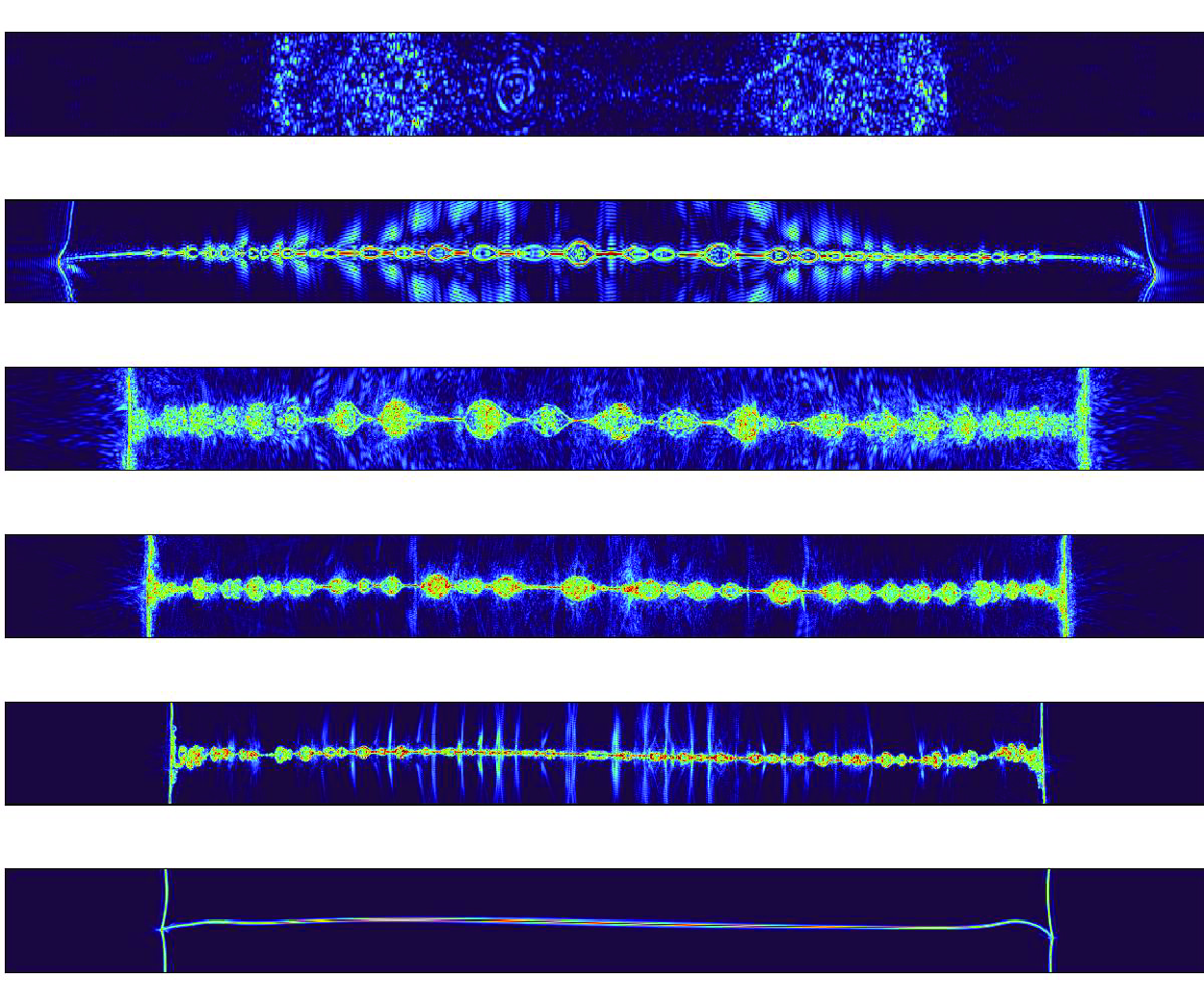
Figure 3. Squared current density for the smallest value of $\eta$ examined (zoomed in on the current layer) for different resolutions $N$ .

The consequences of not using sufficient resolution are severe. In figure 2 we show visualizations of the squared current density (zoomed in on the current layer) obtained from well-resolved runs for different values of $\eta$ . None of these runs displayed visible plasmoids even though values of $S_L=5.4\times 10^5$ are reached. We note that in the bottom two plots, the current layer is visibly not straight. Instabilities have developed that have given a bent shape to the current layer. These structures could be related to Kelvin–Helmholtz instabilities developed due to the strong outflow. However, although instabilities are present, they have not led to plasmoid formation.

In figure 3 we plot the squared current density again for the smallest value of $\eta$ examined for different resolutions $N$ . From these runs, only the last one for $N=32\,768$ is well-resolved based on the dissipation spectrum as discussed before. It is striking that all under-resolved runs displayed plasmoids. In fact, the worse the under-resolving is, the larger the plasmoids appear. This phenomenon is also present at smaller values of $\eta$ examined: when the flow is not well-resolved plasmoids are present. Table 1 shows the parameters used for all runs (not just those shown in figures 2 and 3) indicating the value of resolution $N$ required for each value of $\eta$ so that the simulation is well-resolved. All resolutions smaller than the marked value displayed plasmoids. Similar features due to under-resolving have also been observed in Burger’s and Navier–Stokes turbulence where they have been studied extensively (Ray et al. 2011; Murugan & Ray 2023).

Further insight can be gained by looking at the energy spectra. Figure 4(a) shows the current density spectra for the runs corresponding to figure 2, while the figure 4(b) shows the spectra for the runs corresponding to figure 3. In figure 4(a) all runs are marginally well-resolved. As the resolution is increased and $\eta$ is decreased, $E_J(k)$ progresses to larger wavenumbers forming a $k^0$ power-law range that reflects the approximate discontinuity of the magnetic field in the current sheet. This power-law range is followed by an increase that could be attributed to either a bottleneck (Falkovich 1994; Donzis & Sreenivasan 2010; Agrawal et al. 2020) or a transition to 2-D-MHD turbulence as a result of the instabilities that have developed with $E(k)\propto k^{-5/3}$ . At larger wavenumbers, the spectrum shows a steep exponential decrease. Finally, at the highest wavenumbers near $k_{\it max }$ there is a sharp increase. This is a numerical artefact due to the sharp spectral truncation that leads to a partial thermalisation of high wavenumbers (Cichowlas et al. 2005; Alexakis & Brachet 2020). This peak is observed in all moderately resolved pseudospectral simulations. The Fourier modes at these high wavenumbers have random phases and act as random noise. If not controlled, they can provide a seed for numerical instabilities. Further increasing the resolution for a given value of $\eta$ has little effect as is demonstrated in the inset of the figure 4(b) where the well-resolved run for $N=1024$ (plotted in figure 4(a) is repeated at larger resolutions $N=2048$ and $N=4096$ . No additional features were observed in any of the runs when the resolution was increased further, indicating that the simulations correctly capture the solution of (2.2).

The behaviour described above changes when the resolution is small. In figure 4(b), where only the simulation with the largest $N$ is well-resolved, clear under-resolving features can be testified. As the resolution is decreased the amount of energy at the largest wavenumbers increases changing the shape of the spectrum. It is worth noting that the integral of $E_J(k)$ is proportional to the Ohmic dissipation and even at the second to largest resolution $N=16\,384$ the Ohmic dissipation due to the wavenumbers at $k_{\it max }$ is comparable to the dissipation due to the peak of $E_J(k)$ around $k=500$ . It is thus not surprising that not being well-resolved leads to erroneous estimates of the reconnection rate and appearance of plasmoids.

Figure 4. Squared current density spectra corresponding to the runs shown in figures 2 (a) and 3 (b).

Figure 5. (a) Reconnection rate as a function of $S_L$ for all runs well-resolved (filled symbols) and under-resolved (open symbols). (b) Width of the reconnection layer normalized by the grid size as function of $S_L$ .

This is clearly demonstrated in figure 5 where the reconnection rate $RR$ is plotted as a function of $S_L$ for all our simulations. Different colours represent different resolutions used. Filled symbols correspond to well-resolved runs while open symbols correspond to under-resolved runs. All well-resolved runs display the Sweet–Parker scaling $RR\propto S_L^{-1/2}$ even up to $S_L= 5 \times 10^{5}$ that corresponds to the run at $N=32\,768$ . When the runs are under-resolved, however, deviations from this scaling appear, leading to a $S_L-$ independent scaling. This, however, is a numerical artefact. The reason can be linked to the thickness of the current sheet. In figure 5(b), we plot the thickness of the current layer defined as $\delta \equiv B_{\it max }/j_{max}$ normalized by the grid size $\triangle x=2\pi /N$ for all runs as well. Well-resolved runs follow again the Sweet–Parker prediction $\delta \propto S_L^{-1/2}$ but this scaling obviously ceases to be true when the width of the current sheet is comparable to the grid size.

4. Conclusions

The present work investigated the formation of a magnetic reconnection layer in the Orszag–Tang configuration paying particular attention to the effects of numerical resolution. The main result is that in the present set-up no plasmoid instability was seen for the examined range of Lundquist numbers for well-resolved runs, while on the contrary under-resolved runs displayed plasmoids whose size and population depended on the level of under-resolution. The reasons why insufficient resolution can lead to the formation of plasmoids are obvious: reconnection is a topological change of field lines that can only be broken by some microscale process. Under-resolving can be such a process although not a physical one. It is hard to imagine that continuity of field lines can be preserved when the finiteness of the grid size is apparent. Thus in under-resolved cases the flow can reach states that otherwise would be absent. The present work therefore rings a bell on the artificial effects finite grid resolution can have on the evolution of magnetic and velocity fields in numerical simulations, when not properly resolved. Our results add to those of Wan et al. (2009, 2010, 2013) and Ng & Ragunathan (2011) by focusing on a single reconnection layer, allowing more precise statements to be made.

The results bring out the question of why the plasmoid instability is still not present even though such high Lundquist numbers are reached when the analytical results of idealized reconnection layers (Loureiro et al. 2007; Samtaney et al. 2009; Loureiro et al. 2013a ) predict instabilities at lower $S_{_L}$ than those achieved here. There could be various reasons why this apparent mismatch is present. First, we need to note that the Orszag–Tang configuration used here is different in many respects from the idealized models used in linear theory works. The flow here is time evolving and of finite extent and with an order one initial velocity amplitude. All these factors could play a role in delaying the onset of the plasmoid instability. In Loureiro et al. (2007), the role of the finite extent was estimated by assuming that the predicted growth rate has to be such that a plasmoid has time to grow before it is ejected from the layer. The same argument can also be made for the finite time duration of the layer examined here. This kind of arguments, however, although very reasonable assume that the perturbations existing in the layer are not too small so that the exponential increase of the instability has the time to bring them to the nonlinear regime. Clearly if the perturbation amplitude is several times smaller than $A e^{-\gamma T}$ (where $\gamma$ is the perturbation growth rate, $T$ the typical time duration of the reconnection layer and $A$ the amplitude that makes the perturbation nonlinear), no plasmoids would be formed. In the present set-up, the initial perturbations are large enough to be visible in figure 1. These perturbations, however, decrease at the early stages of the evolution. Thus, even if the linear instability threshold is crossed at later times, they never have the time to grow back up. Perhaps if larger perturbations were introduced in the initial conditions, plasmoid would appear in the well -resolved runs. In some studies (Ng & Ragunathan 2011), additional noise is introduced in the flow at the time the current layer is formed that triggers the plasmoid instability. Such additional noise could model some other mechanisms (as the microscale process mentioned in the introduction) that take place at small scales and lead to a change of field line topology. Under-resolvement could also play artificially that role. Such microscale process can provide the seed that could lead to the formation of plasmoids. Such practice, however, deviates from the solutions of the 2-D-MHD equations and it is not followed here. Another possibility would be to study a different velocity–magnetic field configuration that could possibly lead to more tractable values of the Lundquist number where the plasmoid instability could be observed. Whether plasmoids are present or absent under general configurations is an important issue with major implications for astrophysical plasmas. We hope that this work will motivate further studies in this direction.

Whatever may be the reasons for which plasmoids do not appear in the present set-up, it remains indisputable that if the resolution is small they do artificially appear. This is a result that can be tested even at small resolutions as indicated in table 1. Thus, the numerical error due to the finite computational grid can lead to structure formation that is not present in the solution of the partial differential equation and has possibly led to erroneous conclusions. This emphasizes the need for convergence studies in numerical simulations and indicates that some of the conclusions for magnetic reconnection due to plasmoids in 2-D-MHD based on numerical simulations need to be re-evaluated.