Large-eddy simulations of turbulent flow in a channel with streamwise periodic constrictions

Abstract

We perform large-eddy simulations of turbulent flow in a channel constricted by streamwise periodically distributed hill-shaped protrusions. Two Reynolds number cases, i.e. $Re_h=10\,595$ (Fröhlich et al., J. Fluid Mech., vol. 526, 2005, pp. 19–66) and $Re_h=33\,000$ (Kähler et al., J. Fluid Mech., vol. 796, 2016, pp. 257–284), are repeated and utilized to verify and validate our numerical results, including the pressure and skin friction coefficients on bottom and top walls of the channel, mean velocity profiles and Reynolds stresses. All comparisons show reasonable agreement, providing a measure of validity that enables us to further probe simulation results at higher Reynolds number ($Re_h=10^5$) into aspects of flow physics that are not available from experiments. Effects of variation of Reynolds number are studied, with emphasis on the mean skin friction coefficients, separation bubble size and pressure fluctuations that are related to separation and reattachment. In addition, the main large-scale features of the separation behind the hill, including the scaling of the mean velocity profiles, are discussed. Furthermore, the instantaneous near-wall flow field is analysed in terms of skin friction portraits, and we confirm the existence of the local very small separation bubble on the hill crest as observed in experimental and numerical investigations. The flow field at the top wall, which is generally not given sufficient attention, is evaluated with the empirical friction law and universal logarithmic law as in planar channel flows. It is found that these empirical laws compare well with the large-eddy simulation results, although the hill constrictions behave as a perturbation source and the developed shear layer has some effects on the flow field near the top wall.

1. Introduction

Flows over curved surfaces, involving unsteady separation and reattachment in space and time, occur in numerous engineering applications, such as engine nacelles, curved ducts, bluff bodies and so on. For such complex flows, it is quite challenging to accurately predict the separation and reattachment behaviour at affordable computational cost (Larsson et al. 2016; Bose & Park 2018). In particular, the separation location fluctuates spatially and temporally, and strongly affects the downstream flow structures including the subsequent reattachment process.

Flow over a periodic arrangement of smoothly contoured two-dimensional hills (ERCOFTAC test case 81) has in recent years become one of the most widely used test cases to investigate the physics of turbulent separated flows over curved surfaces, as well for validation of computational fluid dynamics codes and turbulence models (Rodi, Bonnin & Buchal 1995). The configuration of periodic channel flow was originally proposed by Almeida, Durao & Heitor (1993), and then modified by Mellen, Fröhlich & Rodi (2000) to be more suitable for numerical simulations. The history of this case is found in the review paper by Breuer et al. (2009). The periodic hills geometry has been investigated both numerically and experimentally over a wide range of Reynolds numbers. Mellen et al. (2000) investigated the periodic hill flow at $Re_h = 7100$ (based on hill height $h$ and bulk mean velocity through the hill crest $U_b$) using wall-modelled and wall-resolved large-eddy simulations (WMLES and WRLES), and the impact of different subgrid-scale (SGS) models and grid qualities was assessed. A similar investigation was carried out by Temmerman et al. (2003) at $Re_h = 10\,595$ using WMLES, which combined different SGS models and wall-law functions. It was demonstrated that the flow features are surprisingly more sensitive to the wall model than the SGS model, and the classical wall models developed for attached flows are not satisfactory for this flow. Fröhlich et al. (2005) performed highly resolved (only the bottom wall) incompressible LES at $Re_h = 10\,595$ using two different second-order finite-volume discretizations with two different SGS models, i.e. the dynamic Smagorinsky model (Germano et al. 1991) and the ‘wall-adapted local eddy-viscosity’ model (Ducros, Nicoud & Poinsot 1998). A detailed analysis of structural characteristics of this flow configuration has revealed a number of interesting features. Breuer et al. (2009) presented a comprehensive review of direct numerical simulations (DNS) and WRLES performed to date, comparing experimental data with numerical results using DNS up to $Re_h = 5600$ and WRLES up to $Re_h = 10\,595$. Rapp & Manhart (2011) experimentally investigated this flow at four Reynolds numbers $(5600 \leqslant Re_h \leqslant 37\,000)$ with two-dimensional particle image velocimetry and one-dimensional laser Doppler anemometry measurements. The streamwise periodicity of the flow and sidewall effects were evaluated, together with investigations of Reynolds number effects. Kähler, Scharnowski & Cierpka (2016) repeated the experiment $(Re_h=8000,33\,000)$ with high-resolution particle image velocimetry and particle tracking velocimetry techniques. This high-resolution measurement makes possible a precise analysis of the near-wall flow features. Recently, Krank, Kronbichler & Wall (2018) presented DNS at $Re_h=5600$ and $10\,595$ using spectral incompressible discontinuous Galerkin schemes. Although many DNS and LES have been performed for $Re_h \leqslant 10\,595$, there has been somewhat limited research for larger Reynolds numbers due to extremely high-resolution requirements in the near-wall region. To the best of our knowledge, only two hybrid Reynolds-averaged Navier–Stokes (RANS)/LES have been performed at $Re_h=37\,000$ (Chaouat & Schiestel 2013; Mokhtarpoor, Heinz & Stoellinger 2016). For wall-bounded turbulent flows, a tenable solution for investigating higher-Reynolds-number cases is to employ the wall modelling approach since the mesh resolution requirement of WMLES scales linearly with increasing $Re$ (Choi & Moin 2012).

In the past four decades, several wall models have been proposed for canonical flows in simple geometries (Schumann 1975; Grötzbach 1987; Piomelli et al. 1989; Marusic, Kunkel & Porté-Agel 2001; Piomelli & Balaras 2002). The reader is referred to the review paper by Bose & Park (2018) for recent developments of wall model techniques. However, there are a couple of primary challenges when it comes to flow over curved surfaces. First, most wall models follow the equilibrium stress assumption and imply a logarithmic-law profile in the near-wall region, which breaks down when turbulent boundary layers are subjected to strong adverse pressure gradients leading to separation, extra strain due to curvature, etc. (Diurno 2001; Bose & Park 2018). Meanwhile, some enhanced wall-function models, which take into account the streamwise pressure gradient, have been developed to simulate flow over periodic hills (Breuer, Kniazev & Abel 2007; Manhart, Peller & Brun 2008; Duprat et al. 2011), but the free parameters in these models restrict their application in general. Second, most wall modelling strategies including detached eddy simulations (DES) fall into the hybrid RANS/LES methodology in complex geometries, which solves the RANS equations in the inner layer and provides wall shear stress boundary conditions for the outer LES region (Cabot & Moin 1999; Piomelli & Balaras 2002; Kawai & Asada 2013; Park & Moin 2016). This hybrid method is not only sensitive to the choice of the RANS model and its associated model coefficients, but also causes the so-called ‘scale disparity’ problem on the nominal interfaces between the RANS and LES regions (Germano 2004; Piomelli 2008). Alternatively, Chung & Pullin (2009) proposed the virtual wall model, which dynamically couples the outer resolved region with the inner wall region, and offers a slip velocity boundary condition for the filtered velocity field on the ‘virtual’ wall. This wall model has been successfully deployed in canonical flows without separation (Inoue & Pullin 2011; Saito, Pullin & Inoue 2012), and then extended by Cheng, Pullin & Samtaney (2015) to simulate flat-plate turbulent boundary layer flows with separation and reattachment. Recently, this virtual wall model was extended to generalized curvilinear coordinates by Gao et al. (2019) and utilized in WMLES for flow past airfoils. The same framework is adopted and tested in the present simulations.

Turbulent boundary layer flow over a curved surface, involving separation and reattachment, generates larger pressure fluctuations than that in the equilibrium boundary layer. Wall-pressure fluctuations play a key role in a variety of engineering applications, such as flow-induced panel flutter and structural vibration, aircraft cabin noise and hydroacoustics of underwater vehicles (Blake 1970). Many investigations of wall-pressure fluctuations beneath a turbulent boundary layer have been performed in the past several decades, including zero pressure gradient turbulent boundary layer (Bradshaw 1967; Willmarth 1975; Farabee & Casarella 1991); flat-plate turbulent boundary layers with adverse pressure gradient (Mabey 1972; Simpson, Ghodbane & McGrath 1987; Na & Moin 1998a,b; Abe 2017); and turbulent flows over a backward- or forward-facing step (Farabee & Casarella 1986; Ji & Wang 2012; Awasthi et al. 2014; Doolan & Moreau 2016). Presently, for turbulent flow in a channel with streamwise periodic constrictions, we analyse the pressure fluctuations by relating these to the mean pressure in the separation bubble and the development of the mixing layer.

In the present investigation, we emphasize three main objectives. First, the extended virtual wall model developed by Gao et al. (2019) is applied in a periodic channel flow (both bottom and top walls). All the WMLES results are validated with experimental data wherever available. Some WRLES results are also utilized for verifications, especially the pressure and skin friction coefficients which are not reported in the experiments but are important in separation and reattachment. Based on these verifications and validations, the effects of Reynolds number on the skin friction coefficient, separation bubble size and pressure fluctuations are analysed. Second, the details of unsteady separation in this flow have not been reported in the past. Recent work by Cheng, Pullin & Samtaney (2017, 2018) in WRLES of flow past a smooth and grooved cylinder at subcritical and supercritical Reynolds numbers emphasized the role of unsteady separation and the dynamics of separation bubbles in the phenomenon of the drag crisis. They attributed the drag crisis, mainly due to a large change in form drag, to the topology change induced by the movement of the location of curvature-controlled large-scale separation. In the present study, the periodic hill channel may be considered as a combination of flat and curved surfaces, and this geometric complexity would result in rich flow physics associated with separation and reattachment. The last main objective comes from the fact that almost all of the previous investigations paid little attention to the flat top wall of the channel. The empirical friction law and universal logarithmic law, which are well captured in plane channel flows, are also evaluated from the top wall of the channel.

The paper is organized as follows. In § 2, we describe the physical set-up, followed by a discussion of the governing equations, and briefly discuss wall and SGS models employed (details are relegated to appendices). In § 3, the WMLES results are validated and verified with experimental and WRLES results. After that, in §§ 4 and 5, we provide new insights based on LES results up to $Re_h=10^5$. The flow near the bottom wall is analysed in § 4, emphasizing on the separation/reattachment behaviour. Here we investigate scaling relations for the skin friction coefficient and velocity profiles in separation zones. Instantaneous skin friction lines at three $Re_h$ are compared, with focus on the existence of a small separation bubble near the top of the hill. Further in § 5, the flow at the top wall is characterized using the empirical friction law and universal logarithmic law which are proposed for planar channel flow. Finally, the conclusions are drawn in § 6.

2. Physical and numerical set-up, equations and models

In this section, the flow configuration is described, and following that we present the essential set of equations including the boundary conditions at the virtual wall required to perform WMLES in a wall-bounded domain. The detailed derivations for the wall model in the generalized curvilinear coordinates were given by Gao et al. (2019). We include the details of the wall model, the SGS model and the numerical methods in appendices for the sake of completeness.

2.1. Flow configuration

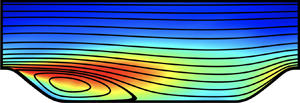
We perform LES of turbulent flow past periodically constructed hills on the bottom wall in a channel with a flat wall on the top. The physical geometry and simulation domain are illustrated in figure 1. The shape of the hill is defined in the form of a polynomial, taken from the experimental study by Almeida et al. (1993). This is also a standard test case for an ERCOFTAC/IAHR workshop, and has been widely used to validate various numerical schemes and physical models. It should be noted that geometry G1 (figure 1a) was adopted in WRLES by Fröhlich et al. (2005) for $Re_h=10\,595$ and geometry G2 (figure 1b) was the region of focus in the experimental investigations of Kähler et al. (2016). These two geometries are essentially identical since the hills are constructed periodically in the $x$ direction. For the sake of simplicity of verifications and validations, G1 is adopted in the case of $Re_h=10\,595$, while G2 is used for the cases of $Re_h=33\,000$ and $Re_h=10^5$.

Figure 1. Sketch of the hill geometry adopted in the present paper. (a) Geometry G1: simulation geometry adopted in the present WMLES and WRLES of Fröhlich et al. (2005) for $Re_h=10\,595$; (b) geometry G2: simulation geometry adopted in the present WMLES and WRLES and experimental domain of Kähler et al. (2016) for $Re_h=33\,000$.

2.2. Governing equations

To compute the flow in this set-up, assuming constant (unity) density, we solve the filtered incompressible Navier–Stokes equations on a body-fitted curvilinear grid. In generalized curvilinear coordinates, the equations of motion are

(2.1)\begin{gather} \frac{\partial U^m}{\partial \xi^m} =0, \end{gather}

(2.2)\begin{gather}\frac{\partial \left(\sqrt g u_i\right)}{\partial t} + \frac{\partial F_i^m}{\partial \xi^m} =0, \end{gather}

where $(\xi ^1,\xi ^2,\xi ^3)=(\xi ,\eta ,\zeta )$ denote the generalized curvilinear coordinates; $U^m$ (the volume flux normal to the surface of constant $\xi ^m$) and $F_i^m$ are given by

(2.3)\begin{gather} \left.\begin{array}{c} \displaystyle U^m = {\sqrt g} \frac{\partial \xi^m}{\partial x_j} u_j, \\ \displaystyle F_i^m = U^m u_i + {\sqrt g} \frac{\partial \xi^m}{\partial x_i} p - \nu {G}^{mn} \frac{\partial u_i}{\partial \xi ^n}, \\ \displaystyle \sqrt g = J ^{-1} = \det \left[\frac{\partial x_i}{\partial \xi^j} \right ],\quad {G}^{mn} = \sqrt g \frac{\partial \xi^m}{\partial x_r}\frac{\partial \xi^n}{\partial x_r}, \end{array}\right\} \end{gather}

where $(x_1,x_2,x_3)=(x,y,z)$ are the Cartesian coordinates with corresponding velocity components $(u_1,u_2,u_3)=(u,v,w)$, $p$ is the pressure, $\nu$ is the kinematic viscosity, $J^{-1}$ is the Jacobian of the transformation and $ {G}^{mn}$ is the mesh skewness tensor. It should be noted that the $\zeta$ direction is congruent with the $z$ direction since the spanwise geometry is uniform in the present research. Applying a nominal filter to the incompressible Navier–Stokes equations, the filtered LES equations are written below in terms of the resolved velocity field:

(2.4)\begin{gather} \tilde {U}^m = {\sqrt g} \frac{\partial \xi^m}{\partial x_j} \tilde{u}_j, \end{gather}

(2.5)\begin{gather}\tilde{F}_i^m = \tilde{U}^m \tilde{u}_i + {\sqrt g} \frac{\partial \xi^m}{\partial x_i} \tilde{p} - \nu {G}^{mn} \frac{\partial \tilde{u}_i}{\partial \xi ^ n} + {\sqrt g}\frac{{\partial {\xi ^m}}}{{\partial {x_j}}}{{T}_{ij}}, \end{gather}

where tildes denote filtered quantities and $ {T}_{ij} = \widetilde {u_iu_j} - \tilde u_i \tilde u_j$ is the SGS stress tensor. The stretched spiral vortex model is adopted to compute $ {T}_{ij}$, details of which are in appendix A.

2.3. Boundary conditions

For the simulations, periodic boundary conditions are prescribed in the spanwise and streamwise directions. The spanwise extent ($L_z$) is of importance in order to obtain reliable and physically reasonable results. To ensure this criterion, the two-point correlations in the spanwise direction have to decay to sufficiently small values in the half-width of the domain size chosen. Based on the investigations by Mellen et al. (2000), a spanwise extension of the computational domain of $L_z=4.5h$ is used in all computations presented. This spanwise domain extent was also used in the investigation by Fröhlich et al. (2005) and many other DNS/LES studies (Breuer et al. 2009; Krank et al. 2018). It represents a well-balanced compromise between spanwise extent and spanwise resolution.

For boundary conditions on the solid walls (both bottom and top walls), the no-slip boundary condition is specified at the actual wall in WRLES, and a Dirichlet boundary condition for the velocity, derived from the wall model, is specified at the virtual wall in WMLES. Similar to the turbulent plane channel flow case, the non-periodic behaviour of the pressure field is accounted for by inclusion of a mean pressure gradient as a source term in the streamwise momentum equation. Two alternatives are possible: either the pressure gradient is fixed which results in a fluctuating mass flux or the mass flux is held constant which requires adjustment of the mean pressure gradient in time. Since a fixed Reynolds number can only be guaranteed by a fixed mass flux, the second option is chosen using the method proposed by Benocci & Pinelli (1990).

2.4. Wall model

The virtual wall model in generalized curvilinear coordinates developed by Gao et al. (2019), coupled with the stretched vortex SGS model, has been strongly verified and validated in various airfoil flows. We briefly describe the essential idea of the wall model with details relegated to appendix B. It should be noted that, consistent with other approaches involving body-fitted mesh computations, the computational mesh is constrained to be locally orthogonal to the solid walls for wall-normal averaging, and the wall-normal coordinate is denoted as $y_n$. As shown in figure 2, the distance $h'$ is typically chosen as the distance of the first grid point from the solid wall and $h_0$ is the height of the virtual wall that is further discussed below.

Figure 2. Sketch of the near-wall velocity components. The dashed line above the solid wall denotes the virtual wall, and the blue point denotes the centre of the first grid cell off the solid wall.

We define the magnitude of the resultant velocity $\tilde q$ and velocity angle $\theta$ on the wall-parallel plane as

(2.6a,b)\begin{equation} \tilde{q} = \sqrt{\tilde{u}_s^2 + \tilde{w}^2},\quad \theta = \arccos\left( \tilde u_s/ \tilde q \right), \end{equation}

where $\tilde {u}_s$ is the streamwise velocity parallel to the solid wall (as shown in figure 2), given by

(2.7)\begin{equation} \tilde{u}_s = \tilde{u} \cos \theta_w + \tilde{v} \sin \theta_w, \end{equation}

where $\theta _w$ denotes the local angle between the solid wall and the $x$ coordinate.

The wall-normal gradient of $\tilde q$, i.e. $\eta _0 (\xi , \zeta , t)$, and the associated friction velocity $u_\tau$ are defined as

(2.8a,b)\begin{equation} \eta_0 \equiv \left. \frac{\partial \tilde q}{\partial y_n} \right |_w,\quad u_\tau = \sqrt{\nu \eta_0}. \end{equation}

Based on the near-wall filtering and wall-normal averaging approach, the following ordinary differential equation (ODE) for $\eta _0$ can then be derived (see appendix B for details):

(2.9)\begin{equation} \frac{\partial \eta_0}{\partial t} = C_1 \eta_0 - C_2 \eta_0^2, \end{equation}

where

(2.10a,b)\begin{equation} C_1 = \frac{2}{\tilde q|_{h'}} \left( F_\xi + F_\zeta +M+ \left.\frac{ \nu {G}^{22}}{\sqrt g {h'}} \frac{\partial \tilde q}{\partial y_n} \right|_{h'} \right),\quad C_2 = \frac{2 \nu {G}^{22}}{\sqrt g {h'} \tilde q|_{h'}}. \end{equation}

Detailed expressions for $F_\xi$, $F_\zeta$ and $M$ are given by (B 10), (B 12) and (B 14), respectively; an approximate analytical solution to (2.9) is given in appendix B.

Once $\eta _0(\xi ,\zeta ,t)$ is known, the velocity angle $\theta (\xi , z, t)$ is estimated as $\arccos (\tilde u_s|_{h'}/\tilde q|_{h'})$ from the first grid cell of the resolved LES field, an approximation justified based on the work of Cheng et al. (2015) (turbulent boundary layer flow with separation and reattachment) and Gao et al. (2019) (separated flow past airfoils). The local wall shear stress components may then be computed as

(2.11a,b)\begin{equation} \tau_{w,s} = \mu \eta_0 \cos \theta,\quad \tau_{w,z} = \mu \eta_0 \sin \theta. \end{equation}

Here $\mu =\rho \nu$ is the dynamic viscosity and ${\boldsymbol {\tau }}_w \equiv (\tau _{w,s}, \tau _{w,z})$ is the LES representation of the surface stress vector. Above, we make the approximation that the velocity angle $\theta$ is constant within the first grid cell, $0 \leqslant y_n \leqslant h$. Cheng et al. (2015) proposed an algebraic model for $\theta$ in turbulent boundary layer simulations and concluded that there is little difference between the constant velocity angle model and the algebraic model. In the present paper, the constant velocity angle model is adopted for simplicity.

Finally, we present a slip velocity $\tilde q|_{h_0}$ on the virtual wall as

(2.12)\begin{equation} \left. \tilde q \right|_{h_0} =\begin{cases} \begin{cases} \quad u_\tau\left( \dfrac{1}{\mathscr{K}_1} \log\left( \dfrac{h_0^+}{h_\nu^+} \right) + h_\nu^+\right) , & h_0^+ > h_\nu^+, \\ \quad u_\tau h_0^+, & h_0^+ < h_\nu^+, \end{cases}& \tau_{w,s} > 0, \\\\ \quad\quad u_\tau\,h_0^+, & \tau_{w,s} \leqslant 0, \end{cases} \end{equation}

where $h_0^+=u_{\tau } h_0/\nu$ and $h^+_\nu$ is the intercept between the linear and logarithmic components in the law of the wall. Experimental research shows that the outer edge of the viscous sublayer is located at $h^+_\nu \approx 11$, which is approximately equivalent to the offset ($=5.0$) in the classical logarithmic law. This empirical value is adopted by Chung & Pullin (2009) and Inoue & Pullin (2011), and also by Cheng et al. (2015) and Gao et al. (2019) in modelling the boundary layer flows with separation and reattachment. In the present case, $h^+_\nu = 11$ is used as an empirical parameter in the wall model. Both $h_0^+$ and $h^+_\nu$ are fixed in all the simulations presented, the same values being used in our previous work, and hence these parameters may not be considered as ‘tunable’ parameters. In the attached region ($\tau _{w,s}>0$), the linear–logarithmic relation is essentially the same as that of Chung & Pullin (2009), which is derived from the stretched-vortex SGS model (see appendix A) and the Kármán-like constant $\mathscr {K}_1$ is dynamically computed. In the separated region ($\tau _{w,s} \leqslant 0$), the log-like relation is no longer valid and Cheng et al. (2015) proposed a linear relationship which appears to work reasonably well in regions of flow separation. Here, we follow the linear law of Cheng et al. (2015).

Based on the above formulation, the wall model can be summarized as follows. In the near-wall region, (2.9) is solved for $\eta _0$, in which the coefficients on the right-hand side are approximated with the resolved LES field at the first grid cell, i.e. $h'=h_0+{\rm \Delta} y_n/2$ (the choice of $h_0$ is given in appendix B). Equation (2.12) is then used to compute the resultant velocity $\tilde q|_{h_0}$ on the virtual wall with the streamwise and spanwise velocity components given by

(2.13a,b)\begin{equation} \tilde u_s|_{h_0} = \tilde q|_{h_0} \cos \theta,\quad \tilde w|_{h_0} = \tilde q|_{h_0} \sin \theta. \end{equation}

The contribution of the wall-normal velocity component $\tilde u_n|_{h_0}$ to $\tilde u$ and $\tilde v$ is assumed to be small comparing with $\tilde u_s|_{h_0}$, and we use $\tilde u_n|_{h_0}=0$. Finally, the slip velocity boundary condition on the virtual wall $y_n=h_0$ is

(2.14a,b)\begin{equation} \tilde u|_{h_0} = \tilde q|_{h_0} \cos \theta \cos \theta_w, \quad \tilde v|_{h_0} = \tilde q|_{h_0} \cos \theta \sin \theta_w, \end{equation}

with the spanwise velocity component $\tilde w|_{h_0}$ given by (2.13b).

2.5. Summary of numerical cases

Three cases, as summarized in table 1, are considered. The energy-conservative fourth-order finite-difference scheme is used for spatial discretizations, and the discretized governing equations are solved using a semi-implicit fractional step method (see appendixC for details). For $Re_h=10\,595$, only WMLES is performed and compared with both WRLES from Fröhlich et al. (2005) and experimental data from Rapp & Manhart (2011). To check the effects of mesh resolution on the WMLES, a mesh convergence study of this case is presented in appendix D. For $Re_h=33\,000$, neither the pressure nor skin friction coefficients were measured in the experimental investigation of Kähler et al. (2016); thus we perform both WRLES and WMLES. Accurate predictions of the separation and reattachment depend on the skin friction coefficient, which is also challenging in terms of wall modelling especially for flow over complex geometries. The WRLES results are utilized to verify the WMLES results for some quantities that were not reported in the experiment for $Re_h=33\,000$. Furthermore, the WRLES (R2) case not only resolves the flow at the lower wall but also resolves the upper wall by a DNS-like representation. We briefly remark that the computational expense of WMLES is approximately 12 times that of WMLES per time interval with the same CPU cores. The grid spacings in the wall-normal direction (i.e. $\eta$ direction) on both the bottom and top walls are illustrated in figure 3, and the mesh size ratios are also given in table 1. Note that we employ a higher resolution in the spanwise direction than the streamwise direction for case M1. For cases M2 and M3 the resolution in terms of (${\rm \Delta} \xi ^+/ {\rm \Delta} \eta ^+_b$, ${\rm \Delta} z^+/ {\rm \Delta} \eta ^+_b$) is (5.1, 7.0) for M2 and (4.1, 7.0) for M3, respectively. We believe that the disparity in resolution between the spanwise and streamwise directions is not severe within the context of WMLES.

Figure 3. Dimensionless wall-normal grid spacings in wall units ${\rm \Delta} \eta ^+_{(b,t)}$: (a) bottom wall and (b) top wall. , WMLES for $Re_h=10\,595$; , WRLES for $Re_h=33\,000$; , WMLES for $Re_h=33\,000$; , WMLES for $Re_h=10^5$. Note that the right-hand $y$ axis is for WRLES.

Table 1. Summary of the performed numerical cases. The ‘$+$’ superscript indicates the expression of the mesh quantities using wall units and the subscripts ‘$b$’ and ‘$t$’ denote the bottom and top walls, respectively. Time $t_r=9h/U_b$ is the typical flow-through time and $t_{a}$ is the total simulation time.

3. Numerical results for statistically averaged quantities

In this section, we present several time- and spanwise-averaged quantities that are used to verify and validate the present WMLES/WRLES code: these are the skin friction coefficient, $C_f$; the pressure coefficient, $C_p$; the normalized velocity profiles in $x$ and $y$ directions, $\bar u/U_b$ and $\bar v/U_b$; and the normalized Reynolds stresses profiles, $\overline {u^{\prime }u^{\prime }}/U_b^2$, $\overline {v^{\prime }v^{\prime }}/U_b^2$ and $\overline {u^{\prime }v^{\prime }}/U_b^2$. The Reynolds stress containing SGS corrections to the resolved flow is calculated as $\overline {u'_iu_j'} = \overline {\tilde {u}'_i\tilde {u}_j'} + \overline{{T}}_{ij}$ (Inoue & Pullin 2011). The skin friction coefficient and pressure coefficient are computed as

(3.1a,b)\begin{equation} C_f = \frac{\bar{\tau}_{w,s}}{0.5\rho U_b^2},\quad C_p= \frac{\bar{p}-p_{r}}{0.5\rho U_b^2}, \end{equation}

where $\bar {\tau }_{w,s}$ is the local streamwise (parallel to the actual wall) mean wall shear stress, $\bar {p}$ is the local pressure and $p_{r}$ is a reference wall pressure taken at the centre of the hill crest. In WMLES, $\bar {\tau }_{w,s}$ is computed from the wall model; in WRLES, the third-order accuracy one-sided velocity-derivative method (Cheng et al. 2017) is used for the wall-normal differentiation. It should be noted that all the flow configurations are rescaled to geometryG1 (see figure 1a) for simplicity of investigation, and this compatible coordinate system will be used in the later sections if not mentioned specifically.

3.1. Reynolds number $Re_h=10\,595$

The skin friction coefficient $C_f$ and pressure coefficient $C_p$ for $Re_h=10\,595$ on both the bottom and top walls are shown in figure 4. We compare our results with the highly resolved LES results from Fröhlich et al. (2005) for verification (note that Fröhlich etal. (2005) did not report $C_f$ at the top wall). The present WMLES shows good agreement with the reference LES data, although slightly smaller $C_f$ on the leeward side of the hill within the separation zone, i.e. $x/h \approx 1.0$–$2.0$. The $C_f$ plot shows the primary separation point at approximately $x/h=0.22$, with reattachment at $x/h=4.59$. This compares well with the experimental results of Rapp & Manhart (2011), who reported the reattachment point at $x/h=4.21$. The predicted values also compare well with the WRLES (Fröhlich et al. 2005) values of $x/h=0.20$ and $x/h=4.56$ (see figure 4b), respectively, for the separation and reattachment points. Two very small recirculation regions, one on the hill top, $x/h \approx 0$, and the other in the post-reattachment zone on the windward side of hill, $x/h \approx 7.0\text {--}7.4$, for $Re_h > 200$ are reported by Breuer et al. (2009), and also confirmed for $Re_h =10\,595$ by WRLES (Mellen et al. 2000; Fröhlich et al. 2005) and DNS (Diosady & Murman 2014; Krank et al. 2018). However, the experimental results at $Re_h=8000$ and $33\,000$ from Kähler et al. (2016) do not confirm the existence of the local separation bubble in these regions, and this was attributed to an insufficient duration of time for averaging. These very small separation regions are also absent in the present WMLES, and are further discussed in § 4.5.

Figure 4. (a) Pressure coefficient $C_p$ and (b) skin friction coefficient $C_f$ along the bottom and top walls for $Re_h=10\,595$. The solid and dash-dotted curves are the corresponding results at the bottom and top walls from the present WMLES. In (a), the circles and squares denote $C_p$ on the bottom and top walls from WRLES by Fröhlich et al. (2005); in (b), the circles denote $C_f$ on the bottom wall from WRLES by Fröhlich et al. (2005). The bold grey line denotes the geometry of the channel with streamwise periodic hills. A horizontal dashed line $C_f=0$ in (b) is shown for reference: zero crossing of this line indicates separation/reattachment.

Figure 5 shows the normalized mean velocity profiles ($\bar u/U_b$ and $\bar v/U_b$) in $x$ and $y$ directions along vertical lines at ten different locations, i.e. $x/h=0.05, 0.5,1,2,3,4,5,6,7,8$. Comparisons with experimental data from Rapp & Manhart (2011) show excellent agreement. For profiles in the separation zone, i.e. $x/h=0.5,1,2,3,4$, negative back flow is noted near the bottom wall (see figure 5a), and the peak value of the back-flow velocity occurs at $x/h=2$, close to the centre of the main separation zone. The steep velocity gradient near the top wall is also captured by the present wall model, which is absent in WRLES by Fröhlich et al. (2005) due to low mesh resolution near the top wall in their simulation. Since the total mass flux through the channel was fixed, the poor prediction of $\bar u/U_b$ near the top wall has a certain influence on the overall flow development (Breuer et al. 2009). The peak value of $\bar v/U_b$ is observed at $x/h=8$ (see figure 5b) due to strong acceleration on the windward side of the hill (see also figure 4a for the pressure distributions).

Figure 5. Normalized mean velocity profiles in the $x$ direction (a) and $y$ direction (b) for $Re_h=10\,595$. From left to right, the mean velocity profiles are located at $x/h=0.05,0.5,1,2,3,4,5,6,7,8$. For the sake of clarity these profiles are shifted by $2$ and $0.5$ for $\bar u/U_b$ and $\bar v/U_b$, respectively. $\circ$, Experiment by Rapp & Manhart (2011); , present WMLES.

Figure 6 shows the normalized Reynolds stresses profiles ($\overline {u^{\prime }u^{\prime }}/U_b^2$, $\overline {v^{\prime }v^{\prime }}/U_b^2$ and $\overline {u^{\prime }v^{\prime }}/U_b^2$) at the same locations where profiles of mean velocity were presented above. Both $\overline {v^{\prime }v^{\prime }}/U_b^2$ and $\overline {u^{\prime }v^{\prime }}/U_b^2$ agree quite well with the experimental and WRLES results. However, deviations are visible for $\overline {u^{\prime }u^{\prime }}/U_b^2$ in the range $x/h=4$–$6$. Considering only the post-reattachment region at $x/h=5$, the measured peak values of $\overline {u^{\prime }u^{\prime }}/U_b^2$ are at most $8\,\%$ higher than in the present WMLES. Nevertheless, the locations of the peak values compare well with both experimental and WRLES results. In the separation zone, $x/h=0.5$–$3$, these comparisons are very satisfactory. In the vicinity of the top wall, the steep variations of $\overline {u^{\prime }u^{\prime }}/U_b^2$ are captured by the present WMLES but absent in WRLES of Fröhlich et al. (2005). The maximum $\overline {v^{\prime }v^{\prime }}/U_b^2$ and $\overline {u^{\prime }v^{\prime }}/U_b^2$ occurs in the separation zone, inside the constant $C_p$ region (see figure 4a), in which flow deceleration and acceleration occur alternately.

Figure 6. Normalized Reynolds stress profiles: (a) $\overline {u^{\prime }u^{\prime }}/U_b^2$, (b) $\overline {v^{\prime }v^{\prime }}/U_b^2$ and (c) $-\overline {u^{\prime }v^{\prime }}/U_b^2$ for $Re_h=10\,595$. From left to right, the Reynolds stress profiles are located at $x/h=0.05,0.5,1,2,3,4,5,6,7,8$, shifted by $0.1$ along the abscissa. $\circ$, Experiment by Rapp & Manhart (2011); , present WMLES; , WRLES from Fröhlich et al. (2005).

3.2. Reynolds number $Re_h=33\,000$

The skin friction coefficient $C_f$ and pressure coefficient $C_p$ for $Re_h=33\,000$ on both the bottom and top walls are shown in figure 7. The present WRLES (case R2) is used to verify the performance of the wall model. Similar to that for $Re_h=10\,595$, a nearly constant pressure plateau is observed in the $C_p$ distribution from the separation point to the centre of the separation zone ($x/h \approx 2$). The skin friction coefficient $C_f$ in the present WMLES is slightly smaller than that from WRLES in the separation zone ($x/h \approx 1.5\text {--}2.5$). Overall, the present WMLES results agree well with the WRLES results. The separation and reattachment points from the present WMLES $C_f$ plot occur at approximately $x/h=0.27$ and $x/h=3.94$, respectively. These predictions are comparable to the corresponding values of $x/h=0.27$ and $x/h=3.96$ from the present WRLES (see figure 7b). These also match well with the experimental results of Kähler et al. (2016), who reported the separation point at $x/h=0.34 \pm 0.05$ and the reattachment point at $x/h=3.80\pm 0.05$. Compared with the $Re_h=10\,595$ case, the peak value of $C_f$ in both attached and separated zones decreases, confirming the observations by Breuer et al. (2009). Furthermore, the undulations in $C_f$ at the beginning of the main separation bubble seem to be related to geometry and not much affected by Reynolds number effects. The very small separation zone at the hill top is detected in the region from $x/h=8.932$ to $9.985$ in the present WRLES, but absent in the WMLES, as was also the case for $Re_h=10\,595$. The very small separation bubble at the foot of thewindward side of the hill does not occur in either simulation from an inspection of the $C_f$ plot.

Figure 7. (a) Pressure coefficient $C_p$ and (b) skin friction coefficient $C_f$ along the bottom and top walls for $Re_h=33\,000$. $\circ$, $C_p$ and $C_f$ on the bottom wall from the present WRLES; $\square$, $C_p$ and $C_f$ on the top wall from the present WRLES; , $C_p$ and $C_f$ on the bottom wall from the present WMLES; , $C_p$ and $C_f$ on the top wall from the present WMLES. The bold grey line denotes the geometry of the channel with streamwise periodic hills. A horizontal dashed line $C_f=0$ in (b) is shown for reference: zero crossing of this line indicates separation/reattachment.

Figure 8 shows the normalized mean velocity profiles in $x$ and $y$ directions along vertical lines at $17$ different locations, i.e. $x/h \in [0,9]$, with a constant gap distance of $0.5$. Comparisons with experimental data from Kähler et al. (2016) show good agreement, although the $\bar v/U_b$ profile at $y/h \approx 1.0$ (in the separated shear layer) is slightly smaller than the measured values after the separation point (see figure 8b). Overall, the shape of the mean velocity profiles is similar to that for $Re_h=10\,595$ at the same locations, which may be construed as agreement with the $Re$-independent behaviour suggested by Kähler et al. (2016). For profiles in the separation zone, i.e. $x/h=0.5\text {--}3.5$, a negative back-flow velocity is clearly observed near the bottom wall (see figure 8a), and the peak value of the back-flow velocity occurs at $x/h=2.0$, close to the centre of the main separation zone. The steep velocity gradient near the top wall is also captured by the present wall model (see also figure 8a). The peak value of $\bar v/U_b$ is visible at $x/h=8.5$ (see figure 8b) due to strong acceleration on the windward side of the hill, similar to the case for $Re_h=10\,595$. The magnitude of this extremum is larger than that in the $Re_h=10\,595$ case, and the vertical location is shifted towards the bottom wall. This is in accordance with the trend described by Breuer et al. (2009) and Kähler et al. (2016). The downward flow ($\bar {v}/U_b <0$) enhances the momentum transfer from the upper half of the channel to the separation zone, which is fed by the outer high-momentum fluid, and thus promotes earlier reattachment compared with the $Re_h=10\,595$ case.

Figure 8. Normalized mean velocity profiles in the $x$ direction (a) and $y$ direction (b) for $Re_h=33\,000$. From left to right, the mean velocity profiles are located at $x/h \in [0,9]$ with gap distance of 0.5, shifted by $2$ and $0.5$ for $\bar u/U_b$ and $\bar v/U_b$, respectively. $\circ$, Experiment by Kähler et al. (2016); , present WMLES; , present WRLES.

Figure 9 shows the normalized Reynolds stress profiles at the same monitoring locations. For flow outside the developing shear layer, i.e. $y/h<0.5$ and $y/h>1.5$, both WMLES and WRLES results compare well with the experimental data from Kähler etal. (2016), but WRLES overpredicts the $\overline {u^{\prime }u^{\prime }}/U_b^2$ profiles in the vicinity of the bottom wall, especially in the post-separation zone (see figure 9a). The overshoot of the Reynolds stresses after the hill top ($x/h>0$) is also captured well by the simulations. In the separated shear layer region, both WMLES and WRLES overpredict the three Reynolds stress components, but WRLES matches better with the peak values of these profiles. Bose & Park (2018) argued that the proper resolution of the separated shear layer is critical in WMLES, and Kähler et al. (2016) also reported that the unresolved mixing process in the simulations and insufficient averaging time (time for ensemble averaging in the LES and DNS should be 12–48 times longer) could also affect the flow statistics. The contribution of the SGS stress to the total Reynolds stress is shown in appendix E, and we found that the fraction of the SGS stress is larger for $Re_h=33\,000$ than $Re_h=10\,595$, especially in the separated shear layer. Nevertheless, the reason behind these discrepancies should be explored further. The peak from the experiment displays a narrower distribution than the present LES. The maximum $\overline {u^{\prime }u^{\prime }}/U_b^2$ occurs upstream of the primary separation point, similar to $Re_h=10\,595$, because we expect larger fluctuations in the region where the transition from attached to separated flow states occurs. The maximum $\overline {v^{\prime }v^{\prime }}/U_b^2$ and $\overline {u^{\prime }v^{\prime }}/U_b^2$ is also located in the constant $C_p$ region, similar to the $Re_h=10\,595$ case. These qualitative observations are also in accordance with the experimental research of Kähler et al. (2016).

Figure 9. Normalized Reynolds stress profiles: (a) $\overline {u^{\prime }u^{\prime }}/U_b^2$, (b) $\overline {v^{\prime }v^{\prime }}/U_b^2$ and (c) $-\overline {u^{\prime }v^{\prime }}/U_b^2$ for $Re_h=33\,000$. From left to right, the Reynolds stress profiles are located at $x/h \in [0,9]$ with gap distance of 0.5, shifted by $0.1$ along the abscissa. $\circ$, Experiment by Kähler et al. (2016); , present WMLES; , present WRLES.

4. Reynolds number effects at the bottom wall: separation and reattachment

In the previous section, we noted that the our WMLES results are in reasonable agreement with both experimental and WRLES results. Based on these verifications and validations, we consider another case with $Re_h=10^5$ (numerical details in table 1), which hitherto is the highest $Re_h$ case in periodic hill channel flows. We focus on the mean skin friction coefficients indicative of separation and reattachment, separation bubble size and pressure fluctuations that are related to the mean pressure and the developing mixing layer after the crest of the hill.

4.1. Mean separation and reattachment: distribution of $C_f$

4.1.1. Skin friction coefficient $C_f$ and its maximum value

The skin friction coefficient $C_f$ for $Re_h=10^5$ on both the bottom and top walls is shown in figure 10(a). The separation and reattachment points from the present WMLES $C_f$ plot occur at approximately $x/h=0.26$ and $x/h=3.57$, respectively. Two aspects of the skin friction coefficient are assessed quantitatively: $(1)$ the peak value of the skin friction coefficient ($C_{f,max}$) on the bottom wall and $(2)$ the location of the mean reattachment point ($x_r/h$).

Figure 10. (a) Skin friction coefficient $C_f$ along the bottom and top walls for $Re_h=10^5$. The solid and dash-dotted lines denote the WMLES results at the bottom and top walls. The bold grey line denotes the geometry of the channel with streamwise periodic hills. A horizontal dashed line $C_f=0$ is shown for reference: zero crossing of this line indicates separation/reattachment. (b) The peak value of $C_f$ for $Re_h$ ranging from $700$ to $10^5$: $\circ$, DNS/WRLES from Breuer et al. (2009); $\times$, WRLES from Fröhlich et al. (2005); $\square$, the present WMLES results; , scaling equation (4.1).

The peak values of $C_f$ for different $Re_h$$(700 \leqslant Re_h \leqslant 10^5)$ are summarized in figure 10(b). For $700 \leqslant Re_h \leqslant 5600$, the data are from DNS results of Breuer et al. (2009); for $Re_h=10\,595$, the data are from the WRLES results of Breuer et al. (2009) and Fröhlich et al. (2005) and the present WMLES result. It is found that the power-law fit of the data for $700 \leqslant Re_h \leqslant 10\,595$ follows

(4.1)\begin{equation} C_{f,max} = 2.8Re_h^{-1/2}. \end{equation}

The predicted values of $C_{f,max}$ from WMLES at $Re_h =33\,000$ and $10^5$ match well with this power-law scaling equation (4.1), as shown in figure 10(b).

4.1.2. Skin friction coefficient $C_f$ inside the separation zone

In the separation zone, Adams, Johnston & Eaton (1984) proposed a ‘laminar-like’ skin friction law of the form $C_{f,U_N} \varpropto Re_N^{-1}$. Here $C_{f,U_N}$ is the local skin friction coefficient normalized by $\frac {1}{2} \rho U_N^2$, i.e. $C_{f,U_N}=2|\tau _{w,s}|/\rho U_N^2$, where $U_N$ is the magnitude of the maximum back-flow velocity. Parameter $Re_N$ is the wall-layer Reynolds number based on $U_N$ and $N$, where $N$ is the distance of $U_N$ away from the wall. The values of $U_N$ and $N$ can be determined locally by a search in the wall-normal direction. Le, Moin & Kim (1997) proposed another correlation form based on the DNS results of backward-facing step flow at $Re_h=5100$:

(4.2)\begin{equation} C_{f,U_N} \approx 4.5 Re_N^{-0.92}. \end{equation}

This formula does not quite follow the ‘$-1$ slope’ of Adams et al. (1984). Numerical data from the present simulations are shown in figure 11, based on which another correlation shows better fit, i.e.

(4.3)\begin{equation} C_{f,U_N} \approx 4.5 Re_N^{-0.89}. \end{equation}

Figure 11. Skin friction in the recirculation region as a function of wall-layer Reynolds number: $\circ$, $Re_h=10\,595$; $\square$, $Re_h=33\,000$; $\times$, $Re_h=10^5$; , (4.2); , (4.3).

4.2. Separation bubble size

The locations of separation ($x_s/h$) and reattachment ($x_r/h$) at different $Re_h$ are summarized in figure 12. Since numerical methods and physical models (SGS model and wall model) affect the locations of separation and reattachment, results from previous numerical studies are also included in the graph. It is seen that the locations of reattachment move towards the upstream direction with increasing $Re_h$ due to stronger mixing (Breuer et al. 2009; Kähler et al. 2016). The length of the separation bubble in numerical simulations (DNS and LES) is larger than that in the experiment (see also table 2), and Kähler et al. (2016) attributed this to an unresolved turbulent mixing process, i.e. the turbulence level in the mixing layer is lower than in the experiment. Kähler et al. (2016) proposed a power scaling law for the location of reattachment based on the experimental data, i.e.

(4.4)\begin{equation} x_r/h=0.49(Re_h/10\,000)^{-1.4}+3.71. \end{equation}

The estimated reattachment for $Re_h = 10^5$ occurs at $x_r/h=3.73$, which is 4.3 % larger than the WMLES results ($x_r/h=3.57$) as shown in figure 10(b).

Figure 12. Summary of (a) separation and (b) reattachment locations for different Reynolds numbers with various approaches: , WMLES from Mellen et al. (2000); $\times$, WMLES from Temmerman et al. (2003); $\square$, WRLES from Fröhlich et al. (2005); $\blacktriangle$, DNS from Peller & Manhart (2006); $\star$, DES and LES from Šarić et al. (2007); $+$, WRLES from Hickel, Kempe & Adams (2008); $\blacktriangledown$, WRLES from Ziefle, Stolz & Kleiser (2008); $\diamond$, DNS and WRLES from Breuer et al. (2009); , WMLES from Mokhtarpoor et al. (2016); $\ast$, DNS from Krank et al. (2018); $\bullet$, experiment results from Rapp & Manhart (2011); $\blacksquare$, experiment results from Kähler et al. (2016); $\circ$, WM/WRLES from the present research; , scaling equation (4.4) given by Kähler et al. (2016).

Table 2. Comparison of bubble size with experimental and LES results: centre coordinate of the recirculation zone ($x_c$, $y_c$), length of the bubble ($L_b$) and height of the bubble ($H_b$).

The quantitative comparisons (bubble centre location, $x_c/h, y_c/h$; height and length of the bubble, $H_b/h,L_b/h$) that characterize the extent of the separation bubbles are listed in table 2. Here it should be noted that the centre location is determined from the streamline plot, i.e. the centre of the closed streamlines, $H_b/h$, is evaluated from the maximum height of the curve enveloping the separation bubble, and $L_b/h$ is determined from the separation and reattachment points, i.e. $L_b=x_r-x_s$. Rapp & Manhart (2011) experimentally found the height of the recirculation zone independent of the Reynolds number for $Re_h \geqslant 10\,595$. From the present study, the height of the separation bubble decreases gradually with increasing $Re_h$ for $Re_h \geqslant 10\,595$. The length of the separation bubble for $Re_h \geqslant 10\,595$ also decreases with increasing $Re_h$ but is stronger than the variation of $H_b$ (see table 2). Similar behaviour of the bubble length with increasing Reynolds number has also been observed in the experimental research of the backward-facing step flow by Armaly et al.(1983) and also DNS of flow over a bump by Mollicone et al. (2017). Overall, the present numerical results compare well with the experimental results of Kähler et al. (2016) and WRLES of Fröhlich et al. (2005), although the bubble length is $6.6\,\%$ larger than the experimental data for $Re_h=33\,000$.

4.3. Scaling of streamwise velocity profiles in the separation zone

According to the analysis of separated recirculating flow by Simpson (1983) and Devenport & Sutton (1991), it is suggested that the characteristic scales for velocity and length within the recirculation region are, respectively, the magnitude of the maximum back-flow velocity $U_N$ and its distance away from the wall $N$. The Simpson equation (Simpson 1983), covering the region $0<y_n/N<1$, gives

(4.5)\begin{equation} \frac{\bar{u}_s}{U_N}=A \left( \frac{y_n}{N} -\ln \left | \frac{y_n}{N}\right | -1\right) -1, \end{equation}

where $A$ is an empirical constant, $\bar u_s$ is the mean streamwise velocity (parallel to the bottom wall) along the wall-normal direction and $y_n$ is the wall-normal coordinate. Simpson (1983) suggested $A=0.3$ based on the experimental research of a separating turbulent boundary layer with reattachment, while Dianat & Castro (1989) found better correlations with $A=0.235$ in another adverse pressure gradient turbulent boundary layer experiment. Furthermore, Devenport & Sutton (1991) adopted $A$ ranging from 0.242 to 0.426 to scale the back-flow velocity profiles in a pipe with sudden expansion.

To compare with the above scaling formula, isolines of mean back-flow velocity in the recirculation region from both WMLES and WRLES are shown in figure 13. The size of the recirculation region decreases with increasing $Re_h$. The maximum back-flow velocities from the present WMLES compare well with those from WRLES. The streamwise mean velocity profiles along wall-normal lines at four locations (see figure 13) are extracted and plotted in figure 14, with $x/h=1.0$ ($P1$), $x/h=1.5$ ($P2$), $x/h=2.0$ ($P3$) and $x/h=2.5$ ($P4$). Qualitatively, the shapes of the scaled velocity profiles in the recirculation region are well described by (4.5). It is found that a unique value of $A$ could not fit all the velocity profiles well at different locations, although $Re_h=10^5$ shows better collapse with $A=0.3$ than the other two cases. For $Re_h = 10\,595$ and $33\,000$, $A=0.3$ suggested by Simpson (1983) compares favourably with the scaled velocity profiles just at $x/h=1.5$ ($P2$), a profile for which there are sufficient mesh points for $y_n<N$. On the other hand, for $P3$ and $P4$, the mesh points from the wall to the maximum back-flow velocity are fewer, and this may lead to an unfavourable comparison. The largest deviation with $A=0.3$ occurs at $x/h=1.0$, which is just downstream of the separation point and closer to the zero-velocity points. This is also reported in DNS of backward-facing step flow by Le et al. (1997). The largest best-fit value of $A$ (0.6 for M1; 0.45 and 0.4 for M2 and R2; 0.35 for M3) occurs at $x/h=1.0$ ($P1$), while the smallest best-fit value of $A$ occurs at $x/h=1.5$ (0.3 for M1; 0.25 for M2, R2 and M3).

Figure 13. Isolines of mean back-flow velocity in the recirculation region: (a) $Re_h=10\,595$ (WMLES), (b) $Re_h=33\,000$ (WMLES), (c) $Re_h=33\,000$ (WRLES) and (d) $Re_h=10^5$ (WMLES). Velocity profiles probed at $P1$–$P4$ (wall-normal dashed lines) are extracted for scaling in figure 14.

Figure 14. Scaling of the mean streamwise velocity profiles in the back-flow region for (a) $Re_h=10\,595$ (WMLES), (b) $Re_h=33\,000$ (WMLES), (c) $Re_h=33\,000$ (WRLES) and (d) $Re_h=10^5$ (WMLES): $\circ$, $x/h=1.0$$(P1)$; $\square$, $x/h=1.5$$(P2)$; $\diamond$, $x/h=2.0$$(P3)$; , $x/h=2.5$$(P4)$, where $P1$–$P4$ are wall-normal lines as illustrated in figure 13. Scaled velocity profiles from (4.5) given by Simpson (1983): , $A=0.3$; , $A=0.6$ in (a), $A=0.45$ in (b), $A=0.4$ in (c) and $A=0.35$ in (d); , $A=0.45$ in (a), $A=0.25$ in (b–d).

4.4. Pressure fluctuations

Figure 15 shows the root mean square (r.m.s.) value of pressure fluctuations in the entire channel (contour plot) and near-wall domain (wall pressure fluctuations on the bottom wall, i.e. $p_{w,rms}$). In the region around the separation point, the maximum pressure fluctuations occur very close to the wall. Inside the separation bubble, the pressure fluctuations are significantly enhanced away from the wall, and the maximum pressure fluctuations occur in the separated shear layer and turn around the bubbles (see figure 15a–c). This was also observed by Na & Moin (1998b) in DNS of flat-plate turbulent boundary layer flows with separation and reattachment, and they attributed this to the movement of those vortical structures from upstream of separation. After the reattachment, the flow starts to redevelop and the location of maximum r.m.s. pressure fluctuations moves towards the wall, and the magnitude is much smaller than that in the separated shear layer. It should be noted that the area of high-intensity pressure fluctuations $(\!p_{rms}/\rho U_b^2 \geqslant 0.06)$ is decreased with increasing $Re_h$, which shows a similar trend to the separation bubble size (see also table 2). This is likely due to the dominant interaction between turbulence and mean shear in this region, which is an ‘effective’ source for pressure fluctuations (Willmarth 1975; Simpson 1996; Hu, Reiche & Ewert 2017).

Figure 15. Contours of $p_{rms}/\rho U_b^2$ superimposed on time- and spanwise-averaged streamlines: (a) $Re_h=10\,595$, (b) $Re_h=33\,000$ and (c) $Re_h=10^5$. Distributions of the normalized wall pressure fluctuations: (d) $p_{w,rms}/\rho U_b^2$, (e) $p_{w,rms}/-\rho \overline {u'v'}_{max}$ and (f) $p_{w,rms}/\rho \overline {v'v'}_{max}$. , $Re_h=10\,595$; , $Re_h=33\,000$; , $Re_h=10^5$.

To further assess the effects of Reynolds number on the wall pressure fluctuations, some scaling relations are utilized to understand the pressure-producing mechanisms. The wall pressure fluctuations normalized by the reference dynamic pressure $\rho U_b^2$ and local maximum Reynolds stress $\rho \overline {u'v'}_{max}$ and $\rho \overline {v'v'}_{max}$ are shown in figures 15(d)–15(f), respectively. There is less variation of wall pressure fluctuations when normalized by $\rho {\overline {u'_iu'_j}}_{max}$ than by $\rho U_b^2$. Many experimental and numerical investigations have shown that the local maximum Reynolds shear stress is a better scale for normalizing wall pressure fluctuations in separated turbulent boundary layers (Simpson et al. 1987; Ji & Wang 2012; Abe 2017).

Figure 15(d) shows the the r.m.s. value of wall pressure fluctuations normalized by the reference dynamic pressure $p_{w,rms}/\rho U_b^2$. Two local peaks could be noted: one at the separation point ($p_{w,rms}/\rho U_b^2 = 0.06 \sim 0.07$) and the other close to the reattachment ($p_{w,rms}/\rho U_b^2 = 0.05 \sim 0.06$), i.e. $0.7 \leqslant (x-x_s)/L_b \leqslant 0.8$. The magnitudes of these peak values increase gradually with $Re_h$. In the region of incipient detachment, the wall pressure fluctuations decrease rapidly due to the existence of the constant-pressure region in the bubble (see figures 4a and 7a). Downstream of the wall pressure fluctuation peak near the reattachment, the r.m.s. pressure decreases up to approximately half reattachment lengths. Mabey (1972) summarized pressure fluctuations of step-induced separation and reattaching flows and found that the peak value of the wall pressure fluctuations occurs near the reattachment, i.e. $p_{w,rms}/\rho U_b^2 \approx 0.06$ for the backward-facing step flow. Kiya & Sasaki (1983) also reported a local peak value of $p_{w,rms}/\rho U_b^2 \approx 0.06$ near the reattachment for separated flow along the side of a blunt flat plate. This value is close to our results, which is insensitive to fairly wide changes in Reynolds number and different types of separation bubbles. Na & Moin (1998a) proposed that these peaks are partly due to the wandering of the reattachment location (further discussion of the near-wall streamlines is presented in § 4.5) and the wide variation of turbulence structures impinging on the wall at reattachment.

Figures 15(e) and 15(f) show the the r.m.s. values of wall pressure fluctuations normalized by the local maximum Reynolds stress $p_{w,rms}/\rho \overline {u'v'}_{max}$ and $p_{w,rms}/\rho \overline {v'v'}_{max}$, respectively. Good collapse, which seems to be independent of $Re_h$, is obtained from the separation point until some distance beyond the reattachment, i.e. $0 \leqslant (x-x_s)/L_b \leqslant 1.5$. In experimental and numerical investigations of flat-plate turbulent boundary layer flows involving separation and reattachment, Simpson et al. (1987) and Na & Moin (1998b), respectively, found that the wall pressure fluctuations normalized by $\rho \overline {u'v'}_{max}$ lead to near plateau, i.e. $p_{w,rms}/-\rho \overline {u'v'}_{max} = 2.5$–$3$, in the separated region, while reducing to be about $1.8$ in the near-reattachment region. Ji & Wang (2012) pointed out that $\rho \overline {v'v'}_{max}$ is a better scale in the reattached region (slightly less than $L_b$) rather than $\rho \overline {u'v'}_{max}$ in both forward- and backward-facing step flows. Moreover, they found that $p_{w,rms}/\rho \overline {v'v'}_{max} \approx 1.35$ near the reattachment and farther downstream, when the step height is sufficiently large to generate a strong separated shear layer. Abe (2017) performed DNS of flat-plate turbulent boundary layer flows with large adverse and favourable pressure gradients, and found that $p_{w,rms}/\rho \overline {v'v'}_{max} \approx 1.2$ near the reattachment independently of the Reynolds number and pressure gradient. In the present simulations, we find that both $p_{w,rms}/-\rho \overline {u'v'}_{max}$ and $p_{w,rms}/\rho \overline {v'v'}_{max}$ approach unambiguously some constant value in the vicinity of the reattachment ($0.9 \leqslant (x-x_s)/L_b \leqslant 1.5$), i.e. $p_{w,rms}/-\rho \overline {u'v'}_{max} \approx 1.7$ and $p_{w,rms}/\rho \overline {v'v'}_{max} \approx 1.1$ independently of $Re_h$ (see figure 15e,f). The reason for this difference is possibly associated with the convective nature of a hill-induced separation bubble near the reattachment where the interactions of the separated shear layer and turbulence, rather than the strong pressure gradient, play a dominant role in the wall pressure fluctuations.

4.5. Instantaneous skin friction fields: on instantaneous bubbles

The mean streamwise skin friction coefficients along the bottom wall provide useful information for interpreting this flow involving separation and reattachment behaviour. However, the instantaneous near-wall flow structure is more complex, and should be analysed more carefully.

Figure 16 depicts the instantaneous near-wall flow field (spanwise-averaged skin friction, $C_f$; skin friction vector field, $\boldsymbol {C_f}=(C_{f},C_{f,z})$ ($C_f$ and $C_{f,z}$ denote the streamwise and spanwise skin friction coefficients, respectively), also referred to as skin friction lines; and probability density function (PDF) of the velocity angle, $\theta$) at $t=456.6h/U_b$ and $t=522.9h/U_b$ for $Re_h=10\,595$. These two time instants are chosen to correspond to a flow state where separation occurs near the hill crest or not. The instantaneous spanwise-averaged $C_f$ is fluctuating in both attached and separated zones at most locations except $x/h=8.2$–$8.4$, which is different from the smooth time- and spanwise-averaged $C_f$ profile. At $t=456.6h/U_b$, the first separation occurs at $x/h \approx 0.2$ (see $\boldsymbol {C_f}$ vector field in figure 16a), also visible in the PDF($\theta$) with some portion of reverse flow ($\theta \geqslant {\rm \pi}/2$). However, the first separation point detected from the spanwise-averaged $C_f$ plot is slightly larger than that. The flow in the mean attached zone also experiences separation, $x/h=6.0\text {--}7.6$ and $x/h>8.9$ from the plots of $\boldsymbol {C_f}$ and PDF($\theta$). The spanwise-averaged $C_f$ fluctuates around $C_f=0$ from $x/h=6.6$ to $x/h=7.5$, which implies separation and attachment in this region in spite of narrower separation zone due to the spanwise-averaging approach. The mean separation zone on the windward side of the hill, $x/h \approx 7.0\text {--}7.4$, as reported for other DNS and LES (Mellen et al. 2000; Fröhlich et al. 2005; Breuer et al. 2009; Diosady & Murman 2014; Krank et al. 2018), is visible in the instantaneous field. This also confirms the high level of spanwise velocity fluctuations in the post-reattachment zone as reported by Breuer et al. (2009), which results in the ‘splatting’ of large-scale eddies originating from the shear layer and convecting towards the windward slope. They also reported a very small counterclockwise rotating structure with positive wall shear stress for $Re_h \leqslant 1400$ in the region $x/h \approx 0.6\text {--}0.8$ at the leeward side of the hill, and this could also be observed in the present instantaneous field although the size is much smaller. Meanwhile, the reported very small separation zone on the hill crest is also found in figure 16(b). At $t=522.9h/U_b$, the spanwise-averaged $C_f$ is fluctuating around $C_f=0$ from $x/h=3.6$ to $x/h=6.9$, followed by a very small separation zone at $x/h \approx 7.0\text {--}7.5$. In the acceleration zone, $x/h=8.0\text {--}8.9$, the skin friction lines are more uniform than in other regions even with wall curvature. For flow close to the mean locations of separation ($x/h=0.22$) and reattachment ($x/h=4.59$), the flow varies strongly with velocity angle covering the range from $0$ to ${\rm \pi} $, which implies that the classic wall model assuming logarithmic law may not be suitable for such type of flow.

Figure 16. The near-wall flow field on the bottom wall from WMLES for $Re_h=10\,595$: (a) $t=456.6h/U_b$ and (b) $t=522.9h/U_b$. The top, middle and bottom part of each panel show, respectively, the spanwise-averaged skin friction $C_f$ (the dashed line denotes $C_f=0$), the skin friction lines and the PDF of the velocity angle $\theta$ along the $x$ direction.

Figure 17 shows the instantaneous near-wall flow field at $t=186.7h/U_b$ and $t=267.9h/U_b$ for $Re_h=33\,000$ (WRLES). Similar to the $Re_h=10\,595$ case, the spatially fluctuating behaviour of the spanwise-averaged $C_f$ with higher intensity is observed. The very small separation bubble at the hill top detected from the present WRLES is visible in figure 17(a), $x/h \approx -0.15$ to $0.15$. At $t=186.7h/U_b$, the very small counterclockwise rotating structure with positive wall shear stress ranges from $x/h \approx 0.15$ to $x/h \approx 0.22$, with larger size than that for $Re_h=10\,595$. Excluding this very small structure, flow separation occurs from the hill top to $x/h \approx 5.3$. At $t=267.9h/U_b$, the very small separation bubble on the windward side of the hill is observed, ranging from $x/h \approx 6.8$ to $x/h \approx 7.0$, from the spanwise-averaged $C_f$ in figure 17(b). This is also visible in the plots of $\boldsymbol {C_f}$ and PDF($\theta$), but covering a slightly larger range. In the acceleration zone, $x/h \approx 7.8\text {--}8.8$, the skin friction lines are more uniform than in other regions. For flow close to the mean locations of separation ($x/h=0.27$) and reattachment ($x/h=3.96$), the variations of flow directions are much stronger than in other regions, similar to that observed for $Re_h=10\,595$.

Figure 17. The near-wall flow field on the bottom wall from WRLES for $Re_h=33\,000$: (a) $t=186.7h/U_b$ and (b) $t=267.9h/U_b$. The top, middle and bottom part of each panel show, respectively, the spanwise-averaged skin friction $C_f$ (the dashed line denotes $C_f=0$), the skin friction lines and the PDF of the velocity angle $\theta$ along the $x$ direction.

Figure 18 shows the instantaneous near-wall flow field at $t=307.4h/U_b$ and $t=326.9h/U_b$ for $Re_h=10^5$. It is also noted that the spanwise-averaged $C_f$ fluctuates along the bottom wall, even in the region close to the $C_f$ peak. For this high-$Re_h$ case, a major feature that is different from the previous two cases is the scale separation of the near-wall flow. At both instants, small-scale reversal flows are more concentrated, leaving sufficient space for detached flow development. In the post-reattachment region ($x/h > 3.57$), the portion of reverse flow is smaller than for the other two cases, as shown in figure 18(a,b). Thus, the separation/reattachment point in the spanwise-averaged $C_f$ plot is more clear. This is not observed in lower-$Re_h$ cases, where most of the downhill region is at the vicinity of separation. Small-scale reverse-flow structures on the top and windward side of the hill are also observed from the skin friction portraits and PDF($\theta$), missing in the spanwise-averaged $C_f$ plot, but the portion of reverse flow is much smaller than for $Re_h=10\,595$ and $33\,000$.

Figure 18. The near-wall flow field on the bottom wall from WMLES for $Re_h=10^5$: (a) $t=307.4h/U_b$ and (b) $t=326.9h/U_b$. The top, middle and bottom part of each panel show, respectively, the spanwise-averaged skin friction $C_f$ (the dashed line denotes $C_f=0$), the skin friction lines and the PDF of the velocity angle $\theta$ along the $x$ direction.

5. Flow at the top wall: comparisons with plane channel flows

In this section, we discuss the similarities and differences between the plane channel flow and the flow field in the vicinity of the flat top wall. The mean flow field in this region is averaged in the streamwise direction since it is gradually varying along the top wall.

5.1. Skin friction $\overline {C}_f$

The first quantity of interest is the skin friction $\overline {C}_f$ on the wall top, which may be described by some empirical friction law. Two types of formulas are adopted for comparisons: the logarithmic skin friction law (Durand 1935),

(5.1)\begin{equation} \sqrt{\frac{2}{\overline{C}_f}} = \frac{1}{\mathscr{K}_1} \log \left( Re_m \sqrt{\overline{C}_f}\right) + C, \end{equation}

where $\mathscr {K}_1=0.40$ and $C=-0.03$ as suggested by Schultz & Flack (2013), and the power law given by Dean (1978),

(5.2)\begin{equation} \overline{C}_f =0.073 Re_m^{-0.25}, \end{equation}

where $Re_m$ is based on the channel depth ($d$) and bulk mean velocity ($U_b$), i.e. $Re_m = U_b d/\nu$. In plane channel flows, the channel depth is twice the channel half-height. However, in the present case, the channel is partly occupied by a submerged hill, and $d=H-h=2.035h$ is adopted here. Figure 19 shows the LES-predicted $\overline {C}_f$, together with other experimental and numerical results (DNS and LES) for plane channel flows. The power law (5.2) matches slightly better, with maximum relative error of $5.4\,\%$ at $Re_h=10\,595$, while logarithmic law (5.1) produces maximum relative error of $9.4\,\%$. For $Re_h=33\,000$, both formulas are in good agreement with the predicted $\overline {C}_f$. The $Re_h = 10^5$ case shows better agreement with the logarithmic law, in accordance with other investigations at higher $Re_m$. The deviations from the logarithmic law may be attributed to the separated shear layer after the hill crest, which exerts a drag effect on the top wall. Nevertheless, the skin friction on the top wall seems to follow the relationship with $Re_m$ as in plane channel flows.

Figure 19. Variation of skin friction coefficient with $Re_m$: $\diamond$, DNS from Moser, Kim & Mansour (1999); , DNS from Del Álamo et al. (2004); $\circ$, experimental data from Schultz & Flack (2013); $\square$, DNS from Lee & Moser (2015); , LES from Giovanetti, Hwang & Choi (2016); $\bullet$, results from the present simulations; , logarithmic skin friction law (5.1); , power skin friction law (5.2).

5.2. Mean velocities and turbulent intensities

The streamwise mean velocity in a plane channel follows a logarithmic profile with distance from the wall, $y$:

(5.3)\begin{equation} \bar{u}^+=\frac{1}{\mathscr{K}_1} \log(y^+) + B, \end{equation}

where $\bar {u}^+=u/u_{\tau }$, $y^+=yu_{\tau }/\nu$ and $B$ is a parameter that depends on the roughness of the wall. Townsend (1976) proposed the attached-eddy hypothesis, which leads to a logarithmic profile for the streamwise turbulence intensity:

(5.4)\begin{equation} {\overline{u^{\prime}u^{\prime}}}^+ = B_1 -A_1 \log(y/\delta), \end{equation}

where ${\overline {u^{\prime }u^{\prime }}}^+={\overline {u^{\prime }u^{\prime }}}/{u^2_{\tau }}$ and $\delta$ is the boundary layer thickness (or pipe radius, or channel half-height); here $\delta =d/2$ is chosen to be compatible with the skin friction analysis. One of the difficulties in clearly demarcating the logarithmic region is that the streamwise mean velocity profile deviates slowly from (5.3), as argued by Marusic et al. (2013). There are a variety of estimates for the bounds of the logarithmic region (Wei et al. 2005; Eyink 2008; Klewicki, Fife & Wei 2009; Marusic et al. 2013), and most of them relate the bound to the boundary layer thickness or $Re_{\tau }$ ($=u_{\tau }\delta /\nu$). We choose an estimate of the lower bound as $y^+=2.6Re_{\tau }^{1/2}$, suggested by Klewicki et al. (2009), and the upper bound at $y^+=0.15Re_{\tau }$, which is adopted by Marusic et al. (2013) in analysis of wall turbulence.

Figures 20$(Re_h=10\,595, Re_{\tau }=597)$, 21$(Re_h=33\,000, Re_{\tau }=1540)$ and 22$(Re_h=10^5,Re_{\tau }=4000)$ show the scaling of the mean velocity and turbulence intensity profiles from the top wall, together with the DNS datasets from plane channel flows for comparisons. For an interval of $y^+$, the match between the profiles of both the mean flow and turbulence intensities and the logarithmic scaling (5.3) and (5.4) is good for both Reynolds numbers. As mentioned above, the bound of the logarithmic region for the mean flow is difficult to discern; however, the streamwise turbulence intensity deivates more abruptly than the mean flow outside the estimated logarithmic region ($2.6Re_{\tau }^{1/2} \leqslant y^+ \leqslant 0.15Re_{\tau }$). It is evident that the bound estimate of the logarithmic region is slightly smaller than actual bounds (see also figures 20–22), especially for $Re_h=10\,595$. One possible reason is that the estimates based on high-Reynolds-number flows ($Re_{\tau }>20\,000$) may not be good enough for the present cases.

Figure 20. Scaling of the streamwise-averaged (a) mean velocity profile and (b) turbulence intensity profile from the top wall for $Re_h=10\,595$: $\circ$, present WMLES; , DNS from Moser et al. (1999), at $Re_{\tau }=590$; , DNS from Del Álamo et al. (2004), at $Re_{\tau }=950$. The solid diagonal line in (a) denotes the generalized logarithmic profile defined in (5.3) with $\mathscr {K}_1=0.384$, $B=4.6$ from Inoue & Pullin (2011), and the solid diagonal line in (b) denotes the distribution given in (5.4) with $A_1=1.74$, $B_1=0.82$. The dashed vertical lines indicate the bounded region $2.6Re_{\tau }^{1/2} \leqslant y^+ \leqslant 0.15Re_{\tau }$.

Figure 21. Scaling of the streamwise-averaged (a) mean velocity profile and (b) turbulence intensity profile from the top wall for $Re_h=33\,000$: $\square$, present WMLES; $\circ$, present WRLES. The dot-dashed lines denote DNS from Lee & Moser (2015) at $Re_{\tau }=1000$ () and $Re_{\tau }=2000$ (). The solid diagonal line in (a) denotes the generalized logarithmic profile defined in (5.3) with $\mathscr {K}_1=0.384$, $B=4.6$ from Inoue & Pullin (2011), and the solid diagonal line in $(b)$ denotes the distribution given in (5.4) with $A_1=0.88$, $B_1=4.56$. The dashed vertical lines indicate the bounded region $2.6Re_{\tau }^{1/2} \leqslant y^+ \leqslant 0.15Re_{\tau }$.

Figure 22. Scaling of the streamwise-averaged (a) mean velocity profile and (b) turbulence intensity profile from the top wall for $Re_h=10^5$: $\circ$, present WMLES; , DNS from Bernardini, Pirozzoli & Orlandi (2014), at $Re_{\tau }=4000$; , DNS from Lee & Moser (2015), at $Re_{\tau }=5200$. The solid diagonal line in (a) denotes the generalized logarithmic profile defined in (5.3) with $\mathscr {K}_1=0.384$, $B=4.6$ from Inoue & Pullin (2011), and the solid diagonal line in (b) denotes the distribution given in (5.4) with $A_1=1.26$, $B_1=3.02$. The dashed vertical lines indicate the bounded region $2.6Re_{\tau }^{1/2} \leqslant y^+ \leqslant 0.15Re_{\tau }$.

The $Re_h=10\,595$ case is closer to plane channel flow at $Re_{\tau }=590$ (Moser et al. 1999) as inferred from $\overline {C}_f$ plot in figure 19. The mean velocity profiles are in good agreement with this plane channel flow and (5.3) for $y^+ \leqslant 180$; however, the streamwise turbulence intensities are more close to $Re_{\tau }=950$ (Del Álamo et al. 2004), and curve fitting using (5.4) gives $A_1=1.74$, larger than the Townsend–Perry constant $A_1 = 1.26$ (Marusic etal. 2013) for $Re_{\tau }>20\,000$. For $Re_h=33\,000$, it is close to $Re_{\tau }=1000$ (Lee & Moser 2015). The mean velocity profiles compare well with plane channel flows for $y^+ \leqslant 400$, while the streamwise turbulence intensity is even larger than $Re_{\tau }=2000$ (Lee & Moser 2015), and $A_1=0.88$ smaller than the recommended value. For $Re_h=10^5$, it is close to $Re_{\tau }=4000$ (Bernardini et al. 2014), but the streamwise turbulence intensity is larger, similar to $Re_h=33\,000$. The mean velocity profiles compare well with plane channel flows ($y^+ \leqslant 650$) with the peak location of the streamwise turbulence intensity slightly off from the plane channel flow. Moreover, the streamwise turbulence intensity is even larger than $Re_{\tau }=5200$ (Lee & Moser 2015), and the Townsend–Perry constant $A_1=1.26$ fits well the LES data. These results would imply that $A_1$ is not a universal constant at insufficiently high Reynolds number. The hill in the channel acts as a perturbation source, which strongly enhances the turbulence intensity, and the flow far away from the top wall is also affected by the developed shear layer. These would also change the eddy structures and thus the associated parameters in the eddy intensity functions (Marusic & Monty 2019). These would also explain why the mean flow and streamwise turbulence intensity far away from the top wall deviate sharply from plane channel flows. Overall, the flow in the region close to the top wall behaves similarly to plane channel flows, following the classic logarithmic scaling (5.3) and (5.4). However, the hill in the channel perturbs the entire flow field, and the separated shear layer transfers these effects to the upper flow region.

6. Conclusion

We have presented results from LES of turbulent flow in a channel constricted by streamwise periodically distributed hills at $Re_h=10\,595,33\,000$ and $10^5$. To overcome the high computational cost of resolving the small-scale turbulent scales in the near-wall region (both top and bottom walls), we couple the generalized virtual wall model (near-wall region) and the stretched spiral vortex model (outer LES resolved region) to formulate the WMLES framework. The numerical methodology is based on fourth-order spatial differencing, with a multigrid Poisson solver for the pressure utilizing Gauss–Seidel line smoothers.

The WMLES results for $Re_h=10\,595$ and $33\,000$ are verified and validated against both WRLES and experimental data, including the pressure and skin friction coefficients, mean velocity and Reynolds stress profiles. We note that capturing separation and reattachment in complex flows still remains a challenge for the turbulence simulation community. In our WMLES, the locations of separation and reattachment are in good agreement with experiments. Furthermore, comparisons of the mean velocity profiles with experiments show good agreement, while profiles of Reynolds stress components are in reasonable agreement with experiments. For $Re_h=10^5$, the largest $Re_h$ case to the best of our knowledge, the locations of reattachment compare well with the scaling law given by Kähler et al. (2016), and the peak values of the skin friction coefficient are in good agreement with the best-fit scaling law based on the DNS/LES results from $Re_h=700$ to $10\,595$.

Based on these verifications and validations, we also investigated the effects of Reynolds number inside the recirculation zone. We find that the normalized skin friction coefficient follows ‘laminar-like’ behaviour, which is similar to the correlation in backward-facing step flows. The centre coordinate and length of the separation bubble behind the hill decrease with $Re_h$, while the dependence of the bubble height on the Reynolds number is not that strong. Meanwhile, the mean velocity profiles inside the recirculation zone are compared with the Simpson equation, and we find that a unique empirical constant $A$ does not fit all the velocity profiles at different locations, especially near the separation point. Furthermore, the r.m.s. value of pressure fluctuations is examined in the entire channel and the maximum pressure fluctuations occur in the separated shear layer. The wall pressure fluctuations normalized by the reference dynamic pressure, $\rho U_b^2$, indicate local peaks near the separation and reattachment point, i.e. $p_{w,rms}/\rho U_b^2 \approx 0.06$, although with slight increase with $Re_h$. The wall pressure fluctuations show less of a variation around the recirculation zone when scaled by the local maximum Reynolds stress $-\rho \overline {u'v'}_{max}$ and $\rho \overline {v'v'}_{max}$. This normalization produces some constant value in the vicinity of the reattachment, i.e. $p_{w,rms}/-\rho \overline {u'v'}_{max} \approx 1.7$ and $p_{w,rms}/\rho \overline {v'v'}_{max} \approx 1.1$, independently of $Re_h$.

We examined the details of unsteady behaviour of separation and reattachment by examining the surface streamlines. An often-ignored feature in flows over periodic constrictions is the flow field near the top wall. We have compared the flow field at the top wall with planar channel flows. The skin friction at the top wall is in agreement with previously proposed empirical relations. Also, the mean velocity profiles and turbulent intensities are compared with planar channel flows, showing the existence of a logarithmic layer. The periodic hills act as perturbations to planar channel flows and the shear layer from the crest of the hill has an effect in terms of drag on the top wall.