Ionic conductivity and hydrodynamic permeability of inhomogeneous (cavity doped) polyelectrolyte hydrogels

Abstract

Ion transport in polyelectrolyte membranes (charged hydrogels) is of significant technological (and biological) importance, but little is known of how micro-structural inhomogeneity affects ionic conductivity. Whereas a uniform electric field drives uni-directional electro-migrative and electro-osmotic ion fluxes in perfectly uniform microstructures, this study considers the influence of spherical inclusions/cavities on the hydrodynamic and ion permeability of charged hydrogels. Such cavities have a high permeability, but they can bear a much lower conductivity due to the partitioning of counter-ions between the cavity and bulk hydrogel phases, also inducing micro-scale electro-osmotic flow. To understand these, perturbations from a nonlinear Poisson–Boltzmann equilibrium state are used to compute the velocity disturbances, and electrostatic and ion-concentration polarization. These furnish three independent Onsager coefficients: one of which is the effective hydrodynamic permeability, and all of which contribute to the two principal electrical conductivities (distinguished by electrode configuration). Cavities with diameters in the range $10$–$1000$ nm are found to be readily polarized, decreasing the effective conductivity of an otherwise uniform polyelectrolyte. In highly permeable hydrogels, however, electro-osmosis may enhance the electrical conductivity when flow is blocked by impenetrable electrodes. Explicit formulas for the hydrodynamic permeability are provided, complementing a simplified (Maxwell–Donnan) analysis of the conductivity, which neglects diffuse double-layer effects and ion-concentration perturbations.

1. Introduction

Hydrogels have traditionally been adopted for biological applications, but are now emerging as platforms for a variety of other technologies, including energy storage, energy conversion and sustainable water-energy technologies. A comprehensive review of fundamental properties and these contemporary applications was recently undertaken by Guo et al. (2020). Charge transport in hydrogels is broadly considered to occur by ionic- and electronic-conduction mechanisms, playing a crucial role in a redox reaction, catalytic activity, ion absorption and electric double-layer formation.

While electrical conductivity provides a non-invasive and sensitive micro-structural characterization, its interpretation is challenging due to multiple charge-transport mechanisms. For example, Guo et al. (2020) highlight (i) ion transport in the solvent and (ii) counter-ion hopping along the polyelectrolyte backbone as principal ion-transport mechanisms. At high ion concentrations, solvent-shared ion pair, solvent-shared dimer, contact dimer, contact ion pair and agglomerate mechanisms have also been invoked to interpret conduction at high electrolyte concentrations (Hwang et al. 2018).

Even at low ion concentrations, other mechanisms are relevant. These include electro-osmotic advection and ion diffusion, which are absent in ideal homogeneous media, but may arise from inhomogeneities of charge and/or permeability. Ion transport in porous media with hierarchical architectures is important in a diversity of fields, including deep brain stimulation (Pomfret, Sillay & Miranpuri 2013) and gel electrophoresis (Bikos & Mason 2018). Electro-osmotic flow that accompanies ion transport has been harnessed to great benefit for capillary electrochromatography, significantly enhancing molecular separations by electro-osmotic flow suppressing hydrodynamic dispersion (Tallarek et al. 2001).

Hierarchical nano-structured conducting polymer hydrogels for bioelectronics and energy storage electrodes were synthesized by Pan et al. (2012) from aniline monomer and phytic acid. Using impedance spectroscopy, they reported a conductivity $0.11$ S cm$^{-1}$ for a sample that was purified by extensive rinsing and swelling in deionized water (water fraction $\approx$93 wt%). The authors highlighted the microstructure as having three levels of hierarchical porosity – from Angstrom, nanometre to micron sized pores, suggesting this as the reason from the unusually high conductivity (claimed as a record compared with previous literature reports in the range $0.1$–$10$ mS cm$^{-1}$). At the conclusion of the results section of the present work, a theoretical interpretation of this finding is undertaken on the basis of phytic-acid counterions.

The present study, which focusses on cavity doped hydrogels, is motivated, in part, by a desire to increase the hydrodynamic permeability of homogeneous polyelectrolyte hydrogels with cavities. Synthetic techniques include foaming, phase separation, in situ cross-linking polymerization, particulate leaching, freeze drying and reverse casting (see Salerno, Borzacchiello & Netti (2011) and the references therein). Spherical cavities might be formed by doping the pre-gel solution with nanoemulsion drops or bubbles (Barbetta et al. 2010; Kenna & Morrin 2017; Deleurence et al. 2018), which could be removed (post-gelation) upon drying or heating. Rehydrating the dried polymer would fill the cavities with water/electrolyte, creating a microstructure with an enhanced hydrodynamic permeability and modified electrical conductivity. Such an approach was recently demonstrated, in part, by Afuwape & Hill (2021), who immobilized surfactant-stabilized hexadecane drops in polyacrylamide hydrogels. However, the droplets in these composites did not evaporate when subjected to drying at relatively low temperatures. Efforts to remove the drops might benefit from emulsion oils with higher volatility.

Hydrogels are physically or chemically/covalently cross-linked networks of polymer chains that are often charged by ion dissociation. Termed ionic hydrogels, these may be anionic, cationic or ampholytic. A widely adopted structural parameter is the mesh size (or correlation length) $\xi$, which loosely measures a pore size or distance between adjacent cross-links. According to Guo et al. (2020), non-porous hydrogels have a mesh size less than $10$ nm, whereas their micro- and macro-porous counterparts have pore sizes in the range $10$–$100$ nm and $0.1$–$100$ $\mathrm {\mu }$m, respectively. An important distinction between these pore-size classifications is the presence of multiple co-existing length scales. Accordingly, pore sizes should vary with the measurement method, of which there are many (Wisniewska, Seland & Wang 2018). According to Guo et al. (2020), direct measures of pore size are based on molecular diffusion. However, other measures have been undertaken using hydrodynamic permeability (Weiss & Silberberg 1977; Tokita & Tanaka 1991) and shear rheology (Weiss & Silberberg 1977; Calvet, Wong & Giasson 2004).

There is a vast literature on the permeabilities (e.g. hydrodynamic and ion) of porous media. Before introducing pertinent background on the microstructure of hydrogels, it should be noted that the present work hinges on an averaging of the fluid velocity that, in addition to being subject to a pressure gradient, is driven by an inhomogeneous electrical body force through an inhomogeneous porous network. Foundational models coupling pressure- and electric-field-driven transport through planar and cylindrical pores were derived by Burgreen & Nakache (1964) and Rice & Whitehead (1965), respectively. These provide the basis of a massive literature on streaming potential and electrical conductivity of nano-structured porous materials, e.g. connecting electro-osmotic flow (in the absence of a pressure gradient) to the Smoluchowski slip velocity when the Debye length is small compared with the characteristic pore radius.

Among many contributions to understanding charge transport in colloidal dispersions, O'Brien & Perrins (1984) pioneered the quantitative interpretation of electric current in dense sphere packings, albeit for spheres having thin, but highly charged, electrical double layers. Edwards (1995) developed a rigorous and general framework for periodic microstructures, bringing attention to the principle of Onsager reciprocity. Along these lines, Coelho et al. (1996) developed a direct computational methodology to address finite double-layer thickness and pore structure on coupled transport processes in weakly charged sphere packings and reconstructed media – later advanced to highly charged media, albeit with thin double layers (Gupta, Coelho & Adler 2006).

The foregoing examples complement another literature addressing hydrodynamics. A noteworthy example, which will be explicitly drawn upon in the present work, is the self-consistent Brinkman analysis (and cell model) furnishing the hydrodynamic permeability of porous-sphere packings by Davis & Stone (1993). They calculated the force on a porous sphere from the conditionally averaged flow satisfying Brinkman's model, using this to self-consistently compute the hydrodynamic permeability of porous-sphere packings for liquid chromatography.

Hydrodynamic permeability relates the superficial fluid velocity $\boldsymbol {U}$ (averaged over the entire volume, or cross-sectional average volume flux) to the average pressure gradient $\boldsymbol {P}$ via Darcy's law (Happel & Brenner 1983): $\boldsymbol {U} = -\boldsymbol {P} \ell ^2 / \eta$, where $\eta$ is the fluid shear viscosity, and $\ell$ is the Brinkman (hydrodynamic) screening length ($\ell ^2$ is termed the permeability) (Brinkman 1947). Hydrodynamic permeability measurements undertaken by Tokita & Tanaka (1991) furnished Brinkman lengths for polyacrylamide hydrogels in the range $0.5$–$2.5$ nm.

For ideal polymer networks, the Kuhn theory of rubber elasticity (Doi 2013) furnishes a mesh size $\xi$ from the shear modulus $\mu = k_B T / \xi ^3$, where $k_B T$ is the thermal energy (product of Boltzmann’s constant and absolute temperature). Guo et al. (2020) suggest that non-porous hydrogels ($\xi < 10$ nm) are so densely packed so as to limit solute transport. Nevertheless, it should be noted that weak hydrogels with $\mu \sim 1$ kPa have an effective (Kuhn) mesh size $\xi \approx 16$ nm. For $\xi$ to reach $\sim$1 nm, the shear modulus must be $\mu \sim 1$ MPa, which is much higher than many hydrogels. Thus, for relatively weak hydrogels (having low stiffness and high water content), the ‘pores’ are significantly larger than the small ions contained within. Such hydrogels readily transport small ions, as evidenced, for example, by the electrical conductivity of polyacrylic acid (anionic) hydrogels (Kuhn mesh sizes $\xi \sim 5$–$20$ nm) being comparable to those of the electrolyte ions within (Adibnia, Afuwape & Hill 2020). Similar conclusions have been drawn from the conductivity of uncharged polyacrylamide gels containing charged surfactant and added salt ions (Afuwape & Hill 2021). For the highly charged polyacrylic acid hydrogels of Adibnia et al. (2020), a systematic decrease in the effective conductivity (relative to the increasing fixed charge) was attributed to counterion condensation (Manning 1969a,b). Note that the linear charge density of these polymers was high (fractional charge $\le$1), even though the polymer concentration was only 8 %.

Measures of the mesh size via solute mobility are necessarily subject to hydrodynamic and non-hydrodynamic interactions between the solute and network. These can make the interpretation of such experiments challenging, to say the least, particularly if the hydrogel microstructure bears multiple length scales due to templating or inhomogeneity from phase separation (Weiss & Silberberg 1977). For example, based on the diffusion of nano-spheres, agarose hydrogels are found to have a pore size that increases from $\approx$50 to $300$ nm as the agarose concentration decreases from 3 % to 0.2 % (Bikos & Mason 2019). Such large pores permit free diffusion of small molecules, enabling the hydrodynamic sizes of small ions (charged dye molecules) to be ascertained from their electrophoretic mobility (Bikos & Mason 2019).

Whereas the hydrodynamic permeability – at least in the absence of charge effects – should be enhanced by cavities (Davis & Stone 1993), whether such cavities increase or decrease the electrical conductivity is not clear. On one hand, the cavities replace charged hydrogel with pure electrolyte having a lower intrinsic conductivity than the surrounding polyelectrolyte, decreasing the conductivity. On the other, electrical conductivity also reflects electro-osmotic advection, which is presumably enhanced by such cavities. The theory developed herein seeks to establish the degree to which these characteristics might influence conductivity measurements and hydrogel-based membrane performance in technological applications.

The paper is organized as follows. Section 2 sets out the theoretical models and methods. Section 2.1 presents the central electrokinetic model for a single cavity, upon which effective transport properties (hydrodynamic permeability and electrical conductivity) of cavity doped hydrogels are obtained. Section 2.2 details averaging of the current density to ascertain bulk transport properties from a single-cavity electrokinetic model. This is followed by a separate § 2.3 to average the fluid momentum (aided by ensemble averaging), which is necessary to close the averaged current-conservation equation. Section 2.4 defines the Onsager principles and reciprocity relationship to complement the averaging undertaken in §§ 2.2 and 2.3. Section 2.5 highlights pertinent details of the numerical calculations and, finally, § 2.6 details an approximate analysis to estimate the conductivity on the basis of Donnan equilibrium between cavities and bulk hydrogel. This analysis completely neglects ion diffusion and advection, but later serves as a benchmark with which to assess the full electrokinetic model, especially the role of electro-osmosis. The results are presented in § 3 with conclusions and a summary in § 4.

2. Theory

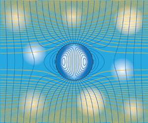
With the objective of developing theoretical predictions of the electrical conductivity of polyelectrolyte hydrogels doped with spherical cavities, the overall strategy is to compute steady-state ion fluxes for a single cavity in an unbounded hydrogel. This is undertaken within the framework of a standard electrokinetic model (O'Brien 1981) by which an equilibrium state, governed by the nonlinear Poisson–Boltzmann equation (Russel, Saville & Schowalter 1989), is perturbed by separately subjecting the cavity to a uniform electric field and a uniform pressure gradient. These solutions furnish dipole strengths of the perturbed electrostatic potential, ion concentrations and pressure, which together furnish averaged current and momentum fluxes in response to averaged gradients of electrostatic potential and pressure. The analysis is for hydrogels in which the cavity volume fraction $\phi$ is small, thus neglecting cavity–cavity interactions. Such a composite is represented schematically in figure 1.

Figure 1. (a) A dilute random array of spherical cavities (radius $R \sim 10$–$1000$ nm) is subjected to a gradient of electrostatic potential $-\boldsymbol {E}$ and/or a pressure gradient $\boldsymbol {P}$, which induce a current density $\boldsymbol {I}$ and fluid velocity $\boldsymbol {U}$. The Onsager matrix of proportionality between these macroscale gradients and fluxes is calculated on the basis of an electrokinetic model for a single cavity in an unbounded hydrogel, thus furnishing the effective conductivity for various electrode configurations. The medium bears a fixed charge density $\rho ^\infty _f$, counter-ions and added salt, furnishing a Debye screening length $\kappa ^{-1} \sim 0.1$–$1000$ nm to complement the Brinkman (hydrodynamic) screening length $\ell \sim 0.1$–$100$ nm. (b) Schematic detail of a single cavity highlighting mobile cations ($+$, green), mobile anions ($-$, red) and immobile anions ($-$, grey) fixed to the stationary polymer skeleton.

2.1. Electrokinetic model

The steady-state electrokinetic model is the one adopted by Hill (2015) for nanoparticle gel electrophoresis. It comprises the Poisson equation

(2.1)\begin{equation} {-}\epsilon \epsilon_0 \nabla^2 \psi = \rho_m + \rho_f, \end{equation}

a total of $N$ ion-conservation equations with Nernst–Plank fluxes

(2.2)\begin{equation} 0 ={-} \boldsymbol{\nabla}\boldsymbol{\cdot}\left(n_i \boldsymbol{u} - D_i \boldsymbol{\nabla} n_i - z_i e \frac{D_i}{k_B T} n_i \boldsymbol{\nabla}\psi \right) \quad (i = 1,\ldots, N) \end{equation}

and solvent momentum (inertia-free) and mass (incompressible) conservation equations

(2.3a,b)\begin{equation} 0 = \eta \nabla^2 \boldsymbol{u} - \boldsymbol{\nabla} p - \frac{\eta}{\ell^{2}} \boldsymbol{u} - \rho_m \boldsymbol{\nabla} \psi,\quad \boldsymbol{\nabla}\boldsymbol{\cdot}\boldsymbol{u} = 0, \end{equation}

where $\rho _f$ is the charge density fixed to the hydrogel skeleton, and

(2.4)\begin{equation} \rho_m = \sum_{i=1}^N z_i e n_i \end{equation}

is the net (mobile) charge density of ions in the fluid phase.

The functions to be calculated are the electrostatic potential $\psi$, the $N$ mobile-ion concentrations $n_i$, and the fluid velocity $\boldsymbol {u}$ and pressure $p$. The parameters in the foregoing equations are the thermal energy $k_B T$, dielectric permittivity $\epsilon \epsilon _0$ (assumed to be uniform due to the cavities and hydrogel being predominantly occupied by water), ion diffusion coefficients $D_i$, ion charges $z_i e$ (valence $z_i$ and fundamental charge $e$), fluid shear viscosity $\eta$ and hydrogel (Brinkman) permeability $\ell ^2$.

The permeability and fixed charged density are prescribed functions of radial distance $r$ from the cavity centre: $\ell ^{-2} = n_s(r) 6 {\rm \pi}a_s$ and $\rho _f = - \chi e n_s(r)$, where

(2.5)\begin{equation} \frac{n_s(r)}{n_s^\infty} = 1 - \frac{1}{2}\mbox{erfc}[(r - R) / \delta] \end{equation}

is the concentration of Stokes resistance centres (with radius $a_s$), and $\chi$ is the fraction of Stokes resistance centres (bearing a single negative charge). Equation (2.5) is a convenient phenomenological means to insert a spherical cavity, avoiding cumbersome boundary conditions to couple the interior and exterior domains, also enabling one to vary the sharpness of the transition. Although there are no experimental measures available, the cavities in real hydrogels likely have a more gradual transition than assumed (for simplicity) herein. All the results reported below were undertaken with $\delta = 1$ nm and cavity radii in the range $R = 1$–$1000$ nm. Accordingly, the Brinkman length undergoes a rapid variation from $\infty$ inside the cavity to a prescribed finite value in the bulk hydrogel

(2.6)\begin{equation} \ell = \frac{1}{\sqrt{n_s^\infty 6 {\rm \pi}a_s}}. \end{equation}

Note that, when $\ell$ and $\rho _f^\infty$ are considered independent variables,

(2.7)\begin{equation} \chi = \frac{-\rho^\infty_f / e}{n_s^\infty} ={-}(\rho^\infty_f / e) 6 {\rm \pi}a_s \ell^2 \end{equation}

may be (unphysically) greater than one. For example, varying $\ell$ from $0.1$ to $100$ nm with $a_s = 0.15 \times 10^{-10}$ m, $n_s^\infty$ varies from $600$ M to $0.6$ mM, whereas $-\rho ^\infty _f / e$ will be prescribed in the range $0.1$–$10$ mM. Note that these estimates of $n_s^\infty$ neglect the hydrodynamic interactions between the Stokes resistance centres, which increase the effective value of $a_s$ when their volume fraction $n^\infty _s 4 {\rm \pi}a_s^3 / 3$ is not sufficiently small. In very dense polymers, however, ion mobilities will be smaller than based on their limiting molar conductivities (as assumed herein). The dielectric constant of the hydrogel would also be smaller than the value for water (assumed herein).

The electrokinetic model, which is nonlinear, is solved by perturbing the variables from their equilibrium values, calculated with the application of either an applied pressure gradient $\boldsymbol {P} = \boldsymbol {\nabla }{p}$ as $r \rightarrow \infty$ or an electric field $\boldsymbol {E} = - \boldsymbol {\nabla } \psi$ as $r \rightarrow \infty$. More general solutions with both fields acting are obtained by linear superposition.

The equilibrium values, identified with superscripts $0$, are functions of radial position: $\boldsymbol {u}^0 = 0$ with $\psi ^0$, $n_i^0$ and $p^0$ solving the nonlinear Poisson–Boltzmann system

(2.8)$$\begin{gather} -\epsilon \epsilon_0 \nabla^2 \psi^0 = \sum_{i=1}^N z_i e n_i^0 + \rho_f, \end{gather}$$

(2.9)$$\begin{gather}0 ={-} \boldsymbol{\nabla}\boldsymbol{\cdot}\left(- D_i \boldsymbol{\nabla} n_i^0 - z_i e \frac{D_i}{k_B T} n_i^0 \boldsymbol{\nabla}\psi^0 \right) \quad (i = 1,\ldots, N), \end{gather}$$

(2.10)$$\begin{gather}0 ={-} \boldsymbol{\nabla} p^0 - \sum_{i=1}^N z_i e n_i^0 \boldsymbol{\nabla} \psi^0, \end{gather}$$

with boundary conditions

(2.11a,b)\begin{equation} \frac{\mbox{d} n_i^0}{\mbox{d} r} = 0 \quad\mbox{and}\quad \frac{\mbox{d} \psi^0}{\mbox{d} r} \rightarrow 0 \quad\mbox{at } r =0, \end{equation}

and

(2.12a,b)\begin{equation} n_i^0 \rightarrow n_i^\infty \quad \mbox{and}\quad \psi^0 \rightarrow 0 \quad\mbox{as } r \rightarrow \infty. \end{equation}

Note that bulk electroneutrality demands $\rho ^\infty _f + \rho _m = 0$ at $r = \infty$. Moreover, it is assumed that there is no external electrolyte bath, which would alter the bulk ion concentrations by inducing a non-zero Donnan potential in the hydrogel (with respect to the bath) (Doi 2013). The equilibrium solution is accomplished using finite differences with an adaptive mesh (Hill, Saville & Russel 2003) and equilibrium pressure $p^0 = - \sum _{i=1}^N z_i e n_i^0 \psi ^0$ (furnished by the equilibrium momentum equation).

Next, the equations are solved with boundary conditions for two linearly independent solutions. In this work, both solutions have

(2.13)\begin{equation} n_i \rightarrow n_i^\infty \quad \mbox{as } r \rightarrow \infty, \end{equation}

since it is assumed that there are no macroscopic ion-concentration gradients (with vanishing Donnan potential). As noted by O'Brien & Perrins (1984), this may be justified when the forcing time scale is large compared with the micro-scale relaxation times (e.g. micro-diffusion time scale $\sim R^2 / D_i$) and short enough to avoid the build-up of substantial ion-concentration gradients. For example, on the macro-scale with characteristic length $L$, the diffusion time $\tau _d \sim L^2/ D_i$ with electro-migration time $\tau _e \sim L k_B T / (|\boldsymbol {E}| |z_i| e D_i)$. Thus, with $|\boldsymbol {E}| = |\Delta V| / L$, where $\Delta V$ is the voltage across the sample, we find $\tau _e \sim \tau _d / |\Delta V|^*$ where $|\Delta V|^* = |\Delta V| |z_i| e / (k_B T)$.

One linearly independent solution comes from the application of an electric field $\boldsymbol {E}$ in the absence of a mean pressure gradient $\boldsymbol {P} = 0$

(2.14)\begin{equation} \psi \rightarrow - \boldsymbol{r} \boldsymbol{\cdot} \boldsymbol{E} \quad \mbox{as } r \rightarrow \infty. \end{equation}

As readily verified from the momentum equation, this generates a uniform far-field flow $\boldsymbol {u} \rightarrow - \boldsymbol {E} \rho ^\infty _f \ell ^2 / \eta$ as $r \rightarrow \infty$. The other linearly independent solution comes from the application of a pressure gradient $\boldsymbol {P}$ in the absence of a mean electric field $\boldsymbol {E} = 0$

(2.15)\begin{equation} p \rightarrow \boldsymbol{r} \boldsymbol{\cdot} \boldsymbol{P} \quad \mbox{as } r \rightarrow \infty, \end{equation}

which generates a uniform far-field flow $\boldsymbol {u} \rightarrow - \boldsymbol {P} \ell ^2 / \eta$ as $r \rightarrow \infty$.

Solutions of the linearized model have the general form (deduced by linearity and symmetry considerations)

(2.16)$$\begin{gather} \psi(\boldsymbol{r}) = \psi^0(r) - \boldsymbol{r} \boldsymbol{\cdot} \boldsymbol{E} + \hat{\psi}(r) \boldsymbol{e}_r \boldsymbol{\cdot} \boldsymbol{X}, \end{gather}$$

(2.17)$$\begin{gather}n_i (\boldsymbol{r}) = n_i^0(r) + \hat{n}_i(r) \boldsymbol{e}_r \boldsymbol{\cdot} \boldsymbol{X}, \end{gather}$$

(2.18)$$\begin{gather}\boldsymbol{u} ={-} \frac{\ell^2}{\eta} \boldsymbol{P} - \rho^\infty_f \frac{\ell^2}{\eta} \boldsymbol{E} + \boldsymbol{\nabla} \times \boldsymbol{\nabla} \times h(r) \boldsymbol{X}, \end{gather}$$

where $\boldsymbol {X} = \boldsymbol {E}$ or $\boldsymbol {P}$, thus solving

(2.19)$$\begin{gather} -\epsilon \epsilon_0 \nabla^2 \psi' = \rho'_m + \rho'_f, \end{gather}$$

(2.20)$$\begin{gather}0 ={-} \boldsymbol{\nabla}\boldsymbol{\cdot}\left(n^0_i \boldsymbol{u} - D_i \boldsymbol{\nabla} n'_i - z_i e \frac{D_i}{k_B T} n'_i \boldsymbol{\nabla} \psi^0 - z_i e \frac{D_i}{k_B T} n^0_i \boldsymbol{\nabla} \psi' \right) \quad (i = 1,\ldots, N), \end{gather}$$

(2.21)$$\begin{gather}0 = \eta \nabla^2 \boldsymbol{u} - \boldsymbol{\nabla} p' - \frac{\eta}{\ell^{2}} \boldsymbol{u} - \rho'_m \boldsymbol{\nabla} \psi ^0 - \rho^0_m \boldsymbol{\nabla} \psi',\quad \boldsymbol{\nabla}\boldsymbol{\cdot}\boldsymbol{u} = 0, \end{gather}$$

where

(2.22)\begin{equation} \rho'_m = \sum_{i=1}^N z_i e n'_i \end{equation}

is the perturbed mobile-ion charge density. Note that primed variables denote the perturbation from equilibrium, i.e. $(\cdot )' = (\cdot ) - (\cdot )^0$, and that continuity of the perturbed variables at the origin requires

(2.23)\begin{equation} \hat{\psi} = \hat{n}_i = h_r(r=0) = 0 \quad \mbox{at } r = 0. \end{equation}

Then the velocity, constructed from the scalar function $h(r)$ above, may be written (radial and tangential components)

(2.24)\begin{equation} \boldsymbol{u} = \left(\boldsymbol{U}_0 - 2 \frac{h_r}{r} \boldsymbol{X} \right) \boldsymbol{\cdot} \boldsymbol{e}_r \boldsymbol{e}_r + \left[ \boldsymbol{U}_0 - \left(h_{rr} + \frac{h_r}{r}\right)\boldsymbol{X} \right] \boldsymbol{\cdot} \boldsymbol{e}_\theta \boldsymbol{e}_\theta, \end{equation}

where the uniform far-field velocity

(2.25)\begin{equation} \boldsymbol{U}_0 ={-} \frac{\ell^2}{\eta} \boldsymbol{P} - \rho^\infty_f \frac{\ell^2}{\eta} \boldsymbol{E}. \end{equation}

The equations and boundary conditions are solved using finite differences with an adaptive mesh (Hill et al. 2003). The pressure is eliminated by taking the curl of the momentum equation and noting that the velocity written in terms of $h(r)$ satisfies the continuity equation. Pertinent aspects of this numerical solution are highlighted in § 2.5. First, details on how the solutions of this model are used to derive the averaged fluxes for cavity doped hydrogels are presented.

2.2. Averaged current density

The linearly independent solutions of the electrokinetic model detailed in § 2.1 provide asymptotic coefficients that are shown in this section to prescribe the averaged fluxes in a hydrogel that bears randomly distributed cavities with cavity volume fraction $\phi \ll 1$. The averaging undertaken here is inspired by the methodology of Saville (1979) for colloidal dispersions. As shown in Appendix A, this is equivalent to the ensemble averaging applied by Koch & Brady (1985) to hydrodynamic dispersion in fixed beds of spheres. Volume averaging over the entire composite is reduced to the evaluation of unconditionally convergent volume integrals that enclose a single cavity in an unbounded hydrogel. Then, following a methodology introduced by O'Brien (1981), these are transformed to surface integrals that can be expressed in terms of the dipolar disturbances of a single cavity in an unbounded hydrogel. In contrast to colloidal dispersions, the averaged current density for a cavity doped hydrogel requires explicit knowledge of the fluid-velocity disturbances.

The averaged electrical current density (steady state) is written as the volume average of the advective, electro-migrative and diffusive current fluxes

(2.26)\begin{align} \boldsymbol{I} &= \frac{1}{V} \int_{V} \sum_{i=1}^{N} z_i e \boldsymbol{j}_i \,\mbox{d}V \nonumber\\ &= \frac{1}{V} \int_{V} \sum_{i=1}^{N} \left[z_i e n_i^\infty \boldsymbol{u} - z_i e D_i \boldsymbol{\nabla}{n_i} - (z_i e)^2 \frac{D_i}{k_B T} n^\infty_i \boldsymbol{\nabla}{\psi}\right] \,\mbox{d}V \nonumber\\ &\quad + \frac{1}{V} \int_{V} \sum_{i=1}^{N} \left[z_i e \boldsymbol{j}_i - z_i e n_i^\infty \boldsymbol{u} + z_i e D_i \boldsymbol{\nabla}{n_i} + (z_i e)^2 \frac{D_i}{k_B T} n^\infty_i \boldsymbol{\nabla}{\psi}\right]\mbox{d}V, \end{align}

where the total flux of the $i$th mobile ion is

(2.27)\begin{equation} \boldsymbol{j}_i = n_i \boldsymbol{u} - D_i \boldsymbol{\nabla}{n_i} - z_i e \frac{D_i}{k_B T} n_i \boldsymbol{\nabla}{\psi}. \end{equation}

Note that the integrands are written in terms of bulk variables that yield unconditionally convergent integrals for random cavity configurations that are dilute enough for their Debye layers not to overlap (Saville 1979). This requires a cavity volume fraction $\phi \ll [1 + 1 / (\kappa R)]^{-1/3}$. Note that the velocity disturbances in the hydrogel (Brinkman medium) decay as $\boldsymbol {u}' \sim r^{-3}$, reflecting the gradient of a dipolar decay of the accompanying pressure perturbation in the far field (Brinkman 1947).

In a uniform hydrogel without cavities,

(2.28)\begin{equation} \boldsymbol{I} = \sum_{i=1}^{N} \left( z_i e n_i^\infty \boldsymbol{U} + (z_i e)^2 \frac{D_i}{k_B T} n^\infty_i \boldsymbol{E} \right), \end{equation}

where $\boldsymbol {U} = \boldsymbol {U}_0$ comprises the electro-osmotic and pressure driven terms in (2.25). With bulk electro-neutrality, the current density in a uniform (cavity free) hydrogel is

(2.29)\begin{equation} \boldsymbol{I} = \sigma_\infty \left(1 + \frac{{\rho^\infty_f}^2 \ell^2}{\sigma_\infty \eta}\right) \boldsymbol{E} + \frac{\rho^\infty_f \ell^2}{\eta} \boldsymbol{P}, \end{equation}

where

(2.30)\begin{equation} \sigma_\infty = \sum_{i=1}^{N} (z_i e)^2 \frac{D_i}{k_B T} n^\infty_i \end{equation}

is the electro-osmosis-free conductivity.

Note that the electro-migrative current density in a hydrogel for which the current is dominated by the counter-ions is $\sim \rho ^\infty _f D_i E e / (k_B T)$, and the advective/electro-osmotic current density is $\sim \rho ^\infty _f u_{eo} = {\rho ^\infty _f}^2 E \ell ^2 / \eta$. Thus, the ratio of the electro-osmotic to electro-migrative currents is

(2.31)\begin{equation} \sim \mbox{Pe}_g = \frac{u_{eo}}{D_i E e / (k_B T)} = \frac{\rho^\infty_f \ell^2 k_B T}{\eta D_i e} = 6 {\rm \pi}a_i \ell^2 \rho^\infty_f / e, \end{equation}

where $D_i = k_B T / (6 {\rm \pi}\eta a_i )$ with $a_i$ the Stokes radius of a counter-ion. This ratio may be large or small, depending on the fixed charge density and permeability, both of which will be varied systematically when the results are presented.

Now returning to the cavity filled hydrogel, (2.26) may be written

(2.32)\begin{align} \boldsymbol{I} &= \sum_{i=1}^{N} \left[ z_i e n_i^\infty \langle \boldsymbol{u} \rangle - (z_i e)^2 \frac{D_i}{k_B T} n^\infty_i \langle \boldsymbol{\nabla}{\psi} \rangle \right] \nonumber\\ &\quad + \frac{1}{V} \int_{V} \sum_{i=1}^{N} \left[z_i e (n_i^0 - n^\infty_i) \boldsymbol{u} - (z_i e)^2 \frac{D_i}{k_B T} (n_i^0 - n^\infty_i) \boldsymbol{\nabla}{\psi}' - (z_i e)^2 \frac{D_i}{k_B T} n_i' \boldsymbol{\nabla}{\psi}^0\right]\mbox{d}V, \end{align}

where $\langle \cdot \rangle$ denotes the volume average (or ensemble average). Note that the integrands in the second line vanish beyond the diffuse layer of each cavity because $n_i^0 - n^\infty _i$ and $\boldsymbol {\nabla }{\psi }^0$ are exponentially small there. It follows that the volume $V$ over which the integrals are evaluated in (2.32) can be replaced by an integral over the volume of a single cavity in an unbounded hydrogel $V'$. This amounts to replacing $V^{-1} \int _{V}$ with $n \int _{V'}$ (assuming all integrals/cavities are equal), where $n = 3 \phi / (4 {\rm \pi}R^3)$ is the cavity number density. This is equivalent to integrating the conditionally averaged fields $\langle \cdot \rangle _1$ in ensemble averaging when the dispersed phase is dilute (Hinch 1977; Koch & Brady 1985).

Having now established that the averaging in the second line of (2.32) can be evaluated in terms of unconditionally convergent integrals, we may now draw on the following identities (with $\boldsymbol {\nabla }\boldsymbol {\cdot }{\boldsymbol {u}} = \boldsymbol {\nabla }\boldsymbol {\cdot }{\boldsymbol {j}_i} = 0$) to evaluate the volume integrals from (2.26):

(2.33)\begin{equation} \int_V \boldsymbol{\nabla}{(\boldsymbol{\cdot})} \mbox{d}V \rightarrow \int_A (\boldsymbol{\cdot}) \boldsymbol{e}_r \,\mbox{d}A, \end{equation}

and

(2.34a,b)\begin{equation} \int_V \boldsymbol{j} \,\mbox{d}V \rightarrow \int_A \boldsymbol{x} \boldsymbol{j} \boldsymbol{\cdot} \boldsymbol{e}_r \,\mbox{d}A \quad \mbox{and}\quad \int_V \boldsymbol{u} \,\mbox{d}V \rightarrow \int_A \boldsymbol{x} \boldsymbol{u} \boldsymbol{\cdot} \boldsymbol{e}_r \,\mbox{d}A. \end{equation}

In this manner, the surface integrals may be evaluated using only the asymptotic far-field decay of the spatial perturbations. This avoids having to numerically evaluate volume integrals from the single cavity in an unbounded hydrogel (approximating conditionally averaged fields $\langle \cdot \rangle _1$). The volume integral in (2.32) may be written

(2.35)\begin{align} & \frac{3 \phi}{4 {\rm \pi}R^3} \int_{A} \sum_{i=1}^{N} z_i e \boldsymbol{x} \left[(n^0_i - n^\infty_i) \boldsymbol{u} - D_i \boldsymbol{\nabla}{(n^0_i + n_i')} - z_i e \frac{D_i}{k_B T} (n_i^0 \boldsymbol{\nabla}{\psi'} + n'_i \boldsymbol{\nabla}{\psi^0}) \right] \boldsymbol{\cdot} \boldsymbol{e}_r \,\mbox{d}A \nonumber\\ &\quad + \frac{3 \phi}{4 {\rm \pi}R^3} \int_{A} \sum_{i=1}^{N} z_i e \left[ D_i (n^0_i + n_i') \boldsymbol{e}_r + z_i e \frac{D_i}{k_B T} n^\infty_i (\psi' + \psi^0) \boldsymbol{e}_r \right] \mbox{d}A, \end{align}

with $A$ the area of a concentric sphere with radius $r \rightarrow \infty$ where $\psi ^0$ and $n_i^0 - n_i^\infty$ are exponentially small. Noting the respective even–odd symmetries of $n_i^0$ and $n_i'$, and $\psi ^0$ and $\psi _i'$, the total current density becomes

(2.36)\begin{align} \boldsymbol{I} &= \sum_{i=1}^{N} \left[ z_i e n_i^\infty \langle \boldsymbol{u} \rangle + (z_i e)^2 \frac{D_i}{k_B T} n^\infty_i \boldsymbol{E} \right] \nonumber\\ &\quad +\frac{3 \phi}{R^3} \sum_{i=1}^{N} \lim_{r \rightarrow \infty} \left[z_i e D_i \left \langle (n_i' - \boldsymbol{x} \boldsymbol{\nabla}{n_i'} \boldsymbol{\cdot}) \boldsymbol{e}_r \right \rangle_\theta + (z_i e)^2 \frac{D_i}{k_B T} n^\infty_i \left \langle (\psi' - \boldsymbol{x} \boldsymbol{\nabla}{\psi'} \boldsymbol{\cdot}) \boldsymbol{e}_r \right \rangle_\theta\right] r^2, \end{align}

where

(2.37)\begin{equation} \lim_{r \rightarrow \infty} \left \langle (n_i' - \boldsymbol{x} \boldsymbol{\nabla}{n_i'} \boldsymbol{\cdot}) \boldsymbol{e}_r \right \rangle_\theta r^2 = \lim_{r \rightarrow \infty} \hat{n}^E_i r^2 \boldsymbol{E} - \frac{\ell^2}{\eta} \lim_{r \rightarrow \infty} \hat{n}^U_i r^2 \boldsymbol{P} \equiv J^E_i \boldsymbol{E} - \frac{\ell^2}{\eta} J^U_i \boldsymbol{P}, \end{equation}

and

(2.38)\begin{equation} \lim_{r \rightarrow \infty} \left \langle (\psi' - \boldsymbol{x} \boldsymbol{\nabla}{\psi'} \boldsymbol{\cdot}) \boldsymbol{e}_r \right \rangle_\theta r^2 = \lim_{r \rightarrow \infty} \hat{\psi}^E_i r^2 \boldsymbol{E} - \frac{\ell^2}{\eta} \lim_{r \rightarrow \infty} \hat{\psi}^U_i r^2 \boldsymbol{P} \equiv D^E \boldsymbol{E} - \frac{\ell^2}{\eta} D^U \boldsymbol{P}. \end{equation}

Note that $\langle \cdot \rangle _\theta = \int (\cdot )\,\mbox {d}A / (4 {\rm \pi}r^2)$ denotes a directional average over the surface of a concentric sphere with radius $r$, thus identifying dipole strengths/asymptotic coefficients for the concentration ($J_i^X$), and electrostatic-potential ($D^X$) disturbances.

In the next section, the averaged fluid velocity $\langle \boldsymbol {u}\rangle$ in (2.36) is shown to be

(2.39)\begin{equation} \langle \boldsymbol{u} \rangle ={-} \frac{\ell^2}{\eta} \boldsymbol{P} - \rho^\infty_f \frac{\ell^2}{\eta} \boldsymbol{E} + \phi \frac{\ell^2}{\eta}\frac{3C^U}{R^3} \boldsymbol{P} - \phi \frac{3C^E}{R^3} \boldsymbol{E}, \end{equation}

where

(2.40)\begin{equation} C^X = \lim_{r \rightarrow \infty} h^X_r r^2 \end{equation}

are the dipole strengths/asymptotic coefficients for the pressure disturbances. This enables (2.36) to be written

(2.41)\begin{align} \boldsymbol{I} &={-} \rho^\infty_f \left[ - \frac{\ell^2}{\eta} \boldsymbol{P} - \rho^\infty_f \frac{\ell^2}{\eta} \boldsymbol{E} + \phi \frac{\ell^2}{\eta}\frac{3C^U}{R^3} \boldsymbol{P} - \phi \frac{3C^E}{R^3} \boldsymbol{E} \right] \nonumber\\ &\quad + \sigma_\infty \left[ \boldsymbol{E} + \frac{3 \phi}{R^3} D^E_e \boldsymbol{E} - \frac{\ell^2}{\eta} \frac{3 \phi}{R^3} D^U_e \boldsymbol{P} \right], \end{align}

where

(2.42)\begin{equation} D^X_e = D^X + \frac{1}{\sigma_\infty} \sum_{i=1}^{N} z_i e D_i J^X_i \end{equation}

are termed effective electrostatic dipole strengths/asymptotic coefficients. Note that the superscripts $U$ of the asymptotic coefficients above denote that the coefficient is calculated when a uniform far-field velocity $\boldsymbol {U}_0 = - \boldsymbol {P} \eta / \ell ^2$ is prescribed with $\boldsymbol {E} = 0$.

2.3. Averaged fluid momentum

In the sections above, the velocity disturbance $\boldsymbol {u}' = \boldsymbol {u} - \boldsymbol {U}_0$ decays as $r^{-3}$, so it is tempting to calculate the average in the first line of (2.32) as

(2.43)\begin{equation} \langle \boldsymbol{u} \rangle = \frac{3 \phi}{4 {\rm \pi}R^3} \int_{V} (\boldsymbol{u} - \boldsymbol{U}_0) \,\mbox{d}V + \boldsymbol{U}_0 = \frac{3 \phi}{R^3} \lim_{r \rightarrow \infty} \langle \boldsymbol{x} (\boldsymbol{u} - \boldsymbol{U}_0) \boldsymbol{\cdot} \boldsymbol{e}_r \rangle_\theta r^2 + \boldsymbol{U}_0, \end{equation}

which, from the far-field decay of $\boldsymbol {u}'$ in (2.24), furnishes

(2.44)\begin{equation} \langle \boldsymbol{u} \rangle ={-} \frac{\ell^2}{\eta} \boldsymbol{P} - \rho^\infty_f \frac{\ell^2}{\eta} \boldsymbol{E} + \phi \frac{\ell^2}{\eta} \frac{2 C^U}{R^3} \boldsymbol{P} - \phi \frac{2 C^E}{R^3} \boldsymbol{E}. \end{equation}

However, this average does not respect Onsager reciprocity, thus motivating consideration of the averaged fluid momentum equation, which, as shown below, furnishes (2.39) (with prefactor $3$ multiplying $C^X$).

According to ensemble averaging (Hinch 1977; Koch & Brady 1985), the fields $\boldsymbol {u}$, $\psi$ and $\rho _m$ above (for a single cavity in an unbounded hydrogel) become approximations of their conditionally averaged counterparts $\langle \cdot \rangle _1$, i.e. the average of $(\cdot )$ over an ensemble of dilute, random cavity configurations, conditioned on a single cavity centred at the origin. Ensemble averaging the fluid momentum equation gives

(2.45)\begin{equation} \langle \boldsymbol{\nabla} p \rangle + \langle \eta/\ell^2 \rangle \langle \boldsymbol{u} \rangle - \langle \rho_{f} \rangle \langle \boldsymbol{\nabla}{\psi}\rangle={-}\langle (\eta / \ell^2)' \boldsymbol{u}' \rangle - \langle \rho_m' \boldsymbol{\nabla} \psi' \rangle, \end{equation}

where $(\cdot )' = (\cdot ) - \langle \cdot \rangle$, not the perturbation from equilibrium $(\cdot ) - (\cdot )^0$ adopted in the sections above for the single cavity in an unbounded hydrogel. For dilute cavity doped hydrogels, the averages on the right-hand side of (2.45) may be approximated as

(2.46)\begin{equation} \langle (\eta / \ell^2)' \boldsymbol{u}' \rangle \approx n \frac{\eta}{\ell^2_\infty} \int_{r =0}^\infty \left\langle \frac{\ell^2_\infty}{\ell^2} - 1\right\rangle_1 \langle \boldsymbol{u}' \rangle_1 \,\mbox{d}\boldsymbol{r}, \end{equation}

and

(2.47)\begin{equation} \langle \rho_m' \boldsymbol{\nabla} \psi' \rangle \approx n \rho_f^\infty \int_{r=0}^\infty \left\langle \frac{\rho_m}{\rho_f^\infty} + 1 \right\rangle_1 \langle \boldsymbol{\nabla} \psi' \rangle_1 \,\mbox{d}\boldsymbol{r}, \end{equation}

where $\boldsymbol {r} = r \boldsymbol {e}_r$ is position relative to the cavity centre (based on a uniform probability of cavity centres). To avoid having to numerically evaluate these volume integrals, a means to express them in terms of the asymptotic coefficient measuring the far-field decay of $\langle p' \rangle _1$ is sought, as follows. Note that this will transform the averages $\langle \eta / \ell ^2 \rangle$ and $\langle \rho _{f}^\infty \rangle$ on the left-hand side of (2.45) to their bulk counterparts, $\eta / \ell _\infty ^2$ and $\rho _f^\infty$, respectively.

First, the volume integral in (2.46) for incompressible flow with radially varying permeability may be written

(2.48)\begin{equation} \langle (\eta / \ell^2)' \boldsymbol{u}' \rangle ={-} n \int_{r = 0}^\infty r \langle \boldsymbol{u}' \rangle_1 \boldsymbol{\cdot} \boldsymbol{e}_r \boldsymbol{e}_r \frac{\partial (\eta \ell^{{-}2})}{\partial r} \mbox{d}\boldsymbol{r}. \end{equation}

Next, by drawing on the Maxwell stress tensor (Russel et al. 1989) for a uniform dielectric $\epsilon \epsilon _0 \boldsymbol {\nabla } \psi \boldsymbol {\nabla } \psi - \epsilon \epsilon _0 \boldsymbol {\nabla } \psi \boldsymbol {\cdot } \boldsymbol {\nabla } \psi \boldsymbol {I} / 2$ (electrical stress on the medium comprising the charged polymer and fluid) and bulk electroneutrality, it can be shown that

(2.49)\begin{equation} \langle \rho_m' \boldsymbol{\nabla} \psi' \rangle ={-}\langle \rho'_f \boldsymbol{\nabla} \psi' \rangle, \end{equation}

enabling the volume integral in (2.47) to be written

(2.50)\begin{equation} \langle \rho_m' \boldsymbol{\nabla} \psi' \rangle = n \int_{r = 0}^\infty \frac{\partial \rho_f}{\partial r} \boldsymbol{e}_r \langle \psi' \rangle_1\,\mbox{d}\boldsymbol{r}. \end{equation}

To derive a more general representation of (2.45) in terms of the asymptotic coefficients $C^X$, valid for cavities with arbitrary radial permeability and radial charge-density profiles, let us now consider the single cavity in an unbounded hydrogel. Here, we will evaluate the force $\boldsymbol {F}_1$ on the fluid within a large volume $V$ that encloses the single cavity addressed in the sections above (single-cavity problem). Accordingly, this analysis adopts the previous notation by which $(\cdot )' = (\cdot ) - (\cdot )^0$ denotes the perturbation from equilibrium (not the disturbance from an average). The force, which vanishes in the absence of fluid inertia, is

(2.51)\begin{equation} \boldsymbol{F}_1 ={-} \int_V \frac{\eta}{\ell^2} \boldsymbol{u} \,\mbox{d}V + \int_A (\boldsymbol{T}_h + \boldsymbol{T}_e) \boldsymbol{\cdot} \boldsymbol{n} \,\mbox{d}A + {\int_V \rho_f \boldsymbol{\nabla}{\psi}\,\mbox{d}V}, \end{equation}

where the integral of the electrical body force $-\rho _f \boldsymbol {\nabla }{\psi }$ on the right-hand side corrects the surface integral of the Maxwell/electrical stress tensor $\boldsymbol {T}_e$ (the total electrical force on the fluid and hydrogel). In the far field, $- (\eta / \ell _\infty ^2) \boldsymbol {U}_0 - \boldsymbol {P} - \rho _f^\infty \boldsymbol {E} = 0$, so $- (\eta / \ell _\infty ^2) \boldsymbol {u}' - \boldsymbol {\nabla } p' + \rho _f^\infty \boldsymbol {\nabla }{\psi '} \sim 0$ (neglecting $O(r^{-2})$ smaller viscous shear stresses), which may be integrated (in the radial direction), giving a far-field pressure disturbance

(2.52)\begin{align} p'(\boldsymbol{r}) ={-} \int_{r}^\infty \left(\rho_f^\infty \boldsymbol{\nabla} \psi' - \frac{\eta}{\ell_\infty^2} \boldsymbol{u}' \right) \boldsymbol{\cdot} \boldsymbol{e}_r\,\mbox{d}r = \sum_{X = P,E} \left(\rho_f^\infty D^X + \frac{\eta}{\ell_\infty^2} C^X \right) r^{{-}2} \boldsymbol{X} \boldsymbol{\cdot} \boldsymbol{e}_r. \end{align}

Now, since $\boldsymbol {F}_1 = 0$ (steady state, absence of fluid inertia), (2.51) and (2.52) furnish

(2.53)\begin{align} & - \boldsymbol{U}_0 \frac{\eta}{\ell_\infty^2} \int_{r=0}^\infty \left(\frac{\ell_\infty^2}{\ell^{2}} - 1\right) \mbox{d}V - \rho_f^\infty \boldsymbol{E} \int_{r=0}^\infty \left(\frac{\rho_f}{\rho_f^\infty} - 1\right) \mbox{d}V \nonumber\\ &\qquad + \sum_{X=P,E} \left[\int_{r=0}^\infty 2 h_r^X \boldsymbol{X} \boldsymbol{\cdot} \boldsymbol{e}_r \boldsymbol{e}_r \frac{\partial (\eta \ell^{{-}2})}{\partial r} \mbox{d}V - \int_{r=0}^\infty \hat{\psi}^X \boldsymbol{X} \boldsymbol{\cdot} \boldsymbol{e}_r \boldsymbol{e}_r \frac{\partial\rho_f}{\partial r} \mbox{d}V \right] \nonumber\\ &\quad = 4 {\rm \pi}\frac{\eta}{\ell_\infty^2} \sum_{X=P,E} C^X \boldsymbol{X}. \end{align}

The integrands of the volume integrals inside the square brackets of (2.53) are equivalent to their counterparts in (2.48) and (2.50) ($\langle \boldsymbol {u}' \rangle _1 \boldsymbol {\cdot } \boldsymbol {e}_r \equiv (\boldsymbol {u} - \boldsymbol {U}_0) \boldsymbol {\cdot } \boldsymbol {e}_r = - 2 \sum _{X=P,E} h_r^X r^{-1} \boldsymbol {X} \boldsymbol {\cdot } \boldsymbol {e}_r$ and $\langle \psi ' \rangle _1 \equiv \psi ^0 + \sum _{X=P,E} \psi ^X \boldsymbol {X} \boldsymbol {\cdot } \boldsymbol {e}_r$). Therefore, multiplying (2.53) by the cavity number density $n$, and noting

(2.54a,b)\begin{align} \left\langle \frac{\eta}{\ell_\infty} \right\rangle - n \frac{\eta}{\ell_\infty^2} \int_{r=0}^\infty \left(\frac{\ell_\infty^2}{\ell^{2}} - 1\right) \mbox{d}V = \frac{\eta}{\ell_\infty^2},\quad \langle \rho_f \rangle - n \rho_f^\infty \int_{r=0}^\infty \left(\frac{\rho_f}{\rho_f^\infty} - 1\right) \mbox{d}V =\rho_f^\infty \end{align}

transforms (2.45) to (2.39).

Equation (2.39) is the same as derived by Hill (2006) for uncharged hydrogels doped with charged nanoparticles. In that case, the asymptotic coefficients $C^X$ measure the force monopole ($\boldsymbol {F}^X = - 4 {\rm \pi}C^X \boldsymbol {X} \eta / \ell ^2$) for a particle that is immobilized by mechanical contact with the hydrogel. In (2.39), the term involving $C^X$ represents a body force equal to $\boldsymbol {F}^X$ times the cavity number density $n$. Of course, (2.39) may be applied to the purely hydrodynamic limit of the model, i.e. of pressure-driven flow past a spherical cavity in a Brinkman medium. To this end, Davis & Stone (1993) ascertained the drag force by integrating the hydrodynamic traction over the surface of porous spheres (of which a cavity is a special case). Their formula for the force on a cavity is readily verified to yield the same force as furnished by the far-field decay of the velocity disturbance (measured by $C^U$ herein) according to Hill (2006): $\boldsymbol {F}^U = - 4 {\rm \pi}C^U \boldsymbol {U} \eta / \ell ^2$. Explicit formulas for $C^{U}$ (albeit without electrical influences) are provided in § 3.2. Note that Davis & Stone used the force to self-consistently determine the effective permeability of packed beds of porous spheres (not a cavity filled Brinkman medium), thus implicitly averaging the fluid velocity by an averaged momentum/force balance.

2.4. Onsager relationships

The foregoing volume averaged current density may be derived from a general Onsager principle by which the macroscopic/averaged fluxes ($\boldsymbol {I}$, $\boldsymbol {U}$) are linearly related to the macroscopic/average gradients ($-\boldsymbol {E}$, $\boldsymbol {P}$) that drive these fluxes (Doi 2013). Adopting a power-series expansion in the cavity volume fraction for all macroscopic terms, e.g. $\boldsymbol {U} = \boldsymbol {U}_0 + \phi \boldsymbol {U}_1 + \cdots$ and $\boldsymbol {I} = \boldsymbol {I}_0 + \phi \boldsymbol {I}_1 + \cdots$, the linear response may be written

(2.55) \begin{equation} \boldsymbol{U} ={-}(\ell^2 / \eta + \phi \alpha_{UP}) \boldsymbol{P} + (-\rho^\infty_f \ell^2 /\eta + \phi \alpha_{UE}) \boldsymbol{E} + O(\phi^2), \end{equation}

and

(2.56) \begin{equation} \boldsymbol{I} ={-}(-\rho^\infty_f \ell^2 / \eta + \phi \alpha_{IP}) \boldsymbol{P} + (\sigma_\infty + {\rho^\infty_f}^2 \ell^2 / \eta + \phi \alpha_{IE})\boldsymbol{E} + O(\phi^2), \end{equation}

where $\alpha _{ij}$ are (dimensional) Onsager matrix coefficients for the cavity contributions to the macroscopic fluxes. Specifically, $\phi \alpha _{UP}$ furnishes the mass flux proportional to the pressure gradient in the absence of an electric field, which is the cavity contribution to the effective hydrodynamic permeability. Similarly, $\phi \alpha _{IE}$ is the cavity contribution to the conventional electrical conductivity (when there is no pressure gradient), and $\phi \alpha _{UE} = \phi \alpha _{IP}$ is the cavity contribution to average electro-osmotic flow (in the absence of an average pressure gradient). The Onsager matrix must be symmetric to respect time-reversal symmetry of the fluctuations at equilibrium (Doi 2013). For the present problem (e.g. with no ion-concentration or temperature gradients), this demands only that the two off-diagonal terms are equal, i.e.

(2.57)\begin{equation} \alpha_{UE} = \alpha_{IP}.\quad (\mbox{Onsager reciprocity}) \end{equation}

Note that $\phi \alpha _{IP}$ furnishes the cavity contribution to the electric current from flow driven by a pressure gradient (in the absence of an electric field).

Equating the foregoing Onsager fluxes to their averaged counterparts above furnishes

(2.58a,b)$$\begin{gather} \alpha_{UP} ={-} \frac{\ell^2}{\eta} \frac{3 C^U}{R^3},\quad \alpha_{UE} ={-} \frac{3 C^E}{R^3}, \end{gather}$$

(2.59a,b)$$\begin{gather}\alpha_{IP} = \frac{\ell^2 \sigma_\infty}{\eta}\frac{3 D_e^U}{R^3} + \rho^\infty_f \frac{\ell^2}{\eta} \frac{3 C^U}{R^3},\quad \alpha_{IE} = \sigma_\infty \frac{3D_e^E}{R^3} + \rho^\infty_f \frac{3 C^E}{R^3}, \end{gather}$$

where $\alpha _{UE} = \alpha _{IP}$. As noted above, the reciprocity relation provides a valuable consistency check on the calculations of $C^X$ and $D^X$ and $J_i^X$.

To relate the current density $\boldsymbol {I}$ to measurements, there are two pertinent experimental configurations. One is conducted with zero pressure gradient, for which the ratio

(2.60)\begin{equation} \frac{I}{E} = \sigma_{P=0} = (\sigma_\infty + {\rho^\infty_f}^2 \ell^2 / \eta) (1 + \Delta \sigma_{P =0} \phi + \cdots), \end{equation}

thus defining a (dimensionless) conductivity increment

(2.61)\begin{equation} \Delta \sigma_{P = 0} = \frac{\dfrac{\rho^\infty_f}{\sigma_\infty } \dfrac{3 C^E}{R^3} +\dfrac{3 D^E_e}{R^3}}{1 + \dfrac{{\rho^\infty_f}^2 \ell^2}{ \sigma_\infty \eta}}. \end{equation}

The other is conducted with impenetrable electrodes so that there is zero average flow, for which the ratio

(2.62)\begin{equation} \frac{I}{E} = \sigma_{U=0} = \sigma_\infty (1 + \Delta \sigma_{U = 0} \phi + \cdots), \end{equation}

thus defining a conductivity increment

(2.63)\begin{equation} \Delta \sigma_{U = 0} = \frac{3 D^E_e}{R^3} + \frac{\rho^\infty_f \ell^2}{\eta}\frac{3 D^U_e}{R^3} . \end{equation}

Note that the conductivity increment counterpart for colloidal dispersions is (Saville 1979; O'Brien 1981; Hill et al. 2003)

(2.64)\begin{equation} \Delta \sigma = (\sigma / \sigma_\infty - 1) / \phi = \frac{3 D_e^E}{R^3} - M \frac{3 D_e^U}{R^3}, \end{equation}

where $M = V / E = - U / E$ is the particle electrophoretic mobility. Of course, for immobile particles ($M = 0$), the conductivity increment depends only on the effective electric-field-induced dipole strength, as is the case for ideal conducting solid composites. When we examine the results for cavity doped hydrogels, the conductivity increments will be compared with a greatly simplified analysis based on the conductivities of the cavity interior and exterior for electro-migration of mobile ions, as predicted by Donnan equilibrium between the hydrogel and cavity. This completely neglects electro-osmosis and the other diffuse-layer polarization effects captured by the full electrokinetic model.

2.5. Numerics

The numerical solution is challenging due to several disparate length scales, exemplified by the ratios $\kappa R$ and $R / \ell$, and the coupled diffusion, advection and electro-migration. Here, numerical stiffness is tackled using the method of Hill (2006) for the electrokinetics of spherical nanoparticles in hydrogels. This code, which employs finite-difference approximations and an adaptive mesh (Hill et al. 2003), was modified to solve the equations on $0 \le r \le r_{max}$. Based on Hill et al. (2003), the equations are scaled using a characteristic velocity $u^* =(k_B T / e)^2 \epsilon \epsilon _o / (\eta a)$, where $a$ is the radius of a colloidal sphere. The counterpart for the present problem is $u_c = \kappa (k_B T / e) \rho ^\infty _f \ell ^2 / \eta = u^* \kappa a (\kappa \ell )^2 \rho ^\infty _f / (2 I e)$, so $a$ becomes an arbitrary/numerical parameter/length that only affects the numerical solution via its influence on the ion Péclet numbers, for example. Of course, owing to linearity, the value of $u_c$ should not affect the physical solution. This was verified to be so, and the dimensionless quantities gleaned from the flow/pressure-driven flows herein are appropriately scaled by a factor $\kappa a$ so that their resulting $O(1)$ magnitudes are independent of $a$ (thus depending on $R$).

Numerical accuracy was tested by examining Onsager reciprocity. Here, the coefficients $C^U$ and $C^E$ of the velocity disturbances were found to be susceptible to the choice of $u_c$ (or $a$), irrespective of other numerical factors, such as the spatial discretization and the maximum radial extent of the computations, $r_{max}$, which must be very large to capture the far-field asymptotic decays of all the perturbations. The ratio of the off-diagonal Onsager coefficients $\alpha _{UE} / \alpha _{IP}$ was initially found to deviate (by a ratio of the order of one) from one. This did not have a significant or even perceptible impact on the resulting conductivity increments (under conditions where electro-osmosis is weak), but the calculation of $C^U$ and $C^E$ (and therefore the Onsager coefficients) was tremendously improved by setting $u_c$ to a very large value. The resulting calculations were then readily verified to satisfy Onsager reciprocity. This also stabilized computations for large cavities ($R \gtrsim 100$ nm), lending further confidence to the numerical accuracy of the results reported herein.

Calculations with $R / \ell \lesssim 1$ and $\kappa R \lesssim 1$ exhibited notable systematic departures of $\alpha _{UE} / \alpha _{IP}$ from one. In such cases, however, the velocity disturbances, as measured by $C^U$ and $C^E$ were very weak, and so the conductivity increments were not susceptible to numerical inaccuracies in $C^U$ and $C^E$. Furthermore, because the cavities under these conditions present vanishing disturbances, the breakdown seems to reflect numerical stiffness.

Further checks of the numerical accuracy were undertaken by comparing the Onsager coefficient $\alpha _{UP}$ for weakly charged hydrogels with exact analytical formulas derived by solving the Stokes and Brinkman equations for a spherical cavity within a continuous Brinkman medium. These formulas are provided in the results section, and are compared with the numerically calculated Onsager counterpart $\alpha _{UP}$.

Note that the maximum radial extent for the computations reported herein was set to $\kappa r_{max} = 20 \kappa R + 40$ with $10\,000$ grid points for each of the $7$ functions (potential, $4$ ion concentrations, and two scalar functions that prescribe the velocity, $h_r$ and $g = h_{rrr}$). This enabled all the scalar fields to robustly establish their asymptotic power-law decay at $r = r_{max}$. Failing to do so generally produced poor mesh convergence and a notable violation of Onsager reciprocity (as revealed by $\alpha _{UE} / \alpha _{IP}$ deviating from one).

2.6. Donnan–Maxwell model

This section begins by establishing how the bulk electrolyte composition is prescribed to be electroneutral, also establishing independent analytical calculations of the Donnan potential $\psi _D$, and cavity and hydrogel conductivities $\sigma _c$ and $\sigma _\infty$. These are used to compute what will be termed a Donnan–Maxwell conductivity increment $\Delta \sigma _{DM}$, which neglects electro-osmosis and space-charge perturbations.

While Donnan equilibrium (Doi 2013) is anticipated when the cavity radius $R$ is large compared with the Debye length $\kappa ^{-1}$, i.e. when $\kappa R \gg 1$, it will be seen that this is not sufficient for the accompanying Donnan–Maxwell conductivity to approximate the full electrokinetic model. Nevertheless, it still provides a valuable benchmark with which to interpret electro-osmosis and space-charge polarization effects emerging from the full model.

As a specific illustrative example, let us consider a four-component electrolyte, comprising H$^+$, Cl$^-$, Na$^+$ and OH$^-$ ions. Assuming, for simplicity, that the fixed charge density $\rho ^\infty _f$ is independent of the pH (i.e. a strong electrolyte), electro-neutrality in the bulk hydrogel demands

(2.65)\begin{equation} 10^{-\text{pH}} - [\mbox{Cl}^-] + [\mbox{Na}^+] - 10^{\text{pH} - 14} + \rho^\infty_f / (10^3 N_A e) = 0, \end{equation}

where $[\cdot ]$ explicitly denotes an ion concentration in $\mbox {M}=\mbox {mol}$ l$^{-1}$, and $\mbox {pH} = -\log _{10}{[\mbox {H}^+]}$ with $[\mbox {H}^+] [\mbox {OH}^-] = 10^{-14}$ M$^2$ ($N_A$ is Avogadro's number).

If the pH and $\rho ^\infty _f$ are adopted as independent variables, then $[\mbox {Na}^+]$ or $[\mbox {Cl}^-]$ may be prescribed according to the sign of

(2.66)\begin{equation} 10^{-\text{pH}} - 10^{\text{pH} - 14} + \rho^\infty_f / (10^3 N_A e), \end{equation}

thus ascertaining $[\mbox {Cl}^-]$ or $[\mbox {Na}^+]$, respectively, from the electro-neutrality condition. At $\text {pH} = 7$, for example, this identifies Na$^+$ (Cl$^-$) counter-ions for a negatively (positively) charged hydrogel.

Thus, with an electro-neutral bulk, the equilibrium electrostatic potential $\psi ^0$ decays to zero when $\kappa (r - R) \ll 1$. Inside the cavity, $\psi ^0$ increases toward (minus) the Donnan potential $\psi _D$ as $r \rightarrow 0$. In a sufficiently large cavity ($\kappa R \gg 1$), electro-neutrality requires

(2.67)\begin{equation} \sum_i^Nz_i e n_{i}^\infty \exp({z_i \psi_D e / (k_B T)}) = 0, \end{equation}

and in the bulk hydrogel,

(2.68)\begin{equation} \sum_i^Nz_i e n_{i}^\infty + \rho^\infty_f = 0. \end{equation}

Solving these furnishes the Donnan potential $\psi _D$, to which $-\psi ^0$ in a finite cavity approaches when $\kappa R \gg 1$.

For a hydrogel with a negatively charged skeleton ($\psi _D < 0$) bearing H$^+$ and Na$^+$ counter-ions and (added NaCl), the general Donnan condition above furnishes

(2.69)\begin{equation} \psi_D = \frac{k_B T}{2 e} \ln{\frac{n_{{\rm Cl}^-}^\infty + n_{{\rm OH}^-}^\infty}{n_{{\rm H}^+}^\infty + n_{{\rm Na}^+}^\infty}} = \frac{k_B T}{2 e} \ln{\frac{[\mbox{Cl}^-] + 10^{\text{pH}-14}}{10^{-\text{pH}} + [\mbox{Na}^+]}}, \end{equation}

with either (depending on the sign of $10^{-\text {pH}} - 10^{\text {pH} - 14} + {\rho ^\infty _f} / (10^3 N_A e)$)

(2.70)\begin{equation} [\mbox{Cl}^-] = [\mbox{Na}^+] + 10^{-\text{pH}} - 10^{\text{pH} - 14} + {\rho^\infty_f} / (10^3 N_A e), \end{equation}

or

(2.71)\begin{equation} [\mbox{Na}^+] = [\mbox{Cl}^-] -10^{-\text{pH}} + 10^{\text{pH} - 14} - {\rho^\infty_f} / (10^3 N_A e). \end{equation}

Note that the electrolyte conductivity in a large ($\kappa R \gg 1$) cavity is

(2.72)\begin{equation} \sigma_c = \sum_i^N(z_i e)^2 n_{i}^\infty \exp({z_i \psi_D e / (k_B T)}) \frac{D_i}{k_B T}. \end{equation}

Expressing this in terms of independent variables ${\rho ^\infty _f}$ and $[\mbox {Cl}^-]$ gives

(2.73)\begin{align} \sigma_c &= \sum_i^N (z_i e)^2 n_{i}^\infty \left(\frac{n_{{\rm Cl}^-}^\infty + n_{{\rm OH}^-}^\infty}{n_{{\rm H}^+}^\infty + n_{{\rm Na}^+}^\infty} \right)^{z_i / 2} \frac{D_i}{k_B T}, \nonumber\\ &= \frac{e^2}{k_B T}\left(n_{{\rm H}^+}^\infty D_{{\rm H}^+} + n_{{\rm Na}^+}^\infty D_{{\rm Na}^+}\right) \left( \frac{n_{{\rm Cl}^-}^\infty + n_{{\rm OH}^-}^\infty}{n_{{\rm H}^+}^\infty + n_{{\rm Na}^+}^\infty} \right)^{1 / 2} \nonumber\\ &\quad + \frac{e^2}{k_B T} \left(n_{{\rm Cl}^-}^\infty D_{{\rm Cl}^-}+ n_{{\rm OH}^-}^\infty D_{{\rm OH}^-}\right) \left(\frac{n_{{\rm H}^+}^\infty + n_{{\rm Na}^+}^\infty}{n_{{\rm Cl}^-}^\infty + n_{{\rm OH}^-}^\infty} \right)^{1 / 2}, \end{align}

or

(2.74)\begin{align} \frac{\sigma_c k_B T}{10^3 N_A e^2} &= \left([\mbox{Cl}^-] D_{{\rm Cl}^-} + 10^{\text{pH} - 14} D_{{\rm OH}^-}\right) \left( \frac{ [\mbox{Cl}^-] + 10^{\text{pH} - 14} - \frac{{\rho^\infty_f}}{10^3 N_A e}}{[\mbox{Cl}^-] + 10^{\text{pH} - 14}} \right)^{1 / 2} \nonumber\\ &\quad + \left(10^{-\text{pH}} D_{{\rm H}^+} + ([\mbox{Cl}^-] -10^{-\text{pH}} + 10^{\text{pH} - 14} -\frac{{\rho^\infty_f}}{10^3 N_A e}) D_{{\rm Na}^+}\right) \nonumber\\ &\quad \times \left( \frac{[\mbox{Cl}^-] + 10^{\text{pH} - 14}}{ [\mbox{Cl}^-] + 10^{\text{pH} - 14} - \frac{{\rho^\infty_f}}{10^3 N_A e}} \right)^{1 / 2}. \end{align}

For example, when $\mbox {pH} = 7$ with $- \rho ^\infty _f / e$ and $n_{{\rm Cl}^-}^\infty \gg 10^{-7}$ M, (2.73) reduces to

(2.75)\begin{equation} \sigma_c \approx \frac{n_{{\rm Cl}^-}^\infty e^2}{k_B T} (D_{{\rm Cl}^-} + D_{{\rm Na}^+}) \left(1 - \frac{{\rho^\infty_f}}{n_{{\rm Cl}^-}^\infty e} \right)^{1 / 2}, \end{equation}

so when there is an excess of added salt (NaCl) such that $- \rho ^\infty _f \ll n_{{\rm Cl}^-}^\infty e$, the conductivity is that of a NaCl electrolyte. On the other hand, when $- \rho ^\infty _f \gg n_{{\rm Cl}^-}^\infty e$ (counter-ion dominated hydrogel), $\sigma _c\sim [\mbox {Cl}^-]^{1/2}$, i.e.

(2.76)\begin{equation} \sigma_c \approx \frac{e^2}{k_B T} (D_{{\rm Cl}^-} + D_{{\rm Na}^+}) \left(- n_{{\rm Cl}^-}^\infty {\rho^\infty_f} / e \right)^{1 / 2}.\quad (- \rho^\infty_f \gg n_{{\rm Cl}^-}^\infty e) \end{equation}

The foregoing Donnan equilibrium provides a basis for interpreting the conductivity of cavity doped hydrogels, albeit limited to advection-free conduction in large, space-charge-free cavities. The conductivity of the hydrogel accompanying (2.75) is

(2.77)\begin{equation} \sigma_\infty \approx \frac{n_{{\rm Cl}^-}^\infty e^2}{k_B T} \left[D_{{\rm Cl}^-} + \left(1 - \frac{{\rho^\infty_f}}{n_{{\rm Cl}^-}^\infty e} \right) D_{{\rm Na}^+} \right].\end{equation}

Thus, the classical Maxwell analysis (Russel et al. 1989) for a spherical inclusion with conductivity $\sigma _c$ embedded in an unbounded continuum with conductivity $\sigma _\infty$ furnishes a Donnan–Maxwell electrostatic dipole strength

(2.78)\begin{equation} \frac{D_{DM}}{R^3} = \frac{\sigma_c / \sigma_\infty - 1}{\sigma_c / \sigma_\infty + 2}, \end{equation}

and accompanying conductivity increment

(2.79)\begin{equation} \Delta \sigma_{DM} \equiv (\sigma / \sigma_\infty - 1) / \phi = \frac{3 D_{DM}}{R^3}, \end{equation}

where

(2.80)\begin{equation} \sigma_c / \sigma_\infty = \frac{(D_{{\rm Cl}^-}/D_{{\rm Na}^+} + 1) \left(1 - \dfrac{{\rho^\infty_f}}{n_{{\rm Cl}^-}^\infty e} \right)^{1 / 2}}{D_{{\rm Cl}^-} / D_{{\rm Na}^+} + 1 - \dfrac{{\rho^\infty_f}}{n_{{\rm Cl}^-}^\infty e}}. \end{equation}

Interestingly, for a symmetrical electrolyte, such as KCl, $\sigma _c / \sigma _\infty$ would span the range $1$–$0$ as $-{\rho ^\infty _f} / (n_{{\rm Cl}^-}^\infty e) > 0$ increases from $0$ to $\infty$, so $\Delta \sigma _{DM}$ spans the range $0$ to $-3/2$. For NaCl, for which $D_{{\rm Cl}^-}/D_{{\rm Na}^+} \approx 1.5$, however, $\sigma _c / \sigma _\infty$ may be $> 1$ when $-{\rho ^\infty _f} / (n_{{\rm Cl}^-}^\infty e) \ll 1$, thus furnishing a positive increment with sufficient added salt.

As will be shown below, the dipole strength furnished by the full electrokinetic model often deviates considerably from (2.78). This reflects additional ion conduction mechanisms, namely electro-osmotic advection and, perhaps, ion diffusion at finite values of $\kappa R$. Note that the foregoing Maxwell analysis is based on the absence of a space charge (the charge is confined to the interface at $r = R$). Thus, for example, it furnishes a perfectly uniform electric field inside the cavity, whereas the full electrokinetic model often reveals a non-zero space charge inside and outside the cavity.

3. Results

The results are organized as follows. Section 3.1 briefly examines the Donnan equilibrium upon which the perturbations in following sections depend. Section 3.2 systematically examines the electric-field- and flow/pressure-driven perturbations to the electrostatic potential, ion concentrations and flow, showing how these determine the Onsager coefficients, and the effective permeability and conductivity. These results are focussed on hydrogels with a low hydrodynamic permeability ($\ell = 1$ nm) with negligible added salt ($n_{{\rm Cl}^-} = 0.01$ mM), but systematically varying the hydrogel charge density $\rho _f^\infty$ and cavity radius $R$. Having established the principal physical features emerging from the general framework, the next sub-sections briefly elaborate by examining responses with higher hydrodynamic permeability (§ 3.3, $\ell = 100$ nm), and with added salt and intermediate hydrodynamic permeability (§ 3.4, $n_{{\rm Cl}^-} = 1$ mM, $\ell = 10$ nm). Overall, these elucidate the range of qualitative responses that exist within a physically relevant parameter space. Finally, § 3.5 provides an interpretation of the conductivity of the highly charged, hierarchical ionic hydrogels synthesized by Pan et al. (2012).

3.1. Donnan equilibrium

The equilibrium potential at the cavity centre is plotted in figure 2 vs the scaled cavity radius $\kappa R$ for hydrogels with fixed charge densities the range $-\rho ^\infty _f / e = 0.1$–$10$ mM. Note that the ionic strength varies with $\rho ^\infty _f$, causing the potentials superpose when $\kappa R \ll 1$ and plateau to their respective Donnan value when $\kappa R \gg 1$. Under the conditions prevailing in figure 2 with $- \rho ^\infty _f / e = 10$ mM ($n^\infty _{{\rm Cl}^-} = 0.01$ mM), (2.69) furnishes a substantial Donnan potential (in the gel relative to a large cavity) $\psi _D \approx -3.45 k_B T / e$, which is approached for sufficiently large cavities with $\kappa R \approx 100$. With a higher electrolyte concentration $n^\infty _{{\rm Cl}^-} = 1$ mM, for example, $\psi _D \approx -1.20 k_B T / e$.

Figure 2. Scaled electrostatic potential at the cavity centre vs the scaled cavity radius $\kappa R$ for hydrogel charge densities furnishing $- \rho ^\infty _f / e = 0.1$ (blue), $1$ (red), $5$ (yellow) and $10$ (violet) mM with NaCl electrolyte ($n^\infty _{{\rm Cl}^-} = 0.01$ mM, $\text {pH} = 7$). Dashed lines are (minus) the Donnan potential, (2.69).

Further insights into the equilibrium state are gleaned from the radial electrostatic potential and ion-concentration profiles shown in figure 3. These highlight the positive equilibrium potential inside the cavity relative to the bulk hydrogel, which bears a negative fixed charge $- \rho ^\infty _f / e = 10$ mM. Note that the added concentration of salt corresponds to a bulk concentration $n^\infty _{{\rm Cl}^-} = 0.01$ mM, so with $\text {pH} = 7$, the dominant ion is Na$^+$. As shown in (b), the Na$^+$ concentration decays by almost two orders of magnitude, while the Cl$^-$ concentration increases by two orders of magnitude, so that the bulk ionic strength inside the cavity is considerably lower than in the bulk hydrogel. Given that there is no fixed charge inside the cavity ($\kappa r \lesssim 23.3$), there is an excess of positive charge (Na$^+$ ions) on the cavity side of the cavity wall, as expected from the positive equilibrium potential $\psi ^0$.

Figure 3. (a) Scaled equilibrium electrostatic potential vs scaled radial position $\kappa r$. (b) Scaled equilibrium ion concentrations vs the scaled radial position $\kappa r$: H$^+$ (blue), Cl$^-$ (red), Na$^+$ (yellow), OH$^-$ (violet). Parameters: $R = 100$ nm ($\kappa R = 23.3$), $n^\infty _{{\rm Cl}^-} = 0.01$, $- \rho ^\infty _f / e = 10$ mM, $\ell = 1$ nm.

3.2. Perturbations from equilibrium in the low-permeability limit

Now consider the electric-field- and flow/pressure-induced perturbations from equilibrium, shown in figure 4. The response to an electric field in (a) indicates an excess deficit of Na$^+$ (relative to Cl$^-$) in the direction of $\boldsymbol {E}$ (positive $x$-axis). Thus, the resulting negative (positive) charge density along the positive (negative) $x$-axis induces a negative electrostatic dipole that hinders electro-migration. It will be seen below that this manifests as a negative conductivity increment. As seen in panel (b), pressure-gradient-induced flow $\boldsymbol {U}$ along the positive $x$-axis also induces a negative electrostatic polarization, which is dominated by a deficit of Na$^+$ ions, accompanied by relatively small perturbations in the other ion concentrations. As expected from the equilibrium ion concentrations in figure 3, the polarization is dominated by the perturbations in the concentrations of Na$^+$ and Cl$^-$ at the prevailing $\mbox {pH} = 7$ and hydrogel charge density ($-\rho _f^\infty / e = 10$ mM).

Figure 4. (a) Scaled electric-field-induced perturbations to the electrostatic potential (left) and ion-concentrations (right). (b) Scaled flow/pressure-induced perturbations to the electrostatic potential (left) and ion concentrations (right): H$^+$ (blue), Cl$^-$ (red), Na$^+$ (yellow), OH$^-$ (violet). Parameters are the same as in figure 3. Log–log scaling of the axes (not shown) reveals power-law decays $\hat {\psi }^X \sim D^X r^{-2}$ and $\hat {n}_i^X \sim J_i^X r^{-2}$ as $r \rightarrow \infty$.

Iso-contours of the electric-field-induced electrostatic potential are shown in figure 5. The total perturbation in (a) highlights that electro-migration (perpendicular to the iso-contours) directs current in the hydrogel around the cavity, as expected by the relatively low conductivity/ionic strength inside. Subtracting the potential of the applied electric field $- \boldsymbol {E} \boldsymbol {\cdot } \boldsymbol {r}$, as shown in (b), details the dipolar electrostatic cavity polarization, e.g. revealing fore–aft poles that reflect space-charge perturbations at the cavity–hydrogel interface.

Figure 5. Iso-contours of the electric-field-induced electrostatic potential perturbation constructed from $\hat {\psi }^E(r)$ in figure 4(a): (a) $\psi ' = \psi - \psi ^0$ and (b) $\psi ' + \boldsymbol {E} \boldsymbol {\cdot } \boldsymbol {r}$ with $\boldsymbol {E}$ directed along the $x$-axis.

Streamlines of the flows induced by the electric field and flow/pressure gradient are shown in figure 6. When subjected to an electric field, (a) reveals recirculating flow (toroidal vortex) inside the cavity. This is driven by the electrical body force of the applied field acting on the positive equilibrium charge density at the cavity walls. While the hydrogel bears a net positive charge (in the fluid phase), owing to the counter-ions, this is hindered by hydrodynamic coupling to the hydrogel. Thus, recirculating flow is confined to the cavity. Turning to the pressure-induced flow, (b) reveals that the high hydrodynamic permeability of the cavity draws fluid from the hydrogel into the cavity. This appears to increase the tortuosity, but still decreases the overall viscous dissipation, presumably because the cavity replaces a highly dissipative Brinkman flow with pure fluid (Stokes flow). As quantified below, this manifests in an Onsager coefficient $\alpha _{UP}$ that reflects an increase in the effective hydrodynamic permeability.

Figure 6. Iso-contours of the streamfunction for the (a) electric-field- and (b) flow/pressure-induced flows accompanying figures 4–5.

Let us consider a purely hydrodynamic analysis of the Onsager coefficient $\alpha _{UP}$, which furnishes the effective hydrodynamic/Darcy permeability of cavity doped hydrogels $\ell _e^2$ when the cavity volume fraction $\phi \ll 1$

(3.1)\begin{equation} (\ell_e / \ell)^{2} = 1 + \phi \frac{\alpha_{UP}}{\ell^2 / \eta} + \cdots= 1 - \phi \frac{3 C^U}{R^3} + \cdots. \end{equation}

Coupling the steady Stokes equations inside a spherical cavity (radius $R$) to the steady solution of Brinkman's equations in the hydrogel (with Brinkman screening length $\ell$) furnishes

(3.2)\begin{equation} \frac{\alpha_{UP}}{\ell^2 / \eta} = 3 \frac{(R/\ell)^3 + 6 (R/\ell)^2 + 15 R/\ell + 15}{(R/\ell)^3 + 6 (R/\ell)^2 + 45 R / \ell + 45}. \end{equation}

As seen in figure 7(a) (dashed line), (3.2) transits from $1$ when $R / \ell \lesssim 1$ to $3$ when $R / \ell \gg 1$. This not only provides a reference for the electrokinetic model, which captures electro-viscous effects, but serves as a bounding limit of a more general hydrodynamic model with Brinkman permeabilities $\ell _c^2$ and $\ell ^2$ inside and outside the cavity, respectively. The solution of this hydrodynamic problem furnishes (from the far-field decay of the velocity and pressure disturbances)

(3.3)\begin{equation} \frac{\alpha_{UP}}{\ell^2 / \eta} ={-}3 \left[ (\ell / \ell_c)^2 - 1 \right] \frac{A \tanh (R / \ell_c) + B R / \ell_c}{C \tanh (R / \ell_c) + D R / \ell_c}, \end{equation}

where

(3.4)$$\begin{gather} A = K_c^2 K - 3K_c^2 / K + 3K - 3K_c^2/ K^2 + 3, \end{gather}$$

(3.5)$$\begin{gather}B = K_c^2 + 3K_c^2 / K - 3K + 3K_c^2 / K^2 - 3, \end{gather}$$

(3.6)$$\begin{gather}C = 2K_c^4 / K + K_c^2K - 3K_c^2 / K + 3K - 3 K_c^2 / K^2 + 3, \end{gather}$$

(3.7)$$\begin{gather}D = 2K_c^4/ K^2 + K_c^2 + 3K_c^2 / K - 3 K + 3K_c^2 / K^2 - 3. \end{gather}$$

Figure 7. Hydrodynamic permeability according to analytical hydrodynamic theory: (a) scaled Onsager coefficient $\alpha _{UP} / (\ell ^2 / \eta )$ from (3.3) for uniform pressure-driven flow past a Brinkman sphere/cavity (permeability $\ell ^2_c$) embedded in a Brinkman medium (permeability $\ell ^2$): $R / \ell _c = 0.01$, $0.03$, $0.1$, $0.3$, $1$, $2$, $4$, $8$, $16$, $32$, $64$, $128$ (top to bottom). Dashed line is the Stokes–Brinkman equation (3.2) (empty cavity), and the dashed-dotted line is (3.8) (impenetrable cavity). Positive (negative) values of $\alpha _{UP}$ indicate conditions that increase (decrease) the permeability of the medium with permeability $\ell ^2$. (b–e) Streamlines for representative permeability contrasts (from Brinkman's equations with continuous velocity and stress at $r = R$).

Note that (3.2) is readily verified to be consistent with the drag force independently derived by Davis & Stone (1993) from the traction acting on the cavity surface. Equation (3.3), which is its more general counterpart, is plotted vs $K = R / \ell$ for fixed values of $K_c = R / \ell _c$ in figure 7(a) (solid lines). Crossing of the ordinate identifies zero permeability contrast, i.e. $\ell = \ell _c$. The impenetrable-cavity limit, achieved as $R / \ell _c \rightarrow \infty$, is readily obtained from the pressure dipole in Brinkman's calculation (Brinkman 1947) of the drag force on a sphere embedded in a porous/Brinkman medium (dash-dotted line)

(3.8)\begin{equation} \frac{\alpha_{UP}}{\ell^2 / \eta} ={-} \frac{3}{2} \left[1 + \frac{3}{R / \ell} + \frac{3}{(R /\ell)^2} \right]. \end{equation}

Equation (3.3) bridges the bounds set by (3.2) and (3.8). As the streamlines in (b–e) demonstrate, low-permeability cavities (left) direct streamlines around them, tending to decrease the permeability of the composite ($\alpha _{UP} < 0$), whereas high-permeability cavities (right) draw streamlines into them, tending to increase the composite permeability ($\alpha _{UP} > 0$). These inferences are consistent with the analysis of Grosan, Postelnicu & Pop (2010), who computed the streamlines for several similar flows (seemingly unaware of Davis & Stone 1993), but did not evaluate the force/dipole strengths underlying (3.3).

The cavity contributions to the Onsager coefficients, constructed from the foregoing electric-field- and flow/pressure-induced perturbations, are shown in figure 8. Note that $R / \ell \gg 1$, so $\alpha _{UP} \approx 3 \ell ^2 / \eta$ is practically independent of the hydrogel charge, i.e. electro-viscous effects are weak and largely independent of the cavity radius, whereas the other two independent Onsager coefficients $\alpha _{IE}$ and $\alpha _{IP} = \alpha _{UE}$ vary much more significantly with the hydrogel charge and cavity size. As expected based on the negative electrostatic polarization, $\alpha _{IE}$ is negative here, manifesting in a negative conductivity increment for hydrogels with low permeability ($\ell = 1$ nm).

Figure 8. Scaled Onsager coefficients $\alpha _{UP} / (\ell ^2 / \eta )$ (solid), $\alpha _{IE} / (\sigma _\infty + {\rho _f^\infty }^2 \ell ^2 / \eta )$ (dashed) and $\alpha _{IP} / (-\rho _f^\infty \ell ^2 / \eta ) = \alpha _{UE} / (-\rho _f^\infty \ell ^2 / \eta )$ (dash-dotted) accompanying results presented in figures 3–6: $-\rho ^\infty _f / e = 0.1$ (blue), $1$ (red), $5$ (yellow) and $10$ (violet) mM. Other parameters: $\ell = 1$ nm, NaCl electrolyte ($n^\infty _{{\rm Cl}^-} = 0.01$ mM, $\text {pH} = 7$). Black dashed line is the Stokes–Brinkman equation (3.2) for $\alpha _{UP} / (\ell ^2 / \eta )$.

Of particular interest in figure 8 is the magnitude and changing sign of $\alpha _{IP} = \alpha _{UE}$ (dashed lines), which are scaled so that positive (negative) values correspond to cavities that enhance (hinder) electro-osmotic flow in the bulk hydrogel ($\boldsymbol {U} = -\rho _f^\infty \boldsymbol {E} \ell ^2 / \eta$). By Onsager reciprocity, these also correspond to an enhancement (hindering) of the current driven by pressure-induced flow ($\boldsymbol {I} = \rho ^\infty _f \boldsymbol {P} \ell ^2 / \eta$). Enhancement is favoured by small cavities in weakly charged gels, reflecting a weaker perturbation of the flow (low tortuosity). Conversely, hindering of the flow or current by large cavities in highly charged gels reflects flow perturbations that manifest as internal recirculation.

The two conductivity increments defined by (2.60) and (2.62), and which accompany the Onsager coefficients in figure 8, are shown in figure 9. Because the hydrogel permeability is low, the increments are very similar, reflecting principally the electric-field-induced electrostatic polarizability (as measured by $D^X$, not shown). This is also evident from the conductivity deduced by the Donnan–Maxwell theory leading to (2.78) (dashed lines). The closest correspondence between the full model and the Donnan–Maxwell approximation occurs for the largest cavities in the most highly charged hydrogels (under conditions of zero mean flow), as seen in (b). While large cavities bring the equilibrium state closer to Donnan equilibrium (homogeneous cavity and hydrogel), as does increasing the hydrogel charge (decreasing the Debye layer thickness, $\kappa ^{-1}$), increasing the cavity radius also increases the cavity Péclet number, making the polarization susceptible to electro-osmotic advection.

Figure 9. Conductivity increments derived from the Onsager coefficients in figure 8: $- \rho ^\infty _f / e = 0.1$ (blue), $1$ (red), $5$ (yellow) and $10$ (violet) mM. Solid lines are the full electrokinetic model, and dashed lines are the Donnan–Maxwell equation (2.78).

3.3. Perturbations from equilibrium in the highly permeable limit

Having now examined the general methodology and some illustrative results emerging from the model, let us now consider increasing the hydrodynamic permeability of the hydrogel. To emphasize the physical consequences, from a qualitative perspective, the results are presented with a very large hydrodynamic screening length ($\ell = 100$ nm). This brings the results into a regime where $\ell / R$ is at least of the order of one, so that we may reasonably expect hydrodynamic influences to be more significant than above.

As shown in figure 10, the scaled Onsager coefficients now vary considerably with the hydrogel charge and cavity radius. Interestingly, and perhaps surprisingly, cavities decrease the hydrodynamic permeability. This electro-viscous effect is strongest for small, highly charged cavities. However, there is a notable maximum (in the magnitude) with respect to $R$, and this systematically shifts according to the magnitude of $\rho _f^\infty$. When replotting the Onsager coefficients vs $\kappa R$ (not shown), the maxima are seen to occur when $\kappa R \sim 5$, qualitatively similar to the maximum electro-viscous drag on charged colloidal spheres (Hill & Ostoja-Starzewski 2008).

Figure 10. Scaled Onsager coefficients $\alpha _{UP} / (\ell ^2 / \eta )$ (solid), $\alpha _{IE} / (\sigma _\infty + {\rho _f^\infty }^2 \ell ^2 / \eta )$ (dashed) and $\alpha _{IP} / (-\rho _f^\infty \ell ^2 / \eta ) = \alpha _{UE} / (-\rho _f^\infty \ell ^2 / \eta )$ (dash-dotted), as shown in figure 8, but for hydrogels with $\ell = 100$ nm: $- \rho ^\infty _f / e = 0.1$ (blue), $1$ (red), $5$ (yellow) and $10$ (violet) mM. Black dashed line is the Stokes–Brinkman equation (3.2) for $\alpha _{UP} / (\ell ^2 / \eta )$.

Streamlines of the electric-field-induced flow (and the accompanying electrostatic-potential perturbation) are shown in figure 11 for cavities with radius $R =50$ (a) and $200$ nm (b). Increasing $R / \ell$ causes the flow in the hydrogel to separate from flow within the cavity. Note that the flow/pressure-induced streamlines (not shown) are (to the eye) the same as shown here for the electric-field-induced flow. This suggests that the internal flow is controlled by viscous coupling to the external flow. Interestingly, the electrostatic polarization is very strong, as evidenced by the electrostatic-potential disturbance inside the cavity significantly distorting the applied electric field in the surrounding hydrogel. This disturbance is especially strong for the example with $\ell / R = 2$ ($R = 50$ nm), suggesting that, under these conditions, the advective contribution to the ion fluxes plays a significant role in the cavity polarization.

Figure 11. Electric-field-induced streamlines (left) and iso-contours of the (total) electrostatic-potential perturbation (right). Parameters: $n^\infty _{{\rm Cl}^-} = 0.01$ mM ($\mbox {pH} = 7$), $- \rho ^\infty _f / e = 10$ mM, $\ell = 100$, $R = 50$ nm (a) and $200$ nm (b). Note that the streamlines for the flow/pressure-induced flow are the same as for the electric-field-induced flow. Streamlines inside the cavity have a smaller separation of the streamfunction than outside the cavity.

The role of advection in polarizing the cavities is highlighted by the conductivity increments shown in figure 12. Interestingly, these take very large negative values (for smaller cavities in highly charged hydrogels) in the absence of an average pressure gradient, as seen in (a). However, they revert to large positive values (for larger cavities in highly charged hydrogels) in the absence of an average flow, as seen in (b). The large negative conductivity increments in (a) reflect a strong electrostatic polarization from electro-osmosis that is unimpeded by an adverse pressure gradient. In (b), however, the positive conductivity increments seem to reflect a net (positive) cavity polarization that must be attributed to the back flow required to maintain zero net flow.

Figure 12. Conductivity increments (defined by (2.60) and (2.62)) accompanying the scaled Onsager coefficients in figure 10: $- \rho ^\infty _f / e = 0.1$ (blue), $1$ (red), $5$ (yellow) and $10$ (violet) mM. Solid lines are the full electrokinetic model, and dashed lines are the Donnan–Maxwell equation (2.78).

The qualitative similarity of $\Delta \sigma _{P =0}$ in figure 12(a) to the Onsager coefficients in figure 10 suggests that the conductivity is dominated by the contribution from $\alpha _{IE}$, which depends on a weighted sum of $D_e^E$ and $C^E$. Note that $\Delta \sigma _{P =0}$ does not correlate entirely with the electrostatic dipole ($D_e^E$), so the advective contribution coming from the velocity disturbance ($C^E$) is significant. Note that the qualitative form of $\Delta \sigma _{U =0}$ in figure 12(b) bears closer resemblance to the electrostatic dipole $D_e^U$ (not shown), again suggesting that the electrical polarization is dominated by pressure-driven back flow when the electrodes are blocked. Moreover, the flow/pressure-induced electrostatic polarization is qualitatively the same as the electric-field-induced disturbances shown in figure 11 (without the contribution of the applied field $- \boldsymbol {E} \boldsymbol {\cdot } \boldsymbol {r}$).

3.4. Perturbations from equilibrium at intermediate permeability with added salt

Results for hydrogels bearing the same fixed charged densities as in the examples above, but now with a significant amount of added salt ($n^\infty _{{\rm Cl}^-} = 1$ mM) and an intermediate hydrodynamic permeability ($\ell = 10$ nm) are shown in figures 13 and 14. Added salt increases the conductivity of the cavity and hydrogel domains, also reducing the Donnan potential, which reduces the conductivity contrast between the cavity and hydrogel domains. Whereas one might expect the weaker concentration/conductivity contrast to diminish the conductivity increments, this is not the case, again owing to electro-osmosis.

Figure 13. Scaled Onsager coefficients $\alpha _{UP} / (\ell ^2 / \eta )$ (solid), $\alpha _{IE} / (\sigma _\infty + {\rho _f^\infty }^2 \ell ^2 / \eta )$ (dashed) and $\alpha _{IP} / (-\rho _f^\infty \ell ^2 / \eta ) = \alpha _{UE} / (-\rho _f^\infty \ell ^2 / \eta )$ (dash-dotted): $- \rho ^\infty _f / e = 0.1$ (blue), $1$ (red), $5$ (yellow) and $10$ (violet) mM. Other parameters: $\ell = 10$ nm, NaCl electrolyte ($n^\infty _{{\rm Cl}^-} = 1$ mM, $\text {pH} = 7$). Black dashed line (overlapping the blue solid line) is the Stokes–Brinkman equation (3.2) for $\alpha _{UP} / (\ell ^2 / \eta )$.

Figure 14. (a,b) Con ductivity increments (defined by (2.60) and (2.62)) accompanying the scaled Onsager coefficients in figure 13. Solid lines are the full electrokinetic model, and dashed lines are the Donnan–Maxwell equation (2.78). (c,d) Scaled electrostatic dipole strengths: $D_e^X$ (effective dipole, see (2.42), solid lines), $D^X$ (electrostatic dipole, dashed lines).

As shown in figure 13, the electrokinetic model for the hydrogel with the weakest charge (blue lines) furnishes a permeability increment ($\alpha _{UP}$) that agrees exactly with the Stokes–Brinkman hydrodynamic calculation, (3.2) (black dashed line). The effective hydrodynamic permeability not only increases with the cavity volume fraction, since $\alpha _{UP} > 0$ (solid lines), but also varies significantly with the cavity radius and hydrogel charge. Here, strong electro-viscous effects (as highlighted in § 3.3) arising from cavity polarization are suggested by the effective hydrodynamic permeability decreasing with increasing charge (compare with the charge-invariant permeability in figure 8).

Whereas the Donnan–Maxwell theory predicts relatively small, negative conductivity increments, due to the weak conductivity contrast between the cavities and hydrogel, the conductivity increments shown in figure 14 deviate significantly from the Donnan–Maxwell theory, particularly when there is zero mean flow. As highlighted above, the pressure-induced back flow manifests in positive increments in highly charged hydrogels, increasing with the cavity size. The distinctly different magnitudes of the (scaled with $R^3$) electrostatic dipole strengths ($D_e^X / R^3$) in (c,d) [from the conductivity increments in (a,b)] again highlight the role of advection.

3.5. Experimental interpretation

Before concluding, let us consider the hierarchical hydrogels of Pan et al. (2012). Using the characteristic compositions (highlighted in the introduction), the maximum fixed charge density may be crudely estimated from the water ($w$) fraction $\approx 93$ wt% and molar ratios of aniline monomer ($an$) and phytic acid ($pa$) $R = N_{an} / N_{pa}$ in the range 2:1 to 7:1. From the molecular weights of the components ($am, pa, w$), we have

(3.9)\begin{equation} 0.93 \approx \frac{1}{1 + 18 / (93 N_{an} / N_w + 660 N_{pa} / N_w)}, \end{equation}

with a maximum of $6$ negative fixed charges for each phytic acid molecule. Thus, the maximum fixed charge density is

(3.10)\begin{equation} {-}\rho_f^\infty \lesssim \frac{6 e N_{pa}}{N_w 18 / \rho_w}, \end{equation}

where $\rho _w \approx 0.97$ g cm$^{-3}$, giving

(3.11)\begin{equation} {-}\rho_f^\infty / e \lesssim (0.34 - 0.53)\,\text{mol}\,{\rm l}^{{-}1}. \end{equation}

Next, assuming the counter-ions are H$_3$O$^+$, the conductivity based on the molar conductivity of H$_3$O$^+$ (${\approx }350$ S cm$^{2}$ mol$^{-1}$, equivalent to $D_{{\rm H}^+} \approx 9.3 \times 10^{-9}$ m$^2$ s$^{-1}$ at $T = 298$ K) alone is estimated by (2.30) to be, e.g. $\sigma _\infty \approx 0.17\,\text {S}\,\text {cm}^{-1}$, when $R = 3$. Note that dried, compressed polyaniline was reported by Pan et al. to have an electronic conductivity $0.23$ S cm$^{-1}$. Therefore, in the swollen hydrogel state, we might expect an additive electronic contribution to the hydrogel conductivity $\lesssim (1 - 0.93) \times 0.23 = 0.016$ S cm$^{-1}$ (assuming a volume fraction $\lesssim 0.07$), giving a total (ionic plus electronic) conductivity

(3.12)\begin{equation} \sigma^\infty \lesssim 0.17 + 0.016 = 0.19\,\text{S}\,\text{cm}^{{-}1}. \end{equation}

For such a gel, Pan et al. reported a conductivity $0.11$ S cm$^{-1}$, which is $\approx$42 % lower than predicted here on the basis of complete ionization ($6$ strong acid moieties) without micro-scale electrokinetic effects or coupling of ionic- and electronic-conduction mechanisms.

Pan et al. (2012) claimed their value as a record high, noting others as having registered values in the range $0.1$–$10$ mS cm$^{-1}$. Thus, if such a high value can indeed be attributed to the hierarchical micro-structure, then it may reflect the net result of (i) partial ionization and hindered ion mobility decreasing the conductivity – both of which are plausible given the high charge densities suggested by (3.11) – and (ii) micro-scale electrokinetic effects increasing the conductivity – via a positive conductivity increment, as predicted for highly charged gels in figures 12(b) and 14(b). All these factors (including the coupling of the ionic and electronic conduction) clearly need to be carefully considered in designing an experimental program that is capable of accurately correlating conductivity and microstructure. The theory advanced herein provides a rational basis for such a program.

4. Summary and conclusions

A theoretical study of transport in charged hydrogels containing spherical cavities has been undertaken to ascertain how micro-scale inhomogeneity affects the electrical conductivity, albeit under quasi-steady conditions. On the basis of an electrokinetic model for a spherical cavity in an unbounded, charged hydrogel – modelled as a Brinkman medium with a prescribed hydrodynamic permeability and fixed charge density – the fluid momentum and charge fluxes were averaged to elucidate their linear dependence on the averaged gradients of electrostatic potential and pressure. The linear (matrix) relationship satisfied Onsager reciprocity, and the principal Onsager coefficients derived from the electrokinetic model were used to construct effective conductivities under (i) zero-pressure-gradient and (ii) zero-flow conditions. The full electrokinetic model was complemented with a substantially simplified model (termed a Donnan–Maxwell theory), neglecting space-charge perturbations and electro-osmotic flow. Exact solutions of Brinkman's model were also obtained, furnishing the effective hydrodynamic permeability of cavity doped hydrogels, albeit in the absence of charge effects at low cavity volume fraction.

In general, electro-osmosis was found to have a significant impact on the electrical conductivity, thus limiting the quantitative and qualitative capabilities of the Donnan–Maxwell analysis, even for cavities for which the Debye length is very small compared with the cavity radius. Electromigration and electro-osmotic advection act in concert to impart electrical polarization and electro-viscous effects.

The model provides guidance on how boundary conditions and the microstructure of polyelectrolyte hydrogels affect ion transport and osmosis in charged porous membranes. For example, electro-osmosis in highly charged and permeable hydrogels imparts a large negative conductivity increment with open boundary conditions (zero pressure gradient), and a large positive conductivity increment with closed boundary conditions (zero flow). These both reflect flow-induced electrical polarization (space-charge density perturbation). With open boundary conditions, cavities are polarized in a manner that attenuates the applied electric field, thus hindering ion conduction. With closed boundaries, however, the electro-osmotic back flow may impart a polarization that accentuates the applied electric field, thus enhancing conduction. Note also that space-charge density perturbations arising from flow in the absence of an applied electric field decrease the effective hydrodynamic permeability relative to that predicted on purely hydrodynamic grounds, i.e. (3.2) and (3.3). This electro-viscous effect is maximized when the Debye length (depending on the counterion concentration) is of the order of the cavity radius.

The present theory is based on steady state, which may be challenging to realize in practice. Thus, future advances should address the dynamic response, i.e. the response to an oscillatory electric field, which is how electrical conductivity measurements are typically undertaken (at kilohertz frequencies). Such a theory would predict a frequency-dependent complex conductivity, thus providing a quantitative interpretation of dielectric spectroscopy. On the other hand, the present steady-state analysis may still be relevant to the relatively slow macroscale dynamics of devices (depending on their characteristic length).

Although Onsager reciprocity was verified for all the results presented, there were found exceptional regions of the parameter space (of limited physical significance) where reciprocity broke down, namely cavities with $R / \ell \lesssim 1$ and $\kappa R \lesssim 1$. It seems plausible that this may reflect numerical stiffness, since the cavities under these conditions present vanishing electrostatic and hydrodynamic disturbances to an otherwise perfectly uniform hydrogel.

Finally, it should be noted that the model developed herein is readily extended to hydrogel filled cavities, providing a foundation for understanding the conductivity and hydrodynamic permeability of microgel doped hydrogels (Latreille et al. 2019). Microgels are nano-scaled spherical hydrogels that could be dispersed in a contrasting pre-gel solution, thus providing independent control of the charge and permeability contrast on micro- and macro-scales. Such materials may be beneficial for membrane-based technologies and micro-actuators where the internal driving force is by ionic charge redistribution (Kim, van den Berg & Crosby 2021).