Integral methods for friction decomposition and their extensions to rough-wall flows

Abstract

A primary objective of integral methods, such as the momentum integral method, is to discern the physical processes contributing to skin friction. These methods encompass the momentum, kinetic energy and angular momentum integrals. This paper reformulates existing integrals based on the double-averaged Navier–Stokes equations, and extends their application to flows over rough walls. 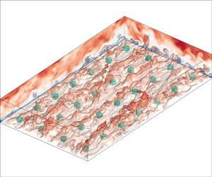Our derivation yields distinct decompositions for the bottom-wall viscous friction coefficient, denoted as $C_S$, and the roughness element drag coefficient $C_R$. The decompositions comprise three terms: a viscous term, a turbulent term and a roughness (dispersive) term – regardless of the flow configuration, be it channel or boundary layer. Notably, when these integrals are evaluated for laminar flow scenarios, only the viscous term remains significant. In addition, we elucidate the spatial distributions of the terms within these decompositions. To demonstrate the practicality of our formulations, we apply them to analyse data from direct numerical simulations of turbulent half-channel flows. These flows feature aligned and staggered cubical roughness at various packing densities. Our analyses, based on kinetic-energy-oriented decompositions, reveal that when the surface coverage density $\lambda _p$ is small, the dominant terms within the decompositions are the viscous and turbulent terms. With increasing $\lambda _p$, the viscous dissipation term decreases, while the turbulent production term increases and then decreases. These variations arise from a subdued near-wall cycle and the development of a shear layer at the height of the cubes.

1. Motivation

Pioneered by Fukagata, Iwamoto & Kasagi (2002), integral methods and decompositions of skin friction have been employed by many as diagnostic tools in their data analyses. These analyses have subsequently led to new insights into the physical processes that contribute to the generation of skin friction. This paper explores alternative formulations of the existing integrals and decompositions for flows above smooth surfaces, and extensions of these integrals and decompositions for flows above rough surfaces. Considering the successes of the integral methods thus far (Fukagata, Iwamoto & Hasegawa 2024), extending the existing methods to previously unexplored flow scenarios promises new insights, and such endeavours should need no further motivation. This is particularly true for rough-wall boundary layers, which are common in fluid engineering (Jiménez 2004; Flack & Schultz 2010; Chung et al. 2021). In this first section, we discuss two considerations that motivate the exploration of alternative integrals for smooth walls and the need for new formulations for rough walls. In §§ 2 and 3, we will summarize the equations and review prior integral methods in greater detail.

The first consideration involves distinguishing between effects that are internal and external to the flow. A theory may focus exclusively on effects that are internal or external. As an illustrative example, we examine Kármán's integral (Schlichting & Gersten 2017). The integral reads

(1.1)\begin{equation} \frac{\tau_w}{\rho U_r^2}=\frac{1}{U_r^2}\,\frac{\partial }{\partial t}(U_r\delta_1)+ \frac{\partial \delta_2}{\partial x_1} + \frac{2\delta_2+\delta_1}{U_r}\, \frac{\partial U_r}{\partial x_1}+\frac{v_w}{U_r}. \end{equation}

Here, $\tau _w$ is the wall shear stress, $U_r$ is a reference velocity, $\delta _1$ and $\delta _2$ are the displacement and momentum thickness height, $v_w$ is the blowing/suction velocity at the wall, and $x_1$ is the streamwise coordinate. The equation gives the force balance. It focuses on processes that are external to the boundary layer: given a control volume, the terms on the right-hand side represent external momentum fluxes to the boundary layer. Notice that their values depend on the frame of reference. Equation (1.1) is formally a decomposition of the skin friction. However, such decomposition provides little information on the processes that contribute to the generation of skin friction – terms such as the Reynolds shear stress that represents the effect of turbulence are absent.

We now turn to the integral methods. Here, we take the momentum integral in Fukagata et al. (2002) as an illustrative example. The derivation of their integral begins with the mean streamwise momentum equation

(1.2)\begin{equation} \frac{\partial }{\partial x_3} \left( \nu\,\frac{\partial \bar{u}_1}{\partial x_3} - \overline{u_1'u_3'} \right)=I_0 + \frac{1}{\rho}\,\frac{\partial \bar{p}}{\partial x_1} + \frac{\partial \bar{u}_1}{\partial t}, \end{equation}

where $x_1$ and $x_3$ are the streamwise and wall-normal coordinates, $u_1$ and $u_3$ are the instantaneous velocities in the $x_1$ and $x_3$ directions, $p$ is pressure, $\bar {\cdot }$ denotes time average, $\overline {u_1'u_3'}$ is the Reynolds shear stress, $\nu$ is viscosity, $\rho$ is density, and $I_0$ is a term that contains the streamwise convection term and the streamwise diffusion term:

(1.3)\begin{equation} I_0 = \frac{\partial \overline{u_1 u_1}}{\partial x_1} + \frac{\partial \bar{u}_1 \bar{u}_3}{\partial x_3} - \nu\,\frac{\partial^2 \bar{u}_1}{\partial x_1^2}. \end{equation}

Integrating the above mean momentum equation, one gets the following decomposition of the skin friction coefficient (henceforth referred to as FIK):

(1.4)\begin{align} C_f &= \frac{4(1-\delta_1)}{Re_\delta}+4\int_{0}^1\left(1-\frac{x_3}{\delta}\right) \frac{-\overline{u_1'u_3'}}{U_\infty^2}\,{\rm d} \frac{x_3}{\delta} \nonumber\\ &\quad -\frac{2\delta}{U_\infty^2} \int_{0}^{1}\left(1-\frac{x_3}{\delta}\right)^2 \left(I_0+\frac{1}{\rho}\,\frac{\partial \bar{p}}{\partial x_1}+ \frac{\partial \bar{u}_1}{\partial t}\right){\rm d}\frac{x_3}{\delta}. \end{align}

In this equation, $C_f = \tau _w/(0.5\rho U_\infty ^2)$ and $Re_\delta =U_\infty \delta /\nu$, $U_\infty$ is the freestream velocity, and $\delta$ is the boundary layer thickness. We examine the terms on the right-hand side of (1.4). The first two terms are the results of viscous diffusion and turbulent transport. These two terms do not appear in Kármán's integral and are internal to the boundary layer. They redistribute but do not inject or remove momentum from the boundary layer. The last term contains pressure gradient, flow acceleration/deceleration, and terms that are the result of the flow's evolution in the stream direction. It contains external fluxes, which contribute to the overall force balance. Following the discussion above, it was argued that the integral method would be more elegant if it contained only internal, Galilean-invariant terms. The above viewpoint was enunciated in Gao & Wu (2019) and Aghaei-Jouybari et al. (2022). The discussions in Fukagata et al. (2002) and Elnahhas & Johnson (2022) are also in line with the logic above, although the argument was less explicit.

To further illustrate this point, we apply the FIK integral to a laminar channel flow. Since the flow is laminar, $\overline {u_1'u_3'}=0$, $I_0=0$ and $\partial \bar {u}_1/\partial t=0$. It follows that (1.4) reduces to

(1.5)\begin{equation} C_f = \frac{4}{Re_b} - \frac{2}{3}\,\frac{\delta}{U_b^2}\,\frac{1}{\rho}\,\frac{\partial \bar{p}}{\partial x_1}, \end{equation}

where $C_f = \tau _w/(0.5\rho U_b^2)$ and $Re_b = U_b \delta /\nu$, $U_b$ is the bulk velocity, and $\delta$ is the half-channel height. The laminar channel friction coefficient is known and is $C_f = 6/Re_b$. Equation (1.5) contains an internal term, i.e. the first term, and an external term, i.e. the second term. The equation suggests that $2/3$ of the skin friction in a laminar channel is due to viscosity, and $1/3$ is due to the imposed pressure gradient, which is not physical. To resolve this issue, one can invoke the following force balance (see (5)–(8) in Fukagata et al. 2002):

(1.6)\begin{equation} -\tau_w/\rho = \int_0^\delta \left( I_0 + \frac{1}{\rho}\,\frac{\partial \bar{p}}{\partial x_1} + \frac{\partial \bar{u}_1}{\partial t} \right) {\rm d}\kern0.7pt x_3. \end{equation}

By performing the operation

(1.7)\begin{equation} \int_0^\delta \int_0^{x_3} \int_0^{x_3} \left({\rm Eq.}(1.2) - \alpha\,\frac{1}{\delta}\,{\rm Eq.}(1.6)\right) {\rm d}\kern0.7pt {x_3}\,{\rm d}\kern0.7pt {x_3}\,{\rm d}\kern0.7pt {x_3}, \end{equation}

and taking $\alpha =1$, one arrives at

(1.8)\begin{equation} C_f = \frac{6}{Re_b} \end{equation}

for laminar channel flow. Equation (1.8) contains one internal term only. It suggests that the skin friction in a laminar channel is due to the viscosity, which is the right-hand side.

Equation (1.7) also alludes to a longstanding issue of the integral methods. Because both (1.2) and (1.6) are exact, $\alpha$ in (1.7) is a free parameter, leading to ambiguity in the derivation. For example, Fukagata et al. (2002) took $\alpha =1$ to eliminate the pressure gradient force for channel, but took $\alpha =0$ and kept the pressure gradient and other external momentum fluxes for boundary layers. We will elaborate on this issue in § 3.

Above, we delved into the consideration involving distinguishing between effects that are internal and external to the flow. Another consideration involves having a clear physical interpretation. Take again Kármán's integral equation as an illustrative example. Kármán's integral has a very clear interpretation. It describes the momentum balance.

We now turn our attention back to the integral methods. The integrals in Fukagata et al. (2002) and other follow-up works come from the Navier–Stokes equation. Consequently, the physical interpretations of terms within the Navier–Stokes equation seamlessly transfer to the integrals and their ensuing decompositions. This linkage is convenient, yet it does not fully encapsulate the entire narrative. Discussion on the physical interpretations of the integrals continues. Renard & Deck (2016) raised concerns about the interpretability of the triple integration in Fukagata et al. (2002), and they derived integrals grounded in kinetic energy. Yoon et al. (2016) developed integrals grounded in vorticity, linking the skin friction to the vortices in the flow. Elnahhas & Johnson (2022) interpreted the FIK integral as the second-order moment of momentum, and they derived integrals based on the first-order moment of momentum, which they interpret as the angular momentum. Ricco & Skote (2022) pointed out that the terms in the FIK integral depend sensitively on the integration limit, which brought uncertainty in the interpretation of the terms in the FIK integral. In addition to the integration limit, the adjustable parameters in the integrals are also a source of ambiguity: the prefactor one puts in front of the overall force balance when deriving the FIK integral, i.e. $\alpha$ in (1.7), the length scale in the angular momentum integral in Elnahhas & Johnson (2022), and the frame of reference in the kinetic energy integral in Renard & Deck (2016) are all adjustable parameters.

The preceding discussion outlines the two considerations driving the reformulation of existing integrals for smooth walls. Next, we explain the need for integrals for rough walls.

The friction on rough walls is different from that on smooth walls, $\tau _S$. In addition to the skin friction on the bottom wall, roughness gives rise to roughness element drag force $\tau _R$. In most high-Reynolds-number applications, $\tau _R$ is much larger than $\tau _S$, therefore having a decomposition of $\tau _R$ in addition to a decomposition of $\tau _S$ is instructive. However, separate decompositions for $\tau _S$ and $\tau _R$ do not exist. Nikora et al. (2019) derived decompositions for rough walls. However, the integral involves $2 \tau _S - \tau _R - 3 \int _0^{\delta } \rho f_D (1 - x_3/\delta )^2 \,{\rm d}\kern0.7pt x_3$, which is hard to interpret (see further details in § 3.2). This motivates us to seek new decompositions for rough walls. We require that the new decompositions satisfy the following requirements. First, they should be based on the Navier–Stokes equations, like the existing decompositions. Second, there should be separate decompositions for $\tau _S$ and $\tau _R$. Third, the viscous term should be the only term when the decompositions are evaluated for laminar flow scenarios. Fourth, the decompositions should contain only terms that represent effects internal to the flow.

The subsequent sections of the paper are organized as follows. The double-averaged Navier–Stokes equations and the reformulation of the prior integral methods based on the double-averaged Navier–Stokes equations are summarized in §§ 2 and 3. New formulations for rough-wall friction are presented in § 4. The obtained bottom-wall skin friction coefficient decompositions and roughness drag coefficient decompositions are applied to flow over cubes with aligned and staggered arrangements. The details of the direct numerical simulations (DNS) data are presented in § 5, with the results shown in § 6. Further extensions of the integral methods are presented in § 7. Finally, we provide concluding remarks in § 8.

2. Double-averaged momentum equation and the force balance

We summarize the double-averaged momentum equation and the overall force balance. Here, double average refers to averages in time and the wall-parallel directions.

2.1. Momentum equation

The double-averaged streamwise momentum equation for rough-wall flows (Raupach & Shaw 1982; Nikora et al. 2013, 2019) reads

(2.1)\begin{align} & \frac{\partial \langle \bar{u}_1\rangle}{\partial t} + \frac{1}{\phi}\,\frac{\partial \phi \langle \bar{u}_1 \rangle \langle \bar{u}_j \rangle }{\partial x_j} + \frac{1}{\phi}\,\frac{\partial \phi \langle \widetilde{\bar{u}}_1 \widetilde{\bar{u}}_j \rangle }{\partial x_j} + \frac{1}{\phi}\,\frac{\partial \phi \langle \overline{u_1' u_j'} \rangle }{\partial x_j} \nonumber\\ &\quad ={-} \frac{1}{\rho}\,\frac{1}{\phi}\,\frac{\partial \phi \langle \bar{p}\rangle}{\partial x_1} + \frac{1}{\rho}\,\frac{1}{A_f} \oint_S \bar{p} n_1 \,{\rm d}S + \frac{1}{\phi}\,\frac{\partial }{\partial x_j} \left( \phi \left\langle \nu\,\frac{\partial \bar{u}_1}{\partial x_j} \right\rangle \right) - \frac{1}{A_f} \oint_S \nu\,\frac{\partial \bar{u}_1}{\partial x_j}\,n_j \,{\rm d}S + f_x, \end{align}

where $x_1$, $x_2$, $x_3$ are the streamwise, spanwise and wall-normal directions, $u_1$, $u_2$ and $u_3$ are the instantaneous fluid velocities in the $x_1$, $x_2$, $x_3$ directions, $p$ is the pressure, $\rho$ is the density, $f_x$ is a body force that contains the mean pressure gradient, $\phi =A_f/A_0$ is the roughness porosity (with $A_f$ the fluid occupied planar area that is a function of $x_3$), $A_0$ is the total planar area, $S$ marks the boundary of the fluid area, and $n_j$ is the unit vector normal to the solid boundary directed into the fluid. Here, $\bar {\cdot }$ denotes time average, $\langle \cdot \rangle$ denotes the intrinsic spatial average, defined as

(2.2)\begin{equation} \langle \theta \rangle = \frac{1}{A_f} \iint_{A_f} \theta \,{\rm d}\kern0.7pt x_1 \,{\rm d}\kern0.7pt x_2, \end{equation}

$\theta '=\theta - \bar {\theta }$ is fluctuation about the time average, and $\widetilde {\bar {\theta }}=\bar {\theta } - \langle \bar {\theta } \rangle$ is the deviation of the time average from the double average. Figure 1 is a sketch illustrating these concepts.

Figure 1. (a) An illustration of the multi-connected area for the spatial integration in the roughness layer. The planar area $A_0$ is bounded by the dashed line. The fluid area $A_f$ is blue and surrounds the white, roughness-occupied area. Their ratio $A_f/A_0$ gives the roughness porosity $\phi$. The fluid boundary $S$ consists of the outer boundary (dashed) and the inner boundary (solid). (b) An illustration of the roughness planar area $A_p$, i.e. the red area under the roughness elements. The ratio $A_p/A_0$ gives the planar coverage density $\lambda _p$.

We may rewrite the double-averaged $x_1$ momentum equation as

(2.3)\begin{equation} \frac{\partial }{\partial x_3} \left( \phi \left\langle \nu\, \frac{\partial \bar{u}_1 }{\partial x_3} \right\rangle \right) - \frac{\partial \phi \langle \overline{u_1'u_3'} \rangle}{\partial x_3} - \frac{\partial \phi \langle \widetilde{\bar{u}}_1 \widetilde{\bar{u}}_3 \rangle}{\partial x_3} - I_x + f_D + \phi f_x = 0, \end{equation}

where the term $\langle \overline {u_1'u_3'} \rangle$ is the Reynolds shear stress, $\langle \widetilde {\bar {u}}_1\widetilde {\bar {u}}_3 \rangle$ is the dispersive stress, $I_x$ contains the horizontal convection and dispersion,

(2.4)\begin{align} I_x &= \phi\,\frac{\partial \langle \bar{u}_1 \rangle}{\partial t} + \frac{\partial \phi \langle \bar{u}_1 \rangle \langle \bar{u}_j \rangle}{\partial x_j} + \frac{\partial \phi \langle \widetilde{\bar{u}}_1 \widetilde{\bar{u}}_1 \rangle}{\partial x_1} + \frac{\partial \phi \langle \widetilde{\bar{u}}_1 \widetilde{\bar{u}}_2 \rangle}{\partial x_2}+ \frac{\partial \phi \langle \overline{ u_1' u_1'} \rangle}{\partial x_1} \nonumber\\ &\quad + \frac{\partial \phi \langle \overline{ u_1' u_2'} \rangle}{\partial x_2} - \frac{\partial }{\partial x_1} \left( \phi \left\langle \nu\, \frac{\partial \bar{u}_1}{\partial x_1} \right\rangle \right) - \frac{\partial }{\partial x_2} \left( \phi \left\langle \nu\, \frac{\partial \bar{u}_1}{\partial x_2} \right\rangle \right) + \frac{1}{\rho}\,\frac{\partial \phi \langle \bar{p} \rangle}{\partial x_1}, \end{align}

and $f_D$ contains the form drag and viscous drag on the roughness elements per unit volume,

(2.5)\begin{equation} f_D = \underbrace{\phi\,\frac{1}{A_f}\,\frac{1}{\rho} \oint_{S} \bar{p} n_1 \,{\rm d}S}_{{form\ drag}} - \underbrace{\phi\,\frac{1}{A_f} \oint_{S} \nu\,\frac{\partial \bar{u}_1}{\partial x_j}\, n_j \,{\rm d}S }_{viscous\ drag}. \end{equation}

Consider the rough walls with discrete roughness elements. The friction consists of two parts: the roughness element drag and the skin friction on the bottom wall. The roughness element drag and the corresponding drag coefficient are defined as

(2.6a,b)\begin{equation} \tau_{R} ={-} \int_0^h \rho f_D \,{\rm d}\kern0.7pt x_3,\quad C_R = \frac{1}{\lambda_p}\,\frac{\tau_R}{0.5 \rho U_r^2}, \end{equation}

where $h$ is the roughness height, $U_r$ is some reference velocity, $\lambda _p=A_p/A_0$ is the planar roughness packing density and is not a function of $x_3$, and $A_p$ is the roughness planar area as shown in figure 1(b) and equals $1-\phi$ in for cubic roughness. The bottom-wall skin friction and the corresponding drag coefficient are defined as

(2.7a,b)\begin{equation} \tau_{S} = \left[ \rho \phi \left\langle \nu\, \frac{\partial \bar{u}_1 }{\partial x_3} \right\rangle \right]_{x_3=0},\quad C_S = \frac{\tau_S}{0.5 \rho U_r^2}. \end{equation}

The common choices of the reference velocity $U_r$ are the freestream velocity $U_\infty$, the centreline velocity $U_0$, and the bulk velocity $U_b=\int _0^1 \phi \langle \bar {u}_1 \rangle \,{\rm d}(x_3/\delta )$. Note that the freestream velocity of boundary layers is an external variable that stays the same independently of conditions of a boundary layer. In contrast, the centreline and bulk velocities in internal flows are not independent of the conditions on the wall and thus are internal variables. The overall drag is given by $\tau _R+\tau _S$, and the overall friction coefficient $C_f$ is

(2.8)\begin{equation} C_f= \frac{\tau_S+\tau_R}{0.5 \rho U_r^2}= C_S + \lambda_p C_R, \end{equation}

such that $C_f= C_S + \lambda _p C_R$ can be used to evaluate $C_f$ when $C_S$ and $C_R$ are available.

2.2. Force balance

The overall force balance can be obtained by integrating the double-averaged momentum equation (2.3) from $x_3=0$ to $x_3=\delta$:

(2.9)\begin{equation} \int_0^{\delta} \left[\frac{\partial }{\partial x_3} \left(\phi \left\langle \nu\, \frac{\partial \bar{u}_1 }{\partial x_3} \right\rangle \right) - \frac{\partial \phi \langle \overline{u_1'u_3'} \rangle}{\partial x_3} - \frac{\partial \phi \langle \widetilde{\bar{u}}_1 \widetilde{\bar{u}}_3 \rangle}{\partial x_3} - I_x + f_D + \phi f_x \right]{\rm d}\kern0.7pt x_3 = 0. \end{equation}

The first term gives the viscous friction on the flat bottom wall:

(2.10)\begin{equation} \int_0^{\delta} \frac{\partial }{\partial x_3}\left( \phi \left\langle \nu\, \frac{\partial \bar{u}_1 }{\partial x_3} \right\rangle\right) {\rm d}\kern0.7pt x_3 = \phi \left.\left\langle \nu\,\frac{\partial \bar{u}_1 }{\partial x_3}\right\rangle\right|_0^{\delta} ={-} \tau_S/\rho, \end{equation}

where we have neglected the velocity gradient at $x_3=\delta$. The second and third terms, i.e. the Reynolds and dispersive stress terms, are internal terms and do not contribute to the overall force balance. The integration of $f_D$ gives the roughness drag $-\tau _R/\rho$ per (2.6a,b). Hence the overall force balance is

(2.11)\begin{equation} {-\tau_S}/\rho - \tau_R/\rho + \int_0^\delta \phi f_x \,{\rm d}\kern0.7pt x_3- \int_0^{\delta}{I_x \,{\rm d}\kern0.7pt x_3} = 0. \end{equation}

Figure 2 provides a visual illustration of the force balance. The momentum flux on the left, right and top boundaries, denoted as $I_x$ in the figure, and the forcing, denoted by $f_x$ in the figure, are balanced by the wall shear stress and the roughness drag force, denoted by $\tau _S$ and $\tau _R$ in the figure. The viscous force, Reynolds stress and dispersive stress are internal forces; they redistribute the momentum within the flow, but do not contribute to the overall force balance at the scale of the whole flow.

Figure 2. Schematic of flow over a rough surface: $f_x$, $I_x$, $\tau _S$, $\tau _R$ are the external forces; $\tau =\phi \langle \nu \,\partial \bar {u}_1/\partial x_3 \rangle - \phi \langle \overline {u_1'u_3'} \rangle - \phi \langle \widetilde {\bar {u}}_1\widetilde {\bar {u}}_3 \rangle$ is the internal fluid stress.

3. Prior integrals based on the double-averaged Navier–Stokes equation

In this section, we re-derive the prior integrals, including the mean momentum integral (Fukagata et al. 2002; Nikora et al. 2019), the angular momentum integral (Elnahhas & Johnson 2022), and the kinetic energy integral (Renard & Deck 2016), based on the double-averaged Navier–Stokes equation. It will be clear that the prior integrals do not separate $\tau _S$ and $\tau _R$. We will also review previous applications of these integrals and their weaknesses to further motivate the present work on rough walls. For brevity, we will utilize the first letters of the three leading authors’ names when referring to the NSC method as outlined in Nikora et al. (2019).

3.1. Momentum-based integral

The momentum-based integrals are pioneered by Fukagata et al. (2002). Integrating the double-averaged momentum equation (2.3), we arrive at the following decomposition of the wall shear stress:

(3.1)\begin{align} \tau_S/\rho &= \frac{2 U_b^2}{Re_b}+2 \int_0^{1}{ \left( 1- \frac{x_3}{\delta} \right) (- \phi\langle \overline{u_1'u_3'} \rangle - \phi\langle \widetilde{\bar{u}}_1 \widetilde{\bar{u}}_3 \rangle)\,{\rm d} \frac{x_3}{\delta} } \nonumber\\ &\quad +\int_0^1{ \left( 1- \frac{x_3}{\delta} \right) ^2 (\phi f_x +f_D - I_x) \delta \,{\rm d} \frac{x_3}{\delta} }. \end{align}

This FIK decomposition proves to be a valuable diagnostic tool, and many have applied it for flow analysis. Deck et al. (2014) examined the integrals for flat-plate boundaries for a wide range of Reynolds numbers ($3060 \le Re_{\theta } \le 13\,650$). They found that about 80 % of the skin friction in high-Reynolds-number boundary layers is due to turbulent motions. Moreover, the large-scale motions with streamwise wavelengths $\lambda _x > \delta$ and $\lambda _x > 2 \delta$ account for approximately 60 % and 45 % of the skin friction, respectively. de Giovanetti, Hwang & Choi (2016) studied the skin friction generated by self-similar energy-containing motions up to a friction Reynolds number of approximately $4000$. Their findings indicated that the removal of very-large-scale and large-scale motions resulted in only a minimal 5 %–8 % reduction in skin friction. The utility of the FIK method is not limited to canonical boundary layer flows; it also serves as a reliable tool for assessing the effectiveness of drag-reduction techniques. For example, an analysis by Iwamoto et al. (2005) suggested that eliminating near-wall turbulence within $x_3^+<10$ could lead to a substantial 35 % drag reduction at $Re_{\tau }=10^5$. The FIK integral method has also been used for rough-wall boundary layers (Bannier, Garnier & Sagaut 2015; Nikora et al. 2019; Zhang et al. 2021) and compressible flows (Gomez, Flutet & Sagaut 2009), where additional terms emerge due to the complexity of these flow regimes. In § 3.2, we will delve further into the integral method proposed by Nikora et al. (2019) for rough walls.

The FIK integral has received criticism, and alternative integrals have been explored. In the following, we review these criticisms and the alternatives integrals. The first criticism concerns the triple integration. Renard & Deck (2016) found the triple integration hard to interpret. They argued that the product of a force and a length in the second integration has the dimension of energy, and developed integrals grounded in kinetic energy. Elnahhas & Johnson (2022) pointed out that the triple integration gives the second moment of momentum. They argued that instead of the second moment, the first moment of momentum is more straightforward to interpret. The second criticism concerns the integration limit in the case of boundary layer flow. Ricco & Skote (2022) showed that the value of the terms in the FIK integral depends on the upper integration limit, which is a source of uncertainty. In addition to the usual $\delta _{99}$, Wenzel, Gibis & Kloker (2022) compared different choices of the upper integration limit, and found that their results do not depend qualitatively on the choice of the integration limit. Xu, Wang & Chen (2022) also noticed that the exact value of the upper integration limit is not critical for drawing general conclusions, at least in their study of hypersonic boundary layers. Nonetheless, to circumvent the issue of the integration limit, Renard & Deck (2016) turned to the moving reference frame, and Elnahhas & Johnson (2022) resorted to the deficit equation. In both scenarios, the contributions of the far field to the terms in the integrals approach 0 as the upper integration limits are approaching infinity. The third criticism concerns the weighting, i.e. $(1- x_3/\delta )$ and $(1- x_3/\delta )^2$ in the integral (Fukagata et al. 2024). This weighting is a result of the triple integration. It emphasizes the wall layer, and de-emphasizes the logarithmic and outer layers. Whether such weighting is physical is debated. The existing literature shows that as the Reynolds number increases, the turbulent motions in the logarithmic and outer layers become increasingly more important (Smits, McKeon & Marusic 2011; Marusic & Monty 2019). These large-scale and vary-large-scale motions influence the inner dynamics not only through superposition, but also through amplitude modulation (Marusic, Mathis & Hutchins 2010; Yang & Howland 2018). Besides, the weighting in the FIK integral poses challenges to laboratory data, which usually incur large uncertainties near the wall (Mehdi et al. 2014; Volino & Schultz 2018; Xia, Zhang & Yang 2021). To overcome this issue, Volino & Schultz (2018) and Xia et al. (2021) proposed methods that allow one to determine the wall shear stress without access to the data in the near-wall region. The last criticism concerns the use of the overall force balance in the derivation, which was already highlighted in § 1.

3.2. The NSC method

The NSC method was introduced in Nikora et al. (2019). The method extends the FIK integral to rough-wall boundary layers. The integral reads

(3.2)\begin{align} \frac{8 \tau_R}{\rho U_b^2} &= \frac{1}{N}\,\frac{48 }{Re_b} + \frac{1}{N}\,\frac{48}{\delta^2 U_b^2}\int_0^{\delta} (\delta - x_3) ( - \phi\langle \overline{u_1'u_3'} \rangle - \phi\langle \widetilde{\bar{u}}_1 \widetilde{\bar{u}}_3 \rangle)\,{\rm d}\kern0.7pt x_3 \nonumber\\ &\quad + \frac{1}{N}\,\frac{24}{\delta^2 U_b^2}\int_0^{\delta} (\delta - x_3)^2 \left( \phi f_x - I_x - \frac{1}{\delta} \int_0^{\delta} (\phi f_x - I_x )\,{\rm d}\kern0.7pt x_3 \right) {\rm d}\kern0.7pt x_3, \end{align}

where

(3.3)\begin{equation} N = \left({ 2 \tau_S - \tau_R - 3 \int_0^{\delta} \rho f_D (1 - x_3/\delta)^2\,{\rm d}\kern0.7pt x_3 }\right)/{\tau_R } \end{equation}

is interpreted as the flow–rough-wall interaction (Nikora et al. 2019). Nikora et al. (2019) applied the decomposition in (3.2) and analysed the river-bed friction. They found that both the roughness-induced and large-scale secondary-currents-induced dispersive stress may play significant roles in generating bed friction at sufficiently high Reynolds numbers.

Equation (3.2) has the same weaknesses as FIK. Additionally, the decomposition in (3.2) does not distinguish between the skin friction on the bottom wall and the drag force on the roughness elements.

3.3. Angular momentum integral

The angular momentum integral (AMI) is introduced in Elnahhas & Johnson (2022). To derive the AMI, we subtract the freestream momentum equation

(3.4)\begin{equation} \frac{\partial U_\infty}{\partial t} + U_\infty\,\frac{\partial U_\infty}{\partial x_1} ={-}\frac{1}{\rho}\, \frac{\partial P_\infty}{\partial x_1} \end{equation}

from the double-averaged streamwise momentum equation (2.3). This gives

(3.5)\begin{align} & \frac{\partial }{\partial x_3} \left( \phi \left\langle \nu\, \frac{\partial \bar{u}_1 }{\partial x_3} \right\rangle \right) - \frac{\partial \phi \langle \overline{u_1'u_3'} \rangle}{\partial x_3} - \frac{\partial \phi \langle \widetilde{\bar{u}}_1 \widetilde{\bar{u}}_3 \rangle}{\partial x_3} \nonumber\\ &\quad +\left(\frac{\partial (U_\infty - \langle \bar{u}_1 \rangle)\phi \langle \bar{u}_j \rangle } {\partial x_j}+ (U_\infty - \phi \langle \bar{u}_1 \rangle)\,\frac{\partial U_\infty}{\partial x_1}\right) - I_{x,d}+ f_D + \phi f_x = 0, \end{align}

where $I_{x,d}$ contains both the streamwise inhomogeneity terms and the freestream terms:

(3.6)\begin{align} I_{x,d} &={-}\left(\frac{\partial (U_\infty - \phi \langle \bar{u}_1 \rangle)}{\partial t} + \frac{1}{\rho}\,\frac{\partial( P_\infty - \phi \langle \bar{p} \rangle)}{\partial x_1}\right) \nonumber\\ &\quad + \frac{\partial \phi \langle \widetilde{\bar{u}}_1 \widetilde{\bar{u}}_1 \rangle}{\partial x_1} + \frac{\partial \phi \langle \widetilde{\bar{u}}_1 \widetilde{\bar{u}}_2 \rangle}{\partial x_2} + \frac{\partial \phi \langle \overline{ u_1' u_1'} \rangle}{\partial x_1} + \frac{\partial \phi \langle \overline{ u_1' u_2'} \rangle}{\partial x_2} \nonumber\\ &\quad - \frac{\partial }{\partial x_1} \left( \phi \left\langle \nu\, \frac{\partial \bar{u}_1}{\partial x_1} \right\rangle \right) - \frac{\partial }{\partial x_2} \left( \phi \left\langle \nu\, \frac{\partial \bar{u}_1}{\partial x_2} \right\rangle \right). \end{align}

Integrating the deficit momentum equation (3.5) premultiplied by $(x_3-l)$ directly gives the AMI:

(3.7)\begin{align} \frac{\tau_S}{\rho U_\infty^2} &= \frac{1}{Re_l} +\int_0^\infty\frac{( - \phi \langle \overline{u_1'u_3'} \rangle - \phi \langle \widetilde{\bar{u}}_1 \widetilde{\bar{u}}_3 \rangle )}{U_\infty^2 l}\,{\rm d}\kern0.7pt x_3 \nonumber\\ &\quad +\left(\frac{\partial \theta_l}{\partial x_1} + \frac{\theta_l-\theta}{l}\,\frac{\partial l}{\partial x_1} + \frac{2\theta_l}{U_\infty}\,\frac{\partial U_\infty}{\partial x_1}\right) +\frac{\partial \theta_{l2}}{\partial x_2}+\frac{\theta_3}{l} + \frac{\delta^*_l}{U_\infty}\,\frac{\partial U_\infty}{\partial x_1} \nonumber\\ &\quad + \frac{1}{U_\infty^2} \int_0^\infty \left(1-\frac{x_3}{l}\right) (- I_{x,d}+ f_D + \phi f_x)\,{\rm d}\kern0.7pt x_3. \end{align}

Here, $Re_l$ is the Reynolds number based on the freestream velocity $U_\infty$ and the origin location $l$, $\theta$ and $\theta _3$ are the momentum thicknesses,

(3.8a,b)\begin{equation} \theta=\int_0^\infty\left(1 - \frac{\langle \bar{u}_1 \rangle}{U_\infty}\right) \dfrac{\phi \langle \bar{u}_1 \rangle}{U_\infty}\,{\rm d}\kern0.7pt x_3,\quad \theta_3 = \int_0^\infty \left(1 - \frac{\langle \bar{u}_1 \rangle}{U_\infty} \right) \frac{\phi \langle \bar{u}_3 \rangle }{U_\infty}\,{\rm d}\kern0.7pt x_3, \end{equation}

and $\delta _l^*$, $\theta _l$, $\theta _{l2}$ are the modified displacement and momentum thicknesses:

(3.9)$$\begin{gather} \delta^*_l =\int_0^\infty \left(1-\frac{x_3}{l}\right) \left(1 - \frac{\phi \langle \bar{u}_1 \rangle}{U_\infty}\right){\rm d}\kern0.7pt x_3, \end{gather}$$

(3.10a,b)$$\begin{gather}\theta_l= \int_0^\infty \left(1-\frac{x_3}{l}\right) \left(1 - \frac{\langle \bar{u}_1 \rangle}{U_\infty}\right) \frac{\phi \langle \bar{u}_1 \rangle}{U_\infty}\,{\rm d}\kern0.7pt x_3,\nonumber\\ \theta_{l2}=\int_0^\infty \left(1 - \frac{x_3}{l}\right) \left(1 - \frac{\langle \bar{u}_1 \rangle}{U_\infty}\right) \frac{\phi \langle \bar{u}_2 \rangle}{U_\infty}\,{\rm d}x_3. \end{gather}$$

Equation (3.7) holds for arbitrary non-zero $l$. Elnahhas & Johnson (2022) propose to pick $l$ such that

(3.11)\begin{equation} \frac{1}{Re_l} = \frac{0.332}{\sqrt{Re_x}} = \frac{0.221}{Re_\theta} =\frac{0.571}{Re_{\delta^*}} = \frac{1.63}{Re_\delta}, \end{equation}

which is the friction coefficient of a laminar flat-plate boundary layer. Here, $Re_x$, $Re_\theta$, $Re_{\delta ^*}$, $Re_\delta$ are the Reynolds numbers based on the streamwise distance, the momentum thickness, the displacement thickness and the boundary layer thickness, respectively. This choice allows one to compare the laminar and turbulent boundary layers.

3.4. Kinetic energy integral

The triple integration in Fukagata et al. (2002) gives rise to weightings that de-emphasize the logarithmic layer, which, as Renard & Deck (2016) argued, is undesirable. Attempts have been made so that fewer integrations are needed. A noteworthy work along this direction is the kinetic energy integral in Renard & Deck (2016), which requires a single integration. The ‘trick’ is to integrate the premultiplied mean momentum equation in a reference frame moving with the freestream. The resulting integral can be interpreted as the mean kinetic energy. The integral has been applied to study the effects of compressibility (Li et al. 2019), mean pressure gradient (Fan et al. 2020), chemical reactions (Passiatore et al. 2021) and the transition (Marxen & Zaki 2019).

Again, we re-derive the integral based on the double-averaged Navier–Stokes equation. Following Renard & Deck (2016), we premultiply the double-averaged Navier–Stokes equation by $(\phi \langle \bar {u}_{1} \rangle - U_\infty )$, and integrate the equation. This leads to

(3.12)\begin{align} U_\infty \tau_S/\rho &= \int_0^\infty \nu \left(\frac{\partial \phi\langle \bar{u}_{1} \rangle}{\partial x_{3}} \right)^2 {\rm d}\kern0.7pt x_{3}+ \int_0^\infty(- \phi \langle \overline{u_{1}'u_{3}'} \rangle - \phi \langle \widetilde{\bar{u}}_{1} \widetilde{\bar{u}}_{3} \rangle)\, \frac{\partial \phi \langle \bar{u}_{1} \rangle }{\partial x_{3}}\, {\rm d}\kern0.7pt x_{3} \nonumber\\ &\quad - \int_0^\infty (\phi \langle \bar{u}_1 \rangle- U_\infty) (- I_x + f_D +\phi f_x )\,{\rm d}\kern0.7pt x_3. \end{align}

The first term on the right-hand side is the modified viscous dissipation, the second term is the modified production of the turbulent and dispersive kinetic energy, and the third term is the additional energy loss due to $(- I_x + f_D +\phi f_x )$. For channel flows, the integration of (2.3) should be performed by premultiplying $(\phi \langle \bar {u}_{1} \rangle - U_b)$ (Renard & Deck 2016), which gives

(3.13)\begin{align} U_b \tau_S/\rho &= \int_0^\delta \nu \left(\frac{\partial \phi \langle \bar{u}_{1} \rangle}{\partial x_{3}} \right)^2 {\rm d}\kern0.7pt x_{3}+ \int_0^\delta(- \phi \langle \overline{u_{1}'u_{3}'} \rangle - \phi \langle \widetilde{\bar{u}}_{1} \widetilde{\bar{u}}_{3} \rangle)\, \frac{\partial \phi \langle \bar{u}_{1} \rangle }{\partial x_{3}}\,{\rm d}\kern0.7pt x_{3} \nonumber\\ &\quad -\int_0^\delta (\phi \langle \bar{u}_1 \rangle- U_b) (- I_x + f_D +\phi f_x )\,{\rm d}\kern0.7pt x_3. \end{align}

The integral holds for any $U_r$ that one puts in the premultiplier $(\phi \langle \bar {u}_1\rangle -U_r)$. Like the prefactor $\alpha$ in the FIK integral, and the length scale $l$ in the AMI, $U_r$ here is an adjustable parameter.

4. Present work

We see from § 3 that the existing integrals do not separate $\tau _S$ and $\tau _R$. Furthermore, all of them contain adjustable parameters, which is a source of ambiguity. In this section, we aim to reformulate the prior integrals such that they overcome these two issues. Considering a decomposition that expresses $\tau _S$ and $\tau _R$ as a function of other terms in the overall force balance equation, we also require that the decompositions that we derive contain only terms that represent effects internal to the flow. Furthermore, we require that the viscous term, if present, is the only term surviving when the decompositions are evaluated for laminar flows.

4.1. Kinetic-energy-based integral

We multiply the mean momentum equation (2.3) with $(\phi \langle \bar {u}_1 \rangle -U_w)$ and then integrate:

(4.1)\begin{align} & U_w \tau_S/\rho + \int_0^{\delta}(\phi \langle \bar{u}_1 \rangle - U_w ) f_D \,{\rm d}\kern0.7pt x_3 + \int_0^{\delta}(\phi \langle \bar{u}_1 \rangle - U_w ) \phi f_x \,{\rm d}\kern0.7pt x_3 - \int_0^{\delta}(\phi \langle \bar{u}_1 \rangle - U_w ) I_x \,{\rm d}\kern0.7pt x_3 \nonumber\\ &\quad =\int_0^{\delta}\left[ \nu \left( \frac{\partial \phi \langle \bar{u}_1 \rangle }{\partial x_3} \right)^2 - \phi \langle \overline{u_1'u_3'} \rangle\,\frac{\partial \phi \langle \bar{u}_1\rangle }{\partial x_3} - \phi \langle \widetilde{\bar{u}}_1 \widetilde{\bar{u}}_3 \rangle\, \frac{\partial \phi \langle \bar{u}_1 \rangle }{\partial x_3} \right]{\rm d}\kern0.7pt x_3. \end{align}

Here, the flow type (i.e. whether the flow is a boundary layer or a channel) is left unspecified. We will see soon that our decompositions do not depend on the flow type. In the integrals above, $\delta$ is the boundary layer height and should be sufficiently high such that the Reynolds shear stress and the dispersive stress are approximately 0 there. A convenient definition could be $\delta =1.5\delta _{99}$ (Wenzel et al. 2022; Xu et al. 2022) to enable qualitative results. Considering that the far-field contribution to these two stresses is 0, the integration will not depend sensitively on the value of $\delta$ as long as it is sufficiently large. For now, $U_w$ is left undetermined. Equation (4.1) can be interpreted as the kinetic energy equation in the reference frame that moves at speed $U_w$ in the $+x_1$ direction. The terms on the left- and right-hand sides are the external energy source terms and internal energy loss terms, respectively. The external energy source terms are dependent on the choice of the reference frame. The internal energy loss terms are due to viscosity, turbulence and mean flow inhomogeneity, and therefore do not depend on the reference frame. The first two terms on the left-hand side are the terms due to the bottom viscous friction and the roughness drag force, and they contain the skin friction coefficient and the roughness drag coefficient information. The third and fourth terms are energy inputs due to the forcing term and the streamwise evolution of the flow. The terms on the left-hand side are positive or negative depending on $U_w$. When a term is positive, it represents a positive source; and when a term is negative, it represents a negative source. The terms on the right-hand side are almost always positive, representing energy loss due to mean flow dissipation, turbulent production, and the production of dispersive kinetic energy.

The next step is to remove terms that represent external effects and isolate the surface skin friction term and the roughness drag coefficient term. We do that via $U_w$. Specifically, the following $U_w$ eliminates the terms representing external effects and isolates the skin friction term:

(4.2) \begin{align} U_w\equiv U_{w,S} &= \frac{\displaystyle\int_0^{\delta} \phi \langle \bar{u}_1 \rangle (f_D+\phi f_x - I_x)\,{\rm d}\kern0.7pt x_3} {\displaystyle\int_0^{\delta} (\,f_D+\phi f_x - I_x )\,{\rm d}\kern0.7pt x_3} \nonumber\\ &= \frac{1}{\tau_S } \int_0^{\delta} \rho \phi \langle\bar{u}_1 \rangle (f_D +\phi f_x -I_x)\,{\rm d}\kern0.7pt x_3, \end{align}

where we have invoked the force balance in (2.11). The values of $U_{w,S}$ for some specific flow scenarios are listed in table 1. For a fully developed plane channel flow, $f_D=0$, $I_x=0$, and (4.2) gives $U_{w,S}=U_b$. For a zero pressure gradient flat-plate boundary layer, $f_D=0$, $f_x=0$, and (4.2) gives $U_{w,S} = \int _0^{\delta } ({\rho \phi \langle \bar {u}_1 \rangle (-I_x)}/{\tau _S})\,{\rm d}\kern0.7pt x_3$. For a fully developed channel flow in the fully rough regime with $h\ll \delta$, $I_x=0$, the integration of $\phi \langle \bar {u}_1\rangle f_D$ is small, and (4.2) gives $U_{w,S}\approx (\tau _R/\tau _S+1)U_b$. Equations (4.1) and (4.2) together give the following decomposition of the bottom viscous friction coefficient $C_S$:

(4.3)\begin{equation} (0.5 U_{w,S}U_r^2) C_S= \int_0^{\delta}\left[ \nu \left( \frac{\partial \phi \langle \bar{u}_1 \rangle }{\partial x_3} \right)^2 - \phi \langle \overline{u_1'u_3'} \rangle\, \frac{\partial \phi \langle \bar{u}_1 \rangle }{\partial x_3} - \phi \langle \widetilde{\bar{u}}_1 \widetilde{\bar{u}}_3 \rangle\, \frac{\partial \phi \langle \bar{u}_1 \rangle }{\partial x_3} \right]{\rm d}\kern0.7pt x_3, \end{equation}

where $U_r$ is some reference velocity.

Table 1. Values of $U_{w,S}$ and $U_{w,R}$ for some special flow scenarios. We assume that the flows are fully developed. ZPGBL is short for zero pressure gradient boundary layer.

Similarly, we can isolate the roughness drag and eliminate the terms that represent external effects by choosing the following $U_w$:

(4.4)\begin{equation} U_w\equiv U_{w,R}= \frac{1}{\tau_R} \int_0^{\delta} \rho \phi \langle \bar{u}_1 \rangle (f_D+\phi f_x -I_x)\,{\rm d}\kern0.7pt x_3. \end{equation}

Again, we have also invoked the force balance in (2.11). This velocity obviously exists only for a rough-wall flow, for which $\tau _R\neq 0$. Its values for a few specific flow scenarios are listed in table 1. For a fully-developed channel flow in the transitionally rough regime with $h\ll \delta$, the integration of $\rho \phi \langle \bar {u}_1\rangle f_D$ is small, $I_x=0$, and we have $U_{w,R}\approx (1+\tau _S/\tau _R) U_b$. For fully developed channels in the fully rough regime with $h\ll \delta$, $I_x=0$, the integration of $\rho \phi \langle \bar {u}_1\rangle f_D$ is small, $\tau _R \gg \tau _S$, and we have $U_{w,R}\approx U_b$. Invoking (4.1) and (4.4), we have the following decomposition of the roughness element drag coefficient:

(4.5)\begin{align} (0.5U_{w,R}U_r^2) \lambda_p C_R = \int_0^{\delta} \left[\nu \left(\frac{\partial \phi \langle \bar{u}_1 \rangle }{\partial x_3}\right)^2 - \phi \langle \overline{u_1'u_3'} \rangle\, \frac{\partial \phi \langle \bar{u}_1 \rangle }{\partial x_3} - \phi \langle \widetilde{\bar{u}}_1 \widetilde{\bar{u}}_3 \rangle\, \frac{\partial \phi \langle \bar{u}_1 \rangle }{\partial x_3} \right]{\rm d}\kern0.7pt x_3. \end{align}

We now assess whether the decompositions presented in (4.3) and (4.5) meet our requirements. First and foremost, (4.3) and (4.5) stand as distinct decompositions for the skin friction coefficient $C_S$ and the roughness drag coefficient $C_R$, respectively. Second, ambiguities in the derivation process are removed, and we have unique choices for $U_w$. Third, we have eliminated terms dependent on the reference frame, retaining only those effects that are internal to the flow. Finally, the first term in both equations is the sole surviving term when the two decompositions are evaluated for laminar flows above a flat plate, regardless of whether the flow occurs in a channel or a boundary layer.

Before we proceed to the next subsection, we comment on the choice of keeping the terms that represent internal effects and eliminating the terms that represent external effects in the decompositions in (4.3) and (4.5). First and foremost, we should note that the external effects are only formally eliminated, as they are still contained in our specific choices of $U_w$ (or $l$ and $\alpha$ in the following sections). We can also explicitly keep the terms that represent external effects and eliminate the terms that represent internal effects. To do that, we divide both sides of (4.1) by $U_w$, and take $U_w$ to infinity. The resulting expression, however, reduces to the overall force balance, or Kármán's equation, which is not very instructive.

4.2. Angular-momentum-based integral

We premultiply the mean momentum equation with $(x_3- {l})$ and integrate:

(4.6)\begin{align} & {l} \tau_S/\rho+ \int_0^{\delta}{(x_3 - {l}) f_D \,{\rm d}\kern0.7pt x_3} + \int_0^{\delta}{(x_3 - {l}) \phi f_x\,{\rm d}\kern0.7pt x_3} + \int_0^{\delta}{(x_3 - {l}) ({-}I_x)\,{\rm d}\kern0.7pt x_3} \nonumber\\ &\quad = \int_0^{\delta} \left(\nu\,\frac{\partial \phi \langle \bar{u}_1 \rangle}{\partial x_3} - \phi \langle \overline{u_1'u_3'} \rangle - \phi \langle \widetilde{\bar{u}}_1 \widetilde{\bar{u}}_3 \rangle\right) {\rm d}\kern0.7pt x_3. \end{align}

Here, $l$ is the location of the rotation axis. The terms on the left-hand side encompass the external sources of angular momentum, which include contributions from the surface skin friction, the roughness drag force, the evolution of the flow in the streamwise direction, and external forcing. These terms depend on the location of the axis $l$. In contrast, the terms on the right-hand side represent internal losses of angular momentum due to mean flow gradient, Reynolds shear stress and dispersive stress, and they do not depend on the axis location.

As before, the next step is to eliminate the terms representing external effects and isolate the skin friction and drag force terms via the free parameter in the integral $l$. The following $l$ isolates $\tau _S$:

(4.7)\begin{equation} l\equiv {l}_{S} = \frac{1}{\tau_S} \int_0^{\delta}{ \rho x_3 (f_D +\phi f_x- I_x)\,{\rm d}\kern0.7pt x_3}. \end{equation}

The values of $l_S$ for a few specific flow scenarios are listed in table 2. Equations (4.6) and (4.7) together give the angular-momentum-based decomposition of the skin friction coefficient

(4.8)\begin{equation} C_S =\frac{2}{Re_{{l},S}}\,\frac{U_\delta}{U_r}+ \frac{2}{U_r^2{l}_{S}}\int_0^{\delta} (- \phi \langle \overline{u_1'u_3'} \rangle - \phi \langle \widetilde{\bar{u}}_1 \widetilde{\bar{u}}_3 \rangle)\,{\rm d}\kern0.7pt x_3, \end{equation}

where $U_\delta$ is the velocity at $x_3=\delta$, and $Re_{{l},S}={l}_{S}U_r/\nu$. The first term on the right-hand side of (4.8) represents the laminar contribution and is the only term surviving when the equation is evaluated for laminar-flow and flat-plate scenarios.

Table 2. Examples of $l_{S}$ and $l_{R}$ in extreme cases; ZPGBL is short for zero pressure gradient boundary layer.

Similarly, we can isolate the roughness drag coefficient and eliminate the terms representing external effects by taking the following ${l}$:

(4.9)\begin{equation} l\equiv {l}_{R}= \frac{1}{\tau_R/\rho} \left(\int_0^{\delta}{ x_3 (f_D + \phi f_x - I_x) \,{\rm d}\kern0.7pt x_3}\right). \end{equation}

The values of $l_R$ for a few specific flow scenarios are listed in table 2. Equations (4.6) and (4.9) together give

(4.10)\begin{equation} \lambda_p C_R= \frac{2}{Re_{{l},R}}\,\frac{U_\delta}{U_r}+\frac{2}{ U_r^2 {l}_{R}}\int_0^{\delta} \left(- \phi \langle \overline{u_1'u_3'} \rangle - \phi \langle \widetilde{\bar{u}}_1 \widetilde{\bar{u}}_3 \rangle\right) {\rm d}\kern0.7pt x_3, \end{equation}

where $Re_{{l},R}=U_r {l}_{R}/\nu$. Again, the first term represents the laminar contribution and is the only surviving term when the equation is evaluated for laminar flow above a flat plate.

Equations (4.8) and (4.10) provide angular-momentum-based decompositions for the skin friction coefficient $C_S$ and roughness drag coefficient $C_R$. Just like the kinetic-energy-based decompositions in (4.3) and (4.5), the decompositions in (4.8) and (4.10) fulfil the requirements that we set forth. As before, we have kept the terms that represent internal effects and eliminated the terms that represent external effects. To keep the terms that represent external effects and eliminate the terms that represent internal effects, we need only divide both sides of (4.6) by $l$, and take $l$ to infinity. The equation again degenerates to the overall force balance.

4.3. Momentum-based integral

We multiply the force balance equation with $\alpha /\delta$ and subtract it from the mean momentum equation, where $\alpha$ is left undetermined for now. Integrating the resulting equation leads to

(4.11)\begin{align} & \left( 1- \frac{\alpha}{3} \right)\tau_S/\rho + \left( - \frac{\alpha}{3} \right)\tau_R/\rho \nonumber\\ &\quad -\int_0^{\delta } \left( 1- \frac{x_3}{\delta} \right)^2 (f_D + \phi f_x - I_x)\,{\rm d}\kern0.7pt x_3+ \left( \frac{\alpha}{3} \right) \left(\int_0^{\delta} (\phi f_x - I_x ) \,{\rm d}\kern0.7pt x_3 \right) \nonumber\\ &\qquad = \frac{2 \nu U_b}{\delta}+ \frac{2}{\delta} \int_0^{\delta} \left( 1- \frac{x_3}{\delta} \right) (- \phi \langle \overline{u_1'u_3'} \rangle - \phi \langle \widetilde{\bar{u}}_1 \widetilde{\bar{u}}_3 \rangle) \,{\rm d}\kern0.7pt x_3. \end{align}

The next step is to eliminate terms representing external effects, and isolate the skin friction and drag terms. The following $\alpha$ isolates $\tau _S$:

(4.12) \begin{align} \alpha_S \equiv \alpha &= \frac{\displaystyle\int_0^{\delta } (1- {x_3}/{\delta})^2 (f_D + \phi f_x - I_x) \,{\rm d}\kern0.7pt x_3} { (1/3) \displaystyle\int_0^{\delta } (f_D + \phi f_x - I_x) \,{\rm d}\kern0.7pt x_3} \nonumber\\ &= \frac{3}{ \tau_S/\rho} \int_0^{\delta } (1- {x_3}/{\delta})^2 (f_D + \phi f_x - I_x) \,{\rm d}\kern0.7pt x_3. \end{align}

The resulting decomposition of the skin friction coefficient $C_S$ is

(4.13)\begin{align} (0.5 U_r^2) C_S = \frac{1}{1 - \alpha_S/3} \left( 2 \nu\,\frac{ U_b}{\delta} + \frac{2}{\delta} \int_0^{\delta} \left( 1- \frac{x_3}{\delta} \right) (- \phi \langle \overline{u_1'u_3'} \rangle - \phi \langle \widetilde{\bar{u}}_1 \widetilde{\bar{u}}_3 \rangle)\,{\rm d}\kern0.7pt x_3 \right), \end{align}

where the first term on the right-hand side is the only term surviving when the decomposition is evaluated for laminar flow above flat plates.

Similarly, we can isolate $\tau _R$ by choosing the following $\alpha$:

(4.14) \begin{align} \alpha_R \equiv \alpha &= \frac{\displaystyle\int_0^{\delta } ( 1- {x_3}/{\delta})^2 (f_D + \phi f_x - I_x) \,{\rm d}\kern0.7pt x_3 - \tau_S/\rho }{({1}/{3}) \left(\displaystyle\int_0^{\delta} ( \phi f_x - I_x ) \,{\rm d}\kern0.7pt x_3 - \tau_S/\rho \right)} \nonumber\\ &= \frac{3}{\tau_R/\rho}\left( \int_0^{\delta } (1- {x_3}/{\delta})^2 (f_D + \phi f_x - I_x) \,{\rm d}\kern0.7pt x_3 - \tau_S/\rho \right). \end{align}

The resulting decomposition of the roughness drag coefficient $C_R$ is

(4.15)\begin{align} (0.5 U_r^2) \lambda_p C_R = \left(- \frac{3}{\alpha_R} \right) \left( 2 \nu\,\frac{ U_b}{\delta} + \frac{2}{\delta} \int_0^{\delta} \left( 1- \frac{x_3}{\delta} \right) (- \phi \langle \overline{u_1'u_3'} \rangle - \phi \langle \widetilde{\bar{u}}_1 \widetilde{\bar{u}}_3 \rangle)\,{\rm d}\kern0.7pt x_3 \right), \end{align}

where $U_r$ is the reference velocity.

The values of $\alpha _S$ and $\alpha _R$ for some specific flow scenarios are tabulated in table 3 and are not elaborated here for brevity. Equations (4.13) and (4.15) give momentum-based decompositions of $C_S$ and $C_R$, and they satisfy the requirements that we set forth. Again, if we were to keep the terms that represent external effects and eliminate terms that represent internal effects, then we would end up with the overall force balance.

Table 3. Examples of $\alpha _{S}$ and $\alpha _{R}$ in extreme cases; ZPGBL is short for zero pressure gradient boundary layer.

As a final remark for this section, we note that the integrals obtained here should be viewed as alternatives to the existing ones in Fukagata et al. (2002), Nikora et al. (2019), Renard & Deck (2016) and Elnahhas & Johnson (2022), and provide useful extensions of the integral methods to the rough-wall flows.

5. The DNS details

We provide detailed information about the DNS data (Zhang et al. 2023) to which we apply our decompositions. The flow configuration is depicted schematically in figure 2, representing a half-channel with periodicity in the two horizontal directions. The flow is driven by a constant pressure gradient in the streamwise direction, while the bottom wall is characterized by roughness elements in the form of cubes. The domain height is six times that of the cubes, and we vary the surface coverage density $\lambda _p$ from 0.11 % to 11.1 %. Additionally, we explore different arrangements of the cubes, including aligned and staggered arrangements, illustrated in figures 3(a,b), respectively. The friction Reynolds number of the flow is $Re_\tau = u_\tau L_z /\nu = 360$, where $u_\tau =\sqrt {\tau _w/\rho }$ denotes the friction velocity ($\tau _w$ is the total rough-wall drag per unit planar area), $L_z (=\delta )$ is the height of the open channel, and $\nu$ represents the fluid viscosity.

Figure 3. Schematic of the (a) aligned and (b) staggered arrangements of roughness arrays. The flow is from left to right.

Our DNS are conducted using the pseudo-spectral code LESGO, which solves the incompressible Navier–Stokes equations utilizing the fractional-step method with a second-order Adams–Bashforth scheme for time marching. Horizontal directions employ a Fourier spectral discretization, and the wall-normal direction uses a second-order staggered-grid finite difference scheme. The immersed boundary method is employed to resolve the roughness elements (Chester, Meneveau & Parlange 2007). This code has been utilized extensively in simulating turbulent flows over rough surfaces (Graham & Meneveau 2012; Cheng & Porté-Agel 2015; Giometto et al. 2016; Zhu & Anderson 2018; Yang et al. 2019; Zhang et al. 2022), and we omit further details here for the sake of brevity.

Table 4 provides additional specifics of the DNS, including domain sizes, grid sizes, roughness arrangements, distance between neighbouring cubes, and surface coverage density. The cases are named based on the [Configuration][Spacing] format, where ‘Configuration’ is denoted by A or S, and ‘Spacing’ ranges from 03 to 30. We chose the streamwise and spanwise domain sizes $L_x$ and $L_y$ to be such that $L_x > 2{\rm \pi} L_z$ and $L_y > {\rm \pi}L_z$, following Lozano-Durán & Jiménez (2014) and Sharma & Garcia-Mayoral (2020). The grid is uniform in the $x$ and $y$ directions, but stretched in the $z$ direction. The grid resolution satisfies ${\rm \Delta} x^+= {\rm \Delta} y^+=3.75$, with ${\rm \Delta} z_{min}^+<0.5$ at the wall, and ${\rm \Delta} z_{max}^+\approx 3$ at the top of the open channel. The grid resolution is comparable to or finer than that used in the existing literature (Kim, Moin & Moser 1987; Lee, Sung & Krogstad 2011; Lozano-Durán & Jiménez 2014; Xu et al. 2021). While a finer grid resolution may be necessary for high-order statistics (Yang & Griffin 2021; Chen et al. 2023), our current focus is on low-order statistics.

Table 4. The DNS details: $Re_\tau$ is the friction Reynolds number, $\lambda _p$ is surface coverage density, $s$ is the spacing between two neighbouring roughness elements, $h$ is roughness height, $n_x$ and $n_y$ are the roughness element numbers in the streamwise and spanwise directions, $L_x$, $L_y$ and $L_z$ are the domain sizes in the streamwise, spanwise and wall-normal directions, respectively, and $N_x$, $N_y$ and $N_z$ are the grid numbers in the corresponding directions.

6. Results

6.1. Drag coefficients

Figure 4 presents the variation of the bottom-wall friction coefficient $C_S$ and the element drag coefficient $C_R$ with respect to the surface coverage density $\lambda _p$. For $\lambda _p\lesssim 1\,\%$, the bottom viscous friction coefficient $C_S$ increases with $\lambda _p$, while for $\lambda _p\gtrsim 1\,\%$, $C_S$ decreases with increasing $\lambda _p$. The increase in $C_S$ when $\lambda _p$ is low is attributed to secondary flows that transport high-momentum fluid from the bulk to the wall layer (Yang et al. 2019). These secondary flows manifest as vortex pairs, arising due to the spanwise heterogeneity in surface roughness (Anderson et al. 2015). Conversely, the decrease in $C_S$ when $\lambda _p$ is high is linked to flow sheltering (Raupach 1992), where an upstream roughness element reduces the incoming flow to a downstream roughness, thereby resulting in reduced drag on the downstream roughness. As for the element drag coefficient, $C_R$ remains insensitive to $\lambda _p$ for $\lambda _p\lesssim 0.4\,\%$, in which range the roughness elements behave as if they are isolated. However, when $\lambda _p\gtrsim 0.4\,\%$, the element drag coefficient starts decreasing with $\lambda _p$ due to the interactions between the roughness elements that lead to mutual flow sheltering. In this regime, the roughness elements influence one another, resulting in the decrease of $C_R$ with increasing $\lambda _p$. Furthermore, it is worth noting that the staggered arrangement consistently yields larger values of $C_R$ compared to the aligned arrangement for $\lambda _p\gtrsim 0.4\,\%$. This is attributed to reduced flow sheltering in rough-wall boundary layers with the staggered roughness arrangement compared to the aligned roughness arrangement (Cheng et al. 2007; Hagishima et al. 2009; Leonardi & Castro 2010; Yang et al. 2016).

Figure 4. Drag coefficients as functions of the roughness surface coverage density $\lambda _p$: (a) surface skin friction coefficient $C_S$; (b) element drag coefficient $C_R$. The black squares with solid lines represent the aligned arrangement, and the red circles with dash-dotted lines represent the staggered arrangement.

6.2. Kinetic-energy-based decomposition

In this subsection and the following two subsections, we apply the decompositions to the rough-wall open channel DNS data presented in § 5. We plot against $\lambda _p$, but the plots here reflect the effect of decreasing porosity as well.

Figure 5 shows $U_{w,S}/U_b$ and $U_{w,R}/U_b$, where $U_{w,S}$ approaches $U_b$ and large multiples of $U_b$ as $\lambda _p$ approach 0, i.e. the smooth-wall limit and the fully rough-wall limit, which is consistent with table 1. On the other hand, $U_{w,R}$ approaches large multiples of $U_b$ and $U_b$ as $\lambda _p$ approach the smooth-wall and fully rough-wall limits, in accordance with table 1. Here, we explain the trends in figure 5. Equation (4.3) is an energy equation. The left-hand side, $U_{w,S}\tau _S$, represents the work done by the bottom-wall viscous friction. It balances the energy loss due to terms on the right-hand side. When $\lambda _p$ is large, $\tau _S$ is small, and $U_{w,S}$ must be large to balance the terms on the right-hand side. Similarly, (4.5) is also an energy equation. The left-hand side, $U_{w,R}\tau _R$, is the energy source that balances the energy loss on the right-hand side. As $\lambda _p$ approaches 0, $\tau _R$ is small and $U_{w,R}$ must be large. The staggered arrangement leads to a drag partition that is more biased towards the roughness drag, resulting in a larger $(\tau _R+\tau _S)/\tau _S$ than the aligned arrangement in the fully rough limit, which subsequently leads to a larger $U_{w,S}/U_b$ than the aligned arrangement, as per table 1.

Figure 5. The wall velocity (a) $U_{w,S}$ as defined in (4.2), (b) $U_{w,R}$ as defined in (4.4). The black squares with solid lines represent the aligned arrangement, and the red circles with dash-dotted lines represent the staggered arrangement. The horizontal line is at $U_{w}/U_b=1$.

Figure 6 shows the decompositions of the wall friction coefficient and the element drag coefficient, i.e. (4.3) and (4.5). Here, we define the $C_S$ components as

(6.1)\begin{equation} \left.\begin{gathered} C_{S,V} = \frac{1}{0.5 U_{w,S} U_b^2} \int_0^{\delta} \nu \left( \frac{\partial \phi \bar{u}_1}{\partial x_3} \right)^2 {\rm d}\kern0.7pt x_3, \\ C_{S,T} = \frac{1}{0.5 U_{w,S} U_b^2} \int_0^{\delta} \phi \langle \overline{u_1'u_3'} \rangle\, \frac{\partial \phi \bar{u}_1}{\partial x_3}\,{\rm d}\kern0.7pt x_3, \\ C_{S,D} = \frac{1}{0.5 U_{w,S} U_b^2} \int_0^{\delta} \phi \langle \widetilde{\bar{u}}_1 \widetilde{\bar{u}}_3 \rangle\,\frac{\partial \phi \bar{u}_1}{\partial x_3}\,{\rm d}\kern0.7pt x_3, \end{gathered}\right\} \end{equation}

which are the contributions from the viscous term, the turbulent production and the wake production, respectively. The $C_R$ components ($C_{R,V}$, $C_{R,T}$, $C_{R,D}$) are defined in a similar way as in (7.1a–c) by replacing $U_{w,S}$ with $U_{w,R}$. We make the following observations. First, the wake production is small in both $C_S$ and $C_R$ for the range of $\lambda _p$ investigated here; at small $\lambda _p$, turbulent production and mean flow dissipation are comparable; as $\lambda _p$ increases, turbulent production becomes the dominant term. Second, we can attribute the increase in $C_S$ as a function of $\lambda _p$ when $\lambda _p$ is small in figure 4 to the increase in turbulent production. Considering that this increase in $C_S$ is a result of secondary flows (Yang et al. 2019), we may conclude that the presence of secondary flows increases the turbulent production, which in turn increases $C_S$. Third, the decrease in $C_S$ as a function of $\lambda _p$ when $\lambda _p$ is large in figure 4 can be attributed to the decline of both mean flow dissipation and turbulent production with increasing $\lambda _p$. Considering that this decrease in $C_s$ is due to flow sheltering, we may conclude that flow sheltering reduces the mean flow dissipation and turbulent production, which in turn reduces $C_S$. Fourth, flow sheltering also impacts $C_R$: it leads to reduced turbulent production and mean flow dissipation, which in turn results in a decrease of $C_R$. Finally, the roughness arrangement affects the turbulent production term at relatively large $\lambda _p$ values only. At low $\lambda _p$ values, roughness elements do not interact with each other, and the roughness arrangement does not have an impact on the result. When $\lambda _p$ is high, the aligned arrangement incurs more flow sheltering than the staggered arrangement, resulting in a more pronounced decrease in turbulent production as a function of $\lambda _p$ than the staggered arrangement.

Figure 6. Kinetic-energy-based decomposition of drag coefficient: (a) the wall skin friction coefficient $C_S$ per (4.3); (b) the element drag coefficient $C_R$ per (4.5). The decompositions contain contributions from the viscous dissipation (squares, denoted as $V$ in the figure), the turbulent production (circles, denoted as $T$ in the figure), and the wake production (triangles, denoted as $D$ in the figure). The black symbols with solid lines are for aligned (A) cube arrays, and the red symbols with dash-dotted lines are for staggered (S) cube arrays.

6.3. Angular-momentum-based decomposition

Figure 7 shows $l_{S}$ and $l_{R}$ as in (4.7) and (4.9). Here, $l_{S}$ approaches $0.5\delta$ and large multiples of $0.5\delta$ at the smooth-wall limit and the fully rough-wall limit, consistent with our analysis of (4.7) as per table 2; $l_{R}$, on the other hand, approaches large multiples of $0.5\delta$ and $0.5\delta$ itself at the smooth-wall and the highly rough-wall limit, in accordance with (4.9) and table 2. Now we explain the trends in figure 7. Equation (4.8) describes the balance of the angular momentum. The left-hand side, $\tau _S l_s/(U_r^2l_s)$, is balanced by the angular momentum of the stresses on the right-hand side. Hence a large $l_S$ is needed to compensate a small $\tau _S$ when $\lambda _p$ is large. In the smooth-wall limit, the sum of the stress terms equals a linear function of the wall distance, i.e. $\tau _S (1-x_3/\delta )$, and its integration from $x_3=0$ to $x_3=\delta$ gives $\tau _S \delta /2$. As a result, $l_S$ approaches $\delta /2$ in the smooth-wall limit. A similar analysis applies to $l_R$ and is not repeated here for brevity. Figure 8 shows the decompositions according to (4.8) and (4.10). Compared to the results in figure 6, the results here are less interesting. The turbulent stress is the dominant term in both $C_S$ and $C_R$, and the contributions due to the viscous stress and dispersive stress are small, at least within the range of surface coverage densities investigated here. Roughness arrangement affects the turbulent stress term and dispersive stress term, with the turbulent stress term generally larger for staggered roughness arrays than for aligned roughness arrays.

Figure 7. The location of the rotation axis (a) $l_S$ as defined in (4.7), and (b) $l_R$ as defined (4.9). The horizontal lines are at $l/\delta =0.5$.

Figure 8. Angular-momentum-based decompositions of (a) the wall skin friction coefficient $C_S$ as in (4.8),(b) the element drag coefficient $C_R$ as in (4.10). The decompositions contain contributions from the viscous stress (squares), the turbulent stress (circles) and the dispersive stress (triangles). The black symbols with solid lines are for aligned cube arrays, and the red symbols with dash-dotted lines are for staggered cube arrays.

6.4. Momentum-based decomposition

Figure 9 shows $\alpha _S$ and $\alpha _R$ as defined in (4.12) and (4.14). Here, $\alpha _S$ approaches 1 and a large negative value in the smooth-wall and fully rough-wall limits, consistent with table 3; $\alpha _R$ approaches $-2$ and a large negative value in the fully rough-wall and smooth-wall limits, also consistent with table 3. The trends in figure 9 can be explained by resorting to the force balance, as in the previous two subsections, where we resorted to the energy and angular momentum equations. Figure 10 shows the decompositions of the skin friction coefficient and the roughness drag coefficient in (4.13) and (4.15). The results are very similar to the results of angular-momentum-based decompositions. The turbulent stress term dominates, with it being larger for staggered arrays than for aligned arrays.

Figure 9. Plots of (a) $\alpha _S$ as defined in (4.12), and (b) $\alpha _R$ as defined in (4.14). The horizontal lines in (a,b) are at $\alpha _S=1$ and $\alpha _R=-2$, respectively.

Figure 10. Momentum-based decomposition of (a) the wall skin friction coefficient $C_S$ per (4.13), and(b) the element drag coefficient $C_R$ per (4.15). The decompositions contain contributions from the viscous stress (squares), the turbulent stress (circles) and the dispersive stress (triangles). The black symbols with solid lines are for aligned cube arrays, and the red symbols with dash-dotted lines are for staggered arrays.

7. Further discussion

The analyses presented in § 6 tell us the processes and their contributions to the skin friction coefficient and the roughness drag coefficient. It has been some 20 years since Fukagata et al. (2002), and such analyses are somewhat standard. Here we ask: how do eddies at different heights ($x_3$ locations) contribute to these identified processes, and subsequently to the drag and skin friction coefficients? The same question could be asked about eddies at different $x_1$ and $x_2$ locations. For brevity, here we limit the discussion to the kinetic-energy-based decomposition of the skin friction coefficient. It should be clear that the discussion in this section applies equally to the roughness element drag coefficient and other momentum-based, angular-momentum-based decompositions.

Define the viscous dissipation term $\mathcal {D}_{m,S}$, the turbulent production term $\mathcal {P}_{t,S}$ and the wake production term $\mathcal {P}_{d,S}$ as

(7.1a–c)\begin{align} \mathcal{D}_{m,S} = \psi \nu\,\frac{\partial \bar{u}_1 }{\partial x_3}\, \frac{\partial \phi \langle \bar{u}_1 \rangle}{\partial x_3},\quad \mathcal{P}_{t,S} = \psi (- \overline{u_1'u_3'} )\,\frac{\partial \phi \langle \bar{u}_1 \rangle}{\partial x_3},\quad \mathcal{P}_{d,S} = \psi (- \widetilde{\bar{u}}_1 \widetilde{\bar{u}}_3)\, \frac{\partial \phi \langle \bar{u}_1 \rangle}{\partial x_3}, \end{align}

where $\psi = {\delta }/{(0.5U_{w,S} U_b^2)}$. Thus defined terms are functions of the spatial coordinates $x_1$, $x_2$ and $x_3$. Integrating these terms gives the skin friction coefficient per (4.3):

(7.2)\begin{equation} C_S = \int_{0}^1 (\phi \langle \mathcal{D}_{m,S} \rangle + \phi \langle\mathcal{P}_{t,S} \rangle + \phi \langle \mathcal{P}_{d,S} \rangle)\,{\rm d}\frac{x_3}{\delta}, \end{equation}

and the terms $\phi \langle \mathcal {D}_{m,S} \rangle$, $\phi \langle \mathcal {P}_{t,S} \rangle$ and $\phi \langle \mathcal {P}_{d,S} \rangle$, which are functions of $x_3$, tell us the contributions of the flow at different $x_3$ locations to the various processes that contribute to $C_S$.

Figure 11 depicts the viscous dissipation term $\phi \langle \mathcal {D}_{m,S} \rangle$, the turbulent production term $\phi \langle \mathcal {P}_{t,S} \rangle$ and the wake production term $\phi \langle \mathcal {P}_{d,S} \rangle$ as functions of the wall-normal coordinate $x_3$, for both staggered and aligned cube arrays. When $\lambda _p$ is small, the viscous dissipation term and the turbulent production term are the dominant terms, which is consistent with the results in figure 6. Both the viscous dissipation term and the turbulent production term have a peak in the viscous layer. This peak and its neighbourhoods represent the majority of the contributions to the two terms. As it is located in the viscous layer, we may conclude that the peak is due to the near-wall cycle and that the skin friction coefficient and the drag coefficient are due to the near-wall cycle when $\lambda _p$ is small. Eddies due to roughness, on the other hand, do not contribute significantly to the skin friction coefficient $C_S$. As $\lambda _p$ increases, the near-wall peak in the viscous dissipation term and the turbulent production term weakens and eventually disappears; meanwhile, a second peak emerges at $x_3=h$, i.e. the cube height. This second peak can be attributed to the shear layer that forms at the cube height (Raupach, Finnigan & Brunet 1996; Zhang et al. 2022). Compared to the first peak in the viscous layer, this second peak is rather narrow and, in the viscous dissipation term, does not compensate for the losses due to the weakening of the near-wall peak. Consequently, the viscous dissipation term decreases as $\lambda _p$ increases. In contrast, the second peak in the turbulent production term is accompanied by increased contributions from the outer layer, which counter and over-compensate the loss due to the weakening in the near-wall peak. A peak is also found in the wake production term at $x_3=h$, but the term remains small. Finally, the aligned and staggered arrangements give rise to rather similar distributions of the three terms, with the staggered arrangement leading to a higher and a lower second peak in the turbulent production term and the wake production term, compared to the aligned arrangement.

Figure 11. Plots of (a,b) $\phi \langle \mathcal {D}_{m,S}\rangle$, (c,d) $\phi \langle \mathcal {P}_{t,S} \rangle$, (e, f) $\phi \langle \mathcal {P}_{d,S} \rangle$ as defined in (7.1a–c) for the (a,c,e) aligned and (b,d, f) staggered cube arrays, with $\lambda _p$ increasing from 0.11 % (dark blue) to 11 % (light blue). The terms are premultiplied such that the area under a curve represents the integral of the terms. The arrows indicate the direction of increasing $\lambda _p$.

We may also rewrite (7.2) as

(7.3)\begin{equation} C_S = \int_{0}^{L_x} \langle \mathcal{D}_{m,S} \rangle_{23} + \langle\mathcal{P}_{t,S} \rangle_{23} + \langle \mathcal{P}_{d,S} \rangle_{23}\, \frac{{\rm d}\kern0.7pt x_1}{L_x}, \end{equation}

where $\langle \cdot \rangle _{23}$ denotes the superficial average (Nikora et al. 2013) in the spanwise and wall-normal directions, and $\langle \mathcal {D}_{m,S} \rangle _{23}$, $\langle \mathcal {P}_{t,S} \rangle _{23}$ and $\langle \mathcal {P}_{d,S} \rangle _{23}$ are functions of the $x$ coordinate and tell us how eddies at different $x_1$ locations contribute to the various process and ultimately to $C_S$. Figures 12(a,c,e) present $\langle \mathcal {D}_{m,S} \rangle _{23}$, $\langle \mathcal {P}_{t,S} \rangle _{23}$ and $\langle \mathcal {P}_{d,S} \rangle _{23}$ as functions of $x_1$ for case A20, and figures 12(b,d, f) present the three terms as functions of $x_1$ for case A05. The two cases correspond to $\lambda _p=0.11\,\%$ and 11 %. The surface coverage densities of the other cases are in between, and their results are not shown here for brevity. We observe the following. First, the magnitudes of the turbulent production term are found to be similar in cases A05 and A20, but the magnitude of the viscous dissipation term in A05 is notably smaller compared to that in A20. These findings align with those in figure 6. Second, both the viscous dissipation term and the turbulent production term remain approximately constant in the $x$ direction. This constancy implies that the eddies contributing to these terms do not exhibit significant variations along the $x$ direction. This piece of information, however, is not very useful since the eddies in this flow are mostly streamwise elongated. Third, the wake production term exhibits considerable variability near the roughness element. Specifically, it contributes negatively to $C_S$ both upstream and downstream of the roughness element.

Figure 12. Plots of (a,b) $\langle \mathcal {D}_{m,S} \rangle _{23}$, (c,d) $\langle \mathcal {P}_{t,S} \rangle _{23}$, (e, f) $\langle \mathcal {P}_{d,S} \rangle _{23}$, for (a,c,e) results for A20, and (b,d, f) results for A05. The dashed lines indicate the locations of the cubical roughness. The dash-dotted line is at 0.

Finally, we may write (7.2) as

(7.4)\begin{equation} C_S = \int_{0}^{L_y} \langle \mathcal{D}_{m,S} \rangle_{13} + \langle\mathcal{P}_{t,S} \rangle_{13} + \langle \mathcal{P}_{d,S} \rangle_{13}\, \frac{{\rm d}\kern0.7pt x_2}{L_y}, \end{equation}

where $\langle \cdot \rangle _{13}$ denotes the superficial average in the streamwise and wall-normal directions, and $\langle \mathcal {D}_{m,S} \rangle _{13}$, $\langle \mathcal {P}_{t,S} \rangle _{13}$, and $\langle \mathcal {P}_{d,S} \rangle _{13}$ are functions of the $x_2$ coordinate and tell us how eddies at different $x_2$ locations contribute to the various process and ultimately to $C_S$. Figure 13 shows the three terms as functions of $x_2$ in A05 and A20. The viscous term is approximately a constant in $x_2$, with its magnitude reduced from approximately 0.0035 in A20 to 0.001 in A05. The turbulent production term is also approximately constant. The results in figures 13(a,b) imply that the eddies contributing to the viscous dissipation and turbulent production term are evenly distributed in $x_2$. Hence secondary flows and horseshoe vortices that wrap around roughness elements, which are present only in the neighbourhood of the surface roughness, cannot contribute significantly to the skin friction coefficient. Regarding the wake production term, we know from figure 6 that the integrated wake production term is small. Nonetheless, the term attains large positive values at the cube location, and large negative values in the neighbourhoods of the roughness element. Taking the result in figure 11 into account, we can conclude that the secondary flows contribute significantly to the wake production term.

Figure 13. Plots of (a,b) $\langle \mathcal {D}_{m,S} \rangle _{13}$, (c,d) $\langle \mathcal {P}_{t,S} \rangle _{13}$, (e, f) $\langle \mathcal {P}_{d,S} \rangle _{13}$. The dashed lines indicate the locations of the cubical roughness. The dash-dotted line is at 0.

The discussion here applies equally to the roughness drag coefficient and angular-momentum-based as well as mean-momentum-based decompositions. These extensions should be straightforward and therefore are not pursued here for brevity.

8. Conclusions

We extend the mean momentum equation, the kinetic energy equation, and the angular momentum equation to flow above rough walls. By focusing on effects that are internal to the flow, we obtain separate decompositions for the bottom-wall skin friction coefficient $C_S$ and the roughness drag coefficient $C_R$, which is a first. These decompositions consistently contain a viscous term, a turbulence term and a roughness term with no free parameters. These terms contain only velocity gradient and velocity fluctuation information, and therefore are Galilean-invariant. The viscous term is the only term when the decompositions are evaluated for laminar-flow and flat-plate scenarios, and the turbulent term is the only term when the decompositions are evaluated for flows at sufficiently high Reynolds numbers and sufficiently small $k/\delta$. In addition, we expand the terms in the decompositions to elucidate the spatial distribution of the various terms in the decompositions.

To demonstrate the applicability of our formulation, we apply the obtained decompositions to DNS data of flow over aligned and staggered cube arrays. The analyses offer insights into the behaviours of $C_S$ and $C_R$. Take the kinetic-energy-based decompositions as an illustrative example. The analyses show that the viscous dissipation term and the turbulent production term are the dominant terms in the decompositions when the surface coverage density $\lambda _p$ is small. As $\lambda _p$ increases, the magnitude of the viscous dissipation term continuously decreases, while the magnitude of the turbulent production term initially increases and then decreases. Further analyses show that the changes in the viscous dissipation term and the turbulent production term as a function of $\lambda _p$ are a result of a subdued near-wall cycle and the emergence of a shear layer at the cube height.

Last, but not least, although this paper is limited to the momentum-, kinetic-energy- and angular-momentum-based methods, this reformulation applies to other integrals as well, which is left for future investigation.

References

Aghaei-Jouybari, M., Seo, J.-H., Yuan, J., Mittal, R. & Meneveau, C. 2022 Contributions to pressure drag in rough-wall turbulent flows: insights from force partitioning. Phys. Rev. Fluids 7 (8), 084602.CrossRefGoogle Scholar
Anderson, W., Barros, J.M., Christensen, K.T. & Awasthi, A. 2015 Numerical and experimental study of mechanisms responsible for turbulent secondary flows in boundary layer flows over spanwise heterogeneous roughness. J. Fluid Mech. 768, 316347.CrossRefGoogle Scholar
Bannier, A., Garnier, E. & Sagaut, P. 2015 Riblet flow model based on an extended FIK identity. Flow Turbul. Combust. 95, 351376.CrossRefGoogle Scholar
Chen, P.E.S., Zhu, X., Shi, Y. & Yang, X.I.A. 2023 Quantifying uncertainties in direct-numerical-simulation statistics due to wall-normal numerics and grids. Phys. Rev. Fluids 8, 074602.CrossRefGoogle Scholar
Cheng, H., Hayden, P., Robins, A. & Castro, I. 2007 Flow over cube arrays of different packing densities. J. Wind Engng Ind. Aerodyn. 95 (8), 715740.CrossRefGoogle Scholar
Cheng, W.-C. & Porté-Agel, F. 2015 Adjustment of turbulent boundary-layer flow to idealized urban surfaces: a large-eddy simulation study. Boundary-Layer Meteorol. 155 (2), 249270.CrossRefGoogle Scholar
Chester, S., Meneveau, C. & Parlange, M.B. 2007 Modeling turbulent flow over fractal trees with renormalized numerical simulation. J. Comput. Phys. 225, 427448.CrossRefGoogle Scholar
Chung, D., Hutchins, N., Schultz, M.P. & Flack, K.A. 2021 Predicting the drag of rough surfaces. Annu. Rev. Fluid Mech. 53, 439471.CrossRefGoogle Scholar
Deck, S., Renard, N., Laraufie, R. & Weiss, P.-E. 2014 Large-scale contribution to mean wall shear stress in high-Reynolds-number flat-plate boundary layers up to $Re_{{\theta }}=13\,650$. J. Fluid Mech. 743, 202248.CrossRefGoogle Scholar
Elnahhas, A. & Johnson, P.L. 2022 On the enhancement of boundary layer skin friction by turbulence: an angular momentum approach. J. Fluid Mech. 940, A36.CrossRefGoogle Scholar
Fan, Y., Li, W., Atzori, M., Pozuelo, R., Schlatter, P. & Vinuesa, R. 2020 Decomposition of the mean friction drag in adverse-pressure-gradient turbulent boundary layers. Phys. Rev. Fluids 5, 114608.CrossRefGoogle Scholar
Flack, K.A. & Schultz, M.P. 2010 Review of hydraulic roughness scales in the fully rough regime. J. Fluids Engng 132 (4), 041203.CrossRefGoogle Scholar
Fukagata, K., Iwamoto, K. & Hasegawa, Y. 2024 Turbulent drag reduction by streamwise traveling waves of wall-normal forcing. Annu. Rev. Fluid Mech. 56, 4566.CrossRefGoogle Scholar
Fukagata, K., Iwamoto, K. & Kasagi, N. 2002 Contribution of Reynolds stress distribution to the skin friction in wall-bounded flows. Phys. Fluids 14 (11), L73L76.CrossRefGoogle Scholar
Gao, A.-K. & Wu, J. 2019 A note on the Galilean invariance of aerodynamic force theories in unsteady incompressible flows. Acta Mechanica Sin. 35, 11501154.CrossRefGoogle Scholar
Giometto, M.G., Christen, A., Meneveau, C., Fang, J., Krafczyk, M. & Parlange, M.B. 2016 Spatial characteristics of roughness sublayer mean flow and turbulence over a realistic urban surface. Boundary-Layer Meteorol. 160 (3), 425452.CrossRefGoogle Scholar
de Giovanetti, M., Hwang, Y. & Choi, H. 2016 Skin-friction generation by attached eddies in turbulent channel flow. J. Fluid Mech. 808, 511538.CrossRefGoogle Scholar
Gomez, T., Flutet, V. & Sagaut, P. 2009 Contribution of Reynolds stress distribution to the skin friction in compressible turbulent channel flows. Phys. Rev. E 79, 035301.CrossRefGoogle Scholar
Graham, J. & Meneveau, C. 2012 Modeling turbulent flow over fractal trees using renormalized numerical simulation: alternate formulations and numerical experiments. Phys. Fluids 24 (12), 125105.CrossRefGoogle Scholar
Hagishima, A., Tanimoto, J., Nagayama, K. & Meno, S. 2009 Aerodynamic parameters of regular arrays of rectangular blocks with various geometries. Boundary-Layer Meteorol. 132 (2), 315337.CrossRefGoogle Scholar
Iwamoto, K., Fukagata, K., Kasagi, N. & Suzuki, Y. 2005 Friction drag reduction achievable by near-wall turbulence manipulation at high Reynolds numbers. Phys. Fluids 17 (1), 011702.CrossRefGoogle Scholar
Jiménez, J. 2004 Turbulent flows over rough walls. Annu. Rev. Fluid Mech. 36, 173196.CrossRefGoogle Scholar
Kim, J., Moin, P. & Moser, R. 1987 Turbulence statistics in fully developed channel flow at low Reynolds number. J. Fluid Mech. 177, 133166.CrossRefGoogle Scholar
Lee, J.H., Sung, H.J. & Krogstad, P.-Å. 2011 Direct numerical simulation of the turbulent boundary layer over a cube-roughened wall. J. Fluid Mech. 669, 397431.CrossRefGoogle Scholar
Leonardi, S. & Castro, I.P. 2010 Channel flow over large cube roughness: a direct numerical simulation study. J. Fluid Mech. 651, 519539.CrossRefGoogle Scholar
Li, W., Fan, Y., Modesti, D. & Cheng, C. 2019 Decomposition of the mean skin-friction drag in compressible turbulent channel flows. J. Fluid Mech. 875, 101123.CrossRefGoogle Scholar
Lozano-Durán, A. & Jiménez, J. 2014 Effect of the computational domain on direct simulations of turbulent channels up to $Re_\tau = 4200$. Phys. Fluids 26 (1), 011702.CrossRefGoogle Scholar
Marusic, I., Mathis, R. & Hutchins, N. 2010 High Reynolds number effects in wall turbulence. Intl J. Heat Fluid Flow 31 (3), 418428.CrossRefGoogle Scholar
Marusic, I. & Monty, J.P. 2019 Attached eddy model of wall turbulence. Annu. Rev. Fluid Mech. 51, 4974.CrossRefGoogle Scholar
Marxen, O. & Zaki, T.A. 2019 Turbulence in intermittent transitional boundary layers and in turbulence spots. J. Fluid Mech. 860, 350383.CrossRefGoogle Scholar
Mehdi, F., Johansson, T.G., White, C.M. & Naughton, J.W. 2014 On determining wall shear stress in spatially developing two-dimensional wall-bounded flows. Exp. Fluids 55, 1656.CrossRefGoogle Scholar
Nikora, V., Ballio, F., Coleman, S. & Pokrajac, D. 2013 Spatially averaged flows over mobile rough beds: definitions, averaging theorems, and conservation equations. ASCE J. Hydraul. Engng 139 (8), 803811.CrossRefGoogle Scholar
Nikora, V.I., Stoesser, T., Cameron, S.M., Stewart, M., Papadopoulos, K., Ouro, P., McSherry, R., Zampiron, A., Marusic, I. & Falconer, R.A. 2019 Friction factor decomposition for rough-wall flows: theoretical background and application to open-channel flows. J. Fluid Mech. 872, 626664.CrossRefGoogle Scholar
Passiatore, D., Sciacovelli, L., Cinnella, P. & Pascazio, G. 2021 Finite-rate chemistry effects in turbulent hypersonic boundary layers: a direct numerical simulation study. Phys. Rev. Fluids 6, 054604.CrossRefGoogle Scholar
Raupach, M.R. 1992 Drag and drag partition on rough surfaces. Boundary-Layer Meteorol. 60 (1852), 375395.CrossRefGoogle Scholar
Raupach, M.R., Finnigan, J.J. & Brunet, Y. 1996 Coherent eddies and turbulence in vegetation canopies: the mixing-layer analogy. Boundary-Layer Meteorol. 25, 351382.CrossRefGoogle Scholar
Raupach, M.R. & Shaw, R.H. 1982 Averaging procedures for flow within vegetation canopies. Boundary-Layer Meteorol. 22, 7990.CrossRefGoogle Scholar
Renard, N. & Deck, S. 2016 A theoretical decomposition of mean skin friction generation into physical phenomena across the boundary layer. J. Fluid Mech. 790, 339367.CrossRefGoogle Scholar
Ricco, P. & Skote, M. 2022 Integral relations for the skin-friction coefficient of canonical flows. J. Fluid Mech. 943, A50.CrossRefGoogle Scholar
Schlichting, H. & Gersten, K. 2017 Boundary Layer Theory, 9th edn. Springer.CrossRefGoogle Scholar
Sharma, A. & Garcia-Mayoral, R. 2020 Scaling and dynamics of turbulence over sparse canopies. J. Fluid Mech. 888, A1.CrossRefGoogle Scholar
Smits, A.J., McKeon, B.J. & Marusic, I. 2011 High-Reynolds number wall turbulence. Annu. Rev. Fluid Mech. 43 (1), 353375.CrossRefGoogle Scholar
Volino, R.J. & Schultz, M.P. 2018 Determination of wall shear stress from mean velocity and Reynolds shear stress profiles. Phys. Rev. Fluids 3, 034606.CrossRefGoogle Scholar
Wenzel, C., Gibis, T. & Kloker, M. 2022 About the influences of compressibility, heat transfer and pressure gradients in compressible turbulent boundary layers. J. Fluid Mech. 930, A1.CrossRefGoogle Scholar
Xia, Z., Zhang, P. & Yang, X.I.A. 2021 On skin friction in wall-bounded turbulence. Acta Mechanica Sin. 37, 589598.CrossRefGoogle Scholar
Xu, D., Wang, J. & Chen, S. 2022 Skin-friction and heat-transfer decompositions in hypersonic transitional and turbulent boundary layers. J. Fluid Mech. 941, A4.CrossRefGoogle Scholar
Xu, H.H.A., Altland, S.J., Yang, X.I.A. & Kunz, R.F. 2021 Flow over closely packed cubical roughness. J. Fluid Mech. 920, A37.CrossRefGoogle Scholar
Yang, X. & Howland, M. 2018 Implication of Taylor's hypothesis on measuring flow modulation. J. Fluid Mech. 836, 222237.CrossRefGoogle Scholar
Yang, X.I.A. & Griffin, K.P. 2021 Grid-point and time-step requirements for direct numerical simulation and large-eddy simulation. Phys. Fluids 33 (1), 015108.CrossRefGoogle Scholar
Yang, X.I.A., Sadique, J., Mittal, R. & Meneveau, C. 2016 Exponential roughness layer and analytical model for turbulent boundary layer flow over rectangular-prism roughness elements. J. Fluid Mech. 789, 127165.CrossRefGoogle Scholar
Yang, X.I.A., Xu, H.H.A., Huang, X.L.D. & Ge, M.-W. 2019 Drag forces on sparsely packed cube arrays. J. Fluid Mech. 880, 9921019.CrossRefGoogle Scholar
Yoon, M., Ahn, J., Hwang, J. & Sung, H.J. 2016 Contribution of velocity–vorticity correlations to the frictional drag in wall-bounded turbulent flows. Phys. Fluids 28 (8), 081702.CrossRefGoogle Scholar
Zhang, W., Wan, M., Xia, Z., Wang, J., Lu, X. & Chen, S. 2021 Constrained large-eddy simulation of turbulent flow over rough walls. Phys. Rev. Fluids 6, 044602.CrossRefGoogle Scholar
Zhang, W., Yang, X.I.A., Zhu, X., Wan, M. & Chen, S. 2023 Asymmetric secondary flows above geometrically symmetric surface roughness. J. Fluid Mech. 970, A15.CrossRefGoogle Scholar
Zhang, W., Zhu, X., Yang, X.I.A. & Wan, M. 2022 Evidence for Raupach et al.'s mixing-layer analogy in deep homogeneous urban-canopy flows. J. Fluid Mech. 944, A46.CrossRefGoogle Scholar
Zhu, X. & Anderson, W. 2018 Turbulent flow over urban-like fractals: prognostic roughness model for unresolved generations. J. Turbul. 19 (11–12), 9951016.CrossRefGoogle Scholar