Hostname: page-component-cd9895bd7-fscjk Total loading time: 0 Render date: 2024-12-26T04:43:17.005Z Has data issue: false hasContentIssue false

Inertial range scaling of inhomogeneous turbulence

Published online by Cambridge University Press:  27 December 2023

Ryo Araki
Affiliation:
Univ Lyon, CNRS, Ecole Centrale de Lyon, INSA Lyon, Univ Claude Bernard Lyon 1, LMFA, UMR5509, 69340 Ecully, France Graduate School of Engineering Science, Osaka University, 1-3 Machikaneyama, Toyonaka, Osaka 560-8531, Japan
Wouter J.T. Bos*
Affiliation:
Univ Lyon, CNRS, Ecole Centrale de Lyon, INSA Lyon, Univ Claude Bernard Lyon 1, LMFA, UMR5509, 69340 Ecully, France
*
Email address for correspondence: [email protected]

Abstract

We investigate how inhomogeneity influences the $k^{-5/3}$ inertial range scaling of turbulent kinetic energy spectra (with $k$ the wavenumber). For weak statistical inhomogeneity, the energy spectrum can be described as an equilibrium spectrum plus a perturbation. Theoretical arguments suggest that this latter contribution scales as $k^{-7/3}$. This prediction is assessed using direct numerical simulations of three-dimensional Kolmogorov flow.

Type
JFM Papers
Copyright
© The Author(s), 2023. Published by Cambridge University Press

1. Introduction

Kolmogorov postulated in 1941 that the small scales of turbulent flows away from boundaries can be considered universal if the Reynolds number is sufficiently large (Kolmogorov Reference Kolmogorov1941). The small scales are then supposed to be in equilibrium, and the energy spectrum satisfies

(1.1)\begin{equation} E(k,\boldsymbol{x}, t) \sim \epsilon(\boldsymbol{x}, t)^{2/3} k^{{-}5/3}, \end{equation}

where $\epsilon$ is the average energy dissipation rate. For this expression to hold, the wavenumber $k$ should be sufficiently large compared to $L(\boldsymbol {x}, t)^{-1}$, the inverse of the length scale characterising the largest scales of the flow, and sufficiently small compared to the inverse of the Kolmogorov-scale $\eta (\boldsymbol {x}, t)^{-1}$ (with $\eta =\nu ^{3/4} \epsilon ^{-1/4}$), associated with the smallest scale of the flow.

In (1.1), the time and space dependence of $E$ and $\epsilon$ need some particular attention. Theoretically, the most convenient flow type for investigating inertial range scaling is an infinitely large and statistically stationary flow without boundaries. Since all practical flows are limited in size and lifetime, the dissipation rate will be dependent, even on average, on either position $\boldsymbol {x}$ or time $t$, or both. Therefore (1.1) will hold only locally in subdomains of space and time intervals large enough compared to the considered length and time scales.

Indeed, the assumptions allowing the simple prediction (1.1) are that the scales $k$ can be considered locally isotropic, stationary and homogeneous. The criterion $k \gg L^{-1}$ represents the implicit assumption that the influence of anisotropy, instationarity and inhomogeneity decreases as a function of scale. The present investigation aims to substantiate this assumption, particularly regarding the influence of inhomogeneity.

As an illustration, let us discuss the influence of statistical instationarity on the behaviour of the small scales. This subject was addressed by Yoshizawa (Reference Yoshizawa1994), who proposed that the influence of instationarity at large wavenumbers can be described as a perturbation on the energy spectrum as

(1.2)\begin{equation} E(k,\boldsymbol{x}, t) = E_0(k,\boldsymbol{x}, t) + E_1(k,\boldsymbol{x}, t), \end{equation}

where the equilibrium part $E_0$ is given by (1.1), and the perturbation scales as

(1.3)\begin{equation} E_1^{T}(k,\boldsymbol{x}, t) = C_Y\,\frac{{\rm d}\epsilon(\boldsymbol{x}, t)}{{\rm d}t}\,\epsilon(\boldsymbol{x}, t)^{{-}2/3} k^{{-}7/3}, \end{equation}

where the superscript $T$ denotes that we consider perturbations due to instationarity. Numerical evidence of this scaling was first obtained by Horiuti & Ozawa (Reference Horiuti and Ozawa2011) for the case of homogeneous shear flow, and by Horiuti & Tamaki (Reference Horiuti and Tamaki2013) for statistically isotropic turbulence in a periodic box. Further theoretical discussion and a more straightforward derivation of (1.3) can be found in Rubinstein & Clark (Reference Rubinstein and Clark2005), Woodruff & Rubinstein (Reference Woodruff and Rubinstein2006) and Bos & Rubinstein (Reference Bos and Rubinstein2017).

A similar approach is applied in various other configurations where the influence of external effects on isotropic turbulence is modelled as a perturbation to the energy spectrum. The effect of a mean shear on isotropic turbulence was treated perturbatively by Ishihara, Yoshida & Kaneda (Reference Ishihara, Yoshida and Kaneda2002). Stratified turbulence was considered in Kaneda & Yoshida (Reference Kaneda and Yoshida2004), and the limit of weakly compressible turbulence by Bertoglio, Bataille & Marion (Reference Bertoglio, Bataille and Marion2001).

The effect of large-scale temporal fluctuations on the kinetic energy spectrum is thus proportional to $k^{-7/3}$, which decays more rapidly than the equilibrium spectrum (1.1) with the $k^{-5/3}$ scaling. In the remainder of this investigation, we will focus on the influence of inhomogeneity on the scaling of turbulent kinetic energy, which has received little attention. Using Karhunen–Loève eigenfunctions, it was illustrated that Kolmogorov's equilibrium spectrum can be observed in statistically inhomogeneous flows (Knight & Sirovich Reference Knight and Sirovich1990; Moser Reference Moser1994; Liao & Su Reference Liao and Su2015). By using the SO(3) symmetry group decomposition, Kurien et al. (Reference Kurien, L'vov, Procaccia and Sreenivasan2000) showed that structure functions contain a subdominant scaling component associated with inhomogeneity.

We further assess at which rate statistical homogeneity is recovered at small scales. To do that, in § 2 we derive an analytical prediction of the scaling of $E_1^X(k,\boldsymbol {x})$, where the superscript $X$ denotes the perturbation due to inhomogeneity, in stationary inhomogeneous turbulence. This expression will be the inhomogeneous equivalent of (1.3). In § 3, we report the results of direct numerical simulations (DNS) of the three-dimensional Kolmogorov flow to assess the predictions. Section 4 concludes this investigation.

2. Derivation of the spectral correction due to inhomogeneity

The main difficulty in the present investigation comes from the fact that we investigate a multi-scale description (the energy spectrum) in an inhomogeneous setting. To simplify as far as possible, we restrict ourselves to a fairly simple setting, where the (statistical) inhomogeneity is periodic in space, and the flow is stationary and far away from boundaries. Before addressing the inhomogeneous multi-scale description, we will first consider the pointwise energy balance of the flow.

2.1. Kinetic energy budget in inhomogeneous turbulence

We consider a statistically inhomogeneous flow kept in a statistically stationary state by a steady forcing $f(z)$. The forcing in the present paper consists of a unidirectional steady body force in the $x$-direction with a sinusoidal dependence in the $z$-direction. The Navier–Stokes equations for this specific system are

(2.1)\begin{equation} \frac{\mathrm{D} \boldsymbol{\mathcal{U}} (\boldsymbol{x}, t)}{\mathrm{D} t} ={-}\boldsymbol{\nabla}{\mathcal{P}} (\boldsymbol{x}, t) + \nu\,\Delta \boldsymbol{\mathcal{U}} (\boldsymbol{x}, t) + f(z)\,\boldsymbol{e}_x, \end{equation}

where $\mathrm {D} / \mathrm {D}t$ is the material derivative, $\mathcal {P}$ is the pressure (divided by density) ensuring incompressibility $\boldsymbol {\nabla }\boldsymbol {\cdot }\boldsymbol {\mathcal {U}} = 0$, and $\boldsymbol {e}_x$ denotes the unit vector in the $x$-direction.

The equations for the mean flow and the kinetic energy of the fluctuations can be derived by introducing the Reynolds decomposition $\boldsymbol {\mathcal {U}} = \langle \boldsymbol {\mathcal {U}}\rangle + \boldsymbol {u}$, where $\langle \boldsymbol {\mathcal {U}}\rangle$ is the ensemble-averaged velocity, and $\boldsymbol {u} = (u, v, w)$ is the fluctuation. The specific forcing considered in the present investigation leads to a mean flow $\langle \boldsymbol {\mathcal {U}} (\boldsymbol {x}, t)\rangle = U(z)\,\boldsymbol {e}_x$. Then the kinetic energy corresponding to the mean flow can be written as

(2.2)\begin{equation} K_U(z) = U(z)^2/2, \end{equation}

and the kinetic energy of the fluctuations is

(2.3)\begin{equation} K(z) = \tfrac{1}{2} [\langle{u^2}\rangle (z) + \langle{v^2}\rangle (z) + \langle{w^2}\rangle (z)]. \end{equation}

The equation for the mean velocity $U(z)$ reduces to

(2.4)\begin{equation} \frac{\mathrm{D} U(z)}{\mathrm{D} t} ={-}\frac{\partial}{\partial z} \langle{u w}\rangle (z) + f(z) + \nu\,\frac{\partial^2U(z)}{\partial z^2}= 0. \end{equation}

The details are provided, for instance, in Bos (Reference Bos2020). The equation for the turbulent kinetic energy in a steady state is

(2.5)\begin{equation} \frac{\mathrm{D} K(z)}{\mathrm{D} t} = p(z) - \epsilon(z) + d(z)= 0, \end{equation}

where the production $p(z)$, dissipation $\epsilon (z)$ and diffusion $d(z)$ terms are given by

(2.6)\begin{gather} p(z) ={-}\langle{u w}\rangle (z)\,\frac{\partial U(z)}{\partial z}, \end{gather}
(2.7)\begin{gather}\epsilon(z) = \nu \left\langle{\frac{\partial u_i}{\partial x_j}\,\frac{\partial u_i}{\partial x_j}}\right\rangle (z), \end{gather}
(2.8)\begin{gather}d(z) ={-}\frac{\partial}{\partial z} \left(\langle{\mathcal{P} w}\rangle (z) + \langle{u_i u_i w}\rangle (z) - \nu\,\frac{\partial K(z)}{\partial z}\right), \end{gather}

respectively. The first term, $p(z)$, represents the production of turbulent kinetic energy through the interaction of the turbulent fluctuations with the mean-velocity gradient $\partial U(z)/\partial z$. The viscous dissipation term $\epsilon (z)$ involves the gradients of the fluctuating velocity.

In statistically homogeneous flows, production and dissipation are the only terms appearing in the turbulent kinetic energy balance. In statistically inhomogeneous flows, we also have spatial diffusion of turbulent kinetic energy $d(z)$. The diffusion contains contributions associated with the turbulent fluctuations of the velocity and pressure (first two terms) and a contribution through viscous diffusion (the last term). This viscous part of the diffusion is generally negligible compared to the contribution of the other two terms and will be dropped in the following.

The main question in the present investigation is how such inhomogeneous redistribution processes $d(z)$ affect the scaling of the kinetic energy spectrum $E(k,\boldsymbol {x})$ in the inertial range of high-Reynolds-number turbulence.

2.2. Fourier analysis of inhomogeneous turbulence

The use of energy spectra in general turbulent flows needs some justification. In principle, Fourier modes are associated with infinite or periodic domains. This property would exclude the use of spatial Fourier analysis of any realistic, non-periodic flow. However, a closer look at the length scales involved in turbulent flows permits invoking an assumption of scale separation, allowing us to get around this problem. Indeed, the theoretical basis for practical Fourier modelling of non-periodic turbulent flows can be found in various works (see Jeandel, Brison & Mathieu Reference Jeandel, Brison and Mathieu1978; Yoshizawa Reference Yoshizawa1984; Bertoglio & Jeandel Reference Bertoglio and Jeandel1987; Laporta & Bertoglio Reference Laporta and Bertoglio1995; Besnard et al. Reference Besnard, Harlow, Rauenzahn and Zemach1996). In practice, to develop a spectral description of inhomogeneous flows, one needs to introduce a length scale $L$ characterising the inhomogeneity of the flow geometry. Then one can consider Fourier spectra associated with scales $r\sim k^{-1}$ small compared to $L$.

In the present investigation, we consider a spatially periodic flow without solid boundaries or obstacles to avoid most of these complications. Furthermore, to derive corrections due to statistical inhomogeneity, we consider statistically stationary turbulence with a single inhomogeneous direction $z$. An advantage of the present configuration, where only one inhomogeneous direction is present, is that we can compute energy spectra in planes perpendicular to the $z$-axis. We thus define

(2.9)\begin{equation} E (k_\perp, z) \equiv \tfrac{1}{2} \int u_i (\boldsymbol{k}_\perp, z)\,u_i^\ast (\boldsymbol{k}_\perp, z) \, {\rm d}A (k_\perp), \end{equation}

where $A(k_{\perp })$ denotes a wavenumber-shell of radius $k_\perp$ in the $(k_x, k_y)$ plane. The velocity field in (2.9) is defined by the two-dimensional Fourier transform

(2.10)\begin{equation} u_i (\boldsymbol{k}_\perp, z) \equiv \int \exp({-\mathrm{i} (k_x x + k_y y)})\,u_i(x, y, z) \,{\rm d}\kern0.06em x\,{\rm d}y. \end{equation}

The resulting energy spectrum $E(k_\perp, z)$ is a function of a perpendicular wavenumber $k_\perp = \sqrt {k_x^2+k_y^2}$ and a vertical coordinate $z$. We note that if isotropy is restored in small scales, then $E(k_\perp, z)$ is expected to scale like the three-dimensional spectrum $E(k, z)$ (see Appendix A for the definition). In the following subsections in § 2, we will keep the notation $E(k, z)$ for the sake of generality, but it should be kept in mind that the scaling of $E(k, z)$ and $E(k_\perp, z)$ should be equivalent in statistically isotropic flow at large $k$.

2.3. Governing equation and modelling

The derivation in this subsection follows closely the rationale used to derive the instationary correction presented in Bos & Rubinstein (Reference Bos and Rubinstein2017). This same methodology is here applied to the evolution equation of the energy spectrum in inhomogeneous turbulence.

The kinetic energy spectrum is associated with the turbulent kinetic energy by the relation

(2.11)\begin{equation} \int E(k, z) \,{\rm d}k = K(z). \end{equation}

The evolution equation for $E(k, z)$ is the multi-scale extension of (2.5). This equation reads, for the case of a unidirectional mean flow $U(z)\,\boldsymbol {e}_x$ as in (2.1),

(2.12)\begin{equation} \frac{\mathrm{D} E(k, z)}{\mathrm{D} t} =\underbrace{P(k, z)}_{production} -\underbrace{2\nu k^2\,E(k, z)}_{dissipation} + \underbrace{T(k, z)}_{transfer} + \underbrace{D(k, z)}_{diffusion}. \end{equation}

For self-consistency, we discuss the derivation of this equation in Appendix A. Except for the viscous dissipation, all the terms in (2.12) are unclosed. In the following, we discuss the different physics and contributions to propose simple models for them.

Since the flow is statistically stationary and the mean flow is unidirectional, the material derivative on the left-hand side of (2.12) is zero. The first term on the right-hand side, $P(k, z)$, represents the terms directly proportional to the mean-velocity gradient. It contains two contributions: the production of turbulent kinetic energy and a linear transfer term (Cambon, Jeandel & Mathieu Reference Cambon, Jeandel and Mathieu1981; Briard et al. Reference Briard, Gréa, Mons, Cambon, Gomez and Sagaut2018). These terms are important mainly at large scales, and become zero at points in space where the velocity gradient vanishes. The order of magnitude of the production term can be estimated by (Tennekes & Lumley Reference Tennekes and Lumley1972),

(2.13)\begin{equation} P(k, z) \sim \left(\frac{\partial U(z)}{\partial z}\right)^2 \tau(k, z)\,E(k, z), \end{equation}

with the time scale $\tau (k, z) \sim \epsilon (z)^{-1/3} k^{-2/3}$ in the inertial range. The integral of $P(k, z)$ over wavenumbers yields $p(z)$ in (2.5). Here, $\epsilon (z)$ denotes the profile of the dissipation of kinetic energy through viscous stresses (see (2.7)) and is obtained by the integral of the second term on the right-hand side of (2.12). At large Reynolds numbers, this term is significant only at large wavenumbers. It is the term $P(k, z)$ that is responsible for energy transfer between the mean velocity field $U(z)$ and the turbulent kinetic energy.

The nonlinear transfer $T(k, z)$ represents the energy flux and is a redistributive term in scale space; thus its integral over all wavenumbers yields zero. The last term, $D(k, z)$, represents the diffusion, or transport, through turbulent fluctuations and viscous diffusion. Note that this term is zero in statistically homogeneous turbulence. The term $D(k, z)$ is also a redistribution term like $T(k, z)$, but in physical space. Its integral over wavenumbers corresponds to $d(z)$ in (2.5).

Both $T(k, z)$ and $D(k, z)$ are functions of triple correlations between Fourier modes at different wavelengths. There is no exact expression of these quantities as a closed function of the kinetic energy spectrum $E(k, z)$. At this moment, we will therefore introduce modelling assumptions. Sophisticated models exist for inhomogeneous spectral dynamics, based on the test field model (Kraichnan Reference Kraichnan1971) or the eddy-damped quasi-normal approximation (Laporta & Bertoglio Reference Laporta and Bertoglio1995; Parpais & Bertoglio Reference Parpais and Bertoglio1996). However, the resulting closures are quite complicated and do not allow a straightforward analytical perturbation treatment. Therefore, our approach uses simple models that reproduce their main physical features: the redistribution of energy in scale space for $T(k, z)$, and in physical space for $D(k, z)$, respectively. We use diffusion approximations for both terms:

(2.14)\begin{gather} T(k, z) ={-}\frac{\partial}{\partial k} \varPi(k, z), \end{gather}
(2.15)\begin{gather}D(k, z) ={-}\frac{\partial}{\partial z} \varPhi(k, z), \end{gather}

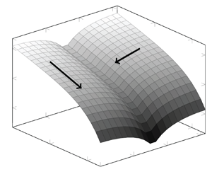
where $\varPi (k, z)$ and $\varPhi (k, z)$ are turbulent fluxes in wavenumber and physical space, respectively. Figure 1 depicts schematically these two fluxes in $(k,z)$ space. In the absence of inhomogeneity, the flux $\varPhi (k, z)$ is zero. In the inhomogeneous case, the presence of this flux will affect the kinetic energy spectrum $E(k, z)$.

Figure 1. A schematic of the energy spectrum in $(k,z)$ coordinates. Two arrows denote the directions of energy fluxes in wavenumber and physical space, respectively.

We model both fluxes using a gradient-diffusion approximation

(2.16)\begin{equation} \varPi(k, z) ={-}\rho(k, z)\,\frac{\partial (k^{{-}2}\,E(k, z))}{\partial k}, \end{equation}

with $\rho (k, z) \sim k^{11/2}\,E(k, z)^{1/2}$ being a turbulent energy diffusion in Fourier space, and

(2.17)\begin{equation} \varPhi(k, z) ={-}\mu(z)\,\frac{\partial E(k, z)}{\partial z}, \end{equation}

where $\mu (z)$ is a turbulent diffusivity in real space (see (2.29)). We have effectively decoupled (and simplified) the transfer terms in scale and physical space. Indeed, both $\varPhi (k, z)$ and $\varPi (k, z)$ are determined by the same triple velocity and velocity–pressure correlations (see (A4)). Decomposing the physical space–scale space flux is a major assumption that seems necessary to obtain an analytically tractable model of energy transfer in inhomogeneous turbulence. The model (2.16) for $\varPi (k, z)$ is known as the Leith model (Leith Reference Leith1967; Rubinstein & Clark Reference Rubinstein and Clark2022). This model tends to homogenise the kinetic energy in spectral space towards equipartition among wave vectors, corresponding to an energy spectrum proportional to $k^2$. The gradient-diffusion model for the diffusion (2.17) tends to homogenise the energy distribution in physical space, and is used in Besnard et al. (Reference Besnard, Harlow, Rauenzahn and Zemach1996), Touil, Bertoglio & Shao (Reference Touil, Bertoglio and Shao2002) and Cadiou, Hanjalić & Stawiarski (Reference Cadiou, Hanjalić and Stawiarski2004), for instance.

Eddy viscosity models are obviously simplified representations of the real transfer terms. For instance, see Pope (Reference Pope2000, § 10) for extensive discussion. However, we think that this kind of modelling is a useful first step before turning to more sophisticated modelling approaches.

2.4. Linear perturbation analysis and scaling predictions

Our goal is to derive a prediction for inertial range scaling at large Reynolds numbers in the limit of weak inhomogeneity, where the influence of inhomogeneity can be treated as a perturbation. In the following, the leading-order contributions and perturbations are indicated by subscripts $0$ and $1$, respectively. We define an inertial range $L^{-1} \ll k \ll \eta ^{-1}$, with the length $L$ representing the typical length of the largest and energy-containing scales of the flow. Furthermore, in our description, it is associated with the longest wavelength in our flow domain and is chosen constant. We will define this length scale more precisely later, in § 2.5.

We now define the equilibrium about which we expand the equations. To do so, we consider the decomposition

(2.18)\begin{equation} E(k, z) = E_0(k, z) + E_1(k, z), \end{equation}

with $|{E_1}| \ll |{E_0}|$. The other quantities, such as $\varPi (k, z)$ and $\varPhi (k, z)$, are decomposed in the same manner. We recall here that in addition to these two contributions to the energy spectrum, the flow also contains the time-averaged velocity profile, which consists of a single wave vector in the $z$-direction in the present case (see (2.2)). This mean flow is not present in the inertial range, on which we will focus in the following. Therefore, in the remainder of this section, we can focus on the contributions $E_0(k, z)$ and $E_1(k, z)$.

For very high Reynolds numbers in the limit of vanishing inhomogeneity, we assume that the equilibrium contributions to the kinetic energy balance (2.12) do not depend on the inhomogeneous turbulent diffusion $D(k, z)$. By integrating the balance between the transfer and dissipation terms in (2.12) from $k$ to $\infty$, we find

(2.19)\begin{equation} \int_k^\infty T(p, z) \,{\rm d}p = \int_k^\infty 2 \nu p^2 E(p, z) \,{\rm d}p \end{equation}

or, using (2.14) and the equilibrium/non-equilibrium decomposition,

(2.20)\begin{equation} \varPi_0(k, z) =\epsilon(z). \end{equation}

Indeed, this corresponds to the equilibrium between the energy flux and the energy dissipation rate, essential to the inertial range description of Kolmogorov (Reference Kolmogorov1941). The constant flux solution of the Leith model is consistent with this framework and is given by

(2.21)\begin{equation} E_0(k, z) \sim \epsilon(z)^{2/3}\,k^{{-}5/3}. \end{equation}

This expression defines our equilibrium solution. We now assess the influence of the inhomogeneity of $\epsilon (z)$ on this scaling as a perturbation.

In the following, we consider the terms in the balance equation (2.12) for the non-equilibrium contributions. The order of magnitude of the production term (2.13) and the diffusion-gradient modelling with the flux (2.17) lead us to deduce that $D(k, z)\gg P(k, z)$ at $k \gg L^{-1}$. Therefore, the first-order perturbation to the equilibrium scaling in the inertial range is due to the inhomogeneous diffusion $D(k, z)$. Then, in the inertial range, we have

(2.22)\begin{equation} T(k, z) ={-}D(k, z) \end{equation}

and

(2.23)\begin{equation} -\frac{\partial}{\partial k}\varPi_1(k, z) = \frac{\partial}{\partial z} \varPhi_0 (k, z), \end{equation}

since $\partial \varPi _0(k, z)/\partial k = 0$. Thus the first-order correction of the nonlinear transfer balances the zeroth-order contribution of the inhomogeneous diffusion. The first-order perturbation to the nonlinear flux $\varPi _1(k, z)$ is evaluated as (Rubinstein & Clark Reference Rubinstein and Clark2005)

(2.24)\begin{equation} \varPi_1(k, z) = E_1(k, z) \left.\frac{\partial\varPi}{\partial E}\right|_{E_0}, \end{equation}

where $\partial \varPi /\partial E|_{E_0}$ is the Fréchet derivative of the total flux $\varPi$ evaluated at $E(k, z) = E_0(k, z)$. In the inertial range, assuming $E_1$ to scale as a power law, this yields the scaling,

(2.25)\begin{equation} \varPi_1(k, z) \sim \epsilon(z)\,\frac{E_1(k, z)}{E_0(k, z)}. \end{equation}

Note that we obtain (2.25) not only for the Leith model, but also for most of the other classical closures, such as the Kovaznay and Heisenberg model (Rubinstein & Clark Reference Rubinstein and Clark2022). Integrating (2.23) from $k$ to $\infty$, we have

(2.26)\begin{equation} \varPi_1 (k, z) = \frac{\partial}{\partial z} \int_k^\infty \varPhi_0 (k, z) \,{\rm d}k. \end{equation}

By combining this with (2.17) and (2.25), we obtain

(2.27)\begin{equation} E_1 (k, z) \sim{-} \frac{E_0(k, z)}{\epsilon(z)}\,\frac{\partial}{\partial z} \left( \mu(z)\, \frac{\displaystyle\partial\int\nolimits_k^\infty E_0 (p, z) \,{\rm d}p}{\partial z} \right). \end{equation}

Substituting (2.21), the above expression gives

(2.28)\begin{equation} E_1(k, z) \sim{-}\mu(z)\,\epsilon(z)^{1/3}\,k^{{-}7/3} \left[ \frac23\,\frac{\epsilon_{zz}(z)}{\epsilon(z)} + \frac23\,\frac{\mu_z(z)}{\mu(z)}\,\frac{\epsilon_z(z)}{\epsilon(z)} - \frac29 \left(\frac{\epsilon_z(z)}{\epsilon(z)}\right)^2\right], \end{equation}

where the subscripts denote derivatives with respect to $z$, for example, $\epsilon _{zz} = \partial ^2 \epsilon (z) / \partial z^2$. We will model the unknown eddy diffusivity in its simplest way,

(2.29)\begin{equation} \mu(z) \sim L^{4/3}\,\epsilon(z)^{1/3}. \end{equation}

Doing so, we obtain

(2.30)\begin{equation} E_1(k, z) \sim{-}\frac{\epsilon_{zz}(z)\,L^{4/3}}{\epsilon(z)^{1/3}}\,k^{{-}7/3}. \end{equation}

Note that although all the terms involving $\epsilon _z$ and $\mu _z$ vanish exactly for the current definition of $\mu (z)$ in (2.29), this might not be the case for arbitrary choices of $\mu (z)$. It is therefore possible that in more sophisticated descriptions of turbulent diffusion, terms involving first-order derivatives might appear. In our description this is, however, not the case at leading order.

Considering expressions (2.25) and (2.30), it is observed that the non-equilibrium contribution $\varPi _1(k,z)$ to the energy flux flux can change sign, according to the sign of $\epsilon _{zz}(z)$. This implies that this part of the flux can vary from large to small $k$ values in the inertial range. However, since $\varPi _1$ is small compared to $\varPi _0$, the total flux in the inertial range, which is the sum of the two contributions, will be towards large $k$ as in the classical three-dimensional picture of an inertial range energy cascade.

2.5. Case of a sinusoidal dissipation profile

The comparison of (2.21) and (2.30) indicates that the inhomogeneous contribution ($\propto k^{-7/3}$) is subdominant compared to the equilibrium energy spectrum ($\propto k^{-5/3}$) at large wavenumbers. Furthermore, the expression is proportional to the second spatial derivative of the dissipation rate $\epsilon _{zz}(z)$ and can thus be both positive and negative. Let us illustrate the implication of this expression by considering a large-scale inhomogeneity characterised by a cosine function with a characteristic wavelength of order $L$:

(2.31)\begin{equation} \epsilon(z) = \langle{\epsilon}\rangle + \tilde{\epsilon} \cos(z/L), \end{equation}

with $\langle {\epsilon }\rangle \gg \tilde {\epsilon }$. We consider $L$, first introduced in § 2.4, to be of the order of and proportional to the characteristic large-scale length of the flow. Substituting this expression for $\epsilon (z)$ in (2.30), we find

(2.32)\begin{equation} E_1(k, z) = E_1^X(k)\cos(z/L), \end{equation}

with

(2.33)\begin{equation} E_1^X(k) = C_A \tilde{\epsilon} \langle{\epsilon}\rangle^{{-}1/3}L^{{-}2/3} k^{{-}7/3}, \end{equation}

where the superscript $X$ indicates the perturbations due to inhomogeneity.

Let us now assume that both the equilibrium spectrum $E_0(k, z)$ and $E_1(k, z)$ extend from $k=L^{-1}$ to $\infty$. Integrating the spectra in this range, we find that

(2.34)\begin{equation} K_0(z) \sim L^{2/3}\,\epsilon(z)^{2/3} \end{equation}

and

(2.35)\begin{equation} K_1(z) \sim{-}\frac{\epsilon_{zz}(z)\,L^2}{\langle{\epsilon}\rangle}\,K_0(z). \end{equation}

Comparing these last two expressions illustrates that the formal expansion parameter in our system is

(2.36)\begin{equation} \gamma = \frac{\epsilon_{zz}(z)\,L^2}{\langle{\epsilon}\rangle}. \end{equation}

The main analytical results of the present investigation, (2.33)–(2.35), are obtained by phenomenological modelling based on gradient-diffusion assumptions of nonlinear transfer in both physical and scale space. The models and their consequences are, at best, crude approximations of the intricate nonlinear interactions in the actual flow. Therefore, the resulting expressions need verification by experiments or DNS.

3. Assessment of the inhomogeneous scaling

3.1. Numerical set-up

In order to verify the theoretical predictions, in particular (2.33), we carry out DNS of three-dimensional Kolmogorov flow in a triple-periodic box. Such flow has the convenient properties of being statistically inhomogeneous in one direction and free of solid boundaries. Furthermore, its properties have been widely investigated numerically (Borue & Orszag Reference Borue and Orszag1996; Musacchio & Boffetta Reference Musacchio and Boffetta2014; Wu et al. Reference Wu, Schmitt, Calzavarini and Wang2021).

The dynamics of the Kolmogorov flow in the present investigation is governed by (2.1) with $f(z) = \sin (k_f z)$. The numerical domain is a cube of size $2{\rm \pi}$. These choices imply that the forcing wavelength is equal to the width of the cubic domain, and we set $k_f = L^{-1} = 1$. Simulations are carried out using a standard pseudo-spectral solver (Delache, Cambon & Godeferd Reference Delache, Cambon and Godeferd2014) with a third-order Adams–Bashforth time-integration scheme. The details of the simulations are reported in table 1. Since we focus on the effect of inhomogeneity, we attempt to obtain statistics in a steady state over a long-enough time interval to allow the effects of the temporal variations to become as small as possible (see the last column in table 1).

Table 1. DNS parameters and statistical quantities. The resolution $N$ and kinematic viscosity $\nu$ are the control parameters. The remaining statistical quantities are the fluctuating isotropic root mean square velocity $u' \equiv \sqrt {2K'/3}$, where the energy of the temporal fluctuating velocity is $K' \equiv \langle {u'_i u'_i}\rangle _{\boldsymbol {x}, t} / 2$ and $u'_i (\boldsymbol {x}, t) \equiv u_i (\boldsymbol {x}, t) - \langle {u_i}\rangle _t(\boldsymbol {x})$; the Taylor microscale $\lambda \equiv u' \sqrt {15 \nu / \epsilon }$, where the energy dissipation rate is evaluated by $\epsilon = \nu \langle {\omega _i \omega _i}\rangle _{\boldsymbol {x}, t}$; the Taylor-length Reynolds number $Re_\lambda \equiv u' \lambda / \nu$; the integral time scale $T \equiv L/u'$, with $L = k_f^{-1} = 1$; and the simulation time in the statistically steady state $T_{total}$ as a function of $T$.

3.2. Visualisation and dissipation profile

In the following, we will discuss the simulation at the highest considered Reynolds number $Re_\lambda =184$. A flow visualisation is shown in figure 2(a) with the $x$-component of the velocity field $\mathcal {U}_x (\boldsymbol {x}, t)$. The influence of the large-scale mean flow, proportional to the sinusoidal forcing along the $z$-axis, is distinguishable. Figure 2(b) shows the instantaneous profile of $\mathcal {U}_x (z, t) = \langle {\mathcal {U}_x (\boldsymbol {x}, t)}\rangle _{\perp }$. The single curve corresponds to the horizontal average of a snapshot, as shown in figure 2(a). Its time average $U(z) = \langle {\mathcal {U}_x (\boldsymbol {x}, t)}\rangle _{\perp, t}$ is also shown in figure 2(b) with a smooth sinusoidal profile.

Figure 2. (a) Instantaneous distributions of $\mathcal {U}_x(\boldsymbol {x}, t)$ at $Re_\lambda =184$. Blue (red) corresponds to the negative (positive) value of $\mathcal {U}_x$. (b) Instantaneous profiles of $\mathcal {U}_x(z, t) = \langle {\mathcal {U}_x(\boldsymbol {x}, t)}\rangle _{\perp }$ in grey. Time-averaged profile $U(z) = \langle {\mathcal {U}_x(\boldsymbol {x}, t)}\rangle _{\perp, t}$ is indicated by a thick line.

In figure 3(a), the instantaneous profile of the energy dissipation rate $\epsilon (z, t) = \langle {\epsilon (\boldsymbol {x}, t)}\rangle _{\perp }$ is shown along with its time average $\epsilon (z) = \langle {\epsilon (\boldsymbol {x}, t)}\rangle _{\perp, t}$. The instantaneous profile shows large fluctuations in comparison to the velocity profile (figure 2b). Its time average, in contrast, shows a smooth sinusoidal profile. This property allows us to use the approximations in § 2.5. As expected, the dissipation peaks at values where the mean velocity gradient is strongest (at $z = 0$ and $\pm {\rm \pi}$). For numerical convenience, we perform a sinusoidal fitting $\bar {\epsilon }(z)$ introduced in (2.31). This profile is also shown in figure 3(a).

Figure 3. (a) Instantaneous profile of $\epsilon (z, t) = \langle {\epsilon (\boldsymbol {x}, t)}\rangle _{\perp }$. The time-averaged profile $\epsilon (z) = \langle {\epsilon (\boldsymbol {x}, t)}\rangle _{\perp, t}$ is also shown. The red dashed line denotes $\bar {\epsilon }(z)$, a sinusoidal fitting of $\epsilon (z)$ by (2.31). (b) Time-averaged profile of kinetic energy with fluctuating velocity $K(z)$, and its equilibrium $K_0(z)$ and non-equilibrium $K_1(z)$ contributions. See the main text and Appendix B for the definition.

Figure 3(b) shows the kinetic energy profile of the fluctuating velocity field. The fluctuating energy profile is defined by $K(z, t) = \mathcal {K}(z, t) - K_U(z)$, where the total energy is $\mathcal {K}(z, t) = \mathcal {U}_i (z, t)\,\mathcal {U}_i (z, t) / 2$ and the mean flow energy is $K_U(z) = U(z)^2 / 2$. We consider the decomposition (see (2.34)–(2.35) and Appendix B)

(3.1)\begin{equation} K(z, t) = K_0(z, t) + K_1(z, t). \end{equation}

In figure 3(b), we observe that the equilibrium $K_0(z) = \langle {K_0(z, t)}\rangle _t$ and the non-equilibrium $K_1(z) = \langle {K_1(z, t)}\rangle _t$ profiles share the same phase, consistent with the prediction that the spectrum $E_1(k, z)$ is proportional to $-\partial ^2\epsilon (z)/\partial z^{2}$.

3.3. Equilibrium and non-equilibrium spectra

Figure 4 shows the isotropic energy spectrum $E(k, t)$ (see Appendix A for the definition) at three different Taylor-length Reynolds numbers. For simplicity, we denote its time average by $E(k) = \langle {E(k, t)}\rangle _t$. Normalisation using $\nu$ and $\epsilon = \langle {\epsilon (\boldsymbol {x}, t)}\rangle _{\boldsymbol {x}, t}$ allows an excellent collapse for large values of $k$.

Figure 4. Time-averaged three-dimensional isotropic energy spectrum $E(k) = \langle {E(k, t)}\rangle _t$, normalised by Kolmogorov variables. Results are shown at $Re_\lambda =69.6$, $113$ and $184$ (see table 1). The red dashed line denotes the $k^{-5/3}$ scaling for reference.

Next, we assess energy spectra in statistically homogeneous planes perpendicular to the $z$-axis, as defined in (2.9). In the following, we analyse the time-averaged inhomogeneous energy spectrum $E(k_\perp, z) = \langle {E(k_\perp, z, t)}\rangle _t$ in a statistically steady state (see table 1). Figure 5(a) shows $E(k_\perp, z)$ non-dimensionalised by $\bar {\epsilon }(z)^{2/3}\,L^{2/3}$. The fluctuations at small scales are small, and variations are barely visible.

Figure 5. (a) Non-dimensionalised two-dimensional energy spectrum. Note that $E(k_\perp, z) = \langle {E(k_\perp, z, t)}\rangle _t$. Dark (light) colour represents the small (large) value of the $z$-coordinate. The thick black line denotes (3.3), the average over the $z$-coordinate. (b) Time-averaged non-equilibrium energy spectrum with specific signs: $E_1^+ (k_\perp ) = \langle {E_1(k_\perp, z) > 0}\rangle _z$ and $E_1^- (k_\perp ) = \langle {E_1(k_\perp, t) < 0}\rangle _z$. Red dashed lines denote the $k_\perp ^{-7/3}$ slope.

Then we assume that the energy spectrum in the inertial range can be written, in a general form, as

(3.2)\begin{equation} E_0(k_\perp, z) \sim \epsilon(z)^{2/3}\,k_\perp^{{-}5/3}\,f_L[k_\perp L]\,f_\eta[k_\perp\,\eta(z)], \end{equation}

where $f_L$ and $f_\eta$ determine the shapes at small and large $k$, respectively. Therefore, there are two distinct choices to collapse the spectra. See Appendix B for the detail of the two normalisation procedures. In this study, we employ the large-scale normalisation and evaluate

(3.3)\begin{equation} f_L[k_\perp L] \equiv \left\langle{E(k_\perp, z)\,\bar{\epsilon}(z)^{{-}2/3}\,k_\perp^{5/3}}\right\rangle_z, \end{equation}

as shown in figure 5(a). Note that this expression is valid for $k_\perp \eta \ll 1$, where $f_\eta (k_\perp \eta )$ tends to a constant value. Then the equilibrium spectrum can be defined as

(3.4)\begin{equation} E_0 (k_\perp, z) \equiv \bar{\epsilon}(z)^{2/3}\,f_L[k_\perp L]\,k_\perp^{{-}5/3}. \end{equation}

Now we can evaluate the non-equilibrium spectrum by $E_1(k_\perp, z) \equiv E(k_\perp, z) - E_0(k_\perp, z)$. Note that (i) this quantity is defined by the time-averaged spectra, and (ii) since this quantity can be regarded as a perturbation of $E(k_\perp, z)$ around $E_0(k_\perp, z)$, it can be both positive and negative. Figure 5(b) shows the $z$-average of $E(k_\perp, z)$ for specific signs.

Similar plots are shown in figure 10 of Horiuti & Ozawa (Reference Horiuti and Ozawa2011) and figure 2 of Horiuti & Tamaki (Reference Horiuti and Tamaki2013). The scaling is consistent with that derived in § 2.4, i.e.

(3.5)\begin{equation} \langle{|{E_1(k_\perp, z)}|}\rangle_z \propto k_\perp^{{-}7/3}. \end{equation}

Figure 6(a) compares $\langle {|{E_1(k_\perp, z)}|}\rangle _z$ for three different Reynolds numbers, as in figure 4. For smaller values of $Re_\lambda$, the spectrum exhibits scaling steeper than $k_\perp ^{-7/3}$. At larger $Re_\lambda$, the slope approaches the $k_\perp ^{-7/3}$ scaling. At the same time, the spectrum in the higher $k_\perp$ range exhibits a bump associated with scaling shallower than $k_\perp ^{-7/3}$.

Figure 6. (a) Absolute value of the time-averaged non-equilibrium energy spectrum $|{E_1(k_\perp, z)}| = |{\langle {E_1(k_\perp, z, t)}\rangle _t}|$ for three values of the Taylor-length Reynolds numbers. The red dashed line represents the $k_\perp ^{-7/3}$ scaling. (b) Compensated spectrum of (a). The red dashed line denotes the compensated $k_\perp ^{-7/3}$ scaling.

We plot the compensated spectra in figure 6(b). Although the scaling range extends for less than a decade, the emergence of the $k_\perp ^{-7/3}$ scaling range is well captured using this normalisation. In Appendix B, we confirm that the bump in the compensated spectra is due to our choice of the non-dimensional function (3.2).

4. Conclusion and discussion

The numerical simulations in the previous section support our prediction,

(4.1)\begin{equation} E(k, z) = C_K\,\epsilon(z)^{2/3}\,k^{{-}5/3} - C_A\,\frac{\epsilon_{zz}(z)\,L^{4/3}}{\epsilon(z)^{1/3}}\, k^{{-}7/3}, \end{equation}

of the energy spectrum for turbulence with inhomogeneity in the $z$-direction. This scaling quantifies the influence of spatial inhomogeneity in wavenumber space. In particular, the special case where the dissipation fluctuates as a sinusoidal function around a mean value, discussed in § 2.5, gives us a useful estimate of the influence of inhomogeneity (see (2.32)–(2.33)). Indeed, introducing an average dissipation $\langle {\epsilon }\rangle$ and smooth spatial fluctuations $\tilde {\epsilon }$ around $\langle {\epsilon }\rangle$, so that $\epsilon _{zz}/\tilde {\epsilon }\sim L^{-2}$, we obtain

(4.2)\begin{equation} \frac{E^X_1(k, z)}{E_0(k, z)} \sim \frac{\tilde{\epsilon}}{\langle{\epsilon}\rangle}\,(kL)^{{-}2/3}. \end{equation}

This expression shows that the influence of large-scale inhomogeneity is negligible for

(4.3)\begin{equation} k \gg L^{{-}1}\left(\frac{\tilde{\epsilon}}{\langle{\epsilon}\rangle}\right)^{3/2}. \end{equation}

Therefore, if this requirement is fulfilled in a statistically stationary flow, far enough away from walls, then Kolmogorov's equilibrium spectrum is expected to be dominant compared to the contributions associated with spatial inhomogeneity.

Funding

We dedicate this work to J.-P. Bertoglio, on the occasion of his retirement. All DNS were carried out using the facilities of the PMCS2I (École Centrale de Lyon). R.A. is supported by the Takenaka Scholarship Foundation.

Declaration of interests

The authors report no conflict of interest.

Appendix A. Governing equation of the inhomogeneous energy spectrum

In this appendix, we define the spectrum and the governing equations for the energy spectrum tensor in inhomogeneous flow (see (2.12)). The generalised spectrum $E(k, \boldsymbol {x}) = E_{ii} (k, \boldsymbol {x})$ is defined by

(A1)\begin{equation} E(k, \boldsymbol{x}) \equiv \frac12 \iint {\rm e}^{-\mathrm{i} \boldsymbol{k} \boldsymbol{\cdot} \boldsymbol{r}} \left\langle{ u_i \left(\boldsymbol{x} + \frac{\boldsymbol{r}}{2}\right) u_i \left(\boldsymbol{x} - \frac{\boldsymbol{r}}{2}\right)}\right\rangle {\rm d}{\boldsymbol{r}} \,{\rm d}{\varOmega_k}, \end{equation}

where $\int {\rm d}{\varOmega _k}$ denotes the integral over spherical shells of radius $k$. The brackets in this appendix denote the ensemble average. For statistically homogeneous turbulence, this definition is equivalent to the expression

(A2)\begin{equation} E(k) \equiv \int \tfrac{1}{2}\langle{u_i (\boldsymbol{k})\,u_i^\ast (\boldsymbol{k})}\rangle \,{\rm d}{\varOmega_k}. \end{equation}

The evolution equation for $E_{ij} (k, \boldsymbol {x}, t)$ formally reads

(A3)\begin{equation} \frac{\partial E_{ij} (k, \boldsymbol{x}, t)}{\partial t} = \frac12 \int \left[ \int {\rm e}^{-\mathrm{i} \boldsymbol{k} \boldsymbol{\cdot} \boldsymbol{r}} \varPsi_{ij} (\boldsymbol{x} + \boldsymbol{r}/2, \boldsymbol{x} - \boldsymbol{r}/2, t) \,{\rm d}{\boldsymbol{r}} \right] {\rm d}{\varOmega_k}. \end{equation}

For the tensor on the right-hand side, we have

(A4) \begin{align} \varPsi_{ij} (\boldsymbol{x}_1, \boldsymbol{x}_2) &= \nu \left(\nabla^2_1 + \nabla^2_2\right) R_{ij} (\boldsymbol{x}_1, \boldsymbol{x}_2) \nonumber\\ &\quad - \left[\frac{\partial}{\partial x_{1n}} U_n (\boldsymbol{x}_1)\,R_{ij} (\boldsymbol{x}_1,\boldsymbol{x}_2) + \frac{\partial}{\partial x_{2n}} U_n (\boldsymbol{x}_2)\,R_{ij} (\boldsymbol{x}_1,\boldsymbol{x}_2)\right.\nonumber\\ &\quad + \left. \frac{\partial}{\partial x_{1n}} U_i (\boldsymbol{x}_1)\,R_{nj} (\boldsymbol{x}_1,\boldsymbol{x}_2) + \frac{\partial}{\partial x_{2n}} U_j (\boldsymbol{x}_2)\,R_{ni} (\boldsymbol{x}_1,\boldsymbol{x}_2)\right. \nonumber\\ &\quad + \left. \frac{\partial}{\partial x_{1i}} \langle{ \mathcal{P}(\boldsymbol{x}_1)\,u_j(\boldsymbol{x}_2) }\rangle + \frac{\partial}{\partial x_{2j}} \langle{ \mathcal{P}(\boldsymbol{x}_2)\,u_i(\boldsymbol{x}_1) }\rangle \right.\nonumber\\ &\quad + \left. \frac{\partial}{\partial x_{1n}} \langle{u_i(\boldsymbol{x}_1)\,u_n(\boldsymbol{x}_1)\,u_j(\boldsymbol{x}_2) }\rangle + \frac{\partial}{\partial x_{2n}} \langle{ u_j(\boldsymbol{x}_2)\,u_n(\boldsymbol{x}_2)\,u_i(\boldsymbol{x}_1) }\rangle\right]. \end{align}

In this expression and the following, the argument $t$ for time is omitted for visibility. The two-point velocity tensor is defined by

(A5)\begin{equation} R_{ij} (\boldsymbol{x}_1, \boldsymbol{x}_2) \equiv \langle{u_i (\boldsymbol{x}_1)\,u_j (\boldsymbol{x}_2)}\rangle, \end{equation}

and (A4) is completed by incompressibility conditions for the mean field and the fluctuations.

Both inhomogeneous turbulence diffusion and spectral transfer are associated with the last two lines of expression (A4). An assumption of weak inhomogeneity must be invoked to dissociate them to obtain a closed expression. Even retaining only the leading-order terms in an expansion about inhomogeneity, the resulting equations become quite cumbersome (see Laporta Reference Laporta1995; Besnard et al. Reference Besnard, Harlow, Rauenzahn and Zemach1996).

Subsequently, the different terms in (A4) need to be modelled to close the triple correlations. We will not proceed in this direction, and will model them directly by their physical effects. See (2.13)– (2.16).

Appendix B. Normalisation to extract the non-equilibrium spectrum and kinetic energy profile

In this appendix, we investigate the different normalisation procedures mentioned in § 3.3. We state that the energy spectrum is decomposed into equilibrium (labelled by the subscript $0$) and non-equilibrium (labelled by the subscript $1$) contributions as

(B1)\begin{equation} E(k, z) = E_0(k, z) + E_1(k, z). \end{equation}

We further assume that the non-equilibrium contributions are zero-mean:

(B2)\begin{equation} \langle{ E_1(k, z) }\rangle_z = 0. \end{equation}

We have therefore

(B3)\begin{equation} \langle{ E(k, z) }\rangle_z = \langle{ E_0(k, z) }\rangle_z. \end{equation}

In order to compute the non-equilibrium contributions $E_1(k, z) = E(k, z) - E_0(k, z)$, we need to know the $z$-dependence of $E_0(k, z)$. For this purpose, we use self-similarity assumptions and Kolmogorov's equilibrium hypothesis.

Scaling ranges in turbulence spectra appear when scale separation is attained, i.e. at sufficiently high Reynolds numbers. In general, one can write the energy spectrum to scale as (see (3.2))

(B4)\begin{equation} E_0(k, z) \sim \epsilon(z)^{2/3}\,k^{{-}5/3}\,f_L[kL]\,f_\eta[k\eta(z)], \end{equation}

at high Reynolds numbers. We have two non-dimensional functions in (B4): $f_L$ determines the shape of the spectrum for small $k$ (large scale), and $f_\eta$ determines it for large $k$ (small scale). These functions satisfy the framework of Kolmogorov (Reference Kolmogorov1941):

(B5)\begin{equation} \lim_{x\rightarrow 0} f_\eta[x] = \lim_{x\rightarrow \infty} f_L[x] = 1. \end{equation}

Therefore, we retrieve (1.1) for scales $L^{-1} \ll k \ll \eta ^{-1}$ in the limit $L/\eta \rightarrow \infty$. Multiplying both sides of (B4) by $\eta ^{-5/3}$, and dividing by $\epsilon ^{2/3}$, we obtain

(B6)\begin{equation} \frac{E_0(k, z)}{\epsilon(z)^{1/4}\,\nu^{5/4}} = F_\eta[k\,\eta(z)]\,f_L[kL], \end{equation}

with

(B7)\begin{equation} F_\eta[k\,\eta(z)] = (k\eta)^{{-}5/3}\,f_\eta[k\,\eta(z)]. \end{equation}

Since $F(kL)$ tends to unity for $k \gg 1/L$, the equilibrium spectra $E_0(k, z)$ should collapse when normalised by (B6) for any $z$, for large $kL$.

Similarly, if the large scales are characterised by a length scale $L$, then we can propose an alternative normalisation for (B6):

(B8)\begin{equation} \frac{E_0(k, z)}{\epsilon(z)^{2/3}\,L^{5/3}} \sim F_L[k L]\,f[k\eta], \end{equation}

with

(B9)\begin{equation} F_L[k L] = (kL)^{{-}5/3}\,f_L[k L]. \end{equation}

It should scale as purely a function of $kL$ for $k\eta \ll 1$.

There are therefore two normalisation possibilities. One focuses on the high wavenumber limit of the inertial range close to the dissipation range (B6)–(B7), and the other one on the low-$k$ range close to the energy range (B8)–(B9). In the limit of infinite Reynolds number, we should find them to be equivalent in the inertial range, since

(B10)\begin{equation} \lim_{x\to\infty} F_L[x] = \lim_{x\to 0} F_\eta[x] = x^{{-}5/3}. \end{equation}

Figure 7 plots the absolute value of the non-equilibrium energy spectrum $E_1(k_\perp, z)$ for these two normalisations. It is observed that using $F[kL]$, we reveal a larger inertial range. We will therefore use this normalisation in the present investigation.

Figure 7. Absolute value of the time-averaged non-equilibrium energy spectrum $|{E_1(k_\perp, z)}| = |{\langle {E_1(k_\perp, z, t)}\rangle _t}|$ for the highest Reynolds number dataset. Different non-dimensionalised functions are employed to compute the non-equilibrium spectrum: (a) with (B7), and (b) with (B9). The black solid and red dashed lines denote the $z$-average and $k_\perp ^{-7/3}$ scaling, respectively.

We have checked the data, and we verified that the spectra $E_1(k_\perp,z)$ are for a given $z$ of a single sign, with a very occasional sign change when the statistics are determined over a too short time interval. Perturbation spectra are, as predicted, proportional to $-\epsilon _{zz}(z)$, as is also the case for $K_1(z)$, as can be seen by comparing figures 3(a) and 3(b). The procedure to determine $K_1(z)$ is now outlined.

Since the kinetic energy is determined dominantly by large scales, (B8) allows us to determine the equilibrium kinetic energy profile:

(B11)\begin{equation} K_0(z) = \int E_0(k, z) \,{\rm d}k = C_L\,\epsilon(z)^{2/3}\,L^{2/3}, \end{equation}

with $C_L = \int F_L [x] \,{\rm d}\kern0.06em x$. Then we define the decomposition

(B12)\begin{equation} K_0(z) = \langle{K(z)}\rangle_z + \tilde{K}_0(z), \end{equation}

where $\langle {K_0 (z)}\rangle _z = \langle {K(z)}\rangle _z$ follows from the assumption that $\langle {K_1(z)}\rangle _z = 0$. By employing the decomposition for the energy dissipation rate profile

(B13)\begin{equation} \epsilon(z)^{2/3} = \left\langle{\epsilon(z)^{2/3}}\right\rangle_z + \widetilde{\epsilon(z)^{2/3}}, \end{equation}

it follows from (B11) that

(B14)\begin{equation} \frac{\tilde{K}_0(z)}{\langle{K_0(z)}\rangle_z} = \frac{\widetilde{\epsilon(z)^{2/3}}}{\langle{\epsilon(z)^{2/3}}\rangle_z}, \end{equation}

and by (B12),

(B15)\begin{equation} K_0(z) = \left(1 + \frac{\widetilde{\epsilon(z)^{2/3}}}{\langle{\epsilon(z)^{2/3}}\rangle_z}\right) \langle{K(z)}\rangle_z. \end{equation}

Since all the terms on the right-hand side are known, one can evaluate the non-equilibrium kinetic energy profile $K_1(z) = K(z) - K_0(z)$ (see (3.1)).

References

Bertoglio, J.-P., Bataille, F. & Marion, J.-D. 2001 Two-point closures for weakly compressible turbulence. Phys. Fluids 13 (1), 290310.CrossRefGoogle Scholar
Bertoglio, J.-P. & Jeandel, D. 1987 A simplified spectral closure for inhomogeneous turbulence: application to the boundary layer. In Turbulent Shear Flows 5: Selected Papers from the Fifth International Symposium on Turbulent Shear Flows, Cornell University, Ithaca, New York, August 7–9 1985 (ed. F. Durst, B.E. Launder, J.L. Lumley, F.W. Schmidt & J.H. Whitelaw), pp. 19–30. Springer.CrossRefGoogle Scholar
Besnard, D.C., Harlow, F.H., Rauenzahn, R.M. & Zemach, C. 1996 Spectral transport model for turbulence. Theor. Comput. Fluid Dyn. 8 (1), 135.CrossRefGoogle Scholar
Borue, V. & Orszag, S.A. 1996 Numerical study of three-dimensional Kolmogorov flow at high Reynolds numbers. J. Fluid Mech. 306, 293323.CrossRefGoogle Scholar
Bos, W.J.T. 2020 Production and dissipation of kinetic energy in grid turbulence. Phys. Rev. Fluids 5 (10), 104607.CrossRefGoogle Scholar
Bos, W.J.T. & Rubinstein, R. 2017 Dissipation in unsteady turbulence. Phys. Rev. Fluids 2 (2), 022601.CrossRefGoogle Scholar
Briard, A., Gréa, B.-J., Mons, V., Cambon, C., Gomez, T. & Sagaut, P. 2018 Advanced spectral anisotropic modelling for shear flows. J. Turbul. 19 (7), 570599.CrossRefGoogle Scholar
Cadiou, A., Hanjalić, K. & Stawiarski, K. 2004 A two-scale second-moment turbulence closure based on weighted spectrum integration. Theor. Comput. Fluid Dyn. 18 (1), 126.CrossRefGoogle Scholar
Cambon, C., Jeandel, D. & Mathieu, J. 1981 Spectral modelling of homogeneous non-isotropic turbulence. J. Fluid Mech. 104, 247262.CrossRefGoogle Scholar
Delache, A., Cambon, C. & Godeferd, F. 2014 Scale by scale anisotropy in freely decaying rotating turbulence. Phys. Fluids 26 (2), 025104.CrossRefGoogle Scholar
Horiuti, K. & Ozawa, T. 2011 Multimode stretched spiral vortex and nonequilibrium energy spectrum in homogeneous shear flow turbulence. Phys. Fluids 23 (3), 035107.CrossRefGoogle Scholar
Horiuti, K. & Tamaki, T. 2013 Nonequilibrium energy spectrum in the subgrid-scale one-equation model in large-eddy simulation. Phys. Fluids 25 (12), 125104.CrossRefGoogle Scholar
Ishihara, T., Yoshida, K. & Kaneda, Y. 2002 Anisotropic velocity correlation spectrum at small scales in a homogeneous turbulent shear flow. Phys. Rev. Lett. 88 (15), 154501.CrossRefGoogle Scholar
Jeandel, D., Brison, J.F. & Mathieu, J. 1978 Modeling methods in physical and spectral space. Phys. Fluids 21 (2), 169182.CrossRefGoogle Scholar
Kaneda, Y. & Yoshida, K. 2004 Small-scale anisotropy in stably stratified turbulence. New J. Phys. 6 (1), 34.CrossRefGoogle Scholar
Knight, B. & Sirovich, L. 1990 Kolmogorov inertial range for inhomogeneous turbulent flows. Phys. Rev. Lett. 65 (11), 1356.CrossRefGoogle ScholarPubMed
Kolmogorov, A.N. 1941 The local structure of turbulence in incompressible viscous fluid for very large Reynolds numbers. Dokl. Akad. Nauk SSSR 30, 299303.Google Scholar
Kraichnan, R.H. 1971 An almost-Markovian Galilean-invariant turbulence model. J. Fluid Mech. 47 (3), 513524.CrossRefGoogle Scholar
Kurien, S., L'vov, V.S., Procaccia, I. & Sreenivasan, K.R. 2000 Scaling structure of the velocity statistics in atmospheric boundary layers. Phys. Rev. E 61 (1), 407.CrossRefGoogle ScholarPubMed
Laporta, A. 1995 Etude spectrale et modélisation de la turbulence inhomogène. PhD thesis, Ecole Centrale de Lyon.Google Scholar
Laporta, A. & Bertoglio, J.-P. 1995 A model for inhomogeneous turbulence based on two-point correlations. In Advances in Turbulence V: Proceedings of the Fifth European Turbulence Conference, Siena, Italy, 5–8 July 1994 (ed. R. Benzi), pp. 286–297. Springer.CrossRefGoogle Scholar
Leith, C.E. 1967 Diffusion approximation to inertial energy transfer in isotropic turbulence. Phys. Fluids 10 (7), 14091416.CrossRefGoogle Scholar
Liao, Z.-J. & Su, W.-D. 2015 Kolmogorov's hypotheses and global energy spectrum of turbulence. Phys. Fluids 27 (4), 041701.CrossRefGoogle Scholar
Moser, R.D. 1994 Kolmogorov inertial range spectra for inhomogeneous turbulence. Phys. Fluids 6 (2), 794801.CrossRefGoogle Scholar
Musacchio, S. & Boffetta, G. 2014 Turbulent channel without boundaries: the periodic Kolmogorov flow. Phys. Rev. E 89 (2), 023004.CrossRefGoogle ScholarPubMed
Parpais, S. & Bertoglio, J.-P. 1996 A spectral closure for inhomogeneous turbulence applied to turbulent confined flow. In Advances in Turbulence VI: Proceedings of the Sixth European Turbulence Conference, held in Lausanne, Switzerland, 2–5 July 1996 (ed. S. Gavrilakis, L. Machiels & P.A. Monkewitz), pp. 75–76. Springer.CrossRefGoogle Scholar
Pope, S.B. 2000 Turbulent Flows. Cambridge University Press.CrossRefGoogle Scholar
Rubinstein, R. & Clark, T. 2022 Reassessment of the Classical Turbulence Closures. Cambridge Scholars Publishing.Google Scholar
Rubinstein, R. & Clark, T.T. 2005 Self-similar turbulence evolution and the dissipation rate transport equation. Phys. Fluids 17 (9), 095104.CrossRefGoogle Scholar
Tennekes, H. & Lumley, J.L. 1972 A First Course in Turbulence. MIT.CrossRefGoogle Scholar
Touil, H., Bertoglio, J.-P. & Shao, L. 2002 The decay of turbulence in a bounded domain. J. Turbul. 3 (1), 049.CrossRefGoogle Scholar
Woodruff, S.L. & Rubinstein, R. 2006 Multiple-scale perturbation analysis of slowly evolving turbulence. J. Fluid Mech. 565, 95103.CrossRefGoogle Scholar
Wu, W., Schmitt, F.G., Calzavarini, E. & Wang, L. 2021 A quadratic Reynolds stress development for the turbulent Kolmogorov flow. Phys. Fluids 33 (12), 125129.CrossRefGoogle Scholar
Yoshizawa, A. 1984 Statistical analysis of the deviation of the Reynolds stress from its eddy-viscosity representation. Phys. Fluids 27 (6), 13771387.CrossRefGoogle Scholar
Yoshizawa, A. 1994 Nonequilibrium effect of the turbulent-energy-production process on the inertial-range energy spectrum. Phys. Rev. E 49 (5), 4065.CrossRefGoogle ScholarPubMed
Figure 0

Figure 1. A schematic of the energy spectrum in $(k,z)$ coordinates. Two arrows denote the directions of energy fluxes in wavenumber and physical space, respectively.

Figure 1

Table 1. DNS parameters and statistical quantities. The resolution $N$ and kinematic viscosity $\nu$ are the control parameters. The remaining statistical quantities are the fluctuating isotropic root mean square velocity $u' \equiv \sqrt {2K'/3}$, where the energy of the temporal fluctuating velocity is $K' \equiv \langle {u'_i u'_i}\rangle _{\boldsymbol {x}, t} / 2$ and $u'_i (\boldsymbol {x}, t) \equiv u_i (\boldsymbol {x}, t) - \langle {u_i}\rangle _t(\boldsymbol {x})$; the Taylor microscale $\lambda \equiv u' \sqrt {15 \nu / \epsilon }$, where the energy dissipation rate is evaluated by $\epsilon = \nu \langle {\omega _i \omega _i}\rangle _{\boldsymbol {x}, t}$; the Taylor-length Reynolds number $Re_\lambda \equiv u' \lambda / \nu$; the integral time scale $T \equiv L/u'$, with $L = k_f^{-1} = 1$; and the simulation time in the statistically steady state $T_{total}$ as a function of $T$.

Figure 2

Figure 2. (a) Instantaneous distributions of $\mathcal {U}_x(\boldsymbol {x}, t)$ at $Re_\lambda =184$. Blue (red) corresponds to the negative (positive) value of $\mathcal {U}_x$. (b) Instantaneous profiles of $\mathcal {U}_x(z, t) = \langle {\mathcal {U}_x(\boldsymbol {x}, t)}\rangle _{\perp }$ in grey. Time-averaged profile $U(z) = \langle {\mathcal {U}_x(\boldsymbol {x}, t)}\rangle _{\perp, t}$ is indicated by a thick line.

Figure 3

Figure 3. (a) Instantaneous profile of $\epsilon (z, t) = \langle {\epsilon (\boldsymbol {x}, t)}\rangle _{\perp }$. The time-averaged profile $\epsilon (z) = \langle {\epsilon (\boldsymbol {x}, t)}\rangle _{\perp, t}$ is also shown. The red dashed line denotes $\bar {\epsilon }(z)$, a sinusoidal fitting of $\epsilon (z)$ by (2.31). (b) Time-averaged profile of kinetic energy with fluctuating velocity $K(z)$, and its equilibrium $K_0(z)$ and non-equilibrium $K_1(z)$ contributions. See the main text and Appendix B for the definition.

Figure 4

Figure 4. Time-averaged three-dimensional isotropic energy spectrum $E(k) = \langle {E(k, t)}\rangle _t$, normalised by Kolmogorov variables. Results are shown at $Re_\lambda =69.6$, $113$ and $184$ (see table 1). The red dashed line denotes the $k^{-5/3}$ scaling for reference.

Figure 5

Figure 5. (a) Non-dimensionalised two-dimensional energy spectrum. Note that $E(k_\perp, z) = \langle {E(k_\perp, z, t)}\rangle _t$. Dark (light) colour represents the small (large) value of the $z$-coordinate. The thick black line denotes (3.3), the average over the $z$-coordinate. (b) Time-averaged non-equilibrium energy spectrum with specific signs: $E_1^+ (k_\perp ) = \langle {E_1(k_\perp, z) > 0}\rangle _z$ and $E_1^- (k_\perp ) = \langle {E_1(k_\perp, t) < 0}\rangle _z$. Red dashed lines denote the $k_\perp ^{-7/3}$ slope.

Figure 6

Figure 6. (a) Absolute value of the time-averaged non-equilibrium energy spectrum $|{E_1(k_\perp, z)}| = |{\langle {E_1(k_\perp, z, t)}\rangle _t}|$ for three values of the Taylor-length Reynolds numbers. The red dashed line represents the $k_\perp ^{-7/3}$ scaling. (b) Compensated spectrum of (a). The red dashed line denotes the compensated $k_\perp ^{-7/3}$ scaling.

Figure 7

Figure 7. Absolute value of the time-averaged non-equilibrium energy spectrum $|{E_1(k_\perp, z)}| = |{\langle {E_1(k_\perp, z, t)}\rangle _t}|$ for the highest Reynolds number dataset. Different non-dimensionalised functions are employed to compute the non-equilibrium spectrum: (a) with (B7), and (b) with (B9). The black solid and red dashed lines denote the $z$-average and $k_\perp ^{-7/3}$ scaling, respectively.