A generalized wall-pressure spectral model for non-equilibrium boundary layers

Abstract

This study uses high-fidelity simulations (direct numerical simulation or large-eddy simulation) and experimental datasets to analyse the effect of non-equilibrium streamwise mean pressure gradients (adverse or favourable), including attached and separated flows, on the statistics of boundary-layer wall-pressure fluctuations. The datasets collected span a wide range of Reynolds numbers ($Re_\theta$ from 300 to 23 400) and pressure gradients (Clauser parameter from $-0.5$ to 200). The datasets are used to identify an optimal set of variables to scale the wall-pressure spectrum: edge velocity, boundary layer thickness and the peak magnitude of Reynolds shear stress. Using the present datasets, existing semi-empirical models of the wall-pressure spectrum are shown unable to capture effects of strong, non-equilibrium adverse pressure gradients, due to inappropriate scaling of the wall pressure using the wall shear stress, calibration with limited types of flows and dependency on model parameters based on the friction velocity, which reduces to zero at the detachment point. To address these shortcomings, a generalized wall-pressure spectral model is developed with parameters that characterize the extent of the logarithmic layer and the strength of the wake. Derived from the local mean streamwise velocity profile, these two parameters inherently carry the effect of the Reynolds number, as well as those of the non-equilibrium pressure gradient and its history. Comparison with existing models shows that the proposed model behaves well and is more accurate in strong-pressure-gradient flows and in separated-flow regions.

1. Introduction

The fluctuation in space and time of the wall pressure beneath a turbulent boundary layer is one of the major sources of flow-induced noise and vibrations. Accurate modelling of the statistics of wall-pressure fluctuations is important for noise prediction in a wide range of applications such as wind turbines (Avallone et al. 2018; Deshmukh et al. 2019; Venkatraman et al. 2023), cooling fans (Sanjosé & Moreau 2018; Luo, Chu & Zhang 2020; Swanepoel, Biedermann & van der Spuy 2023), propellers (Casalino et al. 2021; Lallier-Daniels et al. 2021), unmanned/manned air vehicles or drones (Celik et al. 2021; Lauzon et al. 2023; Pargal, Li & Li 2023) and cabin noise (Samarasinghe, Zhang & Abhayapala 2016; Borelli et al. 2021), etc. as well as for prediction of flow-induced structure fatigue (Franco et al. 2020). In these applications, the boundary-layer flows are often turbulent and non-equilibrium, due to surface curvature and significant pressure gradients that vary in the streamwise direction, which may induce boundary-layer separation and can be found in a large range of Reynolds number. Here, a non-equilibrium boundary layer is defined as a boundary layer with streamwise (i.e. $x$) variation of the Clauser parameter, $\beta (x)=(\delta ^*/\tau _w)({\rm d}p_e/{{\rm d}{\kern0.8pt}x})$, where $\delta ^*(x)$ is the displacement thickness, $\tau _w(x)$ is the wall shear stress and $p_e(x)$ is the static pressure at the edge of the boundary layer. Therefore, the generation of noise in non-equilibrium turbulent boundary layers is physically complex and challenging to model.

The modelling of wall-pressure loading as a noise source predominantly depends on the power spectral density (PSD) of wall-pressure fluctuations, as well as its spanwise correlation length and the convection velocity of turbulent structures (Amiet 1976; Roger & Moreau 2005; Moreau & Roger 2009; Lee et al. 2021). The focus here is on modelling the wall-pressure spectrum (WPS). It is established that the WPS of a boundary layer with zero or minimal pressure gradient consists of three ranges (Farabee & Casarella 1991; Chang, Piomelli & Blake 1999; Goody 2004): (i) a range with $\omega ^2$ variation at low frequencies (where $\omega$ is the frequency), (ii) a range with $\omega ^{-5}$ behaviour at high frequencies and (iii) an overlap range with an approximate $\omega ^{-1}$ decay between the above two ranges. Based on data primarily in equilibrium flows, the width of the overlap range was found to increase with Reynolds number (Farabee & Casarella 1991; Goody 2004).

Contributions from different layers of wall turbulence to the WPS have been studied and are summarized below. The experimental studies of Farabee & Casarella (1991) suggested different dominant sources for different wavenumber ranges of the WPS: the high-wavenumber range is mainly attributed to turbulent activities in the logarithmic region, while the low-wavenumber range is attributed to large-scale turbulent motions in the outer layer. Van Blitterswyk & Rocha (2017) quantified the correlations between the fluctuations of wall pressure and those of streamwise velocity in different layers of the boundary layer and observed that high-frequency and overlap ranges of the WPS are associated with flows in the buffer and logarithmic regions, respectively. As opposed to earlier studies performed on channel flow or canonical flat-plate boundary-layer data, Jaiswal et al. (2020) analysed data collected near the trailing edge of a cambered aerofoil with a strong mean adverse pressure gradient (APG) in a highly non-equilibrium turbulent boundary layer, to compare contributions from various velocity sources (i.e. the mean-shear and turbulence–turbulence terms) at different wall-normal locations with the wall-pressure fluctuations based on the pressure Poisson's equation. They found that the mean-shear term in the inner and logarithmic regions is the dominant contributor, especially in the mid-to-high-frequency range.

Past studies were mostly on zero-pressure-gradient (ZPG) turbulent boundary layers. They showed that the wall-pressure fluctuations (evaluated by the root-mean-square values, $p_{rms}$) are amplified under a higher Reynolds number, mainly due to the increase in overlap-range spectral contribution. For a ZPG flat-plate boundary layer, Farabee & Casarella (1991) integrated the pressure spectrum over various frequency ranges and showed that the low-to-mid-frequency range and the high-frequency range were not sensitive to a change in Reynolds number, whereas the significance of the overlap range increases with Reynolds number, leading to an augmentation of $p_{rms}$. They proposed that $p_{rms}^2/\tau _w^2=6.5+1.86 \ln (Re_{\tau }/333)$, which was tested with ZPG boundary layer and channel flow data. Panton & Linebarger (1974) also demonstrated that the overlap range is correlated with the Reynolds number.

The current understanding of the WPS in non-zero-pressure-gradient flows is summarized as follows. Reviews of the earlier work before the mid-1990s are provided by Willmarth (1975) and Bull (1996). Schloemer (1967) showed that, under an APG, low-frequency contents of the WPS become more prominent as large eddies are energized, while the high-frequency contents become less important. Under a favourable pressure gradient (FPG), however, the opposite applies, with stronger high-frequency contents. The WPS slope in the overlap range also varies with the pressure gradient. Cohen & Gloerfelt (2018) investigated the effects of a mild pressure gradient using large-eddy simulations (LES) and showed scale-based dependencies of the WPS on FPG similar to those observed before. Na & Moin (1998) conducted direct numerical simulation (DNS) of a boundary layer with prescribed free-stream suction and blowing to induce flow separation and reattachment. They showed that none of the outer, inner or mixed scaling collapsed the wall-pressure spectra in all regions of the flow. Normalization with the local maximum magnitude of the Reynolds shear stress, however, was shown to collapse the low-frequency range of WPS for APG flows, including those with separation (Ji & Wang 2012; Abe 2017; Caiazzo et al. 2023).

Modelling of turbulent WPS is broadly classified in two categories: (i) semi-empirical modelling and (ii) analytical modelling based on solution of the Poisson equation of pressure (Kraichnan 1956; Panton & Linebarger 1974; Jaiswal et al. 2020; Grasso, Roger & Moreau 2022; Hales & Ayton 2023; Palani et al. 2023). The focus of this paper is on the first approach, which requires a smaller number of inputs from the flow field in comparison with the analytical modelling approach. Existing semi-empirical WPS closures mostly model the magnitude and shape of the WPS normalized by some boundary-layer parameters that are either internal, external or mixed, such as the boundary-layer thickness ($\delta$), the edge velocity ($U_e$) and the wall shear stress ($\tau _w=\rho u_\tau ^2$, where $u_{\tau }$ is the friction velocity and $\rho$ is the density), etc. For some of these studies see Kraichnan (1956), Corcos (1964), Willmarth (1975), Amiet (1976), Bull & Thomas (1976), Chase (1980), Goody (2004), Rozenberg, Robert & Moreau (2012), Kamruzzaman et al. (2015), Lee (2018), Hu (2018) and Pargal et al. (2022). Goody (2004) proposed a model for ZPG boundary layers, which accurately models the Reynolds-number effect on the WPS for these flows. To capture the pressure-gradient effect, several other models have been proposed (Rozenberg et al. 2012; Hu et al. 2013; Kamruzzaman et al. 2015; Catlett et al. 2016; Lee 2018; Rossi & Sagaut 2023). Rozenberg et al. (2012) integrated additional boundary-layer flow parameters to sensitize the model to pressure-gradient effects, especially those of APG. The additional parameters include Clauser's parameter ($\beta$) (Clauser 1954) and Cole's wake parameter ($\varPi$) (Coles 1956). The former includes the local effect of mean pressure gradients, while the latter represents the cumulative effect of the history of the mean pressure gradient up to the considered location in the boundary layer. Several later models developed modifications of the model that capture effects of other complexities such as wall curvature and FPG. Kamruzzaman et al. (2015) developed a model by fitting it on a large amount of experimental WPS data collected in various non-equilibrium boundary-layer flows on aerofoils. Hu (2018) used the shape factor ($H$) and Reynolds numbers ($Re_{\theta }$ or $Re_\tau$) instead of $\beta$ to incorporate the effect of non-equilibrium pressure gradients, as $\beta$ – a descriptor of the local pressure gradient – does not carry the history effect of a spatially varying pressure gradient. Lee (2018) improved Rozenberg's model based on experimental data gathered from a wide range of flows with different Reynolds numbers and pressure gradients. Thomson & Rocha (2022) proposed a new model for flows with FPG. Recently, machine learning approaches such as gene expression programming and artificial neural networks were used to model WPS as a function of boundary-layer parameters (Dominique et al. 2022; Fritsch et al. 2022a; Ghiglino et al. 2023; Shubham et al. 2023).

Despite the success of the models mentioned above in the specific flows for which they were developed, these models are not universally applicable to both ZPG flows and those with non-equilibrium pressure gradients and/or surface curvature, due to the following reasons. (i) Models developed by curve fitting to data of a limited type of flows do not naturally apply to other flows, such as Goody's model, which works for ZPG flows only. (ii) Normalizations of wall-pressure statistics used for ZPG flows (e.g. $\tau _w$) may not be appropriate for strong APG flows (e.g. a boundary layer close to separation where $\tau _w$ approaches zero). (iii) The choices of local boundary-layer parameters do not account sufficiently for the history effect of the pressure gradient. In addition, some existing models were developed based on experimental wall-pressure measurements that are supplemented with low-fidelity flow-field data, such as those estimated from XFOIL (Drela 1989).

The objective of this study is therefore to develop a general WPS model that is tuneable for both ZPG and non-equilibrium, strong-pressure-gradient turbulent boundary layers, as well as special cases such as flow separation and reattachment. To this end, model parameters that capture the local characteristics of the mean streamwise velocity profile (which evolves under a history of the pressure-gradient variation) are derived and incorporated to sensitize the model to the streamwise pressure gradient and its history. An appropriate pressure normalization for flows with and without pressure gradients is used. The model is calibrated based on a large and inclusive database, containing both experimental measurements and DNS/LES data (existing or new) of flows over a wide range of Reynolds number, with or without separation.

The organization of the paper is as follows. Section 2 describes the database, § 3 presents the boundary-layer development of the cases in the datasets, § 4 discusses the wall-pressure fluctuations and WPS in the datasets, § 5 discusses the performances of existing WPS models and then introduces a new generalized WPS model and conclusions are presented in § 6.

2. Dataset collection

The first step to develop a generalized WPS model is to collect and analyse high-fidelity datasets in a wide range of flows. The goal is to collect datasets for both equilibrium and non-equilibrium boundary layers, including ZPG, FPG and APG flows, with or without wall curvature (as in boundary layers developed on aerofoils) and boundary-layer separation and reattachment, across a wide range of Reynolds number based on momentum thickness ($Re_{\theta }=300$ to 23 400).

2.1. Simulation datasets

The DNS and LES datasets are gathered or re-generated from cases in four prior studies: Pargal et al. (2022), Wu et al. (2019), Na & Moin (1998) and Wu & Piomelli (2018). Details of the flows in these datasets are listed in table 1. The first three are DNS while Wu & Piomelli (2018) is a LES study. The data of Pargal et al. (2022) and Wu et al. (2019) are collected directly from simulations of a turbulent boundary layer on a flat plate and that on a controlled-diffusion (CD) aerofoil with matched non-equilibrium APG distributions along the streamwise direction. Comparison between these two flows reveal the effects of the convex wall curvature and the trailing edge on WPS, which were partially discussed in Pargal et al. (2022) and will be further discussed for the WPS herein. Na & Moin (1998) and Wu & Piomelli (2018) conducted simulations of flat-plate boundary layers with suction and blowing free-stream velocities, leading to boundary-layer separation and then reattachment; these two cases are rerun to collect boundary-layer parameters, streamwise mean velocity and wall-pressure statistics at the same streamwise locations, as these data were not fully available from the original publications. For the case of Wu & Piomelli (2018), this work provides new data as the wall pressure was not discussed previously.

Table 1. List of simulation datasets. For the cases of Na & Moin (1998) and Wu & Piomelli (2018), the boundary-layer separation leads to $\beta$ values between $-\infty$ and $\infty$. The Reynolds-number values are slightly different from those in Na & Moin (1998) and Wu & Piomelli (2018) due to difference in the definitions of the boundary-layer edge.

A brief summary of the four simulations is as follows. The case of Wu et al. (2019) provides DNS data on a boundary layer developing on the pressure side of a CD aerofoil, at a free-stream Mach number of 0.25. The compressible Navier–Stokes equations are solved for the flow around an aerofoil with the multi-block structured code HiPSTAR (High Performance Solver for Turbulence and Aeroacoustics Research) (Sandberg 2015). An initial two-dimensional Reynolds-averaged Navier–Stokes (RANS) simulation was run to provide boundary and initial conditions to the DNS simulation. Details of the problem formulation are provided by Wu et al. (2019). The simulation was validated against experimental data (Jaiswal 2020; Jaiswal et al. 2020) for wall-pressure spectral data and flow statistics at different streamwise locations. The case of Pargal et al. (2022) is an incompressible DNS of a flat-plate turbulent boundary layer to emulate the boundary-layer development on the downstream portion of the CD aerofoil flow studied by Wu et al. (2019). A finite difference solver on a staggered grid was used. To match the pressure-gradient parameter ($K$) of the aerofoil boundary layer, a streamwise pressure gradient was imposed by prescribing a streamwise-varying $U_\infty (x)$ at the top boundary of the domain. A fully turbulent boundary-layer flow at the inlet of the domain was obtained using the recycling/rescaling method. A convective outflow boundary condition was used at the outlet and periodic boundary conditions were used in the spanwise direction. Similar discretization methods and boundary conditions were used in Wu & Piomelli (2018) and Na & Moin (1998) with slight variations in details. Simulations of the flows in these two studies were rerun, based on the methodologies of Pargal et al. (2022). The meshes in the new simulations were similar to those in the original studies. The same domain lengths and similar boundary conditions were used. The rerun simulation of Na & Moin (1998) has been validated against results reported in the original work on flow statistics and wall-pressure spectra at different streamwise locations. For the rerun LES simulation of Wu & Piomelli (2018), the governing equations were solved for the filtered velocities at scales larger than the low-pass filter. A different dynamic eddy-viscosity model based on the Lagrangian-averaging procedure (Meneveau, Lund & Cabot 1996) was used for the present simulation. Boundary-layer developments in the rerun simulations will be compared with those reported in the original studies in § 3.

2.2. Experimental datasets

The DNS and LES simulations are limited to comparatively low Reynolds numbers $(Re_{\theta }=300$ to 7000). Experimental datasets are gathered from the studies of Hu (2018), Fritsch et al. (2022b) and Goody & Simpson (2000), which provide ZPG or pressure-gradient flow data with $Re_\theta$ of up to 23 400. Only existing datasets with both mean velocity profile data and WPS data measured at the same streamwise locations are included, as these quantities are required to calibrate and test the proposed model to be introduced in § 5.2.

A brief description of the experimental set-up of each case is given below. Hu (2018) carried out experiments in an open-jet anechoic test section of the Acoustic Wind Tunnel Braunschweig (AWB). Adverse and favourable pressure gradients in flat-plate boundary layers were achieved by placing a rotatable NACA 0012 aerofoil above the flat plate. Wall-pressure statistics were measured with sub-miniature pressure transducers and boundary-layer velocity profiles were obtained using hot-wires. The value of $Re_{\theta }$ was up to 19,000, with $\beta =-0.9$ to $16$. The study is among the few experimental studies that measured wall-pressure statistics across very different flows due to the very wide ranges of pressure gradient and Reynolds number. Similarly, Fritsch et al. (2022b) carried out experiments in a subsonic wind tunnel with a NACA 0012 aerofoil installed in the centre of the test section. The boundary layer was tripped at the upstream section, to ensure a fully turbulent boundary layer in the test section. Wall-pressure statistics were measured for non-equilibrium pressure gradients ranging from a $\beta$ of $-0.5$ to 0.5, with $Re_{\theta }$ reaching 18 000. Goody & Simpson (2000) carried out measurements in the boundary-layer tunnel of the Aerospace and Ocean Engineering department of Virginia Tech. The wall-pressure statistics measurement was limited to ZPG flows but data reached Reynolds numbers as high as $Re_{\theta }=23\,400$.

3. Boundary-layer development

In this section, the streamwise developments of pertinent flow and boundary-layer variables are presented for cases in the database. The goal is to provide insights into the appropriate choice of scaling variables for WPS modelling in non-equilibrium flows. The various boundary-layer variables presented here are used as input parameters in several existing wall-pressure spectral models to normalize the spectrum and to model the effects of Reynolds number and pressure gradient. This section helps us understand why some WPS models give large errors in strong-pressure-gradient flows; it also provides insights into better choices of input parameters and scaling variables in modelling the WPS for these flows. First, figures 1 to 3 discuss the boundary-layer development for the continuous streamwise location range for the simulated cases. Then, the experimental datasets are discussed at discrete streamwise locations, as the data were only available there. Here, the streamwise, wall-normal and spanwise directions are denoted as $x$, $y$ and $z$. The parameters $u$, $v$ and $w$ are the velocity components in those directions, $p$ is the static pressure and $t$ is time. An instantaneous flow variable $\phi (x,y,z,t)$ is decomposed as $\phi = \bar {\phi }( x,y) + \phi '(x,y,z,t)$, where $\overline {({\cdot })}$ denotes averaging in $z$ and time.

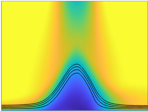
Figure 1. (a) Pressure coefficient and (b) friction coefficient in Pargal et al. (2022) (——, thick solid black), Wu et al. (2019) (– – –, red dashed line), Wu & Piomelli (2018) (- - -, light grey dotted line) and Na & Moin (1998) (- - -), compared with original data of Wu & Piomelli (2018) and Na & Moin (1998) ($\circ$). (c) Contours of mean streamwise velocity normalized by $U_{e}$ (at the reference location) in the Wu & Piomelli (2018) case, with streamlines shown at streamfunction values of $\psi _o=0.5$, 1, 1.5 and 2.

Figure 1 shows the variation of the mean wall-pressure coefficient, $C_p=(\,\bar {p}|_{y=0}-p_{e,o})/(0.5\rho U_e^2)$, and skin friction coefficient, $C_f=(u_\tau /U_e)^2/2$, where $p_{e,o}$ is the edge static pressure at the location of $x=0$, which corresponds to the reference (ZPG) location defined in each of the studies. In figure 1(b), the value of $C_f$ is normalized by its value at the reference location to better compare all cases. Only simulated cases are presented as the boundary-layer parameters for a continuous range of $x$ are available. Figure 1(a) shows that the variations of $C_p$ in the flat-plate (Pargal et al. 2022) and aerofoil (Wu et al. 2019) cases are very similar. In figure 1(b), the variations of $C_f$ are shown to match overall for these two cases, with some differences due to the convex wall curvature and trailing-edge effects (Messiter 1970). These comparisons are discussed in Pargal et al. (2022), showing that the convex curvature on the pressure side of the aerofoil does not lead to significant changes in $C_p$ and $C_f$. In the cases of Na & Moin (1998) and Wu & Piomelli (2018), where the flows undergo free-stream suction and blowing, the $C_p$ variation indicates three phases of a separated boundary-layer flow (marked in figure 1b): 1. attached APG flow, 2. separated region and 3. reattached flow under FPG. This is also reflected in $C_f$ variations: $C_f$ first decreases toward zero in the APG region, reaching negative values in the separated-flow region, and increases near the flow reattachment in the FPG region. The fact that $C_f$ reaches zero in separated flows suggests that the use of $\tau _w$ to non-dimensionalize the pressure in some existing WPS models is problematic in these flows. The contour of mean streamwise velocity of the case of Wu & Piomelli (2018) in figure 1(c) confirms these flow stages. The coefficients are compared between the results of the present rerun simulations and those of the original studies (Na & Moin 1998; Wu & Piomelli 2018); good match is obtained in both cases. The difference in $C_p$ values near $x/\theta _o\approx 200$ in the Wu & Piomelli (2018) data in figure 1(a) is due to the different definitions of the boundary-layer edge employed in the present study and that in the original study.

In figure 2, the variations of boundary-layer thickness ($\delta$), momentum thickness ($\theta$) and displacement thickness ($\delta ^*$) along the streamwise direction are shown. These thicknesses are used as inputs in several existing wall-pressure spectral models. As expected with an increase in APG, the boundary layer becomes thicker. For the cases with suction and blowing, the thicknesses reach their maxima near the end of the APG zone and then decrease with FPG. The development of the shape factor, $H$, in figure 2(d) shows a similar response, which reflects that the displacement thickness is more sensitive to the pressure gradients compared with the momentum thickness. Reynolds numbers based on different velocity scales that have been used in some wall-pressure spectral models are also compared. The one based on the inner velocity, $Re_{\tau }=u_\tau \delta /\nu$ (where $\nu$ is the kinematic viscosity) shows a similar trend as that of $C_f$ (figure 2e), while the one based on edge velocity, $Re_{\theta }=U_e \theta /\nu$, shows a variation similar to that of $\theta$ (figure 2f). The DNS cases are conducted in low Reynolds numbers ($Re_\theta \approx 300$ to 1200), while higher values are reached for the LES case ($Re_\theta \approx 2000$ to 7000).

Figure 2. Boundary-layer parameters in Pargal et al. (2022) (——, solid black), Wu et al. (2019) (– – –, red dashed line), Wu & Piomelli (2018) (- - -, light grey dotted line) and Na & Moin (1998) (- - -).

Figure 3 shows the streamwise developments of two boundary-layer parameters that are used in most existing WPS models to sensitize the modelled spectrum to the Reynolds number and the pressure gradient: $R_t\equiv Re_\tau (u_\tau /U_e)$ (figure 3a) and $\beta$ (figure 3b), respectively. As the separation point is approached, $R_t$ tends to 0 and $\beta$ to infinity. This indicates issues in many existing WPS models when used for strong-APG flows near incipient separation (Caiazzo et al. 2023), which are examined in detail in § 5.1.

Figure 3. Development of $R_t$ and $\beta$ in Pargal et al. (2022) (——, solid line), Wu et al. (2019) (– – –, red dashed line), Wu & Piomelli (2018) (- - -, light grey dotted line) and Na & Moin (1998) (- - -). For the Wu & Piomelli (2018) and Na & Moin (1998) cases, only the attached-flow region upstream of the separation point is shown; - - - (vertical): location of separation point.

For most of the experimental datasets, streamwise variations of the boundary-layer parameters are available at discrete locations only. Representative values of $Re_\theta$, $H$, $C_f$ and $\beta$ are tabulated in table 2. Specifically, the datasets of the Hu (2018) experiments contain five cases: one ZPG flow, three APG flows with $\beta$ varying from 4 to 12 and one FPG flow, at $Re_\theta = 5000$ to 11 000. The data show that the boundary-layer thicknesses (as indicated here by $Re_\theta$; for other thicknesses see the original studies) and the shape factor increase with APG and decrease in FPG, whereas $C_f$ decreases with APG and increases in FPG. The cases from Fritsch et al. (2022b) are non-equilibrium APG and FPG flows but with comparatively milder APG compared with Hu (2018). As a result, the variations in boundary-layer parameters are more limited. Also included are measurements by Goody & Simpson (2000), which were carried out for ZPG flows only but reached higher Reynolds numbers.

Table 2. List of experimental datasets and values of boundary-layer parameters at measurement locations of available data. For the Hu (2018) and Fritsch et al. (2022b) datasets, the angle of attack of the aerofoil imposed to generate the mean pressure gradient is indicated.

4. Wall-pressure statistics

In this section, the development of wall-pressure statistics along $x$ is discussed using the datasets. Different normalizations are used to analyse the wall-pressure scaling. Effects of pressure gradient, boundary-layer separation and reattachment on the WPS are examined. The goal is to (i) identify the appropriate scalings to be used in the WPS model for attached and separated flows and (ii) examine the changes of WPS due to strong pressure gradients or separation, which will be shown to be well predicted by the new model in § 5.2.

The streamwise variations of the root-mean-square (r.m.s.) of wall-pressure fluctuations and the local maximum magnitude of the Reynolds shear stress profile ($|\overline {u'v'}|_{max}$) are compared in figures 4(a) and 4(b), respectively. Both quantities are normalized by their specific values at $x=0$. Only numerical data are shown as, for experimental datasets, $p_{rms}(x)$ and $|\overline {u'v'}|_{max}(x)$ are not available. Convex wall curvature and the trailing-edge effect (Messiter 1970) intensify the wall-pressure fluctuations, as shown by the comparison between the flat-plate case of Pargal et al. (2022) and the aerofoil case of Wu et al. (2019) for $x/\theta _o>200$. In the separated-flow region, a drop in wall-pressure fluctuations is seen, which was also observed by Abe (2017). The dip is attributed to the departure of turbulent eddies from the wall, with mainly large recirculating eddies interacting with the near-wall region. As the separated shear layer reattaches, the re-emergence of intense turbulent motions near the wall leads to an augmentation of wall-pressure fluctuations, shown by the $p_{rms}(x)$ maximum shortly after the reattachment point (at $x/\theta _o\approx 280$ for Wu & Piomelli (2018) and $x/\theta _o\approx 500$ for Na & Moin 1998). Interestingly, figure 4(b) shows that the $x$ variation of the local maximum magnitude of the Reynolds shear stress profile, $|\overline {u'v'}|_{max}(x)$, is very similar to that of $p_{rms}$: the decrease near the separation point and the peak near the flow reattachment occur at almost the same $x$ locations downstream from the reattachment point, as the flow recovers towards the equilibrium ZPG flow, both $p_{rms}$ and $|\overline {u'v'}|_{max}$ reduce towards the ZPG values at $x=0$.

Figure 4. (a) Wall-pressure root mean square normalized by its value at the reference location and (b) local peak magnitude of the Reynolds shear stress, normalized by its value at the reference location, in Pargal et al. (2022) (——, solid line), Wu et al. (2019) (– – –, red dashed line), Wu & Piomelli (2018) (- - -, light grey dotted line) and Na & Moin (1998) (- - -).

To identify the best pressure scale to use in a WPS model for strong-pressure-gradient flows, in figure 5 different quantities are used to normalize the wall-pressure r.m.s. as it varies along $x$, for the datasets shown in figure 4. The r.m.s. normalized by $\tau _w$ (figure 5a) increases with APG and tends towards infinity as the separating point is approached. The use of $\tau _w$ to scale $p_{rms}$ in WPS models is, therefore, inappropriate for strong-APG boundary layers. The r.m.s. normalized by $q_e=0.5\rho U_e^2$ (figure 5b) displays a significant increase in the APG zone before the flow separation. This is because wall-pressure fluctuations are augmented in the APG region, while the edge velocity decreases. In comparison, $p_{rms}/(\rho |\overline {u'v'}|_{max})$ stays almost constant as long as the boundary layer is attached, regardless of the pressure gradient (figure 5c). In the separated-flow regions, however, a dip of $p_{rms}/(\rho |\overline {u'v'}|_{max})$ is observed, caused by a faster damping of $p_{rms}$ inside the recirculation bubble than that of the Reynolds shear stress in the detached shear layer (as shown in figure 4). These observations indicate that the wall-pressure r.m.s. scales better with $\rho |\overline {u'v'}|_{max}$ than with $q_e$ or $\tau _w$, in attached flows under strong pressure gradients, suggesting that the wall pressure fluctuation magnitude is closely correlated with active turbulent motions and that $\rho |\overline {u'v'}|_{max}$ should be used as the pressure scale in a WPS model; similar observations were made by Na & Moin (1998), Abe (2017) and Caiazzo et al. (2023). However, the appropriate wall-pressure r.m.s. scaling for the separated flow region remains to be found; but this is out of the scope of the present work.

Figure 5. Wall-pressure r.m.s. normalized by (a) local wall shear stress ($\tau _w$), (b) local dynamic pressure ($q_e$) and (c) local peak magnitude of Reynolds shear stress. (a), - - - (vertical) Shows locations of separation points. In (b,c), separated-flow regions are marked. Datasets include Pargal et al. (2022) (——, solid line), Wu et al. (2019) (– – –, red dashed line), Wu & Piomelli (2018) (- - -, light grey dotted line) and Na & Moin (1998) (- - -).

The PSD of the wall-pressure fluctuations (denoted by $\phi _{pp}$) is computed for all simulated and experimental cases and compared in figure 6. Only attached-flow regions, with ZPG or non-equilibrium APG, are considered here. The $x$ location, $\beta$ value and legend for each PSD curve in figure 6 are listed in table 3. Different normalizations are compared. Both $Re_{\theta }$ ($Re_{\theta }=300$ to 23 400) and $\beta$ ($\beta =0$ to $200$) vary greatly among these data. The high $\beta$ values occur near the separation points. In the following discussion, it will be shown that a robust set of scales to be used for strong-pressure-gradient flow WPS modelling is $\rho |\overline {u'v'}|_{max}$ as the pressure scale, $\delta$ as the length scale and $U_e$ as the velocity scale.

Figure 6. (a–c) Power spectral density of wall-pressure fluctuations for attached-flow datasets with ZPG and APGs listed in table 3, under three different scalings involving $\rho |\overline {u'v'}|_{max}$ (as the pressure scale) and outer scales: (a) $\rho |\overline {u'v'}|_{max}$, $\delta$ and $U_e$, (b) $\rho |\overline {u'v'}|_{max}$, $\delta ^*$ and $U_e$ and (c) $\rho |\overline {u'v'}|_{max}$, $\theta$ and $U_e$. Other normalizations with (d) outer scales ($q_e$, $\delta$ and $U_e$), (e,f) inner scales ($\tau _w$, $\delta _{\nu }$ and $u_\tau$, with ZPG profiles shown separately in (f) demonstrating high-frequency collapse) and (g,h) mixed scales ($\tau _w$, $\delta$ and $U_e$, with ZPG profiles shown separately in (h) demonstrating low-frequency collapse). The PSD is evaluated in dB, defined as $10\log _{10}(\phi _{pp})$. Legend is listed in table 3.

Table 3. Datasets in attached-flow regions (under ZPG, APG or FPG) that are considered in analyses of the wall-pressure spectrum.

Figure 6(a) compares the results using $\rho |\overline {u'v'}|_{max}$ as the pressure scale, $\delta$ the length scale and $U_e$ the velocity scale (or equivalently $p_{rms}$, $\delta ^*$ and the Zagarola–Smits velocity, as shown by Caiazzo et al. 2023). Note that in the experimental datasets the Reynolds shear stress data were missing. For these experimental datasets, the wall shear stress ($\tau _w$) at a mild-APG ($\beta <1$) location immediately upstream of the APG region, instead of the local Reynolds shear stress, is used to form the pressure scale for the strong-APG region. This approximation for the experimental datasets is based on the observation that $|\overline {u'v'}|_{max}(x)$ does not vary significantly in the attached-flow region upstream of the separation point, as shown previously in figure 4(b). The value of $|\overline {u'v'}|_{max}(x)\approx |\overline {u'v'}|_{max}(0)$ can then be approximated as $\tau _w(0)$ due to the existence of a constant-stress layer in a boundary layer under zero or mild pressure gradients. The treatment mentioned above is employed for the experimental cases only. Under such normalization, figure 6(a) shows that approximate low-frequency collapse is obtained. There is a small spread (within 3 dB for numerical datasets and within 4 to 5 dB for experimental ones); but this is a better low-frequency collapse as compared with results using other sets of scalings, as shown in figure 6(b–e,g). The approximate collapse is expected as the low-frequency contents are the main contributor to $p_{rms}$, which in turn scales with $\rho |\overline {u'v'}|_{max}$. Swapping the length scale for $\delta ^*$ or $\theta$, however, gives more scatter in the low-frequency range (figure 6b,c), as also shown by Caiazzo et al. (2023). Even though previous works (Kamruzzaman et al. 2015; Abe 2017; Caiazzo et al. 2023) have shown $\rho |\overline {u'v'}|_{max}$ to be the best pressure scaling for wall-pressure spectra, most of them were limited-to-low-Reynolds-number cases with mild pressure gradients. The comparison here shows that the chosen set of scaling collapses low-frequency portion of the PSD for a large range of Reynolds number with strong non-equilibrium APG as well.

In addition, figure 6(a) shows that a strong APG leads to a milder overlap-range decay rate (as compared with the ZPG rate of around $-0.8$). In addition, the high-frequency $\omega ^{-5}$ relation is shown to apply under a strong APG. The datasets, however, do not reach a sufficiently low frequency range to examine the APG effect on the $\omega ^2$ relation observed in ZPG flows for $\omega \delta /U_e<0.1$ (see, for e.g. Goody 2004).

Figure 6(e) shows that normalization based on inner velocity and length scales (i.e. using $\tau _w$, $\delta _{\nu }\equiv \nu /u_\tau$ and $u_{\tau }$) gives a high-frequency collapse for the ZPG spectra (see ZPG profiles shown separately in figure 6f), but a large scatter for the APG ones. When mixed variables are used (i.e. using $\tau _w$, $\delta$ and $U_e$ as shown in figure 6g), which is commonly applied in existing WPS models, the low-frequency range collapses for the ZPG spectra only (see ZPG profiles shown separately in figure 6h), but not for cases with strong APG, as $p_{rms}$ does not scale with $\tau _w$. On the other hand, normalization based on outer variables only (i.e. using $q_e$, $\delta$ and $U_e$ as shown in figure 6d) gives a better collapse than that based purely on the inner variables; however, it still fails to collapse the low-frequency range. Based on these observations, the best $\phi _{pp}$ scaling among these options is thus $(\rho |\overline {u'v'}|_{max})^2\delta /U_e$.

The effects of Reynolds number (in combination with effects of APG) are analysed next. Figures 7(a)–7(c) categorize the wall-pressure PSDs in APG and ZPG flows into three Reynolds-number groups: low-$Re_\theta$ ($Re_\theta \approx 300$ to 1000), mid-$Re_\theta$ ($Re_\theta \approx 2000$ to 8000) and high-$Re_\theta$ ($Re_\theta \approx 8000$ to 23 400) groups. Note that in the high-$Re_\theta$ group, only ZPG or mild-APG flows are available in the present datasets. Figure 7(a) shows that all low-$Re_\theta$ spectra collapse well in the majority of the frequency range. This is because the overlap range is limited and the low-frequency range is well collapsed by using $\rho |\overline {u'v'}|_{max}$ as the pressure scaling. The CD aerofoil data (– – –, Wu et al. 2019) give high-frequency WPS levels that are slightly higher than the flat-plate data (——, Pargal et al. 2022) with matching Reynolds number and pressure gradients. The difference is attributed to the effects of surface curvature and the aerofoil trailing edge on the WPS, which are shown by figure 7(a) to be relatively weak compared with the effects of the Reynolds number and pressure gradients. At higher Reynolds numbers, the overlap range appears and grows with $Re_\theta$ (figure 7b,c). The width of the overlap range is shown to decrease with APG and the slope of this range becomes steeper with APG.

Figure 7. Wall-pressure PSDs in APG boundary layers with different Reynolds-number ranges: (a) low-$Re_\theta$ range ($Re_{\theta }=300$ to $1000$), (b) mid-$Re_\theta$ range ($Re_{\theta }=2000$ to $8000$) and (c) high-$Re_\theta$ range ($Re_{\theta }=8000$ to 23 400). (d) The PSDs in FPG flows (blue) compared with ZPG ones (grey). See table 3 for legend.

The PSDs in FPG flows are shown in figure 7(d) using the two FPG datasets (in blue) of Hu (2018) and Fritsch et al. (2022b), as compared with the corresponding ZPG spectra (in grey) from these two studies. Under $\beta \approx -0.5$, both spectra show a milder slope in the overlap range than the ZPG spectra. This is consistent with the steeper slope in APG flows discussed above. In addition, the overlap ranges are slightly widened under FPG with the low-frequency limit moving towards lower frequencies, especially for the lower-Reynolds-number case (Hu 2018, blue circles). This is associated with a weaker mean-flow wake region under FPG.

To analyse the WPS associated with separated and reattached flows, figures 8(a) and 8(b) compare the spectra extracted, respectively, from the separated-flow regions and the regions downstream of the boundary-layer reattachment in the cases of Na & Moin (1998) and Wu & Piomelli (2018). These two datasets are included as they are the only ones in the present collection that include separated flows. Figure 8(a) shows that, in the separated-flow regions, both overlap-range and high-frequency wall-pressure fluctuations are reduced compared with those in respective reference ZPG locations (dashed lines), due to the departure of intense turbulent motions from the wall following the detachment of the shear layer. The scaling does not collapse the low-frequency range as it does for attached flows. This is expected as the wall-pressure r.m.s. does not scale with $|\overline {u'v'}|_{max}$ in this region (figure 5c). However, it is interesting that the shape of the spectrum does not vary significantly in the separated-flow region: the spectra in figure 8(a) all display a narrow low-frequency peak with greatly reduced high-frequency contribution. This observation provides insight into WPS modelling in separated flows, to be used in § 5.2.

Figure 8. (a) Wall-pressure PSDs in separated-flow regions (——, thick solid line) compared with those at respective reference ZPG locations (– – –); grey lines show Wu & Piomelli (2018) data at $x/\theta _o = 150$, 175, 200, 220 and 240; black lines show Na & Moin (1998) data at $x/\theta _o=270$, 300 and 400. (b) Wall-pressure PSDs in reattached-flow region of Wu & Piomelli (2018) at $x/\theta _o = 275$, 300, 350 and 450. In both (a,b), increase in line thickness indicates downstream direction.

Downstream of the reattachment point, figure 8(b) shows that the spectrum recovers gradually from the low-frequency-dominant state inside the separated-flow region towards the equilibrium state, with augmented mid- to high-frequency contents.

5. Wall-pressure spectra modelling

5.1. Performance of existing wall-pressure spectral models

Most existing wall-pressure spectral models are developed for regions with zero and adverse pressure gradients. Figure 9 compares a number of existing WPS models introduced in § 1 against the present datasets of ZPG and APG (attached regions only) flows (marked by blue solid lines) for six different $Re_\theta$-$\beta$ combinations. Among them, figures 9(e) and 9(f) show two examples near boundary-layer separation. The models and their legend are listed in table 4, including a proposed model (shown by red solid lines) to be formulated in § 5.2 to address the issues of the existing models observed in this section. All model predictions are re-normalized with the optimal $\phi _{pp}$ normalization ($\rho |\overline {u'v'}|_{max}$, $U_e$ and $\delta$) identified in § 4. The comparison of the measurement results among these six flows demonstrates dependencies of the WPS on the APG and the Reynolds number, as discussed in § 4. Under the present normalization, the main variations are in the width and slope of the overlap range.

Figure 9. Comparison between predictions of WPS models and numerical or experimental measurements (——, blue solid line), for different types of flow: (a) ZPG, high-$Re_\theta$ flow (Fritsch et al. 2022b, $2^\circ$), (b) weak-APG, high-$Re_\theta$ flow (Fritsch et al. 2022b, $12^\circ$), (c) strong-APG, low-$Re_\theta$ flow (Wu et al. 2019), (d) very-strong-APG flow at intermediate $Re_\theta$ (Wu & Piomelli 2018), (e) flow near separation point at a low $Re_\theta$ (Na & Moin 1998) and (f) flow near separation point at an intermediate $Re_\theta$ (Wu & Piomelli 2018). Predictions of all models are re-normalized by $\rho |\overline {u'v'}|_{max}$, $U_e$ and $\delta$ for comparison purposes. Legend of model results is given in table 4. The proposed model (——, red solid line) will be introduced in § 5.2.

Table 4. List of WPS models examined with the present datasets.

First, the overall performance of the WPS models in predicting the wall-pressure fluctuation intensity is analysed based on the predicted $p_{rms}$ value. Table 5 lists the prediction error of each of the tested model in the six flows examined in figure 9. Good $p_{rms}$ predictions (with errors up to 26 %) were made by all models in the ZPG flow (row a). Under stronger APG (with $\beta$ up to 23, rows b,c), over- or under-prediction by a large fraction (40 % to 60 %) is seen in four out of the five existing models. However, in flows with very strong APG, including the region near the separation point (rows d–f), very large errors are seen in all five existing models, as they were not formulated or calibrated for non-equilibrium strong-APG flows. The proposed model calibrated from some of these flows, on the other hand, is shown to reproduce very well the $p_{rms}$ values (with up to 8 % error) in all six flows. A good prediction of wall-pressure fluctuation intensity does not necessarily mean equally good prediction in the WPS shape, which is analysed next. The large model errors in rows (d) to (f) are also explained below.

Table 5. Wall-pressure r.m.s. prediction errors from the existing models tested and the proposed models, examined for the six flows in figure 9. The error is calculated as $(\,p_{rms}-p_{rms,a})/p_{rms,a}$, where $p_{rms,a}$ is the actual value from measurement. Rows (a)–(f) correspond to the flows in figure 9(a–f), respectively. In (e,f), the Lee (2018) and Rozenberg et al. (2012) models yield undefined values from double-precision floating-point number operations.

In a ZPG flow (figure 9a), almost all existing models (except the Kamruzzaman et al. (2015) model) give overall good predictions in the spectrum. For the weak-APG flow (figure 9b), the tested models are shown to give reasonably good predictions overall. Goody's model over-predicts mid-to-high-frequency WPS content due to lack of sensitivities of the overlap-range width and slope to the pressure gradient. Kamruzzaman et al. (2015) model does not produce an overlap range and, as a result, yields significantly under-predicted high-frequency contents. Moreover, except for the Hu (2018) model, all existing models give noticeable differences in the overlap-range slope from the experimental measurement.

For the flow under relatively weak APG ($\beta \approx 8$), figure 9(c) shows that the Rozenberg et al. (2012) and Lee (2018) models give very good overall predictions of the spectrum, whereas the Hu (2018) and Kamruzzaman et al. (2015) models under-predict the WPS at low frequencies. The Goody (2004) model under-predicts the WPS in the whole frequency range, which is expected, as this model was developed and calibrated for ZPG flows only.

In strong-APG flows (figure 9d–f), especially near the boundary-layer separation point, the existing models give large errors. This is because of the model parameters used in these models: $R_t$ and $\beta$ tend towards zero and infinity, respectively. Another source of error is the inappropriate pressure scaling (i.e. $\tau _w$) used in the models. For instance, Rozenberg et al. (2012) model

(5.1)\begin{equation} \frac{\phi_{pp} (\omega) U_e}{\tau_w^2 \delta^*}=\frac{0.78(1.8\varPi \beta+6)(\omega \delta^*/U_e)^2}{[(\omega \delta^*/U_e)^{0.75}+C_1']^{3.7}+[C_3'(\omega \delta^*/U_e)]^7}, \end{equation}

where $C_3'=3.76R_T^{-0.57}$, reaches a singularity as $\tau _w$ and $R_t$ become zeros and $\beta$ becomes infinity. Employing $\tau _w$ as the pressure scale for $\phi _{pp}$ also renders the dimensionless spectrum excessively sensitive to strong APGs, even if the flow stays attached. This issue is common in existing models. In addition, most of these models were fitted to limited types of flows, such as low-Reynolds-number aerofoil boundary layers in Kamruzzaman et al. (2015), flat-plate boundary layers in Hu (2018) and ZPG flows in Goody (2004). Moreover, sometimes the boundary-layer flow properties used for model calibration were estimated from lower-fidelity methods such as XFOIL or RANS calculations, as opposed to DNS/LES or experimental measurements. In § 5.2, these limitations are addressed to develop a well-behaved WPS model for both ZPG and APG flows, which can be attached or separated.

5.2. A new generalized WPS model for non-equilibrium boundary layers

In this section, a new wall-pressure spectral model is developed, with the Goody (2004) model as a base. First, various components of the modification are introduced and justified. Then, prediction of the new model is compared with the datasets, first for attached APG flows and next for separated flows, reattached flows and FPG flows. Finally, a sensitivity analysis of the new model prediction to the model parameters is carried out, to verify that the intended dependencies are indeed captured.

The Goody (2004) model is a good starting point as it has been shown to be successful in WPS prediction for ZPG boundary layers; it is also relatively simple compared with some other existing models. In summary, the Goody (2004) model is modified by removing the Reynolds-number parameter ($R_t$) and using model inputs that derive directly from the local mean velocity distribution, $U^+(x,y)$. Only inputs that are quantifiable from engineering predictive approaches (such as RANS models) are considered, so the model is of practical use in engineering applications. The dependence of these inputs on the $U(y)$ distribution at a given $x$ location allows the model to sense the local state of the turbulent boundary layer.

The Goody (2004) model reads

(5.2)\begin{equation} \tilde{\phi}_{pp}\left(\tilde{\omega}\right) =\frac{a\tilde{\omega}^b}{(h\,\tilde{\omega}^c+d)^{e}+(\,f \mathcal{F}\,\tilde{\omega})^g}, \end{equation}

where $\tilde {\phi }_{pp}=\phi _{pp}/\phi _{pp}^*$ and $\tilde {\omega }=\omega /\omega ^*$ are dimensionless WPS and frequency, respectively, based on a spectrum scale of $\phi ^*_{pp}$ and a frequency scale of $\omega ^*$, as listed in table 6. The coefficients $a$ to $h$ and the function $\mathcal {F}$ are defined in table 6. The model was developed based on the observed dependencies of the low-frequency spectrum on the outer scales, as well as that of the high-frequency spectrum on the inner scales, in a ZPG or weak-pressure-gradient flow. The model was known to predict well the overlap range of the spectrum for ZPG boundary layers (as also shown in figure 9a), which depends on the Reynolds number only. The dependence is captured by including $R_t$ in the model. However, the overlap-range spectrum also depends on the pressure gradient in strong-pressure-gradient boundary layers. In figure 10(a), the prediction of the original Goody's model is examined at several $x$ locations of the Wu & Piomelli (2018) case in the attached-flow region with weak to strong APGs. In this region, $\beta$ ranges from 0 to 200 and $Re_{\theta }$ is from 2000 to 6000. With the increase in APG, Goody's model shows increasing under-prediction in the whole frequency range.

Table 6. Comparison between Goody (2004) model and the proposed model. The parameters $\phi _{pp}^*$ and $\omega ^*$ are the chosen scalings for WPS and frequency, respectively. Special treatments for a flow region characterized by a separated boundary layer or a limited logarithmic layer are listed.

Figure 10. Comparison between model predictions of (5.2) with progressive changes described in text (——, red solid line) and Wu & Piomelli (2018) (——, thick solid line) data in attached flows with weak to strong APGs, to show improvement brought by each model change. (a) The Goody (2004) model (predictions are plotted using the optimal normalizations), (b) pressure scale changed from $\tau _w$ to $\rho |\overline {u'v'}|_{max}$, (c) additionally replacing dependency on $R_t$ with that on $y_w^+$, (d) further addition of Coles’ parameter. Thicker lines indicate increase in $x$ (corresponding to increasing $\beta$).

Table 6 lists the changes from the original Goody (2004) model to the proposed model. The modified expressions of the model parameters were obtained by fitting a subset of the datasets: the APG and ZPG data of Pargal et al. (2022), Wu & Piomelli (2018), Hu et al. (2013), Fritsch et al. (2022b) and Goody (2004), as well as separated-flow data of Na & Moin (1998) and Wu & Piomelli (2018). Datasets that were not used for model development were used in testing the model in figure 9(c,e,f) for attached APG flows, figure 13(b) for a reattached flow and figure 14(b) for a FPG flow.

In the following, the main changes are introduced and progressively applied to demonstrate the improvement of each of them. First, the pressure scale (i.e. $\tau _w$) on the left-hand side of (5.2) is replaced with $\rho |\overline {u'v'}|_{max}$, with the additional change of replacing the constant $d=0.5$ with 0.7 for a better low-frequency collapse with the current data. The effect of these modifications is shown in figure 10(b), where the low-frequency range is shown accurately predicted for all $x$ locations. The use of $\rho |\overline {u'v'}|_{max}$ ensures that the spectral values are finite near the separation point.

Next, to capture the variation of overlap and high-frequency range in APG flows, a new parameter is needed to replace $R_t$ to model the width change of the overlap range. Past studies showed that turbulent fluctuations in the logarithmic layer form the main contributor to the overlap range of the WPS. For example, Farabee & Casarella (1991) showed that, for ZPG boundary layers, with an increase in Reynolds number accompanied by a thickening of the logarithmic layer, the WPS overlap range becomes wider and its integral contribution to $p_{rms}^2/\tau _w^2$ varies as $6.5+1.85\ln (Re_{\tau }/333)$ at sufficiently high Reynolds numbers. Additional evidence in APG flows is provided by Jaiswal et al. (2020), who showed that the logarithmic layer yields the highest contribution to the overlap range of $\phi _{pp}$ based on analyses of the velocity sources of the wall-pressure Poisson equation. Here, a new model input is introduced: $y_w^+(x)$, defined as the local elevation of the upper edge of the logarithmic layer, to sensitize the model spectrum to the change in logarithmic-layer thickness due to Reynolds number and/or pressure gradients. The subscript $w$ in $y_w$ represents the width of the logarithmic layer. Specifically, the term $1.1R_t^{-0.57}$ is replaced with $(y_w^+)^{-0.37}$. The new expression is obtained by assuming a power function of $y_w^+$ and performing a nonlinear least square fit (using both ZPG and APG datasets) to calculate the exponent.

The parameter $y_w^+(x)$ is dynamically determined based on the boundary-layer mean velocity, $U(x,y)=\bar {u}$, as the $y^+$ location where $U^+(x,y) -[\kappa (x)^{-1} \log y^+ + B(x)]$ departs from $0$ at the upper limit of the logarithmic layer (as shown in figure 11c). Here, $\kappa$ is the von Kármán constant and $B$ is the log-law intercept, both of which are allowed to vary along $x$ in a non-equilibrium boundary layer. Note that, due to the use of local viscous scaled units in $y_w^+$ and $U^+$ etc., the present modification needs special treatment at the separation point and inside the separated-flow region, which will be discussed later. To determine $\kappa (x)$, the diagnostic function $I(x,y)=y^+ \partial U^+/\partial y^+$ (figure 11b) is calculated from the mean velocity profile (figure 11a) for data of Wu et al. (2019). The local minima of $I(x,y)$ at a given $x$ is taken as $1/\kappa (x)$. Following the determination of $\kappa (x)$, $B(x)$ is calculated using $U^+(x,y) -[\kappa (x)^{-1} \log y^+ + B(x)]=0$. Figure 11(d) shows that the correlation between $\kappa (x)$ and $B(x)$ obtained for all cases in the present attached-flow datasets is consistent with that observed by Nagib & Chauhan (2008) from a large collection of flows with or without pressure gradients. As shown in figure 10(c) compared with figure 10(b), the modelling of overlap-range width based on $y_w^+$ is successful for the present APG datasets: the high-frequency range is now better predicted with the corrected width. As the APG becomes stronger, $y_w^+$ decreases as shown in figure 11(c), reducing the overlap-range width as shown in figure 10(c). The main WPS prediction error is now predominantly an inaccurate slope of the overlap range, as shown in figure 10(c).

Figure 11. (a–c) Calculation of $\kappa (x)$, $B(x)$ and model parameters shown using Wu et al. (2019) data at locations $x/\theta _o=50$, 105, 120 and 130. Increasing line thickness indicates increase in $x$. (a) Mean velocity profiles in inner units. (b) Diagnostic function, $I=y^+\partial U^+/\partial y^+$. (c) Velocity profiles with logarithmic relation subtracted. Calculations of $\kappa$, $\varPi$ and $y_w^+$ are indicated for $x/\theta _o=105$ in (b,c). (d) Correlation between calculated $\kappa B$ and $B$, compared with the fitted relation from Nagib & Chauhan (2008) (– – –, dashed line): $\circ$ (red) Wu & Piomelli (2018) (attached flow before separation), $\circ$ Wu & Piomelli (2018) (attached flow downstream of reattachment), $\Diamond$ (red) Hu (2018), $\times$ (red) Fritsch et al. (2022a), $+$ (red) Goody (2004), $\square$ (red) Pargal et al. (2022), $\triangleright$ (red) Wu et al. (2019) and $\Delta$ (red) Na & Moin (1998).

The change in WPS overlap-range slope (in addition to the change of the width of this range as is characterized by $y_w^+$) is assumed to be caused by the variation in the strength of the outer-layer turbulent motions. This assumption arises from the understanding that an APG leads to more energized large turbulence motions in the outer layer and a thinner logarithmic layer. In addition, an APG is known to cause an increase in low-frequency WPS contents and a decrease in mid-to-high-frequency ones (e.g. Rozenberg et al. 2012; Catlett et al. 2016; Lee 2018), which is reflected in a steeper overlap-range slope. To account for the variation in the strength of the wake region, an additional model input is used: Coles’ parameter, $\varPi (x)$. An augmentation of $\varPi$ signals stronger turbulent intensity and mixing in the outer layer. Here, $\varPi (x)$ is evaluated based on $U^+(x,y)$, by measuring the peak value of $U^+ -[\kappa ^{-1} (\log (y^+) + B)]$ (as shown in figure 11c) and dividing it by $2/\kappa (x)$. In the generic model form in (5.2), the coefficient $c$ is known to impose the slope of the overlap range of $\phi _{pp}$ (Rozenberg et al. 2012; Lee 2018; Thomson & Rocha 2022). The present datasets suggest that $c$ is a function of both $y_w^+$ and $\varPi$: for flows with larger $y_w^+$ values, the same pressure gradient difference leads to a larger slope variation compared with cases with smaller $y_w^+$ values. Therefore, the constant $c$ is replaced by a function of both $\varPi$ and $y_w^+$. A posynomial functional form is assumed; the constant coefficients and exponents are fitted based on the present datasets. Additionally, for boundary layers with very strong APG or near the separation point, the logarithmic layer diminishes and the WPS overlap range is very narrow or absent. At these flow locations the modelled WPS is weakly sensitive to the $c$ value. The present datasets yield a maximum value of $c\approx 0.98$ in strong-APG flows. For simplicity, $c$ is capped at 1.0. This treatment, however, may be improved in the future when more high-Reynolds-number strong-APG data become available. The final form of the generalized WPS model is

(5.3)$$\begin{gather} \frac{\phi_{pp} (\omega) U_e}{(\rho |\overline{u'v'}|_{\max})^2 \delta} =\frac{3(\omega \delta/U_e)^2}{[(\omega \delta/U_e)^c+0.7]^{3.7}+[(y_w^+)^{-0.37}(\omega \delta/U_e)]^7}, \quad \text{where} \end{gather}$$

(5.4)$$\begin{gather}c = \min\left[1.0,0.8+3.34\times 10^{-4} \varPi^{1.86} (y_w^+)^{0.76}\right]. \end{gather}$$

For the ZPG flow shown in figure 9(a), the Goody (2004) model and the proposed model give similar predictions and both compare well with the experimental measurements. The small difference between the predictions of the two models is because of the use of different model parameters and that the fitting of the proposed model is conducted for both ZPG and APG flows. For the strong-APG flows in the present datasets, figure 10(d) and figure 9 show that the generalized model predicts the WPS very well. Note, however, that the present strong-APG data used to calibrate this model are from limited-Reynolds-number flows with a rather narrow WPS overlap range. Additional data from high-Reynolds-number strong-APG flows are not available, but are needed to validate the use of the model of its present form in flows with higher Reynolds numbers.

A few scenarios require special treatments, as listed in table 6. For cases with very low Reynolds numbers and extreme APGs, which practically remove the logarithmic region from the boundary layer (i.e. if $y_w^+<15$), $y_w^+$ and $c$ are set to constant values: $y_w^+=15$ and $c=0.85$ as calibrated from the present datasets, to reflect the insensitivity of $\phi _{pp}$ to either Reynolds number or pressure gradient, as shown in figure 7(a). Moreover, in case of boundary-layer separation, modification of the model is needed for $x$ locations at the separation point and inside the separation bubble. Inspired by the similar WPS profiles across the normalized frequency range in the separated region as shown in figure 8(b), $y_w^+$ and $c$ are set to constants: $y_w^+=2$, $c=0.75$, and $d$ is set to 0.5 (table 6), calibrated based on the data of Na & Moin (1998) and Wu & Piomelli (2018). The separation modification is activated for $x$ regions where $C_f(x)$ is calculated as zero or negative, corresponding to the region of mean-flow separation. With the aforementioned separated-flow treatment, the proposed model is evaluated at a number of streamwise locations inside the separation regions of the flows of Na & Moin (1998) and Wu & Piomelli (2018) in figure 12. The WPS prediction does not vary with $x$ in this region, since the model parameters are set to constants. Overall good comparison with the simulation data is achieved. Although the separation treatment introduces a discontinuity in $c$ value at the separation point (as $c$ approaches 1 towards the point while $c=0.75$ at that point), it is shown not to affect the prediction significantly, as the overlap range is short in the strong-APG region in the vicinity of the detachment.

Figure 12. Comparison between model prediction (——, red solid line) and simulation data (—— Na & Moin (1998) and —— (light grey solid line) Wu & Piomelli 2018) in the separated-flow regions. Increasing line thickness indicates an increase in $x$ values as used in figure 8(a).

Although the model is primarily developed for attached or separated APG flows, it is examined in other regions of a non-equilibrium boundary layer to explore its extendibility to more universal applications. First, the model is evaluated in the region downstream from the flow reattachment point until a near-equilibrium ZPG state in figure 13 against Wu & Piomelli (2018) data, at four $x$ locations between $x/\theta _o=250$ and $x/\theta _o=350$. Figure 13(a) shows that, near the reattachment point (shown by the thinnest lines), the local mean velocity departs significantly from a canonical boundary-layer profile, without a clear logarithmic layer. With increasing $x$, the logarithmic layer gradually recovers towards the equilibrium ZPG state and the overlap range of the WPS thickens gradually (figure 13b). The model is shown to capture such a trend of WPS variation. The overall spectral levels are well predicted due to the approximate scaling of $p_{rms}$ on $\rho |\overline {u'v'}|_{max}$, while the spectral shape is captured by $y_w^+(x)$ and $\varPi (x)$ representing the local thickening of the logarithmic layer and the weakening of wake, respectively, during recovery.

Figure 13. Comparison between model prediction (——, red) and Wu & Piomelli (2018) data (——) in the attached-flow region downstream of reattachment point (at $x/\theta _o$ from 250 to 350, the most downstream location corresponding to near-equilibrium flow). (a) Mean velocity profiles with the logarithmic relation subtracted; – – – (blue dashed line) value corresponding to logarithmic layer. (b) Wall-pressure PSD comparison. Increasing line thickness indicates an increase in $x$.

In addition, the model is tested in FPG flows, as shown in figure 14, against the experimental data of Hu (2018) and Fritsch et al. (2022b). Figure 14(a) shows that, under FPGs (shown in blue) as compared with the ZPG profiles (shown in grey), the main change is a reduction of $\varPi$, which leads to a milder slope of the WPS overlap range. Figure 14(b) shows that this change in WPS is globally captured well by the proposed model.

Figure 14. Comparison between model prediction (——, red solid line) and experimental data in FPG flows: $\circ$ (cyan) Hu (2018, $\beta =-0.5$) and - - - (cyan dotted line) Fritsch et al. (2022b, $\beta =-0.5$). (a) Mean velocity profile with the logarithmic relation subtracted; the ZPG profile in each of the two studies (shown in grey) is compared. – – – Value corresponding to logarithmic layer. (b) Wall-pressure PSD comparison.

Figure 15 shows results of sensitivity analyses carried out for the parameters $y_w^+$ and $\varPi$ of the proposed model. The WPS predictions obtained with $\pm 30$ % change of each of the two parameters (marked by the highlighted region) are compared with the datasets, for three types of flows with different ranges of Reynolds number and $\beta$. Figure 15(a,c,e) shows that the variation of $y_w^+$ has an effect on the overlap-range and high-frequency contents, by controlling the width of the overlap range. The effect appears to be particularly strong in a weak-APG flow. Figure 15(b,d,f) shows that $\varPi (x)$ modifies the slope of the overlap range, with the model particularly sensitive to its value in high-Reynolds-number flows where the overlap range is pronounced. These results show that the introduced parameters affect the WPS prediction in their intended ways. Furthermore, slight variations in quantifying $y_w^+$ and $\varPi$ do not significantly worsen WPS prediction.

Figure 15. The WPS prediction of the proposed model (——, red solid line) compared with measurements (——, blue solid line) in the following cases: (a,b) high-Reynolds-number and weak-APG flow (Fritsch et al. 2022b, $\beta =0.58$), (c,d) low-Reynolds-number and strong-APG flow (Wu et al. 2019, $\beta =8.3$) and (e,f) high-Reynolds-number and strong-APG flow (Hu 2018, $\beta =6$). Yellow regions mark prediction variations with $\pm 30$ % change in input parameters $y_w^+$ (a,c,e) or $\varPi$ (b,d,f). In (d), variation of $\varPi$ does not change WPS prediction as $c$ is set to a constant at this location due to $y_w^+<15$ (see table 6).

6. Conclusions and discussion

In this study, datasets collected from numerical (DNS and LES) and experimental studies are used to characterize the variation of wall-pressure statistics in various types of boundary-layer flows, attached or separated and then reattached, with zero, adverse or favourable pressure gradients at different ranges of Reynolds number. These data were used to gain insight for developing a new WPS model and to test it. Only existing datasets that contain both WPS data and wall-normal profiles of the mean velocity measured at the same streamwise locations as the WPS are considered, as these quantities are required in testing the new model. For non-zero pressure-gradient flow data, the present focus is on non-equilibrium ones. The numerical data in the datasets were validated in various flow quantities. They are not prone to errors originating from installation effects, as in many experimental studies, and are free from modelling errors, as in RANS or boundary-layer closures used in the development of some existing WPS models. Strongly non-equilibrium streamwise pressure-gradient variations are included in the datasets. By comparing different sets of variables used to normalize the WPS ($\phi _{pp}$), an optimal set of scales is identified: $U_e$, $\delta$ and $\rho |\overline {u'v'}|_{max}$, and is used for WPS model development.

The performances of various existing wall-pressure spectral models are evaluated in the flows contained in the datasets. These models are shown to fail to predict the wall-pressure spectra in non-equilibrium strong-APG flows. The failures are caused by the use of inappropriate pressure scaling ($\tau _w$), being fitted to limited types of flows and the dependencies on $u_\tau$-based model parameters, as $u_\tau$ reduces to zero at the detachment point.

Next, more robust model parameters are proposed and used to modify Goody's model. These parameters are (i) the logarithmic-layer extent, $y_w^+$, and (ii) Coles’ parameter, $\varPi$. These parameters carry information on the local state of the boundary-layer flow as found in the mean velocity profile. The parameters, together with the scaling variable $\rho |\overline {u'v'}|_{max}$, are quantifiable or inferable from turbulence models (e.g. RANS models) or experimental measurements of the mean velocity and wall friction. For APG flow experiments where the Reynolds shear stress is not directly measured, the present datasets suggest that $\rho |\overline {u'v'}|_{max}(x)$ may be approximated based on the wall shear stress at an upstream ZPG location. Using $y_w^+$ and $\varPi$ is a more direct approach to model the change in contributions from wall-layer and outer-layer turbulent flows to the WPS, compared with existing approaches based on the local pressure gradient (e.g. Clauser's parameter, $\beta$) and/or the local Reynolds number (e.g. $R_t$). As the streamwise development of the mean velocity contains the history effect of non-equilibrium pressure gradients, $y_w^+$ and $\varPi$ are measures of this history effect. In contrast, the history effect of pressure gradient is not directly represented by a local pressure-gradient parameter, such as $\beta$ which is used in some existing WPS models.

Comparison with available numerical and experimental measurements shows that the proposed model gives good predictions for ZPG, APG (attached-flow region) and FPG flows. For the two datasets with strong APGs and boundary-layer separation considered herein, the wall-pressure spectra are shown to display similar shapes and magnitudes across the separation bubble. There, the model is shown to give overall good predictions, if the overlap-range width and slope are set to constants fitted based on present data. More separated-flow data are needed to test this model, for example, in flows with various separation-bubble sizes and dynamics.

A qualitatively good prediction is also obtained downstream of flow reattachment where the boundary layer departs significantly from its equilibrium state. Hence, the new model is considered as a generalized wall-pressure spectral model for a wide range of ZPG/weak-pressure-gradient and non-equilibrium, strong-pressure-gradient boundary layers, as opposed to existing models designed for limited types of flows.

In practice, the accuracy of the proposed model used with measured inputs (e.g. from experiments or RANS simulations) depends on the accuracy of the measured quantities, including mean velocity, wall friction and (modelled or inferred) Reynolds shear stress. For example, RANS simulations may not be accurate in predicting the wall shear stress, separation point or the separation-bubble extent in an APG flow. However, this is a limitation for WPS models in general; improving turbulence closures or experimental measurements in non-equilibrium boundary layers is an important, but separate, topic. The main contributions of this work are (i) to ensure WPS model boundedness in non-equilibrium APG flows and (ii) to include local velocity-based variables to better model the history effect of pressure gradients on the WPS.