Fundamental time scales of bubble fragmentation in homogeneous isotropic turbulence

Abstract

We investigate the fundamental time scales that characterise the statistics of fragmentation under homogeneous isotropic turbulence for air–water bubbly flows at moderate to large bubble Weber numbers, $We$. We elucidate three time scales: $\tau _r$, the characteristic age of bubbles when their subsequent statistics become stationary; $\tau _\ell$, the expected lifetime of a bubble before further fragmentation; and $\tau _c$, the expected time for the air within a bubble to reach the Hinze scale, radius $a_H$, through the fragmentation cascade. The time scale $\tau _\ell$ is important to the population balance equation (PBE), $\tau _r$ is critical to evaluating the applicability of the PBE no-hysteresis assumption, and $\tau _c$ provides the characteristic time for fragmentation cascades to equilibrate. By identifying a non-dimensionalised average speed $\bar {s}$ at which air moves through the cascade, we derive $\tau _c=C_\tau \varepsilon ^{-1/3} a^{2/3} (1-(a_{max}/a_H)^{-2/3})$, where $C_\tau =1/\bar {s}$ and $a_{max}$ is the largest bubble radius in the cascade. While $\bar {s}$ is a function of PBE fragmentation statistics, which depend on the measurement interval $T$, $\bar {s}$ itself is independent of $T$ for $\tau _r \ll T \ll \tau _c$. We verify the $T$-independence of $\bar {s}$ and its direct relationship to $\tau _c$ using Monte Carlo simulations. We perform direct numerical simulations (DNS) at moderate to large bubble Weber numbers, $We$, to measure fragmentation statistics over a range of $T$. We establish that non-stationary effects decay exponentially with $T$, independent of $We$, and provide $\tau _r=C_{r} \varepsilon ^{-1/3} a^{2/3}$ with $C_{r}\approx 0.11$. This gives $\tau _r\ll \tau _\ell$, validating the PBE no-hysteresis assumption. From DNS, we measure $\bar {s}$ and find that for large Weber numbers ($We>30$), $C_{\tau }\approx 9$. In addition to providing $\tau _c$, this obtains a new constraint on fragmentation models for PBE.

1. Introduction

Fragmentation of bubbles by turbulence resulting in transfer of volume from large to small scales through a fragmentation cascade is relevant to a variety of natural and engineering applications. We consider air–water turbulent bubbly flows where the density ratio between that of the bubble ($\rho _a$) and the surrounding fluid ($\rho _w$) is $\rho _w/\rho _a\sim 1000$. While these flows often exhibit multiple physical processes that affect the number of bubbles of a given size (e.g. entrainment, degassing, dissolution, coalescence), fragmentation is critical to understanding the size-distribution of bubbles. For typical bubbly flows with macroscopic time scales large compared with those of the underlying turbulence, the distribution of large bubbles often matches an equilibrium fragmentation cascade (Garrett, Li & Farmer 2000; Deane & Stokes 2002; Deike 2022), suggesting that fragmentation dominates and rapidly reaches equilibrium. Applicable to flows with large Reynolds numbers where the length scale of the bubbles is much larger than the Kolmogorov scale but much smaller than the geometric length scales of the flow, fragmentation of bubbles within the Kolmogorov inertial subrange of homogeneous isotropic turbulence (HIT) is often studied. Recent work has shown that HIT is observed at the bubble scale even in close proximity to a free surface (Yu et al. 2019).

In HIT, fragmentation is primarily governed by the disturbing effect of turbulent fluctuations and the restoring effect of surface tension. The ratio between the two is given by the bubble Weber number

(1.1)\begin{equation} We = \frac{ 2 \varepsilon^{2/3} (2 a)^{5/3}}{\left(\sigma/\rho_w\right)} {,} \end{equation}

where $\varepsilon$ is the turbulent dissipation rate, $a$ is the parent-bubble radius and $\sigma$ is the surface-tension coefficient. As bubbles are not generally spherical, radius, $a$, of a bubble here is defined in terms of the volume, $v$, of the bubble by $a=(3v/4{\rm \pi} )^{1/3}$. The Hinze scale is defined as the Weber number $We_H$ (and corresponding radius $a_H$) below which surface tension largely prevents fragmentation (Hinze 1955). Thus, our focus is moderate ($We \gtrsim We_H$) to large ($We\gg We_H$) Weber numbers where fragmentation is present.

For $We\sim \infty$, the daughter bubbles of a previous fragmentation will themselves fragment, leading to an equilibrium fragmentation cascade with bubble-size distribution $N(a)\propto a^{-10/3}$ (Garrett et al. 2000). Here, $N(a)\delta a$ is defined to be the number of bubbles of radius $a\le a'< a+\delta a$. Using location as an analogy for bubble size, for finite $We$ the flux of air due to fragmentation can be either local, corresponding to daughter bubbles of similar size as the parent bubble and likely to further fragment, or non-local, corresponding to daughters much smaller than the parent and likely smaller than $a_H$ (Chan, Johnson & Moin 2021b). Chan et al. (2021c) measure bubbles $We\sim 20$ and demonstrate the locality of the majority of the flux, confirming the applicability of the fragmentation cascade and associated $-10/3$ power law for moderate and large $We$, where surface tension is present but does not prevent fragmentation. This $-10/3$ power law is observed in a variety of flows including emulsions (Skartlien, Sollum & Schumann 2013), breaking waves (Deane & Stokes 2002) and turbulent free-surface entrainment (Yu, Hendrickson & Yue 2020). This prevalence illustrates that fragmentation cascades are ubiquitous to turbulent bubbly flows for $We>We_H$, and that, despite these flows being transient, an equilibrium fragmentation cascade is often obtained.

For $We>We_H$ where a cascade is formed, our interest here is the evolution of the bubble statistics, in particular the bubble-size distribution $N(a)$, due to fragmentation. In principle, this evolution can be derived from a (more) complete mechanistic description of fragmentation, which is a subject of active investigation (e.g. Liao & Lucas 2009; Rivière et al. 2021, 2022; Qi et al. 2022). In addition to the challenge of disparate mechanistic descriptions, another challenge is that these often describe the behaviour of a bubble as dependent on its history (for example, the two-step process presented by Rivière et al. (2022)). Contrarily, statistical modelling of bubble-size distributions, particularly through population balance equations (PBE) often used to model large-scale bubbly flows (e.g. Castro & Carrica 2013), assumes that the statistical behaviour of a bubble is independent of its history, i.e. no hysteresis. The present work complements mechanistic studies by focusing on the fundamental statistics of turbulent fragmentation, quantified through their characteristic time scales. While individual physical mechanisms can also be characterised by time scales, such as the time scale for a sufficiently strong eddy to fragment a bubble (Qi et al. 2022) or the time scale for capillary-driven production of sub-Hinze bubbles (Rivière et al. 2021, 2022), our focus is on the time scales that characterise the fundamental statistics of fragmentation. Understanding these time scales will directly support the statistical modelling of bubble-size distributions through PBE. Additionally, the understanding provided by these statistical time scales will provide robust ways to compare disparate mechanistic models of fragmentation.

In this work, we elucidate and quantify three fundamental time scales of fragmentation for moderate- to large-$We$ HIT. In order of magnitude from small to large, these are: the bubble relaxation time $\tau _r$ which characterises the time from when a bubble is formed to when its subsequent dynamics (e.g. the rate of fragmentation) become statistically stationary, the (well-established) bubble lifetime $\tau _\ell$ which characterises the time from when a bubble is formed to when it undergoes fragmentation (Martínez-Bazán, Montañés & Lasheras 1999a; Garrett et al. 2000), and the convergence time $\tau _c$ which characterises the time needed for the air to go from the scale of the largest bubble, radius $a_{max}$, to the Hinze scale, $a_{H}$. In § 2 we examine how these time scales relate to statistical modelling of bubble-size distributions through PBE. In previous work, $\tau _c$ could not be described for realistic fragmentation statistics (Deike, Melville & Popinet 2016; Qi, Mohammad Masuk & Ni 2020). In § 3 we develop a Lagrangian mathematical description which provides the speed at which volume moves through the fragmentation cascade. This volume-propagation speed allows us to derive $\tau _c$ for realistic fragmentation statistics at large $We$. We prove that, unlike typical fragmentation statistics, the volume-propagation speed can be obtained independent of the time interval used for measurement. In § 4 we perform direct numerical simulations (DNS) of moderate- to large-$We$ bubble fragmentation in HIT to quantify the three fundamental time scales we address. In § 5 we discuss new insights provided by the quantification of these time scales: $\tau _r$ shows hysteresis can be neglected in PBE; and $\tau _c$ provides a new constraint on large-$We$ fragmentation models.

2. Three fundamental time scales of fragmentation

To define characteristic time scales of fragmentation, we start by examining the statistics typically used to describe fragmentation. To model the population of bubbles within a flow, the evolution $(\partial N/\partial t)(a,t)$ is often expressed as a Boltzmann-style PBE with source terms $S$ describing the effect of each evolution mechanism: fragmentation, coalescence, entrainment, etc. (Sporleder et al. 2012). For fragmentation, this source term is

(2.1)\begin{equation} S_f(a,t) ={-}\varOmega(a) N(a,t) + \int_a^\infty \bar{m}(a') \beta(a; a') \varOmega(a') N(a',t) \,\mathrm{d} a'{,} \end{equation}

which includes three fragmentation statistics: $\varOmega (a)$ is the fragmentation rate (units $\text {time}^{-1}$); $\bar {m}(a')$ is the average number of daughter bubbles created by fragmentation of a parent of radius $a'$; and $\beta (a; a')$ is the daughter-size distribution, expressed as a probability distribution function of daughter radius $a$ for a given parent radius $a'$. As volume is conserved in an incompressible flow, it is useful to represent the daughter-size distribution in terms of a volume ratio $v^*=(a/a')^3$, giving a daughter-size distribution $f^*_V$ related to $\beta$ by

(2.2)\begin{equation} a' \beta(a; a') = 3 (v^*)^{2/3} f^*_V(v^*; a') {.} \end{equation}

Applying volume conservation, the distribution must satisfy (Martínez-Bazán et al. 2010)

(2.3)\begin{equation} \bar{m}(a') \int_0^1 v^* f^*_V(v^*; a') \,\mathrm{d} v^*=1 {.} \end{equation}

While there is great variety in models for $\bar {m}(a')$ and $\beta (a,a')$ (Liao & Lucas 2009), models for $\varOmega (a)$ generally follow

(2.4)\begin{equation} \varOmega(a) = C_\varOmega(We) \varepsilon^{1/3} a^{{-}2/3} {,} \end{equation}

where $C_\varOmega (We)$ approaches a constant value $C_{\varOmega,\infty }$ as $We\to \infty$. Dimensional analysis shows $C_\varOmega$ may also depend on Reynolds number and an additional parameter, such as the ratio between parent-bubble radius and the Kolmogorov scale, $a/\eta$, implied by Qi et al. (2022); however, the power-law scaling in (2.4) is robust at large $We$ (Martínez-Bazán et al. 2010). Assuming $We\sim \infty$ to neglect surface tension, this scaling can be arrived at mechanistically by dividing the characteristic velocity of the turbulent fluctuations on the scale of a bubble ($\varepsilon ^{1/3} a^{1/3}$) by the characteristic length a bubble must deform to fragment ($a$) (Garrett et al. 2000). A model for moderate to large $We$ based on the assumption that the rate of fragmentation is proportional to the difference between the deforming force of turbulent fluctuations and the restoring force of surface tension is

(2.5)\begin{equation} C_\varOmega(We) = C_{\varOmega,\infty} \sqrt{1-We_H/We}{,} \end{equation}

with $C_{\varOmega,\infty } \approx 0.42$ (Martínez-Bazán et al. 1999a, 2010). To relate $\varOmega (a)$ to measured quantities, let $p_{{\rm frag}}(a; T)$ be the probability of fragmentation over some measurement interval $T$, i.e. the probability a bubble of radius $a$ present at time $t$ will fragment before the next measurement at time $t+T$. If we assume, as is done in PBE, that the fragmentation rate of a bubble is independent of the time since its formation, then

(2.6)\begin{equation} p_{{\rm frag}}(a; T)=1-\exp\left[{-}T \varOmega(a) \right] {,} \end{equation}

and the expected lifetime $\tau _\ell =1/\varOmega (a)$.

Returning to (2.1), we examine this assumption that the statistics describing fragmentation are independent of bubble age, which we will refer to as the no-hysteresis assumption. This no-hysteresis assumption means that the (statistical) behaviour of a bubble after it is created by fragmentation should be indistinguishable from a bubble that has existed for a much longer time. Physically, this seems unlikely over short time scales, as the young bubble must be significantly deformed from equilibrium. Regardless of the mechanistic explanation for fragmentation (either the result of accumulation of surface oscillations (Risso & Fabre 1998) or a single-sufficiently strong eddy (Martínez-Bazán et al. 1999a)), we expect a young bubble to be more likely to fragment, violating no-hysteresis.

For PBE modelling, it is desirable to assume the effect of hysteresis is negligible, as this allows fragmentation to be treated as statistically independent events; however, as expected, the validity of this no-hysteresis assumption depends on the time scale one uses to define fragmentation events (Solsvik, Maaß & Jakobsen 2016). As infinitely small temporal resolution is unobtainable, a finite measurement interval $T$ is inherent in the measurement of fragmentation events from both experiments and simulations (Vejražka, Zedníková & Stanovský 2018; Chan et al. 2021a). To avoid making the no-hysteresis assumption, we will allow for measured fragmentation statistics to depend on $T$. We rearrange (2.6) to define the $T$-dependent fragmentation rate

(2.7)\begin{equation} \varOmega(a; T) \equiv{-} \ln \left[1-p_{{\rm frag}}(a; T)\right]/T {.} \end{equation}

For large $We$ where daughter bubbles will eventually fragment, it is clear that $\bar {m}$ must also depend on $T$, and therefore, by (2.3), so must $f^*_V$. Thus, let $\bar {m}(a'; T)$ be the expected number of daughters present at $t+T$ if the bubble fragments and $f^*_V(v^*; a', T)$ be the size distribution of these daughters. The dependence of these statistics on $T$ makes them difficult to relate to the statistics in (2.1) (Solsvik et al. 2016). Although the physical mechanism for the decay of hysteresis is unclear, we posit that there exists a time scale $\tau _r$ characterising how long the decay takes, such that $\varOmega (a; T\gg \tau _r)=\varOmega (a)$ is independent of $T$. It follows that $\tau _\ell \gg \tau _r$ is required for the no-hysteresis assumption to be valid in PBE.

When modelling the bubble-size distribution, the equilibrium solution ($\partial N/\partial t=0$) may be available, such as for PBE with only a fragmentation source term (Garrett et al. 2000) or fragmentation with power-law entrainment, where the size distribution of the bubbles injected by entrainment follows a power law (Gaylo, Hendrickson & Yue 2021). The time, $\tau _c$, it takes to reach these equilibrium solutions is of interest: if $\tau _c$ is much less than the time scale over which the flow is transient, we expect an equilibrium fragmentation cascade (generally $N(a)\propto a^{-10/3}$) to be obtained. Gaylo et al. (2021) provide an expression for $\tau _c$ which allows for arbitrary $f^*_V$ and $\bar {m}$, but its derivation is specific to power-law entrainment. For general fragmentation cascades, $\tau _c$ is characterised by the time it takes for the volume of the largest bubble to reach the Hinze scale (Deike et al. 2016; Qi et al. 2020). This characterisation is useful because it allows $\tau _c$ to be measured independent of the evolution of $N(a)$. Additionally, being directly related to fragmentation, it could provide a constraint on the fragmentation statistics in PBE (Qi et al. 2020). However, current derivations of $\tau _c$ from fragmentation statistics assume that bubbles break into identically sized daughters, ignoring the effect of $f^*_V$. Although Monte Carlo simulation can be used to determine what $\tau _c$ is predicted by given fragmentation statistics (Qi et al. 2020), the lack of a general analytic expression relating $\tau _c$ to realistic fragmentation statistics precludes the reverse – it is unclear how a given value of $\tau _c$ constrains fragmentation statistics.

3. Describing $\tau _c$ using a Lagrangian description of fragmentation cascades

In this section, we derive a general analytic expression that relates $\tau _c$ to realistic fragmentation statistics. Previous derivations of $\tau _c$ assume identical fragmentation and that the life of a bubble is exactly (rather than on the average) equal to $\tau _\ell$ so that the cascade can be treated as a series of discrete deterministic fragmentation events (Deike et al. 2016). While this approach provides the general physical scaling of $\tau _c$, it is unable directly relate $\tau _c$ to realistic fragmentation statistics. In this section we use a Lagrangian air particle-based mathematical description of the speed at which volume moves through fragmentation cascades to derive $\tau _c$. We note that this is a ‘speed’ in the abstract sense as it measures how quickly air moves from large bubbles to small bubbles through the fragmentation cascade rather than through physical space. However, this description is useful as, through this speed, $\tau _c$ can be related to realistic fragmentation statistics and this speed is also directly accessible from volume-based bubble-tracking (Gaylo, Hendrickson & Yue 2022). Although $T$-independence is obvious when $\tau _c$ is obtained through the evolution of $N(a)$, it is less clear when $\tau _c$ is obtained through fragmentation statistics, which generally depend on $T$. We show that our approach allows fragmentation statistics-based measurement of $\tau _c$ independent of $T$.

Throughout this section, we consider large $We$ ($We\gg We_H$) so that we can assume that fragmentation statistics are scale-invariant and simplify (2.5) to a Heaviside step function,

(3.1)\begin{equation} C_\varOmega(We) = C_{\varOmega,\infty} \mathcal{H} \left(1-We_H/We\right) {.} \end{equation}

In the following derivation, we also assume no-hysteresis, limiting applicability to time scales much larger than $\tau _r$.

3.1. A Lagrangian-based mathematical description of fragmentation

Previous work on the movement of volume in fragmentation cascades applies Eulerian descriptions, focusing on volume flux. To find the equilibrium between entrainment and fragmentation, Gaylo et al. (2021) balance the flux of volume in and out of the set of bubbles of a given range of sizes. To evaluate locality, Chan et al. (2021b) study the flux of volume from bubbles larger than a given size to those smaller. Eulerian descriptions are useful to model the volume flow in and out of specified bubble sizes, but to derive $\tau _c$ we need to understand how any specific air volume flows through the entire cascade. For this, a Lagrangian description is more direct.

Consider how a single Lagrangian particle of air $p$ moves through a fragmentation cascade, illustrated in figure 1. Let $a_{p}(t)$ be the effective radius of the bubble that contains $p$ at time $t$. Treating the interface between fluids as zero-thickness, one bubble breaks up into two instantaneously, thus $a_{p}(t)$ is a step function. From this $a_{p}(t)$, we have a simple expression for $\tau _c$: defining time for a particle such that $a_p(0)=a_{max}$, our interest is the expected time for $p$ to reach the Hinze scale,

(3.2)\begin{equation} \tau_c \equiv \mathbb{E}\{\min\{t \;:\; a_p(t)\le a_{H}\}\} {.} \end{equation}

We now develop a relationship between this Lagrangian description and the previous fragmentation statistics. Incorporating the measurement interval $T$, we define the volume ratio between the bubble containing $p$ at time $t$ and the bubble containing $p$ at time $t+T$ as

(3.3)\begin{equation} v_R(t;T) \equiv [a_p(t+T)/a_p(t)]^3 {.} \end{equation}

If the bubble containing $p$ at time $t$ does not fragment over the measurement interval $T$, then $v_R=1$. If the bubble does fragment, then $v_R$ depends on the size of the daughter bubble that $p$ ends up in. Noting that the probability $p$ ends up in a given daughter is equivalent to $v^*$, the ratio of the volume of the daughter to that of the parent, the probability distribution function for $v_R$ given that fragmentation occurs, $f_{V_R \mid \text {frag}}$, is related to the previous fragmentation statistics through

(3.4)\begin{equation} f_{V_R \mid \text{frag}}(v_R; t, T) = \bar{m}(a_p(t); T) \; v_R \; f^*_V(v_R; a_p(t), T) {.} \end{equation}

We assume these statistics are scale invariant and introduce the non-dimensional parameter $T^*=T \varepsilon ^{1/3} a_p(t)^{-2/3}$. This gives

(3.5)\begin{equation} f_{V_R \mid \text{frag}}(v_R; T^*) = \bar{m}(T^*) \; v_R \; f^*_V(v_R; T^*) {,} \end{equation}

and any moment $n$ of the distribution is given by

(3.6) \begin{equation} \mathbb{E}\{[v_R(T^*)]^n \mid \text{frag}\} = \bar{m}(T^*) \int_0^1 {v^*}^{n+1} f^*_V(v^*;T^*) \,\mathrm{d} v^* {.} \end{equation}

Figure 1. (a) Schematic of the Lagrangian description showing the path of a Lagrangian air particle $p$ through a sequence of fragmentations from large to small radii, $a_0, a_1, \ldots, a_n$, of the bubble containing $p$; and (b) the function $a_p(t)$ describing the evolution of this bubble radius. Describing the radius of the bubble containing $p$ as a function of time allows a propagation speed of $p$ through the cascade to be defined.

3.2. Defining the volume-propagation speed in a fragmentation cascade

To obtain $\tau _c$, we derive a metric that measures the speed at which Lagrangian air particles move through fragmentation cascades. To derive a speed, we must first define the ‘location’, $x(t)$, of a Lagrangian air particle $p$ within the cascade. In this case location refers to some scalar bubble-size metric within the cascade rather than a physical spatial coordinate. We define $x(t)$ to describe the location of $p$ within the fragmentation cascade such that the associated speed $s(t)\equiv \dot {x}(t)$ is constant for $a_p(t) > a_H$. A constant speed is necessary for many of the properties that will follow and, as a result of the scaling in (2.4), is achieved only by $x(t)\propto a_p(t)^{2/3}$. We choose

(3.7)\begin{equation} x(t) \equiv{-} \varepsilon^{{-}1/3} {a_p(t)}^{2/3}{,} \end{equation}

which has dimensions of time, so that, in addition to being constant, the time derivative of $x(t)$,

(3.8)\begin{equation} s(t) ={-}\frac{2}{3} \varepsilon^{{-}1/3} {a_p(t)}^{{-}1/3} \frac{\,\mathrm{d} }{\,\mathrm{d} t} a_p(t) {,} \end{equation}

is also positive and non-dimensional.

Because $a_p(t)$ is a step function, the derivative in (3.8) is ill-behaved. Thus, to evaluate $s(t)$ we consider its time-averaged value over a measurement interval $T$,

(3.9)\begin{equation} \langle s(t) \rangle_{T} \equiv \frac{1}{T} \int_{t}^{t+T} s(t') \,\mathrm{d} t' {.} \end{equation}

This gives

(3.10)\begin{equation} \langle s(t) \rangle_{T} = \frac{x(t+T) - x(t)}{T} = \frac{\varepsilon^{{-}1/3} a_p(t)^{2/3}}{T}(1-[v_R (t;T)]^{2/9}) {,} \end{equation}

where (3.3) defines the volume ratio $v_R(t;T)$. Furthermore, we perform an ensemble average to get $\mathbb {E}\{\langle s(t) \rangle _{T}\}$, the expected time-averaged speed for an ensemble of (independent) Lagrangian air particles. Noting that $\langle s(t) \rangle _{T}=0$ if no fragmentation occurs over the interval $T$,

(3.11)\begin{equation} \mathbb{E}\left\{\langle s(t) \rangle_{T}\right\} = \frac{p_{{\rm frag}}(a_p(t); T)}{\varepsilon^{1/3} a_p(t)^{{-}2/3} T} (1-\mathbb{E}\{[v_R(t;T)]^{2/9} \mid \text{frag}\}) {.} \end{equation}

The no-hysteresis assumption, along with (2.4), gives

(3.12)\begin{equation} \mathbb{E}\left\{\langle s(t) \rangle_{T}\right\} = C_{\varOmega}(We) \frac{1-\exp[-\varOmega(a_p(t)) T]}{\varOmega(a_p(t)) T} (1-\mathbb{E}\{[v_R(t;T)]^{2/9} \mid \text{frag}\}) {.} \end{equation}

Recalling that, by assumption, these statistics are scale invariant, we introduce $T^*$ and apply (3.6) to obtain

(3.13)\begin{equation} \mathbb{E}\left\{\langle s(t) \rangle_{T^*}\right\} = C_{\varOmega,\infty} \frac{1-\exp[- C_{\varOmega,\infty}\, T^* ]}{C_{\varOmega,\infty}\,T^* } \left[1-\bar{m}(T^*) \int_0^{1} {v^*}^{11/9} f_V^*(v^*; T^*) \,\mathrm{d} v^* \right]{.} \end{equation}

The limit $T^*\to 0$ gives the expected instantaneous speed,

(3.14)\begin{equation} \bar{s} \equiv \lim_{T^*\to 0} \mathbb{E}\left\{\langle s(t) \rangle_{T^*}\right\} = C_{\varOmega,\infty} \left[1-\bar{m} \int_0^{1} {v^*}^{11/9} f_{V}^*(v^*) \,\mathrm{d} v^* \right] {,} \end{equation}

where $\bar {m}$ and $f_{V}^*(v^*)$ describe the fragmentation statistics for $T^*\to 0$ and are equivalent to those in (2.1).

Hereafter, we refer to $\bar {s}$ as the volume-propagation speed of a fragmentation cascade. Although the size locations of individual Lagrangian air particles in the cascade follow step functions, by commuting time averaging and ensemble averaging, we are able to obtain an average instantaneous speed for particles in the cascade. This speed $\bar {s}$ can be related to fragmentation statistics measured over finite intervals $T$ (3.13), or the instantaneous statistics used by PBE (3.14). The relationship between the two is explored in § 3.4. In § 3.3 we use $\bar {s}$ to provide $\tau _c$.

3.3. Describing convergence time, $\tau _c$

As intended, our choice of the definition of location within the cascade, $x(t)$, makes $\bar {s}$ constant for $a_p(t)>a_H$. This constant speed means that, despite $x(t)$ being a step function, after a sufficient number of steps, we can treat fragmentation as a continuous process and apply the approximation $x(t) \approx t \bar {s}$ with reasonable (statistical) accuracy. Thus, we can approximate $\tau _c$ as the distance in $x$ between $a_{max}$ and $a_{H}$ divided by this speed,

(3.15)\begin{equation} \tau_c= \frac{\left(\varepsilon^{{-}1/3} {a_{max}}^{2/3} \right)-\left(\varepsilon^{{-}1/3} {a_H}^{2/3}\right)}{\bar{s}} {.} \end{equation}

Non-dimensionalising $\tau ^*_c=\tau _c \,\varepsilon ^{1/3} {a_{max}}^{-2/3}$ and defining $We_{max}$ to be the $We$ associated with $a_{max}$,

(3.16a,b)\begin{equation} \tau^*_c=C_{\tau} [1-(We_{max}/We_H)^{{-}2/5}] {;}\quad C_{\tau} \equiv 1/\bar{s} {.} \end{equation}

Despite the approximation used to derive (3.15) from $\bar {s}$ in (3.14), (3.16) is expected to be valid for $We^*=We_{max}/We_H$ not small (where multiple fragmentation events are generally necessary to reach $a_H$). This is confirmed by Monte Carlo simulations of prescribed fragmentation statistics (figure 2).

Figure 2. The effect of $We^*$ on $\tau ^*_c$ as modelled by (3.16) (solid line) compared with Monte Carlo simulations of daughter distributions: $\bullet$, A; $+$, blue, B; $\times$, yellow, C; $\square$, red, D; $\circ$, green, E; $\circ$, violet, F (see table 1), where (3.1) is used to model the Hinze scale. The $95\,\%$ confidence interval on all $\tau ^*_c$ is $<1\,\%$.

Table 1. Daughter distributions used in Monte Carlo simulations and corresponding daughter-distribution constants $C_{f}$ defined by (3.17) versus ${C_{f}}^\star$ defined by Gaylo et al. (2021, (4.3)). Note, a constant to ensure $\int f_V^*(v^*)\,\mathrm {d}v^*=1$ is omitted for brevity.

For $We\sim \infty$ we recover the same $\tau _c\propto \varepsilon ^{-1/3} {a_{max}}^{2/3}$ scaling as previous work which assumes identical fragmentation (Deike et al. 2016). This scaling of $\tau _c$ is like $\tau _\ell$, demonstrating that the fragmentation rate is a dominant factor in determining $\tau _c$. Our propagation speed-based analysis provides the scaling constant $C_\tau$ which quantifies the contribution of fragmentation rate, as well as fragmentation statistics $\bar {m}$ and $f^*_V(v^*)$. For large-but-finite $We$, (3.16) captures the effect of the $We$-driven separation between $a_{max}$ and $a_H$ on the value of $\tau _c$; however, we note that the scaling or $\tau _c$ with $We$ will be more complex for small $We$ ($We \sim We _H$) as we have not incorporated the effect of finite-$We$ on fragmentation rate, such as modelled by (2.5), into our propagation speed-based analysis. In § 4.5, DNS shows for what sufficiently large $We$ this effect is negligible.

Although primarily driven by fragmentation rate, $\tau _c$ is also related to the fragmentation statistics $\bar {m}$ and $f^*_V(v^*)$ (Qi et al. 2020), which is now quantified by the scaling constant $C_\tau$. To describe these relationships, we follow Gaylo et al. (2021) and isolate the effect of $f_{V}^*$ from $\bar {m}$ through a daughter-distribution constant $C_{f}$, defined as the ratio between $C_{\tau }$ and a $C_{\tau }$ found using the same $\bar {m}$ but identical fragmentation, $f_{V}^*(v^*)=\delta (v^*-1/\bar {m})$, where $\delta$ is the Dirac delta function. This gives

(3.17a,b)\begin{equation} C_\tau = \frac{C_{f}/C_{\varOmega,\infty}}{1-\bar{m}^{{-}2/9}} {;}\quad C_{f} = \frac{1-\bar{m}^{{-}2/9}}{1-\bar{m} \int_0^{1} {v^*}^{11/9} f_{V}^*(v^*) \,\mathrm{d} v^*}{.} \end{equation}

In table 1 we compare this $C_{f}$ for general fragmentation cascades to the similar constant (hereafter denoted as ${C_{f}}^\star$) derived by Gaylo et al. (2021) for the special case of power-law entrainment. The values are nearly equivalent, and, noting that $(9/2)(\ln \bar {m})^{-1} \approx (1-\bar {m}^{-2/9})^{-1}$, (3.17) predicts similar $\tau _c$ as Gaylo et al. (2021) for their special case.

3.4. Measurement-interval independence of volume-propagation speed

A consequence of $\bar {s}$ being constant for $a_p(t)>a_H$ is that the time-averaged value and the instantaneous speed are equal, $\mathbb {E}\{\langle s(t) \rangle _{T}\}=\bar {s}$, so long as $a_p(t+T)>a_H$. Thus, to obtain $\bar {s}$ we must choose a $T$ such that $\Pr \{a(t+T)>a_H\}\approx 1$. For measurements of an initial parent-bubble radius $a=a_p(t)$, we define an upper bound $T_{U}$ as the interval we expect $a_p(t+T_{U})\sim a_H$ and require $T \ll T_{U}$. Through the same arguments used to derive $\tau _c$, this upper bound is

(3.18)\begin{equation} T \ll \varepsilon^{{-}1/3} {a}^{2/3} C_\tau [1-(We/We_H)^{{-}2/5}] {,} \end{equation}

or simply $T \ll \tau _c$ for $a=a_{max}$. From Monte Carlo simulations of prescribed fragmentation statistics measuring initial bubbles $a=a_{max}$, figure 3 confirms that $\mathbb {E}\{\langle s \rangle _{T}\}$ gives an exact, $T$-independent measurement of $\bar {s}$ for $T \ll \tau _c$.  $T_{U}$ provides an upper bound on $T$ for experiments or simulations, although we point out that it is an a posteriori measure because $C_\tau$ is derived from $\bar {s}$.

Figure 3. Measurements of $\mathbb {E}\{\langle s\rangle _{T}\}$ from Monte Carlo simulations of daughter distributions A–F (see table 1) at a range of $T/\tau _c$, normalised by $\bar {s}$ calculated using (3.14). Colours based on $We^*$: green, $2$; red, $50$; blue, $100$; magenta, $200$, where (3.1) is used to model the Hinze scale. The $95\,\%$ confidence interval on $\mathbb {E}\{\langle s\rangle _{T}\}$ for $T/\tau _c<1$ is $<3\,\%$.

Finally, $T$-independence means $\,\mathrm {d} \mathbb {E}\{\langle s(t) \rangle _{T}\}/\,\mathrm {d} T=0$. As can been seen by taking the derivative of (3.13) with $T^*$, this bounds how scale-invariant fragmentation statistics $\bar {m}(T^*)$ and $f^*_V(v^*; T^*)$ can depend on $T^*$ and provides insight into the relationship between $\bar {m}(T^*)$ and $f^*_V(v^*; T^*)$ measured at large $T^*$ versus the theoretical $T^*\to 0$ limiting case used in PBE. This is useful because a finite relaxation time $\tau _r$ implies a lower bound ($T> \tau _r$) for measuring fragmentation statistics that are compatible with the PBE no-hysteresis assumption.

4. Quantification of fundamental time scales using DNS

We perform DNS of populations of bubbles fragmenting in HIT to measure the relaxation time $\tau _r$ and bubble lifetime $\tau _\ell$, validate the $T$-independence of measurements of $\bar {s}$, and provide a value of $C_\tau$ along with the minimum $We$ above which this value is valid. A summary of the DNS performed is provided in table 2.

Table 2. Summary of HIT simulations performed and values measured using $T/t_\ell =0.4$, including $95\,\%$ confidence interval. Here $N_{{sims}}$ is the number of simulations (each with different initial bubble populations) and $N_{{frag}}$ is the total number of fragmentation events. Here $a_H$ is calculated using $We_H\approx 7$ from § 4.4.

4.1. Methodology

For DNS, we solve the three-dimensional, incompressible, immiscible, two-phase, Navier–Stokes equations using a second-order finite-volume scheme on a uniform Cartesian grid. Phases are captured by the conservative volume-of-fluid method (Weymouth & Yue 2010), and surface tension is calculated using a height-function-based continuous-surface-force method (Popinet 2009). More detail on the DNS solver is provided by Campbell (2014) and Yu et al. (2019). During the simulation, normals-based informed component labelling (Hendrickson, Weymouth & Yue 2020) identifies bubbles, the air volumes of which are then tracked using Eulerian label advection  (ELA) (Gaylo et al. 2022).

To develop the initial turbulent velocity field for the simulation, we use a linear forcing method (Lundgren 2003; Rosales & Meneveau 2005) on a triply periodic cubic domain, length $L=5.28$, to develop single-phase HIT with a (non-dimensionalised) characteristic turbulent dissipation rate $\varepsilon =1$, velocity fluctuation $u_{{rms}}=1$ and Reynolds number $Re_T = {u_{{rms}}^4}/{\varepsilon \nu _{w}}=200$. Using the single-phase HIT as the initial velocity field, we perform simulations with an ensemble of different initial air–water bubble populations (density ratio $\rho _w/\rho _a=1000$, viscosity ratio $\mu _w/\mu _a=100$, void fraction $1\,\%$) at a range of turbulent Weber numbers, $We_T = {\rho _w u_{{rms}}^5}/{\varepsilon \sigma }$. Although the abrupt introduction of bubbles to single-phase HIT is non-physical, numerical simulations rapidly adjust (Yu et al. 2019; Rivière et al. 2021). Populations are created by randomly distributing (without overlap) spherical bubbles with radii between $3L/256$ and $15L/256$ following $N(a)\propto a^{-10/3}$. By repeating the random generation and distribution of bubble populations in the initial HIT velocity field, unique but statistically similar initial bubble populations are generated to provide statistical variation between our ensemble simulations.

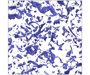
During the evolution, linear forcing is applied to regions of water to maintain $\varepsilon \approx 1$ (Rivière et al. 2021). Figure 4 shows the evolution of a sample simulation and figure 5 shows the evolution of the ensemble bubble-size distribution both for $We_T=100$. We note that, with our focus on bubbles $a>a_H$, the transition to a distinct a power-law regime for $N(a< a_H)$ is not captured (Deane & Stokes 2002). Over a measurement interval $t^n$ to $t^{n+1}=t^n+T$, ELA provides the unique, volume-conservative volume-tracking matrix, where each element $a_{ij}$ describes the volume that moved from a parent bubble $j$ that is identified at $t^n$ to a bubble $i$ identified at $t^{n+1}$ (Gaylo et al. 2022). From volume-tracking matrices, fragmentation statistics $\mathbb {E}\{\langle s \rangle _{T} \}$ and $p_{{\rm frag}}(a; T)$ can easily be computed. We study fragmentation statistics for parent bubbles of radii $a_0< a<1.2 a_0$, where $a_0=7 L/256$ provides a balance between the number of observed fragmentation events per simulation and resolution of the daughter bubbles. While this simulation is inherently transient, figure 5 illustrates that for this range of bubbles a quasisteady period exists. By initialising the bubbles to follow an equilibrium fragmentation cascade $N(a)\propto a^{-10/3}$ (Garrett et al. 2000), the fragmentation of bubbles $a>a_0$ maintains the population of bubbles $a\sim a_0$ for $t/t_\ell <3$, where $t_\ell ={(0.42)}^{-1} \varepsilon ^{-1/3} {a_0}^{2/3}$ is an a priori estimate of $\tau _\ell$ (Martínez-Bazán et al. 1999a). To exclude the fragmentation of the initial set of spherical bubbles (see figure 4), we study fragmentation over $1< t/t_\ell$. Thus, by measuring fragmentation statistics over $1< t/t_\ell <3$, we measure a quasisteady population of parent bubbles that are realistically formed by a fragmentation cascade.

Figure 4. Volume-of-fluid $f=0.5$ isosurface for one of the $We_T=100$ simulations at (a) $t/t_\ell =0$; (b) $t/t_\ell =1$; (c) $t/t_\ell =3$.

Figure 5. Average bubble-size distribution $N(a)$ for $We_T=100$ simulations at times: red, $t/t_\ell =0$; blue, $t/t_\ell =1$; green, $t/t_\ell =3$. Here $N(a)\propto a^{-10/3}$ is provided for reference over the range of initialised spherical bubbles (dashed line) and the range of measured parent bubbles, $a_0< a<1.2 a_0$ (solid line).

4.2. Grid independence

The choice of cell size, $\varDelta$, is driven by resolving the relevant scales of turbulence and surface tension. For turbulence, we compare the grid with the Kolmogorov microscale, $\eta \sim \varepsilon ^{-1/4} {\nu _w}^{3/4}$, where $\varDelta /\eta \lesssim 1$ ensures turbulence is resolved. For surface tension, we consider the cell Weber number $We_\varDelta = \rho _w u_{{rms}}^2 \varDelta /4 {\rm \pi}\sigma$, which estimates the ratio between the grid and the minimum characteristic radius of curvature of an interface deformed by inertial turbulence. Here $We_\varDelta <1$ ensures surface tension forces are resolved by the grid (Popinet 2018). We also consider $\varDelta /a_H$, comparing the grid to the Hinze scale: with $\varepsilon$ and $u_{{rms}}$ fixed ${We_\varDelta }^{3/5} \propto \varDelta /a_H$. Based on these metrics we find $L/\varDelta =256$ resolves turbulence and surface tension for our entire range of $We_T$ (see table 2).

With no clear lower limit to the ratio between the daughter-bubble and parent-bubble volume ($v^*$), grid resolution limitations require us to filter out daughter bubbles of radius $a<2 \varDelta$. Figure 6 shows that the bubble-size distribution of filtered bubbles, $N(a>2\varDelta )$, is grid-independent. For $L/\varDelta =256$ and parent bubbles $a_0=7 L/256$, $a<2 \varDelta$ corresponds to $v^*<0.02$. While this filter prevents us from measuring the full range of possible daughter bubbles, especially sub-Hinze daughters, we expect this to have little effect on the statistics of interest for two reasons. First, sub-Hinze bubble production by fragmentation happens concurrently with the production of large daughter bubbles (Rivière et al. 2022), so excluding small daughters should not affect the measured rate of fragmentation used to obtain $\tau _r$ and $\tau _\ell$. Second, for $\tau _c$, the integral of the daughter-size distribution in (3.17) weights local daughter production ($v^*\sim 1/\bar {m}$) over non-local daughter production ($v^*\ll 1$), making the contribution of the excluded small daughters small. This is related conceptually to locality, which suggests $v^*\ll 1$ can be neglected when modelling the cascade (Chan et al. 2021b,c).

Figure 6. Average bubble-size distribution $N(a>2\varDelta )$ for $We_T=200$ at time $t/t_\ell =3$ from simulations with grids: magenta, $L/\varDelta =128$; green, $L/\varDelta =192$; black, $L/\varDelta =256$; blue, $L/\varDelta =384$. Horizontal axis is normalised by $\varDelta =L/256$ and $N(a)\propto a^{-10/3}$ is provided for reference over the range of initialised spherical bubbles (dashed line) and the range of measured parent bubbles, $a_0< a<1.2 a_0$ (solid line).

To confirm that we resolve turbulence and surface tension, that the filter has a negligible effect, and (more broadly) that the statistics we measure are independent of the grid, we perform a convergence study for $We_T=200$ using three additional grids, $L/\varDelta =128$, $192$ and $384$. The results of this convergence study (see figure 7) show that our measurements of fragmentation statistics $\mathbb {E}\{\langle s \rangle _{T} \}$ and $p_{{\rm frag}}(a; T)$ (from which the time scales will be calculated) are grid independent for $L/\varDelta \ge 256$.

Figure 7. Grid-convergence study for (a) fragmentation rate constant $C_\varOmega$ and (b) convergence constant $C_\tau$ based on simulations of $We_T=200$ (parent bubbles $We=50$–$71$) with different grids, measured using $T/t_\ell =0.4$. Error bars indicate $95\,\%$ confidence interval.

4.3. Estimating relaxation time, $\tau _r$

For each simulation, we use six instances of ELA with different measurement intervals $T$. Using (2.4) and (2.7), we calculate $C_\varOmega (We; T)$ from each $p_{{frag}}(a;T)$. Figure 8(a) shows how $T$ affects the measured value of $C_\varOmega$, where we use $T/t_\ell =0.4$ as a reference value for each $We$. If the no-hysteresis assumption were valid for all $T$, $C_\varOmega$ would be a constant for each $We$. Figure 8(a), however, shows a strong dependence on small $T$. We observe that this dependence is approximately exponential, which provides an empirical definition of the relaxation time $\tau _r$ as well as the hysteresis strength $A$:

(4.1)\begin{equation} C_\varOmega(We; T)/C_\varOmega(We; T\sim\infty) = 1 + A \exp[{-}T/\tau_r] {.} \end{equation}

We observe that $\tau _r$ scales like $\tau _\ell$ rather than, say, bubble natural period, $We^{-1/2} \varepsilon ^{-1/3} a^{2/3}$. Thus, we define the scaling constant $C_r$ and write $\tau _r=C_r \varepsilon ^{-1/3} {a}^{2/3}$. This scaling suggests that, for $We>We_H$, the physical mechanisms for the decay of hysteresis are not related to surface tension. Future, more detailed, studies of the dynamics of individual bubbles are necessary to understand hysteresis and identify the mechanisms for its decay. For our statistical study, our concern is to determine when hysteresis can be neglected. Least-squares regression of the combined data for all $We$ gives $C_r\approx 0.11$. Hereafter, we measure all results with $T/t_\ell =0.4$ (corresponding to $T/\tau _r \approx 8$), which guarantees that effect of hysteresis on our estimation of $\tau _\ell$ and $\tau _c$ is negligible.

Figure 8. Measured (a) fragmentation-rate constant $C_\varOmega$ normalised by $(C_\varOmega )_{ref}$, the value measured using $T/t_\ell =0.4$ and (b) the convergence constant $C_\tau$ for $We$ of ($\circ$) $101$–$142$; ($\times$) $50$–$71$; ($\square$) $25$–$36$; ($\vartriangle$) $13$–$18$; ($\triangledown$) $6.3$–$8.9$. In (a), variance-weighted least-squares fit of all data to (4.1) (dashed line) gives $C_r=0.11$ and $A=2.2$ ($R^2=0.954$). In (b), error bars indicate $95\,\%$ confidence interval and the estimated large-$We$ value of $C_\tau =9$ (dashed line) is included for reference.

4.4. Estimating bubble lifetime, $\tau _\ell$

We now seek the expected bubble lifetime, $\tau _\ell$. Figure 9(a) shows our measurements of $C_\varOmega (We)$ and their fit to (2.5). We find the Hinze-scale $We_H=6.9$, similar to $We_H=4.7$ measured by Martínez-Bazán et al. (1999a) and $We_H=2.7\unicode{x2013}7.8$ by Risso & Fabre (1998). However, we obtain $C_{\varOmega,\infty }=1.4$, greater than $C_{\varOmega,\infty }=0.42$ measured by Martínez-Bazán et al. (1999a) and $C_{\varOmega,\infty }=0.95$ from HIT simulations by Rivière et al. (2021). An important distinction between our fragmentation rate measurements and previous experimental and numerical measurements is that we measure bubbles that have been formed as the daughters of previous fragmentation, so the bubbles are already distorted by fragmentation. The effect of this distinction can be demonstrated by measuring the fragmentation statistics over an earlier time in our simulation, $0< t/t_\ell <1$, when (as opposed to the later time $1< t/t_\ell <3$) many parent bubbles which started spherical have not yet fragmented. When we measure this earlier time range (denoted by $({\cdot })_{t< t_\ell }$), we obtain a similar $(We_H)_{t< t_\ell }=7.0$ but an appreciably smaller $(C_{\varOmega,\infty })_{t< t_\ell }=0.88$ ($R^2=0.974$). As our interest is bubbles within fragmentation cascades, our value of $C_{\varOmega,\infty }\approx 1.4$ is more relevant for bubbles formed by fragmentation. Note that $1/C_{\varOmega,\infty }$ is an order of magnitude larger than $C_r$ (i.e. $\tau _\ell \gg \tau _r$), which confirms that the PBE no-hysteresis assumption is reasonable when modelling fragmentation cascades.

Figure 9. (a) Fragmentation rate constant $C_\varOmega$ and (b) convergence constant $C_\tau$ as functions of $We$, measured using $T/t_\ell =0.4$. Error bars indicate $95\,\%$ confidence interval. In (a), variance-weighted least-squares fit to (2.5) (dashed line) gives $We_H=6.9$ and $C_{\varOmega,\infty }=1.4$ ($R^2=0.890$). In (b), the estimated large-$We$ value of $C_\tau =9$ (dashed line) is included for reference.

4.5. Estimating convergence time, $\tau _c$

We now seek the convergence time, $\tau _c$. As shown in § 3, the time-averaged speed $\mathbb {E}\{\langle s \rangle _{T} \}$, available from ELA, gives a $T$-independent measurement of $C_\tau$ so long as (3.18) is satisfied. Figure 9(b) shows the value of $C_\tau$ we obtain over a range of $We$. We find that the model developed in § 3, which as a result of large-$We$ assumptions predicts a constant $C_\tau$, is accurate for $We\gg We _H$, or more specifically $We>30$, where we measure $C_\tau \approx 9$. To validate that our measurement is $T$-independent, we also measure $C_\tau$ using a range of $T$ for $We=$ $50$–$71$ (figure 8b). As expected, for $T\lesssim \tau _r$ we see a dependence on $T$ due to hysteresis, but for $T\gg \tau _r$ $C_\tau$ is independent of $T$. Using $C_\tau = 9$, (3.18) gives $T/T_U<0.2$ for $We>30$, so we do not expect any effect of the Hinze scale driven upper bound on $T$-independence described in § 3.4.

5. Discussion

We now examine how the relaxation time $\tau _r$, bubble lifetime $\tau _\ell$ and convergence time $\tau _c$ inform the study of fragmentation. For $\tau _r$, our results suggest that the physical mechanism for the decay of hysteresis with bubble age is independent of surface tension for $We>We_H$ and that $\tau _r$ scales like $\tau _\ell$. The respective scaling constants we estimate from DNS of HIT differ by an order of magnitude ($C_r\ll 1/C_{\varOmega,\infty }$), suggesting that $\tau _r\ll \tau _\ell$ is always true for $We>We_H$. Although the physical mechanism for the decay of hysteresis is unclear, this shows that hysteresis can be assumed negligible when modelling fragmentation, validating an essential assumption of PBE. More practically, knowledge of $\tau _r$ also informs the choice of measurement interval in experiments and simulations. Here $T\gg \tau _r$ makes the effect of hysteresis on measurements negligible, ensuring that the measured fragmentation statistics are compatible with PBE.

The insight that the convergence time $\tau _c$ provides into the evolution of the bubble-size distribution in fragmentation-dominated bubbly flows has been discussed by Qi et al. (2020) and Deike et al. (2016), and we have now quantified $\tau _c$ directly. For large $We$ where the effect of surface tension on fragmentation rates is negligible, we find

(5.1)\begin{equation} \tau_c = C_\tau \varepsilon^{{-}1/3} {a_{max}}^{2/3} [1-(We_{max}/We_H)^{{-}2/5}] {,} \end{equation}

where $We_{max}$ is the Weber number of the largest bubble in the cascade (radius $a_{max}$) and we estimate $C_\tau \approx 9$ and $We_H\approx 6.9$ from DNS. In addition, as we can now express $\tau _c$ in terms of realistic fragmentation statistics for $We>30$, $\tau _c$ also informs large-$We$ fragmentation models. Inspired by (2.3), we rearrange (3.17) to provide a new bound on a moment of the daughter-size distribution $f_V^*$:

(5.2)\begin{equation} \bar{m} \int_0^1 {v^*}^{11/9} f_V^*(v^*) \,\mathrm{d} v^* = 1-(C_\tau C_{\varOmega,\infty})^{{-}1} {,} \end{equation}

where our estimations of $C_\tau \approx 9$ and $C_{\varOmega,\infty }=1.4$ from DNS give $0.92$ for the right-hand side of (5.2). For a physical interpretation, (2.3) bounds the relationship between daughter-size distributions and $\bar {m}$ to guarantee volume conservation, while (for $We>30$) (5.2) bounds the relationship to match the empirical value of $\tau _c$.

Many existing fragmentation models assume binary breakup ($\bar {m}=2$). To evaluate how well these meet (5.2), we focus on the proposed daughter-size distributions through $C_f$, which includes the integral in (5.2). With $\bar {m}=2$, $C_\tau \approx 9$ and $C_{\varOmega,\infty }=1.4$, we obtain $C_f\approx 1.8$. Because $C_f$ indicates how much longer $\tau _c$ is compared with the case of identical fragmentation, this shows that $\tau _c$ is $1.8$ times longer for fragmentation in HIT than what would be predicted if one assumes identical binary-fragmentation. Comparing with more realistic binary daughter-distributions (B–D in table 1), we see good agreement with the distribution proposed by Martínez-Bazán et al. (2010). We also compare with the binary daughter-distribution model by Qi et al. (2020, eq. (7)), which uses an experimentally constrained fitting parameter $\omega =0.3$ designed to tune the value of $\tau _c$. For their daughter-distribution model, (3.17) gives $C_f=1.741$, in good agreement with our value of $C_f\approx 1.8$. Although we assume $\bar {m}=2$ here for illustration, this analysis is applicable to any $\bar {m}$. Rather than attempting to compare the details of disparate fragmentation models, relating $\tau _c$ to the fragmentation statistics specified by these models allows us to directly compare the physical predictions each model makes regarding the evolution of the bubble-size distribution through a simple scalar quantity.

6. Conclusion

For air–water bubbly flows under HIT at moderate to large Weber numbers, we describe three fundamental time scales characterising the statistics of the evolution of the bubble-size distribution by fragmentation and the resulting fragmentation cascade. The prevalence of the observation of a $-10/3$ power-law in bubble-size distributions in bubbly flow for moderate and large $We$ demonstrates the importance of fragmentation cascades to the bubble-size distribution, and these time scales directly support statistical modelling of fragmentation. Although our focus here is on statistical descriptions of fragmentation, the results here also help inform mechanistic study of fragmentation.

One fundamental time scale is the relaxation time $\tau _r$ which characterises the time after fragmentation over which hysteresis cannot be neglected. From DNS measurements, we provide an empirical definition of $\tau _r$ based on when measured fragmentation rates become independent of the measurement interval $T$. We find that $\tau _r= C_r \varepsilon ^{-1/3} a^{2/3}$, where $C_r\approx 0.11$ independent of moderate/large $We$. This $We$-independence suggests the physical mechanism causing $\tau _r$ at these $We$ is unrelated to surface tension. Although understanding hysteresis and its decay is an area of future work, by providing $\tau _r$ we identify the time scales over which hysteresis can be neglected.

A second fundamental time scale is the expected lifetime $\tau _\ell$ of a bubble from formation by fragmentation to further fragmentation. For $\tau _\ell \gg \tau _r$, $\tau _\ell =[C_\varOmega (We)]^{-1}\varepsilon ^{-1/3} a^{2/3}$ is the inverse of the fragmentation rate. Fitting our DNS results for bubbles within the fragmentation cascade to the square-root model of $We$-dependence by Martínez-Bazán et al. (1999a) (2.5), we find the Hinze-scale $We_H\approx 6.9$, in agreement with previous experiments, but measure a smaller $\tau _\ell$ corresponding to a higher scaling constant (at large $We$) $C_{\varOmega,\infty }\approx 1.4$ (compared with $C_{\varOmega,\infty }\approx 0.42$ reported by Martínez-Bazán et al. (1999a)). We show that this higher value of $C_{\varOmega,\infty }$ is related to formation of the bubbles by a fragmentation cascade. For modelling fragmentation cascades, this higher $C_{\varOmega,\infty }$ is likely more relevant. In either case, we find $\tau _r\ll \tau _\ell$ for all $We$, validating the use of the no-hysteresis assumption in modelling fragmentation.

Finally, we consider the fundamental time scale $\tau _c= C_\tau [1-(We_{max}/ We_H)^{-2/5}] \varepsilon ^{-1/3} a_{max}^{2/3}$, which measures the time for a Lagrangian air particle to go from the largest bubble to the Hinze scale. This also characterises the time for fragmentation cascades to reach equilibrium. For large $We$, we derive $\tau _c$ based on the (constant) expected speed $\bar {s}$ at which a Lagrangian air particle moves through the cascade. We show that, $C_\tau =1/\bar {s}$ and can thus be measured independent of $T$. This result is valid for $\tau _r\ll T\ll \tau _c$, which provides a bound on the choice of $T$ in experiments and simulations. The $T$-independence of $C_\tau$ is confirmed by DNS measurements, which give $C_\tau \approx 9$ for $We>30$, which agrees well with the values obtained from the fragmentation model of Martínez-Bazán et al. (2010) and an experimentally constrained fragmentation model of Qi et al. (2020). The relationship between $C_\tau$ and fragmentation statistics in PBE provides new constraints on these statistics, at large $We$, limiting the possible forms of fragmentation models. Further, by quantifying $C_\tau$, we obtain the convergence time of fragmentation cascades $\tau _c$, beyond which a quasisteady model of fragmentation would be appropriate.

References

Campbell, B. 2014 A mechanistic investigation of nonlinear interfacial instabilities leading to slug formation in multiphase flows. PhD thesis, Massachusetts Institute of Technology, Cambridge, MA.Google Scholar
Castro, A.M. & Carrica, P.M. 2013 Bubble size distribution prediction for large-scale ship flows: model evaluation and numerical issues. Intl J. Multiphase Flow 57, 131150.CrossRefGoogle Scholar
Chan, W.H.R., Dodd, M.S., Johnson, P.L. & Moin, P. 2021 a Identifying and tracking bubbles and drops in simulations: a toolbox for obtaining sizes, lineages, and breakup and coalescence statistics. J. Comput. Phys. 432, 110156.CrossRefGoogle Scholar
Chan, W.H.R., Johnson, P.L. & Moin, P. 2021 b The turbulent bubble break-up cascade. Part 1. Theoretical developments. J. Fluid Mech. 912, A42.CrossRefGoogle Scholar
Chan, W.H.R., Johnson, P.L., Moin, P. & Urzay, J. 2021 c The turbulent bubble break-up cascade. Part 2. Numerical simulations of breaking waves. J. Fluid Mech. 912, A43.CrossRefGoogle Scholar
Deane, G.B. & Stokes, M.D. 2002 Scale dependence of bubble creation mechanisms in breaking waves. Nature 418, 839844.CrossRefGoogle ScholarPubMed
Deike, L. 2022 Mass transfer at the ocean–atmosphere interface: the role of wave breaking, droplets, and bubbles. Annu. Rev. Fluid Mech. 54 (1), 191224.CrossRefGoogle Scholar
Deike, L., Melville, W.K. & Popinet, S. 2016 Air entrainment and bubble statistics in breaking waves. J. Fluid Mech. 801, 91129.CrossRefGoogle Scholar
Diemer, R.B. & Olson, J.H. 2002 A moment methodology for coagulation and breakage problems. Part 3. Generalized daughter distribution functions. Chem. Engng Sci. 57, 41874198.CrossRefGoogle Scholar
Garrett, C., Li, M. & Farmer, D. 2000 The connection between bubble size spectra and energy dissipation rates in the upper ocean. J. Phys. Oceanogr. 30 (9), 21632171.2.0.CO;2>CrossRefGoogle Scholar
Gaylo, D.B., Hendrickson, K. & Yue, D.K.P. 2021 Effects of power-law entrainment on bubble fragmentation cascades. J. Fluid Mech. 917, R1.CrossRefGoogle Scholar
Gaylo, D.B., Hendrickson, K. & Yue, D.K.P. 2022 An Eulerian label advection method for conservative volume-based tracking of bubbles/droplets. J. Comput. Phys. 470, 111560.CrossRefGoogle Scholar
Hendrickson, K., Weymouth, G.D. & Yue, D.K.P. 2020 Informed component label algorithm for robust identification of connected components with volume-of-fluid method. Comput. Fluids 197, 104373.CrossRefGoogle Scholar
Hinze, J.O. 1955 Fundamentals of the hydrodynamic mechanism of splitting in dispersion processes. AIChE J. 1, 289295.CrossRefGoogle Scholar
Liao, Y. & Lucas, D. 2009 A literature review of theoretical models for drop and bubble breakup in turbulent dispersions. Chem. Engng Sci. 64, 33893406.CrossRefGoogle Scholar
Lundgren, T.S. 2003 Linearly forced isotropic turbulence. Tech. Rep. Center for Turbulence Research, Stanford University.Google Scholar
Martínez-Bazán, C., Montañés, J.L. & Lasheras, J.C. 1999 a On the breakup of an air bubble injected into a fully developed turbulent flow. Part 1. Breakup frequency. J. Fluid Mech. 401, 157182.CrossRefGoogle Scholar
Martínez-Bazán, C., Montañés, J.L. & Lasheras, J.C. 1999 b On the breakup of an air bubble injected into a fully developed turbulent flow. Part 2. Size pdf of the resulting daughter bubbles. J. Fluid Mech. 401, 183207.CrossRefGoogle Scholar
Martínez-Bazán, C., Rodríguez-Rodríguez, J., Deane, G.B., Montaes, J.L. & Lasheras, J.C. 2010 Considerations on bubble fragmentation models. J. Fluid Mech. 661, 159177.CrossRefGoogle Scholar
Popinet, S. 2009 An accurate adaptive solver for surface-tension-driven interfacial flows. J. Comput. Phys. 228 (16), 58385866.CrossRefGoogle Scholar
Popinet, S. 2018 Numerical models of surface tension. Annu. Rev. Fluid Mech. 50 (1), 4975.CrossRefGoogle Scholar
Qi, Y., Mohammad Masuk, A.U. & Ni, R. 2020 Towards a model of bubble breakup in turbulence through experimental constraints. Intl J. Multiphase Flow 132, 103397.CrossRefGoogle Scholar
Qi, Y., Tan, S., Corbitt, N., Urbanik, C., Salibindla, A.K.R. & Ni, R. 2022 Fragmentation in turbulence by small eddies. Nat. Commun. 13, 469.CrossRefGoogle ScholarPubMed
Risso, F. & Fabre, J. 1998 Oscillations and breakup of a bubble immersed in a turbulent field. J. Fluid Mech. 372, 323355.CrossRefGoogle Scholar
Rivière, A., Mostert, W., Perrard, S. & Deike, L. 2021 Sub-Hinze scale bubble production in turbulent bubble break-up. J. Fluid Mech. 917, A40.CrossRefGoogle Scholar
Rivière, A., Ruth, D.J., Mostert, W., Deike, L. & Perrard, S. 2022 Capillary driven fragmentation of large gas bubbles in turbulence. Phys. Rev. Fluids 7 (8), 083602.CrossRefGoogle Scholar
Rosales, C. & Meneveau, C. 2005 Linear forcing in numerical simulations of isotropic turbulence: physical space implementations and convergence properties. Phys. Fluids 17, 095106.CrossRefGoogle Scholar
Skartlien, R., Sollum, E. & Schumann, H. 2013 Droplet size distributions in turbulent emulsions: breakup criteria and surfactant effects from direct numerical simulations. J. Chem. Phys. 139, 174901.CrossRefGoogle ScholarPubMed
Solsvik, J., Maaß, S. & Jakobsen, H.A. 2016 Definition of the single drop breakup event. Ind. Engng Chem. Res 55, 28722882.CrossRefGoogle Scholar
Sporleder, F., Borka, Z., Solsvik, J. & Jakobsen, H.A. 2012 On the population balance equation. Rev. Chem. Engng 28, 149169.Google Scholar
Tsouris, C. & Tavlarides, L.L. 1994 Breakage and coalescence models for drops in turbulent dispersions. AIChE J. 40, 395406.CrossRefGoogle Scholar
Valentas, K.J., Bilous, O. & Amundson, N.R. 1966 Analysis of breakage in dispersed phase systems. Ind. Engng Chem. Fundam. 5, 271279.CrossRefGoogle Scholar
Vejražka, J., Zedníková, M. & Stanovský, P. 2018 Experiments on breakup of bubbles in a turbulent flow. AIChE J. 64, 740757.CrossRefGoogle Scholar
Weymouth, G.D. & Yue, D.K.P. 2010 Conservative volume-of-fluid method for free-surface simulations on Cartesian-grids. J. Comput. Phys. 229 (8), 28532865.CrossRefGoogle Scholar
Yu, X., Hendrickson, K., Campbell, B.K. & Yue, D.K.P. 2019 Numerical investigation of shear-flow free-surface turbulence and air entrainment at large Froude and Weber numbers. J. Fluid Mech. 880, 209238.CrossRefGoogle Scholar
Yu, X., Hendrickson, K. & Yue, D.K.P. 2020 Scale separation and dependence of entrainment bubble-size distribution in free-surface turbulence. J. Fluid Mech. 885, R2.CrossRefGoogle Scholar