


1. Corrected rate function
Note that the correct rate function also appears in the PhD thesis [Reference Stone3] (see Proposition 1.4.18), but with a different proof. We first give a slightly simplified proof of [Reference Jacquier, Pakkanen and Stone1, Theorem 3.1]. Any unexplained notation is as in [Reference Jacquier, Pakkanen and Stone1].
Let
 $Y:= \int_0^\cdot \varphi(u,\cdot)\,\mathrm{d} W_u$
be the Gaussian process from that theorem, and
$Y:= \int_0^\cdot \varphi(u,\cdot)\,\mathrm{d} W_u$
be the Gaussian process from that theorem, and
 $K_Y:\mathcal{C}^* \to \mathcal{C}$
its covariance operator (definition in [Reference Lifshits2, p. 5]). As noted in [Reference Jacquier, Pakkanen and Stone1],
$K_Y:\mathcal{C}^* \to \mathcal{C}$
its covariance operator (definition in [Reference Lifshits2, p. 5]). As noted in [Reference Jacquier, Pakkanen and Stone1],
 $\mathcal{I}^\varphi$
is injective by Titchmarsh’s convolution theorem. By the factorization theorem [Reference Lifshits2, Theorem 4.1] and the discussion in [Reference Lifshits2, pp. 32–33], it suffices to verify the factorization identity
$\mathcal{I}^\varphi$
is injective by Titchmarsh’s convolution theorem. By the factorization theorem [Reference Lifshits2, Theorem 4.1] and the discussion in [Reference Lifshits2, pp. 32–33], it suffices to verify the factorization identity
 $\mathcal{I}^\varphi(\mathcal{I}^\varphi)^*=K_Y$
to conclude that the reproducing kernel Hilbert space (RKHS) is the image
$\mathcal{I}^\varphi(\mathcal{I}^\varphi)^*=K_Y$
to conclude that the reproducing kernel Hilbert space (RKHS) is the image
 $\mathcal{I}^\varphi\big(L^2([0,1])\big)$
. By Fubini’s theorem, we have
$\mathcal{I}^\varphi\big(L^2([0,1])\big)$
. By Fubini’s theorem, we have
 $(\mathcal{I}^\varphi)^* \mu = \int_\cdot^1 \varphi(\cdot,t)\mu(\mathrm{d} t)$
for any measure
$(\mathcal{I}^\varphi)^* \mu = \int_\cdot^1 \varphi(\cdot,t)\mu(\mathrm{d} t)$
for any measure
 $\mu \in \mathcal{C}^*$
. We then compute, for
$\mu \in \mathcal{C}^*$
. We then compute, for
 $\mu,\nu \in \mathcal{C}^*$
,
$\mu,\nu \in \mathcal{C}^*$
,
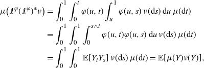 \begin{align*} \mu\big(\mathcal{I}^\varphi(\mathcal{I}^\varphi)^* \nu\big) &= \int_0^1 \int_0^t \varphi(u,t) \int_u^1 \varphi(u,s)\, \nu(\mathrm{d} s)\, \mathrm{d} u\, \mu(\mathrm{d} t) \\[2pt] &= \int_0^1 \int_0^1 \int_0^{s \wedge t} \varphi(u,t) \varphi(u,s)\, \mathrm{d} u\, \nu(\mathrm{d} s)\, \mu(\mathrm{d} t) \\[2pt] &= \int_0^1 \int_0^1 \mathbb{E}[Y_t Y_s]\, \nu(\mathrm{d} s)\, \mu(\mathrm{d} t) = \mathbb{E}[ \mu(Y) \nu (Y)],\end{align*}
which proves the theorem.
The second definition in [Reference Jacquier, Pakkanen and Stone1, (2.3)] should be replaced by the following one.
Definition 1. For
 $\Phi:\mathbb{R}^+ \times \mathbb{R}^+ \to \mathbb{R}^{2\times2},$
define
$\Phi:\mathbb{R}^+ \times \mathbb{R}^+ \to \mathbb{R}^{2\times2},$
define
 $\mathcal{I}^{\Phi}:L^2([0,1],\mathbb{R}^2) \to L^2([0,1],\mathbb{R}^2)$
by
$\mathcal{I}^{\Phi}:L^2([0,1],\mathbb{R}^2) \to L^2([0,1],\mathbb{R}^2)$
by
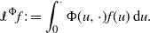 \begin{equation*} \mathcal{I}^{\Phi} f := \int_0^\cdot \Phi(u,\cdot)f(u) \, \mathrm{d} u. \end{equation*}
The following theorem replaces [Reference Jacquier, Pakkanen and Stone1, Theorem 3.2].
Theorem 1. Let
 $\varphi_1,\varphi_2$
satisfy [Reference Jacquier, Pakkanen and Stone1, Assumption 3.1], and define
$\varphi_1,\varphi_2$
satisfy [Reference Jacquier, Pakkanen and Stone1, Assumption 3.1], and define
 $Y_i:= \int_0^\cdot \varphi_i(u,\cdot) \, \mathrm{d} W_u^i$
,
$Y_i:= \int_0^\cdot \varphi_i(u,\cdot) \, \mathrm{d} W_u^i$
,
 $i=1,2$
, where
$i=1,2$
, where
 $W^1$
and
$W^1$
and
 $W^2$
are standard Brownian motions with correlation parameter
$W^2$
are standard Brownian motions with correlation parameter
 $\rho \in(-1,1)$
. Then, the RKHS of
$\rho \in(-1,1)$
. Then, the RKHS of
 $(Y_1,Y_2)$
is
$(Y_1,Y_2)$
is
 $\mathcal{H}^\Phi := \{ \mathcal{I}^\Phi f : f \in L^2([0,1],\mathbb{R}^2) \}$
, with inner product
$\mathcal{H}^\Phi := \{ \mathcal{I}^\Phi f : f \in L^2([0,1],\mathbb{R}^2) \}$
, with inner product
 $\langle \mathcal{I}^\Phi f, \mathcal{I}^\Phi g \rangle = \langle f,g \rangle$
, where
$\langle \mathcal{I}^\Phi f, \mathcal{I}^\Phi g \rangle = \langle f,g \rangle$
, where
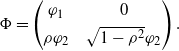 \begin{equation*} \Phi = \begin{pmatrix} \varphi_1 &\quad 0 \\[3pt] \rho \varphi_2 &\quad \sqrt{1-\rho^2}\varphi_2 \end{pmatrix}. \end{equation*}
Proof. Analogous to the proof above. Injectiveness of
 $\mathcal{I}^\Phi$
follows from the Titchmarsh convolution theorem. We have
$\mathcal{I}^\Phi$
follows from the Titchmarsh convolution theorem. We have
 $(\mathcal{I}^\Phi)^*\mu = \int_\cdot^1 \Phi^{\top}(\cdot,t) \mu(\mathrm{d} t)$
for any measure
$(\mathcal{I}^\Phi)^*\mu = \int_\cdot^1 \Phi^{\top}(\cdot,t) \mu(\mathrm{d} t)$
for any measure
 $\mu\in(\mathcal{C}^2)^*$
. The factorization identity
$\mu\in(\mathcal{C}^2)^*$
. The factorization identity
 $\mathcal{I}^\Phi(\mathcal{I}^\Phi)^*=K_{Y_1,Y_2}$
is verified as above.
$\mathcal{I}^\Phi(\mathcal{I}^\Phi)^*=K_{Y_1,Y_2}$
is verified as above.
Theorem 1 implies the following corollary, which replaces [Reference Jacquier, Pakkanen and Stone1, Corollary 3.2].
Corollary 1. The RKHS of the measure induced on
 $\mathcal{C}^2$
by the process (Z,B) is
$\mathcal{C}^2$
by the process (Z,B) is
 $\mathcal{H}^{\Psi}$
, where
$\mathcal{H}^{\Psi}$
, where
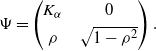 \begin{equation*} \Psi = \begin{pmatrix} K_\alpha &\quad 0 \\[3pt] \rho &\quad \sqrt{1-\rho^2} \end{pmatrix}. \end{equation*}
Consequently,
 $\| \cdot \|_{\mathcal{H}^{\Psi}}$
should replace
$\| \cdot \|_{\mathcal{H}^{\Psi}}$
should replace
 $\| \cdot \|_{\mathcal{H}_\rho^{K_\alpha}}$
in line 4 of p. 1083 and in the proof of [Reference Jacquier, Pakkanen and Stone1, Theorem 2.1] on p. 1088. The special case
$\| \cdot \|_{\mathcal{H}_\rho^{K_\alpha}}$
in line 4 of p. 1083 and in the proof of [Reference Jacquier, Pakkanen and Stone1, Theorem 2.1] on p. 1088. The special case
 $\rho=0$
requires no separate treatment, and the result agrees with [Reference Jacquier, Pakkanen and Stone1, Section 5].
$\rho=0$
requires no separate treatment, and the result agrees with [Reference Jacquier, Pakkanen and Stone1, Section 5].
2. Minor corrections
-
1. On p. 1079, last line of the introduction: replace
 $\int_0^1$
by
$\int_0^\cdot$
.
$\int_0^1$
by
$\int_0^\cdot$
. -
2. On p. 1084, definition of topological dual: add ‘continuous’ before ‘linear functionals’.
-
3. On p. 1085, second displayed formula: after the second
$=$
, replace f by
$\Gamma(f^*)$
. -
4. In the statement of Theorem 3.4,
$\varepsilon \mu$
should be replaced by
$\mu(\varepsilon^{-1/2}\,\cdot)$
. The speed
$\varepsilon^{-\beta}$
resulting from the application of the theorem on p. 1088 is correct, though. -
5. First line of p. 1089: Replace
$v_0^{1+\beta}$
by
$v_0 \varepsilon^{1+\beta}$
. To make the estimate work for
$t=0$
, confine
$\varepsilon$
to the finite interval [0,1] instead of
$\mathbb{R}^+$
in line
${-4}$
of p. 1088.


