Ultrahigh frequency path loss prediction based on K-nearest neighbors

Abstract

Path loss prediction (PLP) is an important feature of wireless communications because it allows a receiver to anticipate the signal strength that will be received from a transmitter at a given distance. The PLP is done by using machine learning models that take into account numerous aspects such as the frequency of the signal, the surroundings, and the type of antenna. Various machine learning methods are used to anticipate path loss propagation but it is difficult to predict path loss in unknown propagation conditions. In existing models rely on incomplete or outdated data, which can affect the accuracy and reliability of predictions and they do not take into account the effects of environmental factors, such as terrain, foliage, and weather conditions, on path loss. Furthermore, existing models are not robust enough to handle the real-world variability and uncertainty, leading to significant errors in predictions. To tackle this issue, a novel ultrahigh frequency (UHF) PLP based on K-nearest neighbors (KNNs) is developed for predicting and optimizing the path loss for UHF. In this proposed model, a KNN-based PLP has been used to predict the path loss in the UHF. This technique is used for high-accuracy PLP through KNN forecast route loss by determining the K-nearest data points to a particular test point based on a distance metric. Moreover, the existing models were not able to optimize path loss due to complex and large-scale machine learning models. Therefore, the stochastic gradient descent technique has been used to minimize the objective function, which is often a measure of the difference between the model’s predictions and the actual output that will fine-tune the parameters of the KNN model, by measuring the similarity between data points. This model is implemented using Python to make it a lot more convenient.

Introduction

Mobile communication is regarded as one of our vital demands in the contemporary technological era. Due to the tremendous increase in communication devices, this generation will need services with a large amount of bandwidth and resources. The rapid evolution of communication technology from 2G toward 4G and 5G [1]. The goals of fifth-generation (5G) networks are increased throughput, wide coverage, reduced radio latency, enhanced spectral efficiency, and better connection density. Internet of things (IoT) applications will require wide coverage areas and diverse terrains. Broad bandwidths will also be provided via new frequency bands, like the millimeter-wave and sub-6 GHz bands. Several measurement sessions and drive tests will be necessary to obtain attenuation data at the new frequencies. In network planning for 5G mobile communication systems, appropriate models will need to be used in order to assess path loss. Path loss prediction (PLP) models have traditionally been created using deterministic or empirical methods [2].

The service providers are working hard to meet user expectations and deliver dependable communication. By extending the long-term evolution (LTE) networks to offer greater bandwidth, throughput, and improved service quality, it will be possible to implement these solutions and meet the criteria of the 5G networks. In terms of services, infrastructure, reconfiguration, and a wide range of operations, 5G networks will offer a greater mobile experience [3]. Machine learning makes use of big datasets and adaptable model architecture to provide predictions. Machine learning-based methods have been used recently in computer vision, data mining, speech recognition, and self-driving automobiles, among other fields. For these tasks, both supervised and unsupervised learning are applicable. Supervised learning with labelled data seeks to learn a precise and wide function between inputs and outputs in order to address problems related to regression and classification. On the other hand, unsupervised learning algorithms using unlabeled data must characterize the hidden structure. The PLP problem and decision tree are essentially resolved by supervised machine learning methods such as artificial neural networks (ANNs) and support vector regression (SVR). It has been stated that models based on machine learning are more computationally efficient than deterministic models and more accurate than empirical models [4–6].

The neural network maps a set of input values to a set of output values through a nonlinear process using layers of neurons. To do this, the input values are added to the appropriate synaptic weights for each layer, resulting in the correct output [7]. A function with several inputs and a single output is obtained to handle the PLP problem between two places. Information on the transmitter and receiver’s locations, the frequency, and adjacent structures are among the inputs [8]. Therefore, in order to provide the necessary output with topological and morphological knowledge about the environment value, the transformation of an input vector is employed to explain the prediction of path loss [9]. Furthermore, most of the research that has been published to date uses empirical models such as the log-distance and free-space models, which are based on data collected under certain propagation conditions. Statistical analysis is needed to build the mapping link between path loss and variables like aircraft height and propagation distance. Using aerial photos, a territory can also be classified as a forest or a village, for example, and the appropriate route loss model can be used to forecast path loss for sites other than urban areas [10].

Machine learning approaches are used to tackle supervised regression problems, such as PLP. According to recent research, machine learning-based route loss models predict path loss more accurately than empirical models and are even more computationally efficient than deterministic ones [11]. In order to analyze urban cellular propagation (RX), the physical environment between a transmitter (TX) and receiver must be classified as either line of sight (LOS) or non-line of sight (NLOS). A generalized path loss model is derived by modifying the free space path loss model with a path loss exponent (PLE) that changes with the environment, despite the low likelihood of free space propagation. In order to effectively predict PLP, NLOS environments are further divided into moderately and heavily obstructed environments. The moderately obstructed conditions have small obstructions, such as building edges or trees, that partially block the optical path between the TX and RX, while the heavily obstructed conditions have large obstructions that completely block the optical path [12, 13]. For PLP, additional machine learning techniques were also used, including decision trees and K-nearest neighbors (KNNs).

The KNN method is introduced into ultrahigh frequency (UHF) PLP for several reasons. KNN is a straightforward algorithm based on the idea that similar things are close to each other. In the context of UHF PLP, it’s intuitive to consider that similar distances, frequencies, or environmental factors might lead to similar path loss. UHF PLP often involves complex relationships between various factors such as distance, frequency, terrain, and obstacles. It is a nonparametric method, meaning it doesn’t make strong assumptions about the underlying data distribution. It can capture complex relationships and nonlinearities in the data without imposing a specific functional form. In wireless communication scenarios like UHF, the environment can change dynamically due to factors like moving objects or changing weather conditions. In addition, KNN, being an instance-based learning method, can adapt to changes in the environment since it doesn’t explicitly create a model; instead, it memorizes the training instances and uses them for prediction [14].

Moreover, KNN can serve as an initial exploration into UHF PLP. It can be used as a baseline model to understand the relationships between different parameters and the target variable. It allows for quick prototyping and understanding of the data before more complex models are explored. Furthermore, KNN tends to perform well when there’s sufficient data available, especially in cases where the decision boundary is irregular or complex. In UHF PLP, where multiple variables might influence the outcome, KNN’s ability to consider multiple features simultaneously can be advantageous [15]. However, UHF signals experience various propagation challenges due to their higher frequency range, including greater susceptibility to obstacles, reflections, and environmental factors. Accurate prediction of path loss is crucial for optimizing communication systems in these conditions. Overall, the introduction of KNN into UHF PLP provides a starting point that allows for exploring data relationships, providing intuitive insights, and potentially yielding reasonably accurate predictions. The main contribution of this paper is as follows:

• • To enhance and identify the path loss in the UHF wireless network in a complex environment, the UHF PLP based on KNNs is used.

• • To predict the propagation path loss for unknown propagation situations for UHF the proposed model uses K-nearest neighbor-based path loss prediction (KNN-PLP).

• • For wireless network optimization in the proposed model, an optimization algorithm named stochastic gradient descent (SGD) is used to optimize the UHF wireless network.

The content of the paper is structured as follows: literature survey, following that the technique and the novel solution, and results and discussion; finally concludes the paper.

Literature survey

Thrane et al. [8] proposed a model to evaluate mobile communication system performance and optimize coverage for existing deployments. Accurate radio performance estimation faces new issues due to the different 5G transmission frequencies. Traditional channel models are replaced by a channel model created using deep learning (DL) methods with the help of satellite pictures and a straightforward path loss model. Predictive performance has increased using model-aided DL. The proposed DL model is capable of increasing PLP at unseen places for 811 MHz with 1 dB and 4.7 dB for 2630 MHz. The model-aided approach delivers an improvement of 1 dB. However, it is difficult to obtain enough data to train a model that accurately predicts path loss in different environments.

Wen et al. [16] proposed a PLP model for an MD-82 aircraft cabin. The PLP model is constructed using machine learning techniques such as back-propagation neural network (BPNN), SVR, random forest, and AdaBoost. Based on knowledge already accessible at known frequencies, further study is conducted to anticipate route loss at a new frequency. Additionally, provide a PLP scheme combining empirical models and machine learning-based models to address the issue of data limitation at the new frequency. To increase the training set, this method leverages estimated values produced by the empirical model by earlier data. The training set for the route loss prediction at 5.8 GHz is composed of samples obtained from the empirical model and observed samples at 2.4 GHz and 3.52 GHz, respectively. If data availability is limited, it is difficult to obtain enough data to train a model to accurately predict path loss in different aircraft cabin environments.

Zyner et al. [17] presented a multimodal, probabilistic approach for driver intention and path prediction. Recurrent neural networks are used in conjunction with a mixture density network output function to accomplish this. A clustering technique is applied to this data, yielding a ranked list of unknown potential pathways. To corroborate the findings, a naturalistic dataset from real-world scenarios was collected, which included over 23,000 automobiles passing around five distinct roundabouts. This is the largest publicly available dataset of its kind, as far as the author is aware. A total of 5952 real-world trajectories were used to evaluate the method, and it performed better than all baselines. However, this method is computationally expensive, which could be a problem for real-time applications in which low latency predictions are required.

Faruk et al. [18] proposed a PLP model within urban environments. Effective planning and implementation of radio access networks in urban contexts require a thorough understanding of how radio waves behave in a real wireless channel. Although popular due to their simplicity, empirical propagation models are prone to significant prediction errors. The evaluation and analysis of signal fading forecasts in the very high frequency and UHF bands in typical metropolitan situations. Based on ANN, adaptive neuro-fuzzy inference system, and Kriging techniques, path loss models are created using the gathered data. The outcomes of the created models’ predictions are contrasted with those of a few empirical models and field measurements. Other than Egli and ECC-33, all other models’ root mean square errors (RMSEs) under investigation are considered acceptable. However, it is difficult to predict accurately in complex environments, such as urban areas with many buildings and other structures that cause signal reflections and absorption. This leads to large variations in signal strength, making it difficult to predict path loss accurately.

Abolade et al. [19] propose a new support vector machine (SVM)-based radio propagation model for path loss (PL)forecasts in urban settings. Field measurement campaigns are carried out in metropolitan settings to collect data on route loss and mobile network characteristics of radio signals broadcast at frequencies of 900, 1800, and 2100 MHz. In order to forecast path loss in an urban propagation context, an SVM model is trained using field measurement data. The mean absolute error (MAE), mean square error (MSE), RMSE, and standard error deviation (SED) are used to assess the performance of the SVM model. Additionally, the complexity of the proposed model makes it difficult to interpret and understand the model’s predictions, which could make it hard to identify and address any issues that arise during the prediction process.

Ahmadien et al.’s [10] any wireless communication system’s network planning is utterly dependent on PLP. For cellular networks, it is often accomplished through in-depth assessments of the target area’s received signal power. Ray tracing simulations are used when a 3D model of the area is available; however, a significant disadvantage of this strategy is the high computing complexity of the simulations. In this study, a deep convolutional neural network (CNN)-based method for predicting the path loss distribution directly from 2D satellite pictures. The inference is performed in real-time, whereas the training procedure takes time and must be done offline. The 3D representation of the area is not required for inference using the suggested method because the network just utilizes an image captured by an aerial vehicle or satellite as its input. However, it requires satellite images to predict the path loss distribution, and 2D images are not sufficient to characterize the 3D structure in some cases. This is more critical for urban regions, especially when the transmitter altitude is low and the frequency is high.

Moraitis et al. [20] used a machine learning approach, to develop prediction path loss models for cellular networks in an urban context. A path loss dataset produced by simulated outcomes taking into account an LTE network using a digital terrain model is used to carry out the training and testing process. When simulating both LOS and NLOS propagation conditions, an urban environment is taken into account. The findings show that all of the methods under consideration forecast route loss with impressive accuracy, with RMSEs of 2.1–2.2 dB for LOS locations and 3.4–4.1 dB for NLOS locations, respectively. The KNN exhibits the best performance among the algorithms under consideration, making it a desirable alternative for PLP in metropolitan environments.

Ojo et al.’s [21] PLP models play an important role in wireless signal propagation due to the ongoing need to provide dependable and high-quality service to subscribers. Deterministic models are more accurate, but they are more difficult to develop, take more time, and have no adaptable characteristics. To that end, this paper proposes to address the issues with existing models by applying machine learning algorithms to PLPs. The data were collected in six base transceiver stations via drive test in multitransmitter scenarios, and the path loss of the received signal level was calculated and analyzed. The measured data was then used to create two machine learning-based PLP models. However, RBF neural networks can be computationally intensive and require a large amount of processing power, making them less suited for real-time implementation in resource-constrained environments.

Sotiroudis et al.’s [22] PLPs in metropolitan settings have been carried out using tabular data and photos as two distinct sorts of inputs from machine learning models. On these various sources of input information, many sorts of models are applied. The current work attempts to combine both types of input data into a single prediction model. Each feature of the tabular data vector is divided into several pixels according to its estimated relevance. The resulting synthetic images are then combined with pictures of particular parts of the local map. A CNN is then utilized as an input for compound pseudo images, which have channels of both map-based and tabular data-based images, to forecast the path loss value at a given distance. This approach could be applied for PLP in urban environments for several state-of-art wireless networks like 5G and the IoT. The presented framework is general and incorporates changes and/or additions within the tabular data or the images that constitute its channels.

Lee et al. [23] proposed a new algorithm for predicting the PLE of outdoor millimeter-wave band channels through a DL method. The wireless channel data was generated using a three-dimensional radio ray tracing tool to train the PLE on the neural network. The neural network’s performance in making predictions for the test data set was assessed after it had been trained using channel data collected from diverse contexts. It is possible to determine the ideal hyper parameter for predicting the PLE. Regarding the number of structures in the area or their typical distance from the transmitter, the forecast performance does not demonstrate any appreciable variation. However, the prediction is not accurate in all environments. Millimeter-wave channels are affected by various factors such as atmospheric absorption, vegetation, and buildings which vary greatly between different environments.

From the analysis, it is clear that paper [8] provides errors in predicting different environments, for paper [16] data availability is limited in aircraft cabin environments. In paper [17] is computationally expensive, for paper [18] it is difficult to predict in a complex environment. In paper [19] it is hard to identify and address issues during the prediction process. Paper [10] is more critical for the urban region. In paper [20] using KNN produces better prediction results. It takes a large amount of computation power and makes them not suitable for a complex environment [21]. Paper [22] incorporate changes within the tabular data. Millimeter-wave channels are affected by various factors [23]. Hence to fill this research gaps a novelty must be developed.

UHF PLP based on KNNs

PLP is important for UHF bands because it helps to understand the propagation of radio waves in a given environment. This information is crucial for the design, deployment, and optimization of wireless communication systems operating in the UHF band. There are various machine algorithms are used to predict the propagation of path loss and it is difficult to achieve for unknown propagation situations, which is not an ideal outcome. To tackle this issue, a novel UHF PLP based on KNNs has been developed to identify path loss in UHF with high frequency in any environment. For predicting the path loss, the KNN-PLP is utilized in the proposed model which makes KNN-PLP in the UHF network by identifying the K-nearest data points to a given test point based on a distance metric and forecast route loss to ensure high-accuracy prediction even in the complex environment. Moreover, using the KNN model results in overfitting when the model is too complex and starts to fit the noise or random fluctuations in the training data, rather than the underlying patterns. To overcome this difficulty, an SGD optimization has been used to reduce the overfitting problem and reduce the objective function, a measure of the discrepancy between the model’s output forecasts and reality that is frequently used to optimize the UHF wireless network. Hence, the proposed model is used to predict and optimize the UHF network with high accuracy.

Figure 1illustrates the process flow of the proposed model UHF-based PLP based on KNNs. The process begins with the collection of data in a 455 MHz UHF network, the various parameters such as distance, signal strength, and other relevant factors which affect path loss are collected. The data is then preprocessed, which includes feature extraction and scaling, to ensure that the data is in the appropriate format for the proposed model. Once the data is preprocessed, the proposed model uses KNN applied to determine the KNNs for each data point. The algorithm then uses the KNNs to predict the path loss for each data point by forecasting route loss. This process is repeated for all data points, and the final prediction is made based on the average of all the predictions. However, other factors affect the path loss in a wireless network so the proposed model uses an optimization algorithm to reduce path loss in the proposed model. The SGD optimization algorithm is used in the proposed model to reduce the overfitting problem. The proposed PLP model allows an accurate prediction and optimization even in complex wireless network environments.

Figure 1. Process flow of the proposed model.

K-nearest neighbor-based path loss prediction

To predict path loss in the wireless network, the proposed model UHF PLP based on KNNs has been presented to identify the path loss by using KNN. The ability to make predictions based on the information gathered from the nearest neighboring data points, especially in the UHF band, KNN is a type of instance-based learning algorithm, which means that it uses the data points closest to a new data point to make a prediction. The key idea behind the KNN-PLP model is to predict path loss at certain locations and efficiently predict path loss in unknown locations.

The proposed model initially collects a large amount of data on a 455 MHz UHF wireless network based on the factors that affect path loss. Preprocessing is applied to the collected data before it is used in the proposed model. The process of data preprocessing includes data cleaning, which involves removing and correcting any inaccurate data. Once the data is cleaned, it needs to be scaled to ensure that all the features are on the same scale. This is an important process in the proposed model because it works based on distance measures, and if the features are on different scales, the distance calculated is pointless. The min-max scaling is used in which all input features and path loss values are changed in the range from −1 to 1 or from 0 to 1. In a PLP model, feature extraction is identifying and extracting relevant information from the collected data that can be used to make predictions. This information is typically in the form of numerical or categorical variables, also known as features. These features are used as inputs to the prediction model. In the proposed PLP model for UHF, the data collection process involves measuring the signal strength at different locations and under different conditions. The extracted features include the distance between the transmitter and receiver, the transmitter and receiver’s height, the environment type, and obstacles such as buildings and trees. The distance-based feature extraction, such as Euclidian distance, is used in the proposed model and from feature-extracted datasets. The data is divided into a training set and a test set. The training set is used to train the KNN model, while the test set is used to evaluate its performance. In path loss models, KNN is used for prediction. KNN employs a weighted average of the KNNs, with the weight determined by the inverse of their distance. The KNN predicts the values of new data points based on feature similarity. This means that a value is assigned to the new point based on how closely it resembles the points in the training set.

Algorithm 1. Process flow of K-nearest neighbor-based path loss prediction (KNN-PLP)

Step 1: Data Collection and Preprocessing

# Assume you have a dataset with features (distances, signal strengths) and path loss values

# Data cleaning, normalization, and splitting into training and testing sets

Step 2: Choose K and Distance Metric

K = 5 # Set the number of neighbors

distance_metric = ‘euclidean’ # Choose distance metric (e.g., Euclidean distance)

Step 3: Training Phase

# In KNN, training involves storing the dataset (no explicit training step)

training_data = load_training_data() # Load the training dataset with path loss values

Step 4: Prediction Phase

def predict_path_loss(test_point):

distances = []

for data_point in training_data:

# Calculate distance between test point and each training data point

dist = calculate_distance(test_point, data_point, distance_metric)

distances.append((data_point, dist))

# Sort distances and select K nearest neighbors

distances.sort(key=lambda x: x[1])

nearest_neighbors = distances[:K]

# Calculate predicted path loss based on the average of K nearest neighbors’ path loss values

predicted_path_loss = sum(neighbor[0].path_loss for neighbor in nearest_neighbors)/K

return predicted_path_loss

Step 5: Evaluation

testing_data = load_testing_data() # Load the testing dataset

predictions = []

actual_values = []

for test_sample in testing_data:

predicted = predict_path_loss(test_sample)

actual = test_sample.path_loss

predictions.append(predicted)

actual_values.append(actual)

# Calculate evaluation metrics (e.g., RMSE, MSE, R-squared)

evaluation_metrics = calculate_metrics(predictions, actual_values)

Step 6: Model Refinement and Optimization

# Tune hyperparameters (K, distance metrics), feature engineering, cross-validation, etc.

Step 7: Deployment and Usage

# Use the trained model for path loss prediction in real-world scenarios

Algorithm 1 shows the process flow of KNN-PLP in the prediction of PLP. The extracted features data are used to ensure the data is in the appropriate format for KNN. The KNN algorithm is applied to the data to determine the KNNs for each data point. Then the KNN predicts the path loss in the network. The KNN model works by finding the KNNs of a new point based on its features. The path loss value at the new point is then predicted as the average of the path loss values of its KNNs. Nearest-neighbor methods in input space $x$ to form $C$ the KNN for $C$ are given in equation (1):

(1)\begin{equation}C\left( x \right) = \,\frac{1}{k}\mathop \sum \limits_{{x_i}} \in {N_k}\left( x \right){C_i}\,\,\,\,\,\,\end{equation}

where ${N_k}\left( x \right)$ is the neighbor of $x$ defined by the $k$ closest point ${x_i}$ in the model and the Euclidean distance is assumed to find the $k$ observation with ${x_i}$ closest to $x$ in input space and average responses. The Euclidian distance $E$ is calculated as the square root of the sum of the squared differences between points given in equation (2):

(2)\begin{equation}E = \sqrt {\mathop \sum \limits_{i = 1}^k {{\left( {{x_i} - {y_i}} \right)}^2}}. \,\,\,\,\,\,\end{equation}

When the values of $x$ and $y$ are the same, the distance $D$ to be equal to $0$, otherwise $D = 1$. The closest $k$ data points are selected based on the distance. The number of neighbors assigns a value to any new observation, and the average of these data points is the final prediction for the new one. The Euclidean distance is used in model training to determine the distance between each training point and the new point. Based on the determined distance, the closest $k$ data points are chosen, and the number of nearest neighbors gives any new observation a value. The outcome frequently varies depending on the $k$ value. The error calculation for the train and validation sets was used to optimize $k$. The training sample’s error rate at $k\, = \,1$ is always zero. The training data point is closest to itself. As a result, when $\,k\, = \,1$, the prediction is always correct. If the validation error curve resembles another, $k\, = \,1\,$ is selected. The validation error curve with different values of $k$ is mentioned in equation (2). It is overfitting the limits at $k\, = \,1$. As a result, the error rate initially declines and drops to a very low level. After the lowest point, it grows as it is raised. The training and validation are separated from the initial dataset to obtain the ideal value. After that, plot the validation error curve to get the optimal value. This value should be used for all predictions. The optimization algorithms, such as SGD are used in the proposed model as a first-order optimization algorithm that updates the model parameters iteratively by following the negative gradient of the loss function to the parameters.

Stochastic gradient descent

To optimize the UHF wireless network, the proposed model uses the SGD algorithm for finding the minimum of an objective function, which is a scalar function of one or more variables, by iteratively moving in the direction of the negative gradient of the function. SGD is considered the best optimization algorithm for the KNN-PLP model because of its ability to optimize non-convex functions, which is the case for PLP. The process flow of the SGD is shown in algorithm. Initially, the values of the weights and biased of the proposed model are arranged in random order for each iteration and evaluate the difference between the predicted and actual values for the PLP. How well the model fits the training data is indicated by the loss function, which is also known as the cost function. The cost function should be viewed with caution to improve model fit. The random point in the function is represented by the row vector$\,\upsilon $:

(3)\begin{equation}\upsilon = \left[ {{a_0},{a_1}, \ldots ,{a_n}} \right].\end{equation}

The cost function is evaluated by the difference between the predicted and actual values for the path loss in the training set given in equation (4):

(4)\begin{equation}Q\left( \upsilon \right) = \frac{1}{n}\mathop \sum \limits_{i = 1}^n {Q_i}\left( \upsilon \right){\text{ }}.\end{equation}

From equations (2–4), the ${Q_i}\left( \upsilon \right)$ is the value of the loss function at the ${i{\rm{th}}}$ data point and finding the minimized loss function.

(5)\begin{equation}Q\left( \upsilon \right) = \mathop \sum \limits_{i = 1}^n {\left( {{x_i} - {y_i}} \right)^2}\,\,\,\,\,\end{equation}

(6)\begin{equation}Q\left( \upsilon \right) = \mathop \sum \limits_{i = 1}^n {\left( {{a_1} + {a_2}{x_i} - {y_i}} \right)^2}\,\,\,\,\,\,\end{equation}

In equation (6), the $Q\left( \upsilon \right)$ is minimized objective function. The gradient is only evaluated at a random point. Whenever the gradient is being evaluated, it is necessary to pay for expensive evaluations of the gradients from all loss functions. When there are no simple formulas and the training set is very large, it becomes exceedingly expensive to evaluate the sums of gradients because doing so requires evaluating the gradients of all the loss functions. This is very effective in the case of large-scale machine learning problems. The parameters are updated using the gradient computed in the previous step and a learning rate, which determines the step size of the path loss optimization, and this process is repeated until the cost function converges or a maximum number of iterations is reached.

The SGD algorithm performs much better in large-scale datasets. The idea behind the algorithm is to find an efficient way of reaching the minimum value of a function. The SGD algorithm used in the proposed model is given below.

Algorithm 2. Stochastic gradient descent algorithm

SGD

inputs: ${\boldsymbol{G\,}} = \left( {{\boldsymbol{x}},{\boldsymbol{\,y}}} \right)$, number of towers h

output: k-dimensional layout O with $n$ vertices

P ← MaxMinRandomSP$\left( {G,h} \right)$

${{\boldsymbol{d}}_{\left\{ {{\boldsymbol{p}},{\boldsymbol{i}}} \right\}}}$ ← SparseShortestPath$\left( {G,P} \right)$

${\boldsymbol{w}}_{\left\{ {{\boldsymbol{ij}}} \right\}}^{\boldsymbol{\prime}}$ ← 0

for each {$p$, $i$: $p$ ∉ $N\,\left( i \right)$} $ \in \,\left( {P\, \times \,V} \right)$:

$s$ ← |{$j$ ∈ $R$($p$): ${d_{pj}}$ ≤ ${d_{pi}}$/2}|

${\boldsymbol{w}}_{{\boldsymbol{ip}}}^{\boldsymbol{\prime}}$← $s$ ${W_{ip}}$

for each {$i,j$}∈ $E$:

$w_{ij}^\prime$ ← $w_{ji}^\prime$ ← ${w_{ij}}$

O ← RandomMatrix$\left( {n,k} \right)$

for η in annealing schedule:

for each {$i,j$} ∈ $E\mathop \cup \nolimits \left( {V \times P} \right)$ in random order:

${\mu _i}$ ← Min $\left( {w_{ij}^\prime\eta ,1} \right)$

${\mu _j}$← Min $\left( {w_{ji}^\prime\eta ,1} \right)$

r ←$\frac{{{{\boldsymbol{X}}_{\boldsymbol{i}}} - {{\boldsymbol{X}}_{\boldsymbol{j}}} - {d_{ij}}}}{2}$ $\frac{{{{\boldsymbol{X}}_{\boldsymbol{i}}} - {{\boldsymbol{X}}_{\boldsymbol{j}}}}}{{{{\boldsymbol{X}}_{\boldsymbol{i}}} - {{\boldsymbol{X}}_{\boldsymbol{j}}}}}$

${{\boldsymbol{X}}_{\boldsymbol{i}}} \leftarrow {{\boldsymbol{X}}_{\boldsymbol{i}}} - {\boldsymbol{\,}}{\mu _i}{\boldsymbol{r}}$

${{\boldsymbol{X}}_{\boldsymbol{j}}} \leftarrow {{\boldsymbol{X}}_{\boldsymbol{j}}} - {\boldsymbol{\,}}{\mu _j}{\boldsymbol{r}}$

Algorithm 2 is to find the model parameters that correspond to the best fit between the predicted and actual path in the wireless network. The algorithm generates a set of points P which represent the initial positions of the towers. To calculate the distance between each point in P and every other vertex in the network. The function SparseShortestPath $\left( {G,P} \right)$, calculates the shortest path between each point in P and every other vertex in the network. The algorithm sets the weight of each edge in the network to zero. The weight of an edge between two vertices represents the cost of transmitting a signal between those two vertices. The weight of each edge between a tower and a vertex. This is done by iterating through each point in P and each vertex in the network and calculating the number of vertices within a certain distance of the point. This number is used to calculate the weight of the edge between the point and the vertex. The final step is to generate a random k-dimensional layout of the network using the function RandomMatrix $\left( {n,k} \right)$. This layout is then optimized using a stochastic genetic algorithm that uses an annealing schedule to improve the layout. The algorithm iterates through each edge and vertex in the network in random order and updates the position of the vertices based on the distance between them and the weight of the edges between them.

Overall, the proposed UHF PLP based on KNNs provides an effective PLP and optimization in the UHF wireless network. The data is collected and preprocessed to remove the noise in the data. The feature extraction process is used to obtain the feature-extracted dataset used in the KNN model. The KNN is used to predict the path loss by finding the KNNs in the network by forecasting the route loss. To optimize the network by reducing path loss the proposed model uses the SGD optimization algorithm to model’s parameters in order to minimize the loss function. The proposed model for PLP and optimization model shows accurate prediction even in a complex environment. The result of the proposed system is explained in the next section.

Result and discussion

This section includes a thorough analysis of the performance of the proposed UHF PLP based on KNNs. The implementation results are simulated in the Python platform, and a comparison section is to make sure the proposed model successfully predicts and optimizes the path loss in the UHF wireless network.

Experimental setup

This work has been implemented in the working platform of Python with the following system specification and the simulation results are discussed below.

Data collection

Data collection for PLP in the UHF band typically involves measuring the strength of the signal at various locations and under different conditions. For each measurement, record the following parameters: distance between the transmitter and receiver, received signal strength indicator, terrain blockage factor, frequency, antenna gain Tx, antenna gain Rx, Tx power, Tx height, and Rx height. The collected data is stored in the database and repeated in a different location.

Performance metrics of proposed UHF PLP based on KNNs

The performance of the proposed UHF PLP based on KNNs for predicting and optimizing path loss in UHF wireless networks and the achieved outcome are explained in detail in this section.

Figure 2 depicts the emitted power of the proposed model. The amount of power radiated through the antenna as it keeps increasing as the distance between the antenna increases. The emitted power of the proposed model ranges between −50 dBm to −58 dBm, with the distance between the transmitter and receiver ranging from 1 km to 5 km, respectively. Hence, the proposed model has low power emitted from the antenna because the proposed model uses KNN-PLP. The number of KNNs (K) in the proposed method for emitted power prediction directly impacts the prediction accuracy and smoothness of the model’s output. A smaller K might lead to overly sensitive predictions, potentially causing erratic variations in emitted power estimation due to noise or outliers in the data.

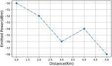
Figure 2. Emitted power of the proposed model.

Figure 3 shows the base station (BS)antenna gain of the proposed model. The BS antenna gain of the proposed model is in the ranges between −15 dBi to −10 dBi with the distance ranging from 1 km to 5 km. The proposed model has BS high antenna gain because the SGD optimization algorithm increases the overall efficiency. Moreover, when the wavelength is high, the BS antenna gain is also maximum. The number of KNNs in the proposed method for BS antenna gain significantly impacts prediction accuracy. With a smaller K value, such as K = 1, predictions are highly sensitive to noise or outliers, potentially leading to erratic estimations. An optimal K value balances bias and variance, capturing the underlying complexities of antenna gain while avoiding overfitting or under fitting, crucial for accurate BS antenna gain estimations.

Figure 3. BS antenna gain of the proposed model.

Figure 4 shows the receiver antenna gain of the proposed model. The receiver antenna gains of the proposed model range between −50 dBi and −60 dBi with the distance of the receiver ranging from 1 km to 5 km. The proposed model has a high receiver antenna gain because it uses KNN to find the nearest path. The choice of the number of nearest neighbors (K) in the KNN algorithm directly influences receiver antenna gain prediction. A smaller K value leads to increased noise sensitivity and overfitting, resulting in erratic gain estimations. Conversely, larger K values often smooth predictions, potentially averaging out important local variations and leading to a loss of fine-grained details in the gain estimation. Optimal K selection is crucial, balancing between capturing nuanced variations in gain while avoiding excessive noise or oversimplification in the predictions, ultimately impacting the accuracy and precision of receiver antenna gain estimations.

Figure 4. Receiver antenna gain of the proposed model.

Comparison results of the proposed UHF PLP based on KNNs

This section highlights the proposed UHF PLP based on KNNs and the achieved outcome was explained in detail in this section by comparing it to the outcomes of existing approaches such as AdaBoost, random forest, SVM, and BPNN [2].

Figure 5 shows the comparison of the MAE of the proposed model. The proposed model attains the minimum MAE error of 3.0 dB whereas, the existing techniques such as AdaBoost, random forest, SVM, and BPNN attain the MAE error of 6.3 dB, 6.0 dB, 4.0 dB, and 3.3 dB respectively. The MAE of the proposed model achieves a low value when compared with other existing techniques.

Figure 5. Comparison of MAE of the proposed model with existing models.

Figure 6 shows the comparison of the RMSE comparison of the proposed model. The RMSE of the proposed model achieves a low value of 3.5 dB while compared with other existing techniques such as AdaBoost, random forest, SVM, and BPNN attaining the RMSE of 6.7 dB, 6.5 dB, 5.0 dB, and 3.9 dB respectively.

Figure 6. Comparison of RMSE of the proposed model with existing models.

Figure 7 shows the comparison of the mean absolute percentage error (MAPE) comparison of the proposed model. The proposed model attains the minimum MAPE of 4% whereas, the existing techniques such as AdaBoost, random forest, SVM, and BPNN attain the MAPE of 11%, 10%, 6.3%, and 5.1% respectively. The MAPE for the proposed model attains low when compared with other existing techniques. Hence, the proposed model performs well.

Figure 7. MAPE comparison of the proposed model with the existing models.

Figure 8 shows the path loss comparison of the proposed model with the existing model. The proposed model attains the minimum path loss of 44 dB whereas, the existing techniques such as AdaBoost, random forest, SVM, and BPNN attain the MAPE path loss of 72 dB, 70 dB, 67 dB, and 50 dB respectively. When the proposed system is compared with other existing techniques the proposed model has less path loss. As a result, the proposed model is more efficient than the existing model.

Figure 8. Path loss comparison of the proposed model with the existing models.

Table 1 depicts the comparison of various parameters with various methodologies. To evaluate the effectiveness of the proposed model, existing techniques such as AdaBoost, random forest, SVM, and BPNN are compared with the proposed model. The value of MAE for AdaBoost is 6.3 dB, random forest attains 6.0 dB, SVM attains 4.0 dB, BPNN attains 3.3 dB, and proposed attains 3.0 dB. The value of RMSE attained by AdaBoost is 6.7 dB, random forest at 6.5 dB, SVM at 5.0 dB, BPNN at 3.9 dB, and the proposed method at 3.5 dB. The value of MAPE attained by AdaBoost at 11%, random forest at 10%, SVM at 6.3%, BPNN at 5.1%, and the proposed method at 4%. The value of path loss obtained by AdaBoost at 72 dB, random forest at 70 dB, SVM at 67 dB, BPNN at 50 dB, and the proposed model at 44 dB. Hence, the proposed model performs well when compared with other existing techniques.

Table 1. Overall table for the comparison of the previous model and the proposed model

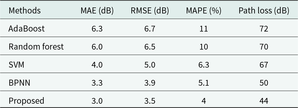
Figure 9 shows the comparison of standard deviation for proposed model with existing works. The proposed model attains minimum standard deviation of 8.07 dB. Here the proposed model is compared with existing models such as Alpha-Beta-Gamma (ABG)model, Close-In (CI) model and DL. While comparing these models with proposed method, the existing work ABG model obtains 13.84 dB, CI model obtains 13.97 dB, and the DL model obtains the standard deviation value of 9.13 dB. Hence the proposed method achieves the better standard deviation when compared to other existing models.

Figure 9. Comparison of standard deviation of the proposed model with existing works.

Figure 10 compares the Error standard deviation (ESD)of the proposed model with the existing works such as AdaBoost, SVR, BPNN and log distance. While comparing the proposed work with the existing models, the proposed method achieves 6.57 ESD. Here the existing work AdaBoost attains the ESD value of 4.15 dB, SVR attains 5.34 dB, BPNN attains the value of 5.68 dB and the log distance model achieves the ESD of 6.32 dB. Hence the proposed model achieves better value of ESD when compared with the existing models.

Figure 10. Comparison of ESD of the proposed model with existing models.

Figure 11 depicts the comparison of maxPE for proposed method with the existing works such as AdaBoost, SVR, BPNN, and log distance. When comparing the proposed model with existing works, the proposed model achieves the maxPE of 23.78 dB. The existing model AdaBoost attains the maxPE of 13.08 dB, SVR attains 13.28 dB, BPNN attains 14.83 dB, and log distance attains 21.63 dB. Here the proposed model attains the high value of maxPE.

Figure 11. Comparison of maxPE of the proposed method with existing works.

Figure 12 shows the comparison for running time of the proposed method. Here the proposed method is compared with the existing models such as SVR, Decision tree (DT), Random forest (RF) and ANN. When comparing with the existing models, proposed method attains the running time of 0.078 s, while the existing model SVR obtains 3.86 s, DT obtains 0.14 s, RF obtains 11.247 s, and ANN achieves the running time of 59.14 s. Hence the proposed model achieves low running time while the existing ANN is maximum.

Figure 12. Comparison of running time of the proposed method with existing models.

Overall, the proposed model shows that it is more efficient to predict path loss when compared to other existing techniques such as AdaBoost, random forest, SVM, and BNPP. The proposed UHF PLP based on KNNs has a low path loss of 45 dB, low MAPE of 4%, low RMSE of 3.5 dB, low MAE of 3.0 dB, standard deviation of 8.07 dB, ESD of 6.57 dB, maxPE of 23.78 dB, and running time of 0.078 s. The overall performance of the proposed model outperforms all existing models.

Conclusion

To predict and optimize the path loss in UHF wireless networks, a novel UHF PLP based on KNNs has been proposed to enhance and identify the path loss in UHF. The proposed model utilizes the KNN model to predict the path loss in the wireless network by determining the K-nearest data points to a particular test point based on a distance metric. The data is gathered from the UHF wireless network which uses the 455 MHz band and then the data is pre-processed to remove the noise in the data. The min-max scaling is used to fit the data in a specific range and distance-based feature extraction is used to extract the feature in the dataset. The KNN is used to predict the path loss by determining the KNNs for each data point. Therefore, the KNN predicts the path loss in the network. To minimize the error between the predicted values and the actual values for the optimization of the wireless network, an optimization algorithm named the SGD technique is used. To optimize the parameters of the KNN model and the results obtained by the proposed model are more accurate and efficient when compared to the various existing PLP models. The proposed model attains a low value in MAE of 3.0 dB, low RMSE of 3.5 dB, low MAPE of 4 dB, low path loss of 45 dB, standard deviation of 8.07 dB, ESD of 6.57 dB, maxPE of 23.78 dB, and running time of 0.078 s when compared to existing models such as AdaBoost, random forest, SVM, and BNPP which is 30% lower than the existing technique. Thus, the proposed model is used for the prediction and optimization of path loss in UHF wireless networks to improve the communication link and enhance the overall system performance. Overall, the UHF PLP based on KNNs is a promising approach for PLP in UHF wireless networks.