


1 Introduction
The derived category of coherent sheaves on an algebraic variety plays a crucial role in modern algebraic geometry and its related fields. In this article, we focus on exploring the categorical actions of a specific algebra—the shifted 0-affine algebra—on the derived categories of coherent sheaves on Grassmannians and n-step partial flag varieties.
1.1 Categorical
 $\mathfrak {sl}_{2}$
-Action
$\mathfrak {sl}_{2}$
-Action

Roughly speaking, a categorical action of a Kac-Moody Lie algebra
 $\mathfrak {g}$
consists of a collection of functors and categories that recover actions of Chevalley generators at the level of Grothendieck groups. Let
$\mathfrak {g}$
consists of a collection of functors and categories that recover actions of Chevalley generators at the level of Grothendieck groups. Let
 $\{e,h,f\}$
be elements in
$\{e,h,f\}$
be elements in
 $\mathfrak {g}$
that form an
$\mathfrak {g}$
that form an
 $\mathfrak {sl}_{2}$
-triple.
$\mathfrak {sl}_{2}$
-triple.
A finite-dimensional representation V of
 $\mathfrak {sl}_{2}$
consists of a direct sum decomposition
$\mathfrak {sl}_{2}$
consists of a direct sum decomposition
 $V=\oplus _{\lambda }V_{\lambda }$
into weight spaces and linear maps
$V=\oplus _{\lambda }V_{\lambda }$
into weight spaces and linear maps
 $e:V_{\lambda }\rightarrow V_{\lambda +2}$
and
$e:V_{\lambda }\rightarrow V_{\lambda +2}$
and
 $f:V_{\lambda }\rightarrow V_{\lambda -2}$
, satisfying the relation
$f:V_{\lambda }\rightarrow V_{\lambda -2}$
, satisfying the relation
 $(ef-fe)|_{V_{\lambda }}=\lambda I_{V_{\lambda }}$
. Such data can be depicted in the following diagram
$(ef-fe)|_{V_{\lambda }}=\lambda I_{V_{\lambda }}$
. Such data can be depicted in the following diagram

This characterization leads to the following notion of
 $\mathfrak {sl}_{2}$
acting on categories.
$\mathfrak {sl}_{2}$
acting on categories.
Definition 1.1 [Reference Kamnitzer28, Definition 1.2].
A naive categorical
 $\mathfrak {sl}_{2}$
-action consists of a sequence of additive categories
$\mathfrak {sl}_{2}$
-action consists of a sequence of additive categories
 $\mathcal {C}(\lambda )$
together with additive functors
$\mathcal {C}(\lambda )$
together with additive functors
 $\mathsf {E}:\mathcal {C}(\lambda ) \rightarrow \mathcal {C}(\lambda +2)$
and
$\mathsf {E}:\mathcal {C}(\lambda ) \rightarrow \mathcal {C}(\lambda +2)$
and
 $\mathsf {F}:\mathcal {C}(\lambda ) \rightarrow \mathcal {C}(\lambda -2)$
for each
$\mathsf {F}:\mathcal {C}(\lambda ) \rightarrow \mathcal {C}(\lambda -2)$
for each
 $\lambda \in \mathbb {Z}$
such that there exist isomorphisms of functorsFootnote
1
$\lambda \in \mathbb {Z}$
such that there exist isomorphisms of functorsFootnote
1
 $$ \begin{align} &\mathsf{{E}\mathsf{F}}|_{\mathcal{C}(\lambda)} \cong \mathsf{{F}\mathsf{E}}|_{\mathcal{C}(\lambda)} \bigoplus Id_{\mathcal{C}(\lambda)}^{\oplus \lambda} \ \text{if} \ \lambda \geq 0, \nonumber\\ &\mathsf{{F}\mathsf{E}}|_{\mathcal{C}(\lambda)} \cong \mathsf{{E}\mathsf{F}}|_{\mathcal{C}(\lambda)} \bigoplus Id_{\mathcal{C}(\lambda)}^{\oplus -\lambda} \ \text{if} \ \lambda \leq 0, \end{align} $$
where
 $Id_{\mathcal {C}(\lambda )}$
is the identity functor for
$Id_{\mathcal {C}(\lambda )}$
is the identity functor for
 $\mathcal {C}(\lambda )$
.
$\mathcal {C}(\lambda )$
.
The work of Beilinson-Lusztig-MacPherson [Reference Beilinson, Lusztig and MacPherson8] offers a geometric framework for a categorical
 $\mathfrak {sl}_2$
-action, where the weight categories are defined as
$\mathfrak {sl}_2$
-action, where the weight categories are defined as
 $\mathcal {C}(\lambda ) = \mathrm {D}^b\mathrm {Con}(\mathrm {Gr}(k, N))$
. These categories correspond to the derived categories of constructible sheaves on Grassmannians
$\mathcal {C}(\lambda ) = \mathrm {D}^b\mathrm {Con}(\mathrm {Gr}(k, N))$
. These categories correspond to the derived categories of constructible sheaves on Grassmannians
 $\mathrm {Gr}(k, N)$
, with
$\mathrm {Gr}(k, N)$
, with
 $\lambda = N - 2k$
. The functor
$\lambda = N - 2k$
. The functor
 $\mathsf {E}:\mathrm {D}^b\mathrm {Con}(\mathrm {Gr}(k,N)) \rightarrow \mathrm {D}^b\mathrm {Con}(\mathrm {Gr}(k-1,N))$
is given by pull-push along the following correspondence
$\mathsf {E}:\mathrm {D}^b\mathrm {Con}(\mathrm {Gr}(k,N)) \rightarrow \mathrm {D}^b\mathrm {Con}(\mathrm {Gr}(k-1,N))$
is given by pull-push along the following correspondence

where
 $\mathrm {Fl}(k-1,k)$
is the
$\mathrm {Fl}(k-1,k)$
is the
 $3$
-step partial flag variety, and the numbers above the inclusions indicate the increase in dimensions. The functor
$3$
-step partial flag variety, and the numbers above the inclusions indicate the increase in dimensions. The functor
 $\mathsf {F}$
is given by the opposite pull-push.
$\mathsf {F}$
is given by the opposite pull-push.
Then, building on the work by Beilinson-Lusztig-MacPherson [Reference Beilinson, Lusztig and MacPherson8] and Chuang-Rouquier [Reference Chuang and Rouquier20], the categories
 $\mathcal {C}(\lambda )$
and the functors
$\mathcal {C}(\lambda )$
and the functors
 $\mathsf {E}$
and
$\mathsf {E}$
and
 $\mathsf {F}$
introduced above give a naive categorical
$\mathsf {F}$
introduced above give a naive categorical
 $\mathfrak {sl}_{2}$
-action. More precisely, the functors
$\mathfrak {sl}_{2}$
-action. More precisely, the functors
 $\mathsf {E}$
and
$\mathsf {E}$
and
 $\mathsf {F}$
satisfy (1.2) in Definition 1.1.
$\mathsf {F}$
satisfy (1.2) in Definition 1.1.
The term “naive categorical action” is used in this context since the natural isomorphisms in (1.2) are not explicitly defined. In contrast, a categorical
 $\mathfrak {sl}_{2}$
-action specifies these natural isomorphisms through certain adjunctions. For a detailed explanation, please refer to [Reference Kamnitzer28, Definition 1.5].
$\mathfrak {sl}_{2}$
-action specifies these natural isomorphisms through certain adjunctions. For a detailed explanation, please refer to [Reference Kamnitzer28, Definition 1.5].
The study of natural transformations between functors is a fundamental problem in higher representation theory, particularly in the context of categorical actions. Ideally, isomorphisms between functors, such as (1.2), should arise naturally from specific adjunction data. One solution to this problem in the case of
 $\mathfrak {sl}_{2}$
-categorification was proposed by Chuang-Rouquier [Reference Chuang and Rouquier20] and later extended to (simply-laced) Kac-Moody algebras
$\mathfrak {sl}_{2}$
-categorification was proposed by Chuang-Rouquier [Reference Chuang and Rouquier20] and later extended to (simply-laced) Kac-Moody algebras
 $\mathfrak {g}$
by Khovanov-Lauda [Reference Khovanov and Lauda29] [Reference Khovanov and Lauda30] [Reference Khovanov and Lauda31], and Rouquier [Reference Rouquier38].
$\mathfrak {g}$
by Khovanov-Lauda [Reference Khovanov and Lauda29] [Reference Khovanov and Lauda30] [Reference Khovanov and Lauda31], and Rouquier [Reference Rouquier38].
Since then, there have been numerous developments and applications. In particular, people have extensively studied the categorical action of Lie algebra or quantum groups in several flavors. One of them is the notion of geometric categorical
 $\mathfrak {sl}_2$
-action, which was introduced by Cautis-Kamnitzer-Licata in [Reference Cautis, Kamnitzer and Licata16] by using Fourier-Mukai transformations. See [Reference Cautis, Kamnitzer and Licata15], [Reference Cautis, Kamnitzer and Licata17] for the applications.
$\mathfrak {sl}_2$
-action, which was introduced by Cautis-Kamnitzer-Licata in [Reference Cautis, Kamnitzer and Licata16] by using Fourier-Mukai transformations. See [Reference Cautis, Kamnitzer and Licata15], [Reference Cautis, Kamnitzer and Licata17] for the applications.
1.2 Constructing Categorical Action via Derived Categories of Coherent Sheaves
1.2.1 Main results
Our work is motivated by previous studies on constructible sheaves, and we shift our focus to categories of coherent sheaves. This leads us to consider weight categories
 $\mathcal {K}(\lambda )=\mathrm {D}^b\mathrm {Coh}(\mathrm {Gr}(k,N))$
, which are the bounded derived categories of coherent sheaves on the Grassmannian variety
$\mathcal {K}(\lambda )=\mathrm {D}^b\mathrm {Coh}(\mathrm {Gr}(k,N))$
, which are the bounded derived categories of coherent sheaves on the Grassmannian variety
 $\mathrm {Gr}(k,N)$
.
$\mathrm {Gr}(k,N)$
.
In the coherent setting,
 $\mathrm {Fl}(k-1,k)$
naturally admits a line bundle given by the quotient of the tautological bundles
$\mathrm {Fl}(k-1,k)$
naturally admits a line bundle given by the quotient of the tautological bundles
 $\mathcal {V}/\mathcal {V}'$
, where
$\mathcal {V}/\mathcal {V}'$
, where
 $\mathcal {V}$
and
$\mathcal {V}$
and
 $\mathcal {V}'$
are of rank k and
$\mathcal {V}'$
are of rank k and
 $k-1$
, respectively.
$k-1$
, respectively.
In contrast to the constructible setting, where the functors are given by a pull-push along the correspondence (1.3), in the coherent setting, we obtain a family of functors that depends on powers of the tautological line bundle
 $\mathcal {V}/\mathcal {V}'$
on
$\mathcal {V}/\mathcal {V}'$
on
 $\mathrm {Fl}(k-1,k)$
. In other words, we have a family of functors parameterized by the integers corresponding to the tensor powers of
$\mathrm {Fl}(k-1,k)$
. In other words, we have a family of functors parameterized by the integers corresponding to the tensor powers of
 $\mathcal {V}/\mathcal {V}'$
and
$\mathcal {V}/\mathcal {V}'$
and
 $(\mathcal {V}/\mathcal {V}')^{-1}$
.
$(\mathcal {V}/\mathcal {V}')^{-1}$
.
More precisely, we have for each
 $r \in \mathbb {Z}$
 $$ \begin{align} \mathsf{E}_{r}:=p_{2*}(p_{1}^{*}\otimes(\mathcal{V}/\mathcal{V}')^{\otimes r}):\mathrm{D}^b\mathrm{Coh}(\mathrm{Gr}(k,N)) \rightarrow \mathrm{D}^b\mathrm{Coh}(\mathrm{Gr}(k-1,N)) \end{align} $$
and similarly for
 $\mathsf {F}_{r}$
in the opposite direction. The main goal of this article is to study the following problem.
$\mathsf {F}_{r}$
in the opposite direction. The main goal of this article is to study the following problem.
Problem: Our goal is to investigate the algebraic structure arising from the action of the functors
 $\mathsf {E}_{r}$
and
$\mathsf {E}_{r}$
and
 $\mathsf {F}_{s}$
defined in (1.4) on the category
$\mathsf {F}_{s}$
defined in (1.4) on the category
 $\bigoplus _{k} \mathrm {D}^b\mathrm {Coh}(\mathrm {Gr}(k,N))$
. This algebra is generated by the abstract symbols
$\bigoplus _{k} \mathrm {D}^b\mathrm {Coh}(\mathrm {Gr}(k,N))$
. This algebra is generated by the abstract symbols
 $e_{r}$
and
$e_{r}$
and
 $f_{s}$
, and its structure encodes important information about the categorical action on coherent sheaves. We may ask several natural questions about this algebraic structure, such as:
$f_{s}$
, and its structure encodes important information about the categorical action on coherent sheaves. We may ask several natural questions about this algebraic structure, such as:
-
1. What are the commutator relations between
$\mathsf {E}_{r}$
and
$\mathsf {F}_{s}$
in the categorical sense? -
2. What are the relations satisfied by the generators of the algebra after we take the Grothendieck group of the categories of coherent sheaves?
-
3. Assuming that we obtain the algebra in (2), can we define a categorical action of this algebra as in Definition 1.1 for
$\mathfrak {sl}_2$
?


This article provides answers to the above questions. Before we state the main result, we would like to make some remarks.
First, the algebra that we consider in this article has a close resemblance to the loop algebra
 $L\mathfrak {sl}_{2}:=\mathfrak {sl}_{2} \otimes \mathbb {C}[t,t^{-1}]$
(although they are not identical). The generators
$L\mathfrak {sl}_{2}:=\mathfrak {sl}_{2} \otimes \mathbb {C}[t,t^{-1}]$
(although they are not identical). The generators
 $e_{r}$
,
$e_{r}$
,
 $f_{s}$
bear a resemblance to
$f_{s}$
bear a resemblance to
 $e\otimes t^r$
,
$e\otimes t^r$
,
 $f\otimes t^{s}$
respectively, where
$f\otimes t^{s}$
respectively, where
 $r,s \in \mathbb {Z}$
.
$r,s \in \mathbb {Z}$
.
Second, the idea of constructing decategorified actions goes back to Nakajima’s work [Reference Nakajima37], where twists by line bundles for the loop structure appear when moving from cohomology (or Borel-Moore homology) to K-theory.
Third, upon decategorification, we obtain an algebra with a presentation similar to the shifted quantum affine algebra defined by Finkelberg-Tsymbaliuk [Reference Finkelberg and Tsymbaliuk22]. We call the resulting algebra the shifted 0-affine algebra, denoted by
 $\mathcal {U}=\dot {\mathrm {\mathbf {U}}}_{0,N}(L\mathfrak {sl}_2)$
. The term “zero” reflects that certain relations are obtained by setting
$\mathcal {U}=\dot {\mathrm {\mathbf {U}}}_{0,N}(L\mathfrak {sl}_2)$
. The term “zero” reflects that certain relations are obtained by setting
 $q = 0$
in the relations of the shifted quantum affine algebra. In Section 7, we also explore its connection to the affine 0-Hecke algebra.
$q = 0$
in the relations of the shifted quantum affine algebra. In Section 7, we also explore its connection to the affine 0-Hecke algebra.
Finally, answering these questions enables us to construct a categorical
 $\mathcal {U}$
-action on
$\mathcal {U}$
-action on
 $\bigoplus _{k}\mathrm {D}^b\mathrm {Coh}(\mathrm {Gr}(k,N))$
. Furthermore, we extend our result to the
$\bigoplus _{k}\mathrm {D}^b\mathrm {Coh}(\mathrm {Gr}(k,N))$
. Furthermore, we extend our result to the
 $\mathfrak {sl}_{n}$
case, where the Grassmannians are replaced by the n-step partial flag varieties
$\mathfrak {sl}_{n}$
case, where the Grassmannians are replaced by the n-step partial flag varieties
 $\mathrm {Fl}_{\underline {k}}(\mathbb {C}^N)$
(see (1.12) for its definition). We summarize the main results of this article in the following theorem.
$\mathrm {Fl}_{\underline {k}}(\mathbb {C}^N)$
(see (1.12) for its definition). We summarize the main results of this article in the following theorem.
Theorem 1.2.
-
1. For the values of r and s restrict to certain ranges, either
$\mathsf {E}_{i,r}\mathsf {F}_{i,s}$
and
$\mathsf {F}_{i,s}\mathsf {E}_{i,r}$
are isomorphic or there are non-split exact triangles relating them (Proposition 5.10). -
2. The resulting algebra is a new algebra, the shifted 0-affine algebra
$\mathcal {U}$
with generators and relations are given in Definition 2.6. -
3. We give a definition of categorical
$\mathcal {U}$
-action (Definition 3.1). We prove that there is a categorical
$\mathcal {U}$
-action on
$\bigoplus _{\underline {k}}\mathrm {D}^b\mathrm {Coh}(\mathrm {Fl}_{\underline {k}}(\mathbb {C}^N))$
(Theorem 5.6).


1.2.2 The difference from the constructible setting and other new features
In this subsection, we provide further details on our results, focusing specifically on the categorical commutator relations arising from the geometric setting as described in Theorem 1.2 (1).
We begin by explaining the restriction of the loop generators. This restriction stems primarily from the chosen presentation of the shifted 0-affine algebra
 $\mathcal {U}$
, defined in Definition 2.6. Inspired by the Levendorskii presentation of the shifted quantum affine algebra introduced by Finkelberg and Tsymbaliuk [Reference Finkelberg and Tsymbaliuk22] (see Definition 2.3), this presentation is particularly advantageous due to its simplicity. It employs a finite set of generators and relations for
$\mathcal {U}$
, defined in Definition 2.6. Inspired by the Levendorskii presentation of the shifted quantum affine algebra introduced by Finkelberg and Tsymbaliuk [Reference Finkelberg and Tsymbaliuk22] (see Definition 2.3), this presentation is particularly advantageous due to its simplicity. It employs a finite set of generators and relations for
 $\mathcal {U}$
, enabling a straightforward definition of a categorical
$\mathcal {U}$
, enabling a straightforward definition of a categorical
 $\mathcal {U}$
-action. More precisely, our algebra
$\mathcal {U}$
-action. More precisely, our algebra
 $\mathcal {U}$
is defined by the idempotent modification, and we only have the loop generators
$\mathcal {U}$
is defined by the idempotent modification, and we only have the loop generators
 $e_{r}1_{(k,N-k)}$
and
$e_{r}1_{(k,N-k)}$
and
 $f_s1_{(k,N-k)}$
for
$f_s1_{(k,N-k)}$
for
 ${-k} \leq r \leq 0$
and
${-k} \leq r \leq 0$
and
 $0 \leq s \leq {N-k}$
.
$0 \leq s \leq {N-k}$
.
In [Reference Finkelberg and Tsymbaliuk22], Finkelberg-Tsymbaliuk proved the equivalence between the Levendorskii presentation and the usual loop presentation of the shifted quantum affine algebra (see Theorem 2.4). In Appendix A, we introduce a definition for the shifted 0-affine algebra using the loop presentation (see Definition A.1) and conjecture that the two presentations are equivalent (see Conjecture A.4).
To compare the compositions of functors
 $\mathsf {E}_{r}\mathsf {F}_{s}$
and
$\mathsf {E}_{r}\mathsf {F}_{s}$
and
 $\mathsf {F}_{s}\mathsf {E}_{r}$
with
$\mathsf {F}_{s}\mathsf {E}_{r}$
with
 $\mathsf {E}_{r}$
,
$\mathsf {E}_{r}$
,
 $\mathsf {F}_{s}$
defined in (1.4), we use the language of Fourier-Mukai (FM) transformations. It translates the comparison between functor compositions to the comparison between convolutions of FM kernels. We denote
$\mathsf {F}_{s}$
defined in (1.4), we use the language of Fourier-Mukai (FM) transformations. It translates the comparison between functor compositions to the comparison between convolutions of FM kernels. We denote
 $\mathcal {E}_{r}\boldsymbol {1}_{(k,N-k)}$
to be the FM kernel for
$\mathcal {E}_{r}\boldsymbol {1}_{(k,N-k)}$
to be the FM kernel for
 $\mathsf {E}_{r}\boldsymbol {1}_{(k,N-k)}$
and similarly
$\mathsf {E}_{r}\boldsymbol {1}_{(k,N-k)}$
and similarly
 $\mathcal {F}_{s}\boldsymbol {1}_{(k,N-k)}$
for
$\mathcal {F}_{s}\boldsymbol {1}_{(k,N-k)}$
for
 $\mathsf {F}_{s}\boldsymbol {1}_{(k,N-k)}$
where
$\mathsf {F}_{s}\boldsymbol {1}_{(k,N-k)}$
where
 $r,s \in \mathbb {Z}$
.
$r,s \in \mathbb {Z}$
.
Due to our presentation of
 $\mathcal {U}$
, we only have to compare
$\mathcal {U}$
, we only have to compare
 $(\mathcal {E}_{r} \ast \mathcal {F}_{s})\boldsymbol {1}_{(k,N-k)}$
and
$(\mathcal {E}_{r} \ast \mathcal {F}_{s})\boldsymbol {1}_{(k,N-k)}$
and
 $(\mathcal {F}_{s}\ast \mathcal {E}_{r})\boldsymbol {1}_{(k,N-k)}$
for
$(\mathcal {F}_{s}\ast \mathcal {E}_{r})\boldsymbol {1}_{(k,N-k)}$
for
 $-k \leq r+s \leq N-k$
, where we denote
$-k \leq r+s \leq N-k$
, where we denote
 $\ast $
to be the convolution of FM kernels.
$\ast $
to be the convolution of FM kernels.
When
 $-k+1 \leq r+s \leq N-k-1$
, we then obtain the following isomorphisms
$-k+1 \leq r+s \leq N-k-1$
, we then obtain the following isomorphisms
 $$ \begin{align} (\mathcal{E}_{r} \ast \mathcal{F}_{s})\boldsymbol{1}_{(k,N-k)} \cong (\mathcal{F}_{s}\ast \mathcal{E}_{r})\boldsymbol{1}_{(k,N-k)}. \end{align} $$
When
 $r+s=N-k$
and
$r+s=N-k$
and
 $r+s=-k$
, we only have the two cases
$r+s=-k$
, we only have the two cases
 $(r,s)=(0,N-k)$
and
$(r,s)=(0,N-k)$
and
 $(r,s)=(-k,0)$
respectively. Then, we have the following exact triangles in
$(r,s)=(-k,0)$
respectively. Then, we have the following exact triangles in
 $\mathrm {D}^b\mathrm {Coh}(\mathrm {Gr}(k,N) \times \mathrm {Gr}(k,N))$
 $$ \begin{align} &({\mathcal{F}}_{{N-k}} \ast {\mathcal{E}}_{{0}})\boldsymbol{1}_{(k,N-k)} \rightarrow ({\mathcal{E}}_{{0}}\ast {\mathcal{F}}_{{N-k}})\boldsymbol{1}_{(k,N-k)} \rightarrow {\Psi}^{+}\boldsymbol{1}_{(k,N-k)}, \end{align} $$
 $$ \begin{align} &({\mathcal{E}}_{{-k}} \ast {\mathcal{F}}_{{0}})\boldsymbol{1}_{(k,N-k)} \rightarrow ({\mathcal{F}}_{{0}}\ast {\mathcal{E}}_{{-k}})\boldsymbol{1}_{(k,N-k)} \rightarrow {\Psi}^{-}\boldsymbol{1}_{(k,N-k)}, \end{align} $$
where
 ${\Psi }^{+}\boldsymbol {1}_{(k,N-k)}$
,
${\Psi }^{+}\boldsymbol {1}_{(k,N-k)}$
,
 ${\Psi }^{-}\boldsymbol {1}_{(k,N-k)}$
are certain FM kernels (see Definition 5.5 for details).
${\Psi }^{-}\boldsymbol {1}_{(k,N-k)}$
are certain FM kernels (see Definition 5.5 for details).
Remark 1.3. By using the conjugation property for
 $\mathsf {E}_{r}\boldsymbol {1}_{(k,N-k)}$
and
$\mathsf {E}_{r}\boldsymbol {1}_{(k,N-k)}$
and
 $\mathsf {F}_{s}\boldsymbol {1}_{(k,N-k)}$
(see condition (7)(a) and (8)(a) in Definition 3.1), we obtain that the above exact triangles (1.6) and (1.7) also hold for
$\mathsf {F}_{s}\boldsymbol {1}_{(k,N-k)}$
(see condition (7)(a) and (8)(a) in Definition 3.1), we obtain that the above exact triangles (1.6) and (1.7) also hold for
 $(\mathcal {E}_{r} \ast \mathcal {F}_{s})\boldsymbol {1}_{(k,N-k)}$
and
$(\mathcal {E}_{r} \ast \mathcal {F}_{s})\boldsymbol {1}_{(k,N-k)}$
and
 $(\mathcal {F}_{s}\ast \mathcal {E}_{r})\boldsymbol {1}_{(k,N-k)}$
when
$(\mathcal {F}_{s}\ast \mathcal {E}_{r})\boldsymbol {1}_{(k,N-k)}$
when
 $r+s=N-k$
and
$r+s=N-k$
and
 $r+s=-k$
respectively (see (3.5)).
$r+s=-k$
respectively (see (3.5)).
We highlight some key properties of the above results. Firstly, it’s worth noting that the commutator between
 $\mathsf {E}_{r}$
and
$\mathsf {E}_{r}$
and
 $\mathsf {F}_{s}$
depends only on the integer
$\mathsf {F}_{s}$
depends only on the integer
 $r+s$
provided
$r+s$
provided
 $-k \leq r+s \leq N-k$
. Secondly, the isomorphisms (1.5) and exact triangles (1.6), (1.7) are closely related to the coherent sheaf cohomology
$-k \leq r+s \leq N-k$
. Secondly, the isomorphisms (1.5) and exact triangles (1.6), (1.7) are closely related to the coherent sheaf cohomology
 $H^{*}(\mathbb {P}^{N-1}, \mathcal {O}_{\mathbb {P}^{N-1}}(-r-s-k))$
. Specifically, (1.5) corresponds to the vanishing
$H^{*}(\mathbb {P}^{N-1}, \mathcal {O}_{\mathbb {P}^{N-1}}(-r-s-k))$
. Specifically, (1.5) corresponds to the vanishing
 $H^{*}(\mathbb {P}^{N-1}, \mathcal {O}_{\mathbb {P}^{N-1}}(-r-s-k))=0$
for
$H^{*}(\mathbb {P}^{N-1}, \mathcal {O}_{\mathbb {P}^{N-1}}(-r-s-k))=0$
for
 $-N+1 \leq -r-s-k \leq -1$
, which in turn implies
$-N+1 \leq -r-s-k \leq -1$
, which in turn implies
 $[e_{r},f_{s}]1_{(k,N-k)}=0$
when
$[e_{r},f_{s}]1_{(k,N-k)}=0$
when
 $1-k \leq r+s \leq N-k-1$
. Thirdly, the exact triangles (1.6), (1.7) are non-split, as we discuss in Remark 5.11, which is different from the corresponding constructible setting ((1.2) in Definition 1.1).
$1-k \leq r+s \leq N-k-1$
. Thirdly, the exact triangles (1.6), (1.7) are non-split, as we discuss in Remark 5.11, which is different from the corresponding constructible setting ((1.2) in Definition 1.1).
1.2.3 Toward a future study
Although our presentation of
 $\mathcal {U}$
does not cover all the loop generators, the FM kernels
$\mathcal {U}$
does not cover all the loop generators, the FM kernels
 $\mathcal {E}_r \boldsymbol {1}_{(k, N-k)}$
and
$\mathcal {E}_r \boldsymbol {1}_{(k, N-k)}$
and
 $\mathcal {F}_s \boldsymbol {1}_{(k, N-k)}$
are defined for all
$\mathcal {F}_s \boldsymbol {1}_{(k, N-k)}$
are defined for all
 $r, s \in \mathbb {Z}$
. Therefore, it is of interest to explore the relations between
$r, s \in \mathbb {Z}$
. Therefore, it is of interest to explore the relations between
 $(\mathcal {E}_r \ast \mathcal {F}_s)\boldsymbol {1}_{(k, N-k)}$
and
$(\mathcal {E}_r \ast \mathcal {F}_s)\boldsymbol {1}_{(k, N-k)}$
and
 $(\mathcal {F}_s \ast \mathcal {E}_r)\boldsymbol {1}_{(k, N-k)}$
for
$(\mathcal {F}_s \ast \mathcal {E}_r)\boldsymbol {1}_{(k, N-k)}$
for
 $r + s \geq N - k + 1$
and
$r + s \geq N - k + 1$
and
 $r + s \leq -k - 1$
. In this article, we provide an initial exploration of the case where
$r + s \leq -k - 1$
. In this article, we provide an initial exploration of the case where
 $r + s = N - k + 1$
(and similarly
$r + s = N - k + 1$
(and similarly
 $r + s = -k - 1$
), as discussed in Section 6.
$r + s = -k - 1$
), as discussed in Section 6.
Like (1.6) and (1.7), we obtain the following (non-split) exact triangles in
 $\mathrm {D}^b\mathrm {Coh}(\mathrm {Gr}(k,N) \times \mathrm {Gr}(k,N))$
 $$ \begin{align} &({\mathcal{F}}_{N-k+1} \ast {\mathcal{E}}_{0})\mathbf{1}_{(k,N-k)} \rightarrow ({\mathcal{E}}_{0}\ast {\mathcal{F}}_{N-k+1})\mathbf{1}_{(k,N-k)} \rightarrow ({\Psi}^{+} \ast \mathcal{H}_{1})\mathbf{1}_{(k,N-k)}, \end{align} $$
 $$ \begin{align} &({\mathcal{E}}_{-k-1} \ast {\mathcal{F}}_{0})\mathbf{1}_{(k,N-k)} \rightarrow ({\mathcal{F}}_{0}\ast {\mathcal{E}}_{-k-1})\mathbf{1}_{(k,N-k)} \rightarrow ({\Psi}^{-} \ast \mathcal{H}_{-1})\mathbf{1}_{(k,N-k)}, \end{align} $$
where
 $\mathcal {H}_{\pm 1}\boldsymbol {1}_{(k,N-k)}$
are certain FM kernels (see (6.7) and (6.8)).
$\mathcal {H}_{\pm 1}\boldsymbol {1}_{(k,N-k)}$
are certain FM kernels (see (6.7) and (6.8)).
The exact triangles (1.8) and (1.9) can be viewed as categorifications of the two commutators
 $[e_0,f_{N-k+1}]1_{(k,N-k)}$
and
$[e_0,f_{N-k+1}]1_{(k,N-k)}$
and
 $[e_{-k-1},f_{0}]1_{(k,N-k)}$
respectively. Although the elements
$[e_{-k-1},f_{0}]1_{(k,N-k)}$
respectively. Although the elements
 $e_{-k-1}1_{(k,N-k)}$
and
$e_{-k-1}1_{(k,N-k)}$
and
 $f_{N-k+1}1_{(k,N-k)}$
are not included in the generators of
$f_{N-k+1}1_{(k,N-k)}$
are not included in the generators of
 $\mathcal {U}$
, the conjugation property of the FM kernels
$\mathcal {U}$
, the conjugation property of the FM kernels
 $\mathcal {E}_{r} \boldsymbol {1}_{(k,N-k)}$
and
$\mathcal {E}_{r} \boldsymbol {1}_{(k,N-k)}$
and
 $\mathcal {F}_{s} \boldsymbol {1}_{(k,N-k)}$
(see (6.4)) suggests that we can define
$\mathcal {F}_{s} \boldsymbol {1}_{(k,N-k)}$
(see (6.4)) suggests that we can define
 $e_{-k-1} 1_{(k,N-k)}$
and
$e_{-k-1} 1_{(k,N-k)}$
and
 $f_{N-k+1} 1_{(k,N-k)}$
in
$f_{N-k+1} 1_{(k,N-k)}$
in
 $\mathcal {U}$
by using conjugation with
$\mathcal {U}$
by using conjugation with
 $\psi ^+ 1_{(k,N-k)}$
(see (6.5)). Finally, we define
$\psi ^+ 1_{(k,N-k)}$
(see (6.5)). Finally, we define
which are elements of
 $\mathcal {U}$
, ensuring that (1.8) and (1.9) categorify the desired commutator relations.
$\mathcal {U}$
, ensuring that (1.8) and (1.9) categorify the desired commutator relations.
Let
 $\mathsf {{H}}_{\pm 1}\boldsymbol {1}_{(k,N-k)}$
denote the FM transformations with kernels given by
$\mathsf {{H}}_{\pm 1}\boldsymbol {1}_{(k,N-k)}$
denote the FM transformations with kernels given by
 $\mathcal {H}_{\pm 1} \boldsymbol {1}_{(k,N-k)}$
. These transformations categorify
$\mathcal {H}_{\pm 1} \boldsymbol {1}_{(k,N-k)}$
. These transformations categorify
 $h_{\pm 1} 1_{(k,N-k)}$
, which can be viewed as an analog of the loop-Cartan-type elements in the quantum loop algebra
$h_{\pm 1} 1_{(k,N-k)}$
, which can be viewed as an analog of the loop-Cartan-type elements in the quantum loop algebra
 $\boldsymbol {\mathrm {U}}_{q}(L\mathfrak {sl}_2)$
. For the sake of completeness, it would be appropriate to include the 1-morphisms
$\boldsymbol {\mathrm {U}}_{q}(L\mathfrak {sl}_2)$
. For the sake of completeness, it would be appropriate to include the 1-morphisms
 $\mathsf {{H}}_{\pm 1} \boldsymbol {1}_{(k,N-k)}$
and certain exact triangles, such as (1.8) and (1.9), as conditions in a categorical
$\mathsf {{H}}_{\pm 1} \boldsymbol {1}_{(k,N-k)}$
and certain exact triangles, such as (1.8) and (1.9), as conditions in a categorical
 $\mathcal {U}$
-action. However, this article does not include these conditions, as we have not yet identified any direct applications for the 1-morphisms
$\mathcal {U}$
-action. However, this article does not include these conditions, as we have not yet identified any direct applications for the 1-morphisms
 $\mathsf {{H}}_{\pm 1} \boldsymbol {1}_{(k,N-k)}$
.
$\mathsf {{H}}_{\pm 1} \boldsymbol {1}_{(k,N-k)}$
.
Although we do not include
 $\mathsf {{H}}_{\pm 1} \boldsymbol {1}_{(k,N-k)}$
and the conditions involving them in our definition of a categorical
$\mathsf {{H}}_{\pm 1} \boldsymbol {1}_{(k,N-k)}$
and the conditions involving them in our definition of a categorical
 $\mathcal {U}$
-action, we believe that studying the properties of
$\mathcal {U}$
-action, we believe that studying the properties of
 $\mathsf {{H}}_{\pm 1} \boldsymbol {1}_{(k,N-k)}$
and their associated FM kernels
$\mathsf {{H}}_{\pm 1} \boldsymbol {1}_{(k,N-k)}$
and their associated FM kernels
 $\mathcal {H}_{\pm 1} \boldsymbol {1}_{(k,N-k)}$
remains valuable, which is in Section 6. Moreover, such exploration can provide deeper insights into the structure and behavior of the categorical
$\mathcal {H}_{\pm 1} \boldsymbol {1}_{(k,N-k)}$
remains valuable, which is in Section 6. Moreover, such exploration can provide deeper insights into the structure and behavior of the categorical
 $\mathcal {U}$
-action.
$\mathcal {U}$
-action.
We summarize the results in the following proposition.
Proposition 1.4.
-
1. Assuming that certain exact triangles like (1.8) and (1.9) exist as a condition in a categorical
$\mathcal {U}$
-action, then
$\mathsf {{H}}_{\pm 1}\boldsymbol {1}_{(k,N-k)}$
are biadjoint to each other up to conjugation by
$\mathsf {\Psi }^{\pm }\boldsymbol {1}_{(k,N-k)}$
(Lemma 6.1). -
2. For the FM kernel
$\mathcal {H}_{1}\boldsymbol {1}_{(k,N-k)}$
, there exists the following exact triangle: where
$$ \begin{align*} \Delta_{*}\mathcal{V} \rightarrow \mathcal{H}_1\boldsymbol{1}_{(k,N-k)} \rightarrow \Delta_*\mathbb{C}^N/\mathcal{V} \in \mathrm{D}^b\mathrm{Coh}(\mathrm{Gr}(k,N) \times \mathrm{Gr}(k,N)) \end{align*} $$
$\Delta :\mathrm {Gr}(k,N) \rightarrow \mathrm {Gr}(k,N) \times \mathrm {Gr}(k,N)$
is the diagonal map. Moreover,
$\mathcal {H}_1\boldsymbol {1}_{(k,N-k)}$
is neither isomorphic to
$\Delta _*\mathbb {C}^N$
nor to
$\Delta _*(\mathcal {V} \oplus \mathbb {C}^N/\mathcal {V})$
, provided
$k \neq 0,N$
(Proposition 6.2).
-
3. We compute the convolutions between
$\mathcal {H}_1\boldsymbol {1}_{(k,N-k)}$
and
$\Psi ^+\boldsymbol {1}_{(k,N-k)}$
,
$\mathcal {E}_r\boldsymbol {1}_{(k,N-k)}$
in the simplest case where
$k=1$
and
$N=2$
.-
(a) We have the non-isomorphism
$(\mathcal {H}_1 \ast \Psi ^+)\boldsymbol {1}_{(1,1)} \ncong (\Psi ^+ \ast \mathcal {H}_1)\boldsymbol {1}_{(1,1)}$
, while
$h_1\psi ^+1_{(1,1)}=\psi ^+h_11_{(1,1)}$
(Proposition 6.4). -
(b) There exists the exact triangle (Proposition 6.6)
$$ \begin{align*} (\mathcal{H}_1 \ast \mathcal{E}_{-1})\boldsymbol{1}_{(1,1)} \rightarrow (\mathcal{E}_{-1} \ast \mathcal{H}_1)\boldsymbol{1}_{(1,1)} \rightarrow \mathcal{E}_0\boldsymbol{1}_{(1,1)} \oplus \mathcal{E}_0\boldsymbol{1}_{(1,1)}[1] \in \mathrm{D}^b\mathrm{Coh}(\mathbb{P}^1), \end{align*} $$
$[h_1,e_{-1}]1_{(1,1)}=0$
. Finally, we propose a conjecture (Conjecture 6.8) about the convolution relations between
${\mathcal {H}}_{\pm 1}\boldsymbol {1}_{(k,N-k)}$
and
${\mathcal {E}}_r\boldsymbol {1}_{(k,N-k)}$
,
${\mathcal {F}}_s\boldsymbol {1}_{(k,N-k)}$
.
-


1.2.4 The Grothendieck groups
Like the categorical
 $\mathfrak {sl}_2$
-action, as we expect, a categorical
$\mathfrak {sl}_2$
-action, as we expect, a categorical
 $\mathcal {U}$
-action should also recover the action of
$\mathcal {U}$
-action should also recover the action of
 $\mathcal {U}$
on the level of Grothendieck groups. We prove this in Lemma 3.5. Thus, by (3) in Theorem 1.2 (or Theorem 5.6), we obtain the following corollary.
$\mathcal {U}$
on the level of Grothendieck groups. We prove this in Lemma 3.5. Thus, by (3) in Theorem 1.2 (or Theorem 5.6), we obtain the following corollary.
Corollary 1.5 (Corollary 5.14 for
$\mathfrak {sl}_n$
case).

There is an action of
 $\mathcal {U}$
on
$\mathcal {U}$
on
 $\bigoplus _{k} K(\mathrm {Gr}(k,N))$
.
$\bigoplus _{k} K(\mathrm {Gr}(k,N))$
.
Although we do not include all the loop generators in our presentation of
 $\mathcal {U}$
, with the help from the study of categorical
$\mathcal {U}$
, with the help from the study of categorical
 $\mathcal {U}$
-action on
$\mathcal {U}$
-action on
 $\bigoplus _k \mathrm {D}^b\mathrm {Coh}(\mathrm {Gr}(k,N))$
, we extend the commutator relation
$\bigoplus _k \mathrm {D}^b\mathrm {Coh}(\mathrm {Gr}(k,N))$
, we extend the commutator relation
 $[e_{r},f_{s}]1_{(k,N-k)}$
on
$[e_{r},f_{s}]1_{(k,N-k)}$
on
 $K(\mathrm {Gr}(k,N))$
in Corollary 1.5 to all
$K(\mathrm {Gr}(k,N))$
in Corollary 1.5 to all
 $r,s \in \mathbb {Z}$
. Note that here the actions of
$r,s \in \mathbb {Z}$
. Note that here the actions of
 $e_{r}1_{(k,N-k)}$
are given by the decategorified (or K-theoretic) FM transformations with kernels given by the classes of the line bundles
$e_{r}1_{(k,N-k)}$
are given by the decategorified (or K-theoretic) FM transformations with kernels given by the classes of the line bundles
 $(\mathcal {V}/\mathcal {V}')^{\otimes r}$
in the Grothendieck group
$(\mathcal {V}/\mathcal {V}')^{\otimes r}$
in the Grothendieck group
 $K(\mathrm {Fl}(k-1,k))$
, similarly for
$K(\mathrm {Fl}(k-1,k))$
, similarly for
 $f_{s}1_{(k,N-k)}$
.
$f_{s}1_{(k,N-k)}$
.
Corollary 1.6 (Corollary 6.10 for
$\mathfrak {sl}_{n}$
case).

The commutator relations in the Grothendieck group
 $K(\mathrm {Gr}(k,N))$
for
$K(\mathrm {Gr}(k,N))$
for
 $e_{r}1_{(k,N-k)}$
,
$e_{r}1_{(k,N-k)}$
,
 $f_{s}1_{(k,N-k)}$
with
$f_{s}1_{(k,N-k)}$
with
 $r,s \in \mathbb {Z}$
are given by
$r,s \in \mathbb {Z}$
are given by
 $$ \begin{align*} [e_{r},f_{s}]1_{(k,N-k)}= \begin{cases} \otimes (-1)^{N-k-1}[\det(\mathbb{C}^N/\mathcal{V})][\mathrm{Sym}^{r+s-N+k}(\mathbb{C}^N)] & \text{if} \ r+s \geq N-k \\ 0 & \text{if} \ -k+1 \leq r+s \leq N-k-1 \\ \otimes (-1)^{k}[\det(\mathcal{V})^{-1}][\mathrm{Sym}^{-r-s-k}(\mathbb{C}^N)^{\vee}]& \text{if} \ r+s \leq -k \end{cases}. \end{align*} $$
1.3 Application to the Affine 0-Hecke Algebra
In the second part of this article, we apply the categorical
 $\mathcal {U}$
-action to construct a categorical action of the affine 0-Hecke algebra, denoted by
$\mathcal {U}$
-action to construct a categorical action of the affine 0-Hecke algebra, denoted by
 $\mathcal {H}_{N}(0)$
, on the derived category of coherent sheaves on the full flag variety.
$\mathcal {H}_{N}(0)$
, on the derived category of coherent sheaves on the full flag variety.
The affine
 $0$
-Hecke algebra
$0$
-Hecke algebra
 $\mathcal {H}_{N}(0)$
arises as a specific degeneration of the affine Hecke algebra, obtained by setting
$\mathcal {H}_{N}(0)$
arises as a specific degeneration of the affine Hecke algebra, obtained by setting
 $q=0$
in its relations. It was first introduced in the work of Kostant and Kumar [Reference Kostant and Kumar32], where they provided a geometric realization of the affine
$q=0$
in its relations. It was first introduced in the work of Kostant and Kumar [Reference Kostant and Kumar32], where they provided a geometric realization of the affine
 $0$
-Hecke algebra via the G-equivariant K-theory of the product of full flag varieties, equipped with the convolution product.
$0$
-Hecke algebra via the G-equivariant K-theory of the product of full flag varieties, equipped with the convolution product.
The affine
 $0$
-Hecke algebra also plays a fundamental role in the study of mod p representations of p-adic reductive groups, where it appears under various names. For instance, He and Nie [Reference He and Nie24] use the term “affine pro-p Hecke algebra” in their investigation of its cocenter, while Abe [Reference Abe1] and Vignéras [Reference Vingeras39] refer to it as the “pro-p-Iwahori Hecke algebra” in their classification of irreducible representations.
$0$
-Hecke algebra also plays a fundamental role in the study of mod p representations of p-adic reductive groups, where it appears under various names. For instance, He and Nie [Reference He and Nie24] use the term “affine pro-p Hecke algebra” in their investigation of its cocenter, while Abe [Reference Abe1] and Vignéras [Reference Vingeras39] refer to it as the “pro-p-Iwahori Hecke algebra” in their classification of irreducible representations.
Analogous to the categorification of affine Hecke algebras, such as Bezrukavnikov’s two geometric realizations [Reference Bezrukavnikov11], it is natural to consider the categorification of affine
 $0$
-Hecke algebras. For example, see [Reference Arkhipov and Kanstrup4] for related developments. Building on the work of Kostant and Kumar, there is a natural action of the affine
$0$
-Hecke algebras. For example, see [Reference Arkhipov and Kanstrup4] for related developments. Building on the work of Kostant and Kumar, there is a natural action of the affine
 $0$
-Hecke algebra on the G-equivariant K-theory of the full flag variety, realized through the convolution product.
$0$
-Hecke algebra on the G-equivariant K-theory of the full flag variety, realized through the convolution product.
By forgetting the G-equivariance, our second main result of this article is to categorify the above action by lifting the action from K-theory to the derived category of coherent sheaves.
Let us elaborate on this in more detail. We fix
 $G=\mathrm {SL}_{N}(\mathbb {C})$
and let
$G=\mathrm {SL}_{N}(\mathbb {C})$
and let
 $B \subset G$
denote the Borel subgroup of upper triangular matrices. The full flag variety is described as follows:
$B \subset G$
denote the Borel subgroup of upper triangular matrices. The full flag variety is described as follows:
 $$ \begin{align} G/B=\{0=V_{0} \subset V_{1} \subset ... \subset V_{N}=\mathbb{C}^N \ | \ \dim V_{k}=k \ \text{for} \ \text{all} \ k \}, \end{align} $$
Similarly, the partial flag variety is given by
 $$ \begin{align} G/P_{i}=\{0 \subset V_{1} \subset V_{2} \subset ...V_{i-1} \subset V_{i+1} \subset ... V_{N}=\mathbb{C}^N \ | \ \dim V_{k} =k \ \text{for} \ k \neq i \} \end{align} $$
where
 $P_{i}$
is a minimal parabolic subgroup for
$P_{i}$
is a minimal parabolic subgroup for
 $1 \leq i \leq N-1$
.
$1 \leq i \leq N-1$
.
The Demazure operators, introduced by Demazure [Reference Demazure21] and rooted in the fundamental works of Bernstein-Gelfand-Gelfand [Reference Bernstein, Gelfand and Gelfand10], are defined as
Here,
 $\pi _{i}:G/B \rightarrow G/P_{i}$
denotes the natural projection, and
$\pi _{i}:G/B \rightarrow G/P_{i}$
denotes the natural projection, and
 $\pi _i^*$
and
$\pi _i^*$
and
 $\pi _{i*}$
represent the induced pullback and pushforward on the Grothendieck group, respectively, for all
$\pi _{i*}$
represent the induced pullback and pushforward on the Grothendieck group, respectively, for all
 $1 \leq i \leq N-1$
.
$1 \leq i \leq N-1$
.
On the other hand, let
 $\mathcal {V}_{i}$
denote the tautological bundle of rank i on
$\mathcal {V}_{i}$
denote the tautological bundle of rank i on
 $G/B$
for
$G/B$
for
 $0 \leq i \leq N$
. Then, for
$0 \leq i \leq N$
. Then, for
 $1 \leq i \leq N$
, we have the natural line bundles
$1 \leq i \leq N$
, we have the natural line bundles
 $\mathscr {L}_{i}=\mathcal {V}_{i}/\mathcal {V}_{i-1}$
on
$\mathscr {L}_{i}=\mathcal {V}_{i}/\mathcal {V}_{i-1}$
on
 $G/B$
.
$G/B$
.
The Demazure operators
 $T_{i}$
, together with the operators given by multiplication by the classes of the line bundles
$T_{i}$
, together with the operators given by multiplication by the classes of the line bundles
 $[\mathscr {L}_{j}]$
, generate the affine 0-Hecke algebra
$[\mathscr {L}_{j}]$
, generate the affine 0-Hecke algebra
 $\mathcal {H}_{N}(0)$
. Consequently, these operators define an action of
$\mathcal {H}_{N}(0)$
. Consequently, these operators define an action of
 $\mathcal {H}_{N}(0)$
on
$\mathcal {H}_{N}(0)$
on
 $K(G/B)$
. For the definition of
$K(G/B)$
. For the definition of
 $\mathcal {H}_{N}(0)$
, we refer the readers to Definition 7.1.
$\mathcal {H}_{N}(0)$
, we refer the readers to Definition 7.1.
The following is our second main result.
Theorem 1.7 (Theorem 7.3).
There is a categorical action of
 $\mathcal {H}_{N}(0)$
on
$\mathcal {H}_{N}(0)$
on
 $\mathrm {D}^b\mathrm {Coh}(G/B)$
.
$\mathrm {D}^b\mathrm {Coh}(G/B)$
.
One approach to proving this theorem is to directly lift the action by replacing the generators with FM transformations. However, verifying the relations for this action requires performing six convolutions of kernels and checking various exact triangles that relate them (see Theorem 7.3 for details). Instead of pursuing this direct but intricate method, we reinterpret the Demazure operators as elements of the shifted
 $0$
-affine algebra and leverage its categorical action to present a more concise and elegant proof.
$0$
-affine algebra and leverage its categorical action to present a more concise and elegant proof.
We need to introduce more notations. For each
 $\underline {k}=(k_{1},...,k_{n}) \vDash N$
, the n-step partial flag variety is defined by
$\underline {k}=(k_{1},...,k_{n}) \vDash N$
, the n-step partial flag variety is defined by
 $$ \begin{align} \mathrm{Fl}_{\underline{k}}(\mathbb{C}^N):=\{V_{\bullet}=(0=V_{0} \subset V_1 \subset ... \subset V_{n}=\mathbb{C}^N) \ | \ \mathrm{dim} V_{i}/V_{i-1}=k_{i} \ \text{for} \ \text{all} \ i\}. \end{align} $$
With this notation, the full flag variety
 $G/B$
and partial flag varieties
$G/B$
and partial flag varieties
 $G/P_{i}$
in (1.10) and (1.11) have the following description
$G/P_{i}$
in (1.10) and (1.11) have the following description
 $$ \begin{align*} G/B=\mathrm{Fl}_{(1,1,...,1)}(\mathbb{C}^N), \ G/P_{i}=\mathrm{Fl}_{(1,1,...,1)+\alpha_{i}}(\mathbb{C}^N)= \mathrm{Fl}_{(1,1,...,1)-\alpha_{i}}(\mathbb{C}^N) \end{align*} $$
where
 $\alpha _{i}=(0,...,-1,1,...,0)$
is the simple root with
$\alpha _{i}=(0,...,-1,1,...,0)$
is the simple root with
 $-1$
in the ith position and we have the following diagram
$-1$
in the ith position and we have the following diagram

By utilizing (1.13), it is possible to express the Demazure operators
 $T_{i}$
as elements within
$T_{i}$
as elements within
 $\mathcal {U}$
. This implies that all the categorical relations we need to verify can be derived from conditions in the categorical
$\mathcal {U}$
. This implies that all the categorical relations we need to verify can be derived from conditions in the categorical
 $\mathcal {U}$
-action, leading to a significant reduction in calculations.
$\mathcal {U}$
-action, leading to a significant reduction in calculations.
We would like to mention the related works of Arkhipov and Kanstrup. In their series of papers [Reference Arkhipov and Kanstrup2], [Reference Arkhipov and Kanstrup3], [Reference Arkhipov and Kanstrup4], and [Reference Arkhipov and Kanstrup5], they introduced the concept of Demazure descent data on a triangulated category as an initial attempt to comprehend the higher categorical Beilinson-Bernstein localization, which was developed by Ben-Zvi and Nalder [Reference Ben-Zvi and Nadler9]. The categorified Demazure operators from our Theorem 1.7 provide Demazure descent data for the triangulated category
 $\mathrm {D}^b\mathrm {Coh}(G/B)$
.
$\mathrm {D}^b\mathrm {Coh}(G/B)$
.
Lastly, for other potential applications of the categorical actions of the shifted 0-affine algebra that are not covered in this article, we recommend referring to [Reference Hsu25] for constructing semiorthogonal decompositions of the weight categories, and to [Reference Hsu26] for constructing pairs of complementary idempotents in the triangulated category of triangulated endofunctors for each weight category.
1.4 Related Works and Further Directions
We address the relations to other works and point out some possibly interesting further directions that we would like to study in the future.
1.4.1 Equivariant version
In this article, we construct a categorical
 $\mathcal {U}$
-action on the non-equivariant derived category of coherent sheaves. Upgrading the result to the equivariant setting is a natural direction for future research. Two related works come to mind.
$\mathcal {U}$
-action on the non-equivariant derived category of coherent sheaves. Upgrading the result to the equivariant setting is a natural direction for future research. Two related works come to mind.
The first one is related to Nakajima’s construction of the action of quantum loop algebras on the equivariant K-theory of cotangent bundles of n-step partial flag varieties [Reference Nakajima37]. Specifically, we have an action of
 $\mathrm {\mathbf {U}}_{q}(L\mathfrak {sl}_{n})$
on
$\mathrm {\mathbf {U}}_{q}(L\mathfrak {sl}_{n})$
on
 $\bigoplus _{\underline {k}} K^{\mathbb {C}^*}(T^*\mathrm {Fl}_{\underline {k}}(\mathbb {C}^N))$
, and since there are isomorphisms
$\bigoplus _{\underline {k}} K^{\mathbb {C}^*}(T^*\mathrm {Fl}_{\underline {k}}(\mathbb {C}^N))$
, and since there are isomorphisms
 $K^{\mathbb {C}^*}(T^*\mathrm {Fl}_{\underline {k}}(\mathbb {C}^N)) \xrightarrow {\simeq } K^{\mathbb {C}^*}(\mathrm {Fl}_{\underline {k}}(\mathbb {C}^N))$
, it would be interesting to explore the relationship between the two actions.
$K^{\mathbb {C}^*}(T^*\mathrm {Fl}_{\underline {k}}(\mathbb {C}^N)) \xrightarrow {\simeq } K^{\mathbb {C}^*}(\mathrm {Fl}_{\underline {k}}(\mathbb {C}^N))$
, it would be interesting to explore the relationship between the two actions.
The second work is related to Arkhipov-Mazin’s work [Reference Arkhipov and Mazin6], where they introduced an algebra
 $\mathfrak {U}$
called the
$\mathfrak {U}$
called the
 $q=0$
affine quantum group and constructed an action of
$q=0$
affine quantum group and constructed an action of
 $\mathfrak {U}$
on the
$\mathfrak {U}$
on the
 $\mathrm {GL}_{N}(\mathbb {C})$
-equivariant K-theory of n-step partial flag varieties. We expect that their algebra
$\mathrm {GL}_{N}(\mathbb {C})$
-equivariant K-theory of n-step partial flag varieties. We expect that their algebra
 $\mathfrak {U}$
is the same as the one defined in Definition A.1 with loop presentation.
$\mathfrak {U}$
is the same as the one defined in Definition A.1 with loop presentation.
1.4.2 Other categorical relations and 2-representation
As previously mentioned, our chosen presentation allows us to define the categorical action using a finite number of generators and relations. Nonetheless, it is natural to consider other categorical relations that we do not explore in this article, especially those involving
 $\mathsf {E}_{r}\mathsf {F}_{s}\boldsymbol {1}_{(k,N-k)}$
and
$\mathsf {E}_{r}\mathsf {F}_{s}\boldsymbol {1}_{(k,N-k)}$
and
 $\mathsf {F}_{s}\mathsf {E}_{r}\boldsymbol {1}_{(k,N-k)}$
when
$\mathsf {F}_{s}\mathsf {E}_{r}\boldsymbol {1}_{(k,N-k)}$
when
 $r+s \geq {N-k+1}$
and
$r+s \geq {N-k+1}$
and
 $r+s \leq {-k-1}$
.
$r+s \leq {-k-1}$
.
We would like to comment on the subject of 2-representations. Categorification of quantum groups has been extensively studied in the literature, as seen in [Reference Cautis and Licata18], [Reference Khovanov and Lauda29], [Reference Khovanov and Lauda30], [Reference Khovanov and Lauda31], and [Reference Rouquier38]. Many of these results lead to the construction of KLR (or quiver Hecke) algebras, which act as natural transformations on the generating 1-morphisms
 $\mathsf {E}_{i}, \ \mathsf {F}_{j}$
and their compositions. Therefore, it is natural to consider higher relations, such as natural transformations between the functors in our categorical action. For example, it is expected that the exact triangles (1.6), (1.7) can be induced from certain natural transformations.
$\mathsf {E}_{i}, \ \mathsf {F}_{j}$
and their compositions. Therefore, it is natural to consider higher relations, such as natural transformations between the functors in our categorical action. For example, it is expected that the exact triangles (1.6), (1.7) can be induced from certain natural transformations.
1.5 Organization
In Section 2, we define the shifted 0-affine algebras. We also mention the definition of shifted quantum affine algebra defined by Finkelberg-Tsymbaliuk [Reference Finkelberg and Tsymbaliuk22].
In Section 3, we define the categorical action of the shifted 0-affine algebras.
In Section 4, we recall some background on the Fourier-Mukai transformations, which will be used in the next few sections to prove the categorical action.
In Section 5, we prove the main theorem of this article, that is, there is a categorical action of shifted 0-affine algebra on the bounded derived categories of coherent sheaves of Grassmannians and n-step partial flag varieties (Theorem 5.6).
In Section 6, we study the commutator relation between
 $\mathsf {E}_r\boldsymbol {1}_{(k,N-k)}$
and
$\mathsf {E}_r\boldsymbol {1}_{(k,N-k)}$
and
 $\mathsf {F}_s\boldsymbol {1}_{(k,N-k)}$
that is not covered in Section 5 for the first non-trivial case. Then, we discuss the properties of the 1-morphisms
$\mathsf {F}_s\boldsymbol {1}_{(k,N-k)}$
that is not covered in Section 5 for the first non-trivial case. Then, we discuss the properties of the 1-morphisms
 $\mathsf {{H}}_{\pm 1}$
and their FM kernels
$\mathsf {{H}}_{\pm 1}$
and their FM kernels
 $\mathcal {H}_{\pm 1}$
. Finally, we calculate the commutators of the loop generators at the level of the Grothendieck group.
$\mathcal {H}_{\pm 1}$
. Finally, we calculate the commutators of the loop generators at the level of the Grothendieck group.
In Section 7, we show that there is a categorical action of the affine 0-Hecke algebras on the bounded derived category of coherent sheaves on the full flag variety by interpreting the Demazure operators in terms of the elements in the shifted 0-affine algebra (Theorem 7.3).
2 Shifted 0-Affine Algebra
In this section, we first recall the definition of shifted quantum affine algebra from [Reference Finkelberg and Tsymbaliuk22]. Then we define the shifted 0-affine algebra.
2.1 Shifted Quantum Affine Algebra
In this subsection, we recall the definition of shifted quantum affine algebras. Our main reference is [Reference Finkelberg and Tsymbaliuk22, Section 5].
First, we fix some notations. Let
 $\mathfrak {g}$
be a simple Lie algebra,
$\mathfrak {g}$
be a simple Lie algebra,
 $\mathfrak {h} \subset \mathfrak {g}$
be a Cartan subalgebra, and
$\mathfrak {h} \subset \mathfrak {g}$
be a Cartan subalgebra, and
 $\big ( \cdot , \cdot \big )$
be a non-degenerated invariant symmetric bilinear form on
$\big ( \cdot , \cdot \big )$
be a non-degenerated invariant symmetric bilinear form on
 $\mathfrak {g}$
. Let
$\mathfrak {g}$
. Let
 $\{\alpha _{i}\}_{i \in I} \subset \mathfrak {h}^*$
be the simple roots of
$\{\alpha _{i}\}_{i \in I} \subset \mathfrak {h}^*$
be the simple roots of
 $\mathfrak {g}$
relative to
$\mathfrak {g}$
relative to
 $\mathfrak {h}$
and
$\mathfrak {h}$
and
 $\{\alpha ^{\vee }_{i}\}_{i \in I} \subset \mathfrak {h}$
be the simple coroots. Let
$\{\alpha ^{\vee }_{i}\}_{i \in I} \subset \mathfrak {h}$
be the simple coroots. Let
 $c_{ij}:=2\frac {( \alpha _{i},\alpha _{j})}{( \alpha _{i},\alpha _{i} )}$
be the entries of the Cartan matrix and
$c_{ij}:=2\frac {( \alpha _{i},\alpha _{j})}{( \alpha _{i},\alpha _{i} )}$
be the entries of the Cartan matrix and
 $d_{i}:=\frac { ( \alpha _{i},\alpha _{i} )}{2}$
such that
$d_{i}:=\frac { ( \alpha _{i},\alpha _{i} )}{2}$
such that
 $d_{i}c_{ij}=d_{j}c_{ji}$
for any
$d_{i}c_{ij}=d_{j}c_{ji}$
for any
 $i,j \in I$
. We also fix the notations
$i,j \in I$
. We also fix the notations
 $q_{i}:=q^{d_{i}}$
,
$q_{i}:=q^{d_{i}}$
,
 $[m]_{q}:=\frac {q^{m}-q^{-m}}{q-q^{-1}}$
and
$[m]_{q}:=\frac {q^{m}-q^{-m}}{q-q^{-1}}$
and
 ${a \brack b}_{q}=\frac {[a-b+1]_{q}...[a]_{q}}{[1]_{q}...[b]_{q}}$
.
${a \brack b}_{q}=\frac {[a-b+1]_{q}...[a]_{q}}{[1]_{q}...[b]_{q}}$
.
Definition 2.1 [Reference Finkelberg and Tsymbaliuk22, Subsection 5.1]. Given two coweights
 $\mu ^{+}, \mu ^{-}$
, set
$\mu ^{+}, \mu ^{-}$
, set
 $b^{\pm }_{i}:=\alpha _{i}(\mu ^{\pm })$
. Then the shifted quantum affine algebra (simply-connected version), denoted by
$b^{\pm }_{i}:=\alpha _{i}(\mu ^{\pm })$
. Then the shifted quantum affine algebra (simply-connected version), denoted by
 $\mathcal {U}_{\mu ^{+},\mu ^{-}}$
, is an associated
$\mathcal {U}_{\mu ^{+},\mu ^{-}}$
, is an associated
 $\mathbb {C}(q)$
algebra generated by
$\mathbb {C}(q)$
algebra generated by
 $$\begin{align*}\{e_{i,r},\ f_{i,r},\ (\psi^{\pm}_{i,\pm s^{\pm}_{i}}),\ (\psi^{\pm}_{i,\mp b^{\pm}_{i}})^{-1} \}^{r \in \mathbb{Z}, \ s_{i}^{\pm} \geq - b_{i}^{\pm}}_{i \in I} \end{align*}$$
subject to the following relations (for all
 $i, j \in I$
and
$i, j \in I$
and
 $\epsilon , \epsilon ' \in \{\pm \}$
)
$\epsilon , \epsilon ' \in \{\pm \}$
)
 $$ \begin{align} [\psi^{\epsilon}_{i}(z),\psi^{\epsilon'}_{j}(w)]=0, \ \psi^{\pm}_{i,\mp b^{\pm}_{i}}(\psi^{\pm}_{i,\mp b^{\pm}_{i}})^{-1}=(\psi^{\pm}_{i,\mp b^{\pm}_{i}})^{-1}\psi^{\pm}_{i,\mp b^{\pm}_{i}}=1, \end{align} $$
 $$ \begin{align} (z-q^{c_{ij}}_{i}w)e_{i}(z)e_{j}(w)=(q^{c_{ij}}_{i}z-w)e_{j}(w)e_{i}(z), \end{align} $$
 $$ \begin{align} (q^{c_{ij}}_{i}z-w)f_{i}(z)f_{j}(w)=(z-q^{c_{ij}}_{i}w)f_{j}(w)f_{i}(z), \end{align} $$
 $$ \begin{align} (z-q^{c_{ij}}_{i}w)\psi^{\epsilon}_{i}(z)e_{j}(w)=(q^{c_{ij}}_{i}z-w)e_{j}(w)\psi^{\epsilon}_{i}(z), \end{align} $$
 $$ \begin{align} (q^{c_{ij}}_{i}z-w)\psi^{\epsilon}_{i}(z)f_{j}(w)=(z-q^{c_{ij}}_{i}w)f_{j}(w)\psi^{\epsilon}_{i}(z), \end{align} $$
 $$ \begin{align} [e_{i}(z),f_{j}(w)]=\frac{\delta_{ij}}{q_{i}-q^{-1}_{i}}\delta(\frac{z}{w})(\psi_{i}^{+}(z)-\psi_{i}^{-}(z)), \end{align} $$
 $$ \begin{align} & \mathrm{Sym}_{z_{1},...,z_{1-c_{ij}}} \sum^{1-c_{ij}}_{r=0} (-1)^{r} {1-c_{ij} \brack r}_{q_{i}} e_{i}(z_{1})....e_{i}(z_{r})e_{j}(w)e_{i}(z_{r+1})...e_{i}(z_{1-c_{ij}})=0, \end{align} $$
 $$ \begin{align} &\mathrm{Sym}_{z_{1},...,z_{1-c_{ij}}} \sum^{1-c_{ij}}_{r=0} (-1)^{r} {1-c_{ij} \brack r}_{q_{i}} f_{i}(z_{1})....f_{i}(z_{r})f_{j}(w)f_{i}(z_{r+1})...f_{i}(z_{1-c_{ij}})=0, \end{align} $$
where
 $\mathrm {Sym}_{z_{1},...,z_{s}}$
stands for the symmetrization in
$\mathrm {Sym}_{z_{1},...,z_{s}}$
stands for the symmetrization in
 $z_{1},...,z_{s}$
and the generating series are defined as follows
$z_{1},...,z_{s}$
and the generating series are defined as follows
 $$ \begin{align*} e_{i}(z):=\sum_{r\in \mathbb{Z}}e_{i,r}z^{-r}, f_{i}(z):=\sum_{r\in \mathbb{Z}}f_{i,r}z^{-r}, \psi^{\pm}_{i}(z):=\sum_{r \geq -b^{\pm}_{i}}\psi^{\pm}_{i, \pm r}z^{\mp r}, \delta(z):=\sum_{r \in \mathbb{Z}} z^{r}. \end{align*} $$
Let us introduce another set of Cartan generators
 $\{h_{i,r}\}^{r>0}_{i \in I}$
via
$\{h_{i,r}\}^{r>0}_{i \in I}$
via
 $$ \begin{align*} (\psi^{\pm}_{i, \mp b^{\pm}_{i}}z^{\pm b_{i}^{\pm}})^{-1}\psi^{\pm}_{i}(z)=\exp\Big(\pm (q_{i}-q^{-1}_{i}) \sum_{r>0} h_{i,\pm r}z^{\mp r}\Big). \end{align*} $$
With this, the relations (U4), (U5) are equivalent to the following:
 $$ \begin{align*} &\psi^{\pm}_{i, \mp b^{\pm}_{i}}e_{j,s}=q^{\pm c_{ij}}_{i}e_{j,s}\psi^{\pm}_{i, \mp b^{\pm}_{i}}, \ [h_{i,r},e_{j,s}]=\frac{[rc_{ij}]_{q_{i}}}{r}e_{j,r+s}, \\ &\psi^{\pm}_{i, \mp b^{\pm}_{i}}f_{j,s}=q^{\mp c_{ij}}_{i}f_{j,s}\psi^{\pm}_{i, \mp b^{\pm}_{i}}, \ [h_{i,r},f_{j,s}]=-\frac{[rc_{ij}]_{q_{i}}}{r}f_{j,r+s}. \end{align*} $$
We mention some remarks about the properties of
 $\mathcal {U}_{\mu ^{+},\mu ^{-}}$
that have been addressed in [Reference Finkelberg and Tsymbaliuk22].
$\mathcal {U}_{\mu ^{+},\mu ^{-}}$
that have been addressed in [Reference Finkelberg and Tsymbaliuk22].
Remark 2.2. (1) The algebra
 $\mathcal {U}_{\mu ^{+},\mu ^{-}}$
depends only on
$\mathcal {U}_{\mu ^{+},\mu ^{-}}$
depends only on
 $\mu :=\mu ^{+}+\mu ^{-}$
up to isomorphism. We say that
$\mu :=\mu ^{+}+\mu ^{-}$
up to isomorphism. We say that
 $\mathcal {U}_{\mu ^{+},\mu ^{-}}$
is dominantly (resp. antidominantly) shifted if
$\mathcal {U}_{\mu ^{+},\mu ^{-}}$
is dominantly (resp. antidominantly) shifted if
 $\mu $
is a dominant (resp. antidominant) coweight. (2) We have
$\mu $
is a dominant (resp. antidominant) coweight. (2) We have
 $\mathcal {U}_{0,0}/(\psi ^{+}_{i,0}\psi ^{-}_{i,0}-1) \simeq \mathcal {U}_{q}(L\mathfrak {g})$
-the standard quantum loop algebra of
$\mathcal {U}_{0,0}/(\psi ^{+}_{i,0}\psi ^{-}_{i,0}-1) \simeq \mathcal {U}_{q}(L\mathfrak {g})$
-the standard quantum loop algebra of
 $\mathfrak {g}$
.
$\mathfrak {g}$
.
When
 $\mathcal {U}_{\mu ^{+},\mu ^{-}}$
is antidominantly shifted (i.e.,
$\mathcal {U}_{\mu ^{+},\mu ^{-}}$
is antidominantly shifted (i.e.,
 $\mu =\mu ^{+}+\mu ^{-}$
is antidominant), then it admits another presentation, which is the so-called Levendorskii type presentation.
$\mu =\mu ^{+}+\mu ^{-}$
is antidominant), then it admits another presentation, which is the so-called Levendorskii type presentation.
Definition 2.3 [Reference Finkelberg and Tsymbaliuk22, Subsection 5.5]. Given antidominant coweights
 $\mu _{1}, \mu _{2}$
, set
$\mu _{1}, \mu _{2}$
, set
 $\mu =\mu _{1}+\mu _{2}$
. Define
$\mu =\mu _{1}+\mu _{2}$
. Define
 $b_{1,i}:=\alpha _{i}(\mu _{1})$
,
$b_{1,i}:=\alpha _{i}(\mu _{1})$
,
 $b_{2,i}:=\alpha _{i}(\mu _{2})$
,
$b_{2,i}:=\alpha _{i}(\mu _{2})$
,
 $b_{i}=b_{1,i}+b_{2,i}$
. Then we denote
$b_{i}=b_{1,i}+b_{2,i}$
. Then we denote
 $\hat {\mathcal {U}}_{\mu _{1},\mu _{2}}$
to be the associated
$\hat {\mathcal {U}}_{\mu _{1},\mu _{2}}$
to be the associated
 $\mathbb {C}(q)$
algebra generated by
$\mathbb {C}(q)$
algebra generated by
 $$\begin{align*}\{e_{i,r},\ f_{i,s},\ (\psi^{+}_{i,0})^{\pm 1},\ (\psi^{-}_{i,b_{i}})^{\pm 1},\ h_{i,\pm 1}\ | \ i\in I, \ b_{2,i}-1 \leq r \leq 0, \ b_{1,i} \leq s \leq 1 \} \end{align*}$$
subject to the following relations
 $$ \begin{align} \{(\psi^{+}_{i,0})^{\pm 1},\ (\psi^{-}_{i,b_{i}})^{\pm 1},\ h_{i,\pm 1} \}_{i \in I} \ \mathrm{pairwise\ commute}, \end{align} $$
 $$ \begin{align} (\psi^{+}_{i,0})^{\pm 1} \cdot (\psi^{+}_{i,0})^{\mp 1}= (\psi^{-}_{i,b_{i}})^{\pm 1} \cdot (\psi^{-}_{i,b_{i}})^{\mp 1}=1, \end{align} $$
 $$ \begin{align} e_{i,r+1}e_{j,s}-q_{i}^{c_{ij}}e_{i,r}e_{j,s+1}=q_{i}^{c_{ij}}e_{j,s}e_{i,r+1}-e_{j,s+1}e_{i,r}, \end{align} $$
 $$ \begin{align} q_{i}^{c_{ij}}f_{i,r+1}f_{j,s}-f_{i,r}f_{i,s+1}=f_{j,s}f_{i,r+1}-q_{i}^{c_{ij}}f_{j,s+1}f_{i,r}, \end{align} $$
 $$ \begin{align} &\psi_{i,0}^{+}e_{j,r}=q_{i}^{c_{ij}}e_{j,r}\psi_{i,0}^{+}, \ \psi_{i,b_{i}}^{-}e_{j,r}=q_{i}^{-c_{ij}}e_{j,r}\psi_{i,b_{i}}^{-},\ [h_{i,\pm 1},e_{j,r}]=[c_{ij}]_{q_{i}} e_{j,r\pm 1}, \end{align} $$
 $$ \begin{align} &\psi_{i,0}^{+}f_{j,s}=q_{i}^{-c_{ij}}f_{j,s}\psi_{i,0}^{+}, \ \psi_{i,b_{i}}^{-}f_{j,s}=q_{i}^{c_{ij}}f_{j,s}\psi_{i,b_{i}}^{-},\ [h_{i,\pm 1},f_{j,s}]=-[c_{ij}]_{q_{i}} f_{j,s\pm 1}, \end{align} $$
 $$ \begin{align} [e_{i,r},f_{j,s}]=0 \ \mathrm{if} \ i \neq j\ \ \mathrm{and}\ \ [e_{i,r},f_{i,s}]= \begin{cases} \psi^{+}_{i,0}h_{i,1} & \text{if} \ r+s=1 \\ \frac{\psi^{+}_{i,0}-\delta_{b_{i},0}\psi_{i,b_{i}}^{-}}{q_{i}-q_{i}^{-1}} & \text{if} \ r+s=0 \\ 0 & \text{if} \ b_{i}+1 \leq r+s \leq-1 \\ \frac{-\psi^{-}_{i,b_{i}}+\delta_{b_{i},0}\psi_{i,0}^{-}}{q_{i}-q_{i}^{-1}} & \text{if} \ r+s=b_{i} \\ \psi^{-}_{i,b_{i}}h_{i,-1} & \text{if} \ r+s=b_{i}-1 \end{cases}, \end{align} $$
 $$ \begin{align} \sum_{r=0}^{1-c_{ij}}(-1)^{r} { 1-c_{ij} \brack r}_{q_{i}} e^{r}_{i,0}e_{j,0}e_{i,0}^{1-c_{ij}-r}=0, \ \sum_{r=0}^{1-c_{ij}}(-1)^{r}{ 1-c_{ij} \brack r}_{q_{i}} f^{r}_{i,0}f_{j,0}f_{i,0}^{1-c_{ij}-r}=0, \end{align} $$
 $$ \begin{align} [h_{i,1},[f_{i,1},[h_{i,1},e_{i,0}]]]=0,\ [h_{i,-1},[e_{i,b_{2,i}-1},[h_{i,-1},f_{i,b_{1,i}}]]]=0, \end{align} $$
for any
 $i,j \in I$
and
$i,j \in I$
and
 $r,s$
such that the above relations make sense.
$r,s$
such that the above relations make sense.
With those generators, then we define inductively
 $$ \begin{align*} e_{i,r}&:=[2]^{-1}_{q_{i}}\begin{cases} [h_{i,1},e_{i,r-1}] & \text{if} \ r>0 \\ [h_{i,-1},e_{i,r+1}] & \text{if} \ r<b_{2,i}-1, \end{cases} \\ f_{i,r}&:=-[2]^{-1}_{q_{i}}\begin{cases} [h_{i,1},f_{i,r-1}] & \text{if} \ r>1 \\ [h_{i,-1},f_{i,r+1}] & \text{if} \ r<b_{1,i}, \end{cases} \\ \psi_{i,r}^{+}&:=(q_{i}-q^{-1}_{i})[e_{i,r-1},f_{i,1}] \ \text{for} \ r>0, \\ \psi_{i,r}^{-}&:=(q^{-1}_{i}-q_{i})[e_{i,r-b_{1,i}},f_{i,b_{1,i}}] \ \text{for} \ r<b_{i}. \end{align*} $$
Then we have the following theorem, which says that in the antidominantly shifted setting, the two presentations from Definition 2.1 and Definition 2.3 are equivalent.
Theorem 2.4 [Reference Finkelberg and Tsymbaliuk22, Theorem 5.5]
There is a
 $\mathbb {C}(q)$
-algebra isomorphism
$\mathbb {C}(q)$
-algebra isomorphism
 $\hat {\mathcal {U}}_{\mu _{1},\mu _{2}} \rightarrow \mathcal {U}_{0,\mu }$
such that
$\hat {\mathcal {U}}_{\mu _{1},\mu _{2}} \rightarrow \mathcal {U}_{0,\mu }$
such that
 $$ \begin{align*} e_{i,r} \mapsto e_{i,r}, \ f_{i,r} \mapsto f_{i,r}, \ \psi^{\pm}_{i,\pm s^{\pm}_{i}} \mapsto \psi^{\pm}_{i,\pm s^{\pm}_{i}} \ \text{for} \ i \in I, \ r \in \mathbb{Z}, \ s^{+}_{i} \geq 0, \ s^{-}_{i} \geq -b_{i}. \end{align*} $$
Remark 2.5. We list some relations explicitly for the readers when
 $\mathfrak {g}=\mathfrak {sl}_{n}$
, which is the main type of Lie algebras that we will study for the shifted 0-affine algebra later. In this case, we have
$\mathfrak {g}=\mathfrak {sl}_{n}$
, which is the main type of Lie algebras that we will study for the shifted 0-affine algebra later. In this case, we have
 $c_{ij}=\begin {cases} 2 & \text {if} \ i=j \\ -1 & \text {if} \ |i-j|=1, \\ 0 & \text {if} \ |i-j| \geq 2 \end {cases}$
and
$c_{ij}=\begin {cases} 2 & \text {if} \ i=j \\ -1 & \text {if} \ |i-j|=1, \\ 0 & \text {if} \ |i-j| \geq 2 \end {cases}$
and
 $d_{i}=1$
for all i. The Cartan matrix is given by
$d_{i}=1$
for all i. The Cartan matrix is given by
 $$\begin{align*}(c_{ij})= \begin{pmatrix} 2 & -1 & 0 & \dots & 0 & 0 \\ -1 & 2 & -1 & \dots & 0 & 0 \\ \vdots & \vdots & \vdots & \ddots & \vdots & \vdots \\ 0 & 0 & 0 & \dots & -1 & 2 \end{pmatrix}. \end{align*}$$
Then
 $q_{i}=q$
for all i and the numbers
$q_{i}=q$
for all i and the numbers
 $c_{ij}$
in the relations of the algebra
$c_{ij}$
in the relations of the algebra
 $\hat {\mathcal {U}}_{\mu _{1},\mu _{2}}$
in Definition 2.3 for
$\hat {\mathcal {U}}_{\mu _{1},\mu _{2}}$
in Definition 2.3 for
 $\mathfrak {g}=\mathfrak {sl}_{n}$
are known. For example, some of the relations in (U3') are
$\mathfrak {g}=\mathfrak {sl}_{n}$
are known. For example, some of the relations in (U3') are
 $e_{i,r+1}e_{i,s}-q^{2}e_{i,r}e_{i,s+1}=q^{2}e_{i,s}e_{i,r+1}-e_{i,s+1}e_{i,r}$
, similarly for (U4'). The relations in (U5') are
$e_{i,r+1}e_{i,s}-q^{2}e_{i,r}e_{i,s+1}=q^{2}e_{i,s}e_{i,r+1}-e_{i,s+1}e_{i,r}$
, similarly for (U4'). The relations in (U5') are
 $\psi _{i,0}^{+}e_{i,r}=q^{2}e_{i,r}\psi _{i,0}^{+}$
,
$\psi _{i,0}^{+}e_{i,r}=q^{2}e_{i,r}\psi _{i,0}^{+}$
,
 $\psi _{i,b_{i}}^{-}e_{i,r}=q^{-2}e_{i,r}\psi _{i,b_{i}}^{-}$
, and
$\psi _{i,b_{i}}^{-}e_{i,r}=q^{-2}e_{i,r}\psi _{i,b_{i}}^{-}$
, and
 $[h_{i,\pm 1},e_{i,r}]=[2]_{q} e_{i,r\pm 1}$
, similarly for (U6'). The relation (U8') is just the (quantum) Serre relations, for example,
$[h_{i,\pm 1},e_{i,r}]=[2]_{q} e_{i,r\pm 1}$
, similarly for (U6'). The relation (U8') is just the (quantum) Serre relations, for example,
 $e_{i,0}e_{j,0}e_{i,0}=\frac {1}{[2]_{q}}(e^{2}_{i,0}e_{j,0}+e_{j,0}e^{2}_{i,0})$
.
$e_{i,0}e_{j,0}e_{i,0}=\frac {1}{[2]_{q}}(e^{2}_{i,0}e_{j,0}+e_{j,0}e^{2}_{i,0})$
.
2.2 Definition of the Shifted 0-Affine Algebras
In this section, we define the shifted 0-affine algebras. We define it by imitating Definition 2.3, which is by finite generators and relations. The main reason we use such a presentation is due to its simplicity and because we can easily define a categorical action for it (see next section).
On the other hand, we define another algebra in the appendix A by using the usual loop presentation (see Definition A.1). Similarly to Theorem 2.4, we conjecture that the two presentations, i.e., Definition 2.3 and Definition A.1, are equivalent (see Conjecture A.4).
In [Reference Beilinson, Lusztig and MacPherson8], they introduce the dot version (or idempotent modification)
 $\dot {\mathrm {\mathbf {U}}}_{q}(\mathfrak {sl}_2)$
of
$\dot {\mathrm {\mathbf {U}}}_{q}(\mathfrak {sl}_2)$
of
 $\mathrm {\mathbf {U}}_{q}(\mathfrak {sl}_2)$
, since our motivation comes from their geometric construction, the shifted 0-affine algebras we introduce below is also an idempotent version. This means that we replace the identity by the direct sum of a system of projectors, one for each element of the weight lattices. They are orthogonal idempotents for approximating the unit element. We refer to [Reference Lusztig36, Chapter 23] for details of such modification.
$\mathrm {\mathbf {U}}_{q}(\mathfrak {sl}_2)$
, since our motivation comes from their geometric construction, the shifted 0-affine algebras we introduce below is also an idempotent version. This means that we replace the identity by the direct sum of a system of projectors, one for each element of the weight lattices. They are orthogonal idempotents for approximating the unit element. We refer to [Reference Lusztig36, Chapter 23] for details of such modification.
Throughout the rest of this article, we fix a positive integer
 $N \geq 2$
. Let
$N \geq 2$
. Let
 $$\begin{align*}C(n,N):=\{\underline{k}=(k_1,...,k_{n}) \in (\mathbb{N} \cup \{0\})^n \ | \ k_{1}+...+k_{n}=N \}. \end{align*}$$
We regard each
 $\underline {k}$
as a weight for
$\underline {k}$
as a weight for
 $\mathfrak {sl}_{n}$
via the identification of the weight lattice of
$\mathfrak {sl}_{n}$
via the identification of the weight lattice of
 $\mathfrak {sl}_n$
with the quotient
$\mathfrak {sl}_n$
with the quotient
 $\mathbb {Z}^n/(1,1,...,1)$
. We choose the simple root
$\mathbb {Z}^n/(1,1,...,1)$
. We choose the simple root
 $\alpha _{i}$
to be
$\alpha _{i}$
to be
 $(0...0,-1,1,0...0)$
where the
$(0...0,-1,1,0...0)$
where the
 $-1$
is in the i-th position for
$-1$
is in the i-th position for
 $1 \leq i \leq n-1$
. Then we introduce the shifted 0-affine algebra for
$1 \leq i \leq n-1$
. Then we introduce the shifted 0-affine algebra for
 $\mathfrak {sl}_n$
, which is defined by using finite generators and relations.
$\mathfrak {sl}_n$
, which is defined by using finite generators and relations.
Definition 2.6. We consider formal symbols of the form
 $1_{\lambda }x1_{\mu }$
(
$1_{\lambda }x1_{\mu }$
(
 $\lambda , \mu \in (\mathbb {N} \cup \{0\})^n$
) and abbreviating
$\lambda , \mu \in (\mathbb {N} \cup \{0\})^n$
) and abbreviating
 $(1_{\lambda _1}x_{1}1_{\mu _1})...(1_{\lambda _i}x_{i}1_{\mu _i})=1_{\lambda _1}x_{1}...x_{i}1_{\mu _i}$
if the product is nonzero. Then we define the shifted 0-affine algebra, denoted by
$(1_{\lambda _1}x_{1}1_{\mu _1})...(1_{\lambda _i}x_{i}1_{\mu _i})=1_{\lambda _1}x_{1}...x_{i}1_{\mu _i}$
if the product is nonzero. Then we define the shifted 0-affine algebra, denoted by
 $\mathcal {U}=\dot {\mathrm {\mathbf {U}}}_{0,N}(L\mathfrak {sl}_n)$
, to be the associative
$\mathcal {U}=\dot {\mathrm {\mathbf {U}}}_{0,N}(L\mathfrak {sl}_n)$
, to be the associative
 $\mathbb {C}$
-algebra generated by
$\mathbb {C}$
-algebra generated by
 $$ \begin{align*} {\bigcup_{\underline{k} \in C(n,N)}\{1_{\underline{k}}, 1_{\underline{k}+\alpha_{i}}e_{i,r}1_{\underline{k}}, \ 1_{\underline{k}-\alpha_{i}}f_{i,s}1_{\underline{k}},\ 1_{\underline{k}}(\psi^{+}_{i})^{\pm 1}1_{\underline{k}}, \ 1_{\underline{k}}(\psi^{-}_{i})^{\pm 1}1_{\underline{k}} \}_{1 \leq i \leq n-1}^{-k_{i} \leq r \leq 0, \ 0 \leq s \leq k_{i+1}}} \end{align*} $$
subject to the following relations
 $$ \begin{align} 1_{\underline{k}}1_{\underline{l}}=\delta_{\underline{k},\underline{l}}1_{\underline{k}}, \end{align} $$
 $$ \begin{align} {(\psi^{+}_{i})^{\pm 1}(\psi^{+}_{j})^{\pm 1}1_{\underline{k}}=(\psi^{+}_{j})^{\pm 1}(\psi^{+}_{i})^{\pm 1}1_{\underline{k}} \ \text{for all} \ i,j,} \end{align} $$
 $$ \begin{align} (\psi^{+}_{i})^{\pm 1} \cdot (\psi^{+}_{i})^{\mp 1} 1_{\underline{k}} = 1_{\underline{k}}=(\psi^{-}_{i})^{\pm 1} \cdot (\psi^{-}_{i})^{\mp 1}1_{\underline{k}}, \end{align} $$
 $$ \begin{align} &e_{i,r}e_{j,s}1_{\underline{k}}=\begin{cases} -e_{i,s+1}e_{i,r-1}1_{\underline{k}} & \text{if} \ j=i \\ e_{i+1,s}e_{i,r}1_{\underline{k}}-e_{i+1,s-1}e_{i,r+1}1_{\underline{k}} & \text{if} \ j=i+1 \\ e_{i,r+1}e_{i-1,s-1}1_{\underline{k}}-e_{i-1,s-1}e_{i,r+1}1_{\underline{k}} &\text{if} \ j=i-1 \\ e_{j,s}e_{i,r}1_{\underline{k}} &\text{if} \ |i-j| \geq 2 \end{cases}, \end{align} $$
 $$ \begin{align} &f_{i,r}f_{j,s}1_{\underline{k}}=\begin{cases} -f_{i,s-1}f_{i,r+1}1_{\underline{k}} & \text{if} \ j=i \\ f_{i,r-1}f_{i+1,s+1}1_{\underline{k}}-f_{i+1,s+1}f_{i,r-1}1_{\underline{k}} & \text{if} \ j=i+1 \\ f_{i-1,s}f_{i,r}1_{\underline{k}}-f_{i-1,s+1}f_{i,r-1}1_{\underline{k}} &\text{if} \ j=i-1 \\ f_{j,s}f_{i,r}1_{\underline{k}} &\text{if} \ |i-j| \geq 2 \end{cases}, \end{align} $$
 $$ \begin{align} &\psi^{+}_{i}e_{j,r}1_{\underline{k}}= \begin{cases} -e_{i,r+1}\psi^{+}_{i}1_{\underline{k}} & \text{if} \ j=i \\ -e_{i+1,r-1}\psi^{+}_{i}1_{\underline{k}} & \text{if} \ j=i+1 \\ e_{i-1,r}\psi^{+}_{i}1_{\underline{k}} & \text{if} \ j=i-1 \\ e_{j,r}\psi^{+}_{i}1_{\underline{k}} & \text{if} \ |i-j| \geq 2 \\ \end{cases}, &\psi^{-}_{i}e_{j,r}1_{\underline{k}}= \begin{cases} -e_{i,r+1}\psi^{-}_{i}1_{\underline{k}} & \text{if} \ j=i \\ e_{i+1,r}\psi^{-}_{i}1_{\underline{k}} & \text{if} \ j=i+1 \\ -e_{i-1,r-1}\psi^{-}_{i}1_{\underline{k}} & \text{if} \ j=i-1 \\ e_{j,r}\psi^{-}_{i}1_{\underline{k}} & \text{if} \ |i-j| \geq 2 \\ \end{cases}, \end{align} $$
 $$ \begin{align} &\psi^{+}_{i}f_{j,r}1_{\underline{k}}= \begin{cases} -f_{i,r-1}\psi^{+}_{i}1_{\underline{k}} & \text{if} \ j=i \\ -f_{i+1,r+1}\psi^{+}_{i}1_{\underline{k}} & \text{if} \ j=i+1 \\ f_{i-1,r}\psi^{+}_{i}1_{\underline{k}} & \text{if} \ j=i-1 \\ f_{j,r}\psi^{+}_{i}1_{\underline{k}} & \text{if} \ |i-j| \geq 2 \\ \end{cases}, &\psi^{-}_{i}f_{j,r}1_{\underline{k}}= \begin{cases} -f_{i,r-1}\psi^{-}_{i}1_{\underline{k}} & \text{if} \ j=i \\ f_{i+1,r}\psi^{-}_{i}1_{\underline{k}} & \text{if} \ j=i+1 \\ -f_{i-1,r+1}\psi^{-}_{i}1_{\underline{k}} & \text{if} \ j=i-1 \\ f_{j,r}\psi^{-}_{i}1_{\underline{k}} & \text{if} \ |i-j| \geq 2 \\ \end{cases}, \end{align} $$
 $$ \begin{align} [e_{i,r},f_{j,s}]1_{\underline{k}}=0 \ \mathrm{if} \ i \neq j\ \ \mathrm{and}\ \ {[e_{i,r},f_{i,s}]1_{\underline{k}}= \begin{cases} \psi^{+}_{i}1_{\underline{k}} & \text{if} \ (r,s)=(0,k_{i+1}) \\ 0 & \text{if} \ -k_{i}+1 \leq r+s \leq k_{i+1}-1 \\ -\psi^{-}_{i}1_{\underline{k}} & \text{if} \ (r,s)=(-k_i,0) \end{cases},} \end{align} $$
for any
 $1 \leq i,j \leq n-1$
and
$1 \leq i,j \leq n-1$
and
 $r,s$
such that the above relations make sense.
$r,s$
such that the above relations make sense.
We discuss a bit about the use of the notation
 $\dot {\mathrm {\mathbf {U}}}_{0,N}(L\mathfrak {sl}_n)$
, and why we call it the name shifted 0-affine algebra. We present the discussion as a list of remarks.
$\dot {\mathrm {\mathbf {U}}}_{0,N}(L\mathfrak {sl}_n)$
, and why we call it the name shifted 0-affine algebra. We present the discussion as a list of remarks.
Remark 2.7. First, the
 $0$
in the notation emphasizes that our algebra is a certain
$0$
in the notation emphasizes that our algebra is a certain
 $q=0$
degeneration of the shifted quantum affine algebra analogous to Hecke algebras degenerate to 0-Hecke algebras. However, here
$q=0$
degeneration of the shifted quantum affine algebra analogous to Hecke algebras degenerate to 0-Hecke algebras. However, here
 $"q=0"$
does not mean that we substitute
$"q=0"$
does not mean that we substitute
 $q=0$
directly in the relations of the shifted quantum affine algebras since
$q=0$
directly in the relations of the shifted quantum affine algebras since
 $q^{-1}$
appears. Only some of them can be, from the relations (U3'), (U4'), in
$q^{-1}$
appears. Only some of them can be, from the relations (U3'), (U4'), in
 $\mathfrak {sl}_n$
case, we have
$\mathfrak {sl}_n$
case, we have
 $c_{ij}=2$
when
$c_{ij}=2$
when
 $i=j$
. Taking
$i=j$
. Taking
 $q=0$
, we can see that they become the relations (U04), (U05) when
$q=0$
, we can see that they become the relations (U04), (U05) when
 $i=j$
.
$i=j$
.
Remark 2.8. Second, the number N stands for the fact that our algebra depends on a choice of highest weight, for example, the highest weight
 $(0,N)=N\omega _1$
in the
$(0,N)=N\omega _1$
in the
 $\mathfrak {sl}_{2}$
case where
$\mathfrak {sl}_{2}$
case where
 $\omega _1$
is the fundamental weight.
$\omega _1$
is the fundamental weight.
Remark 2.9. From Definition 2.6, the shifted 0-affine algebra is in fact a path algebra of the quiver with vertices indexed by
 $\underline {k}=(k_1,...,k_n) \in C(n,N)$
and arrows given by
$\underline {k}=(k_1,...,k_n) \in C(n,N)$
and arrows given by
 $1_{\underline {k}}, \ e_{i,r}1_{\underline {k}}, \ f_{i,s}1_{\underline {k}}, (\psi ^{+}_{i})^{\pm 1}1_{\underline {k}}, \ (\psi ^{-}_{i})^{\pm 1}1_{\underline {k}}$
subjected to the relations (U01) to (U08) (see Example 2.10 below).
$1_{\underline {k}}, \ e_{i,r}1_{\underline {k}}, \ f_{i,s}1_{\underline {k}}, (\psi ^{+}_{i})^{\pm 1}1_{\underline {k}}, \ (\psi ^{-}_{i})^{\pm 1}1_{\underline {k}}$
subjected to the relations (U01) to (U08) (see Example 2.10 below).
Thus, although the precise relation between our algebras and the shifted quantum affine algebras is still unclear, the above evidence suggests we call this algebra the name shifted 0-affine algebra.
Finally, we give an example of shifted 0-affine algebra.


3 Categorical
$\mathcal {U}$
-Action

In this section, we define the categorical action for the shifted 0-affine algebra that is defined in Definition 2.6.
Before we give the definition, we have to mention that for the usual quantum affine algebra
 $\mathrm {\mathbf {U}}_{q}(\widehat {\mathfrak {g}})$
, there are two presentations, one is the Kac-Moody presentation, and the other is the (Drinfeld-Jimbo) loop realization. The Kac-Moody presentation has the advantage that it is given by a finite number of generators and relations, while the loop realization is better for checking actions (on geometry) in practice. The categorical actions for the two presentations are also quite different.
$\mathrm {\mathbf {U}}_{q}(\widehat {\mathfrak {g}})$
, there are two presentations, one is the Kac-Moody presentation, and the other is the (Drinfeld-Jimbo) loop realization. The Kac-Moody presentation has the advantage that it is given by a finite number of generators and relations, while the loop realization is better for checking actions (on geometry) in practice. The categorical actions for the two presentations are also quite different.
While extensive research has been conducted on the categorical actions associated with the Kac-Moody presentation (e.g., [Reference Chuang and Rouquier20], [Reference Khovanov and Lauda29], [Reference Khovanov and Lauda30], [Reference Khovanov and Lauda31], and [Reference Rouquier38]); in contrast, the investigation into categorical actions of the loop realization is relatively limited, with a working definition provided in [Reference Cautis and Kamnitzer14]. Although Definition 2.6 presents a slightly non-canonical form compared to the conventional loop presentation found in Appendix A, its appeal lies in the finite nature of its generators and relations. This characteristic serves as the primary motivation for utilizing this presentation and providing a definition for its categorical action.
We will use the notations
 $C(n,N)$
and
$C(n,N)$
and
 $\alpha _{i}$
defined in Subsection 2.2. We also denote by
$\alpha _{i}$
defined in Subsection 2.2. We also denote by
 $\langle \cdot ,\cdot \rangle :\mathbb {Z}^n \times \mathbb {Z}^n \rightarrow \mathbb {Z}$
the standard pairing. Then we define the categorical action by imitating the definition of
$\langle \cdot ,\cdot \rangle :\mathbb {Z}^n \times \mathbb {Z}^n \rightarrow \mathbb {Z}$
the standard pairing. Then we define the categorical action by imitating the definition of
 $(L\mathfrak {gl}_n,\theta )$
-action in [Reference Cautis and Kamnitzer14, Section 4], which originates from the definition of
$(L\mathfrak {gl}_n,\theta )$
-action in [Reference Cautis and Kamnitzer14, Section 4], which originates from the definition of
 $(\mathfrak {g}, \theta )$
action in [Reference Cautis12, Section 2].
$(\mathfrak {g}, \theta )$
action in [Reference Cautis12, Section 2].
Definition 3.1. A categorical
 $\mathcal {U}=\dot {\mathrm {\mathbf {U}}}_{0,N}(L\mathfrak {sl}_n)$
-action consists of a target 2-category
$\mathcal {U}=\dot {\mathrm {\mathbf {U}}}_{0,N}(L\mathfrak {sl}_n)$
-action consists of a target 2-category
 $\mathcal {K}$
, which is triangulated,
$\mathcal {K}$
, which is triangulated,
 $\mathbb {C}$
-linear and idempotent complete. The objects in
$\mathbb {C}$
-linear and idempotent complete. The objects in
 $\mathcal {K}$
are
$\mathcal {K}$
are
 $$\begin{align*}\mathrm{Ob}(\mathcal{K})=\{\mathcal{K}(\underline{k})\ |\ \underline{k} \in C(n,N) \} \end{align*}$$
where each
 $\mathcal {K}(\underline {k})$
is also a triangulated category, and each Hom space
$\mathcal {K}(\underline {k})$
is also a triangulated category, and each Hom space
 $\mathrm {Hom}(\mathcal {K}(\underline {k}),\mathcal {K}(\underline {l}))$
is also triangulated. On those objects
$\mathrm {Hom}(\mathcal {K}(\underline {k}),\mathcal {K}(\underline {l}))$
is also triangulated. On those objects
 $\mathcal {K}(\underline {k})$
we impose the following 1-morphisms:
$\mathcal {K}(\underline {k})$
we impose the following 1-morphisms:
 $$ \begin{align*} {\boldsymbol{1}_{\underline{k}}, \ \mathsf{E}_{i,r}\boldsymbol{1}_{\underline{k}}=\boldsymbol{1}_{\underline{k}+\alpha_{i}}\mathsf{E}_{i,r}, \ \mathsf{F}_{i,s}\boldsymbol{1}_{\underline{k}}=\boldsymbol{1}_{\underline{k}-\alpha_{i}}\mathsf{F}_{i,s}, \ (\mathsf{\Psi}^{\pm}_{i})^{\pm 1}\boldsymbol{1}_{\underline{k}}=\boldsymbol{1}_{\underline{k}}(\mathsf{\Psi}^{\pm}_{i})^{\pm 1},} \end{align*} $$
where
 $1 \leq i \leq n-1$
,
$1 \leq i \leq n-1$
,
 $-k_{i} \leq r \leq 0$
,
$-k_{i} \leq r \leq 0$
,
 $0 \leq s \leq k_{i+1}$
. Here
$0 \leq s \leq k_{i+1}$
. Here
 $\boldsymbol {1}_{\underline {k}}$
is the identity 1-morphism of
$\boldsymbol {1}_{\underline {k}}$
is the identity 1-morphism of
 $\mathcal {K}(\underline {k})$
. Those 1-morphisms are subject to the following conditions.
$\mathcal {K}(\underline {k})$
. Those 1-morphisms are subject to the following conditions.
-
1. The space of maps between any two 1-morphisms is finite-dimensional.
-
2. Suppose
$i \neq j$
. If
$\boldsymbol {1}_{\underline {k}+\alpha _{i}}$
and
$\boldsymbol {1}_{\underline {k}+\alpha _{j}}$
are nonzero, then
$\boldsymbol {1}_{\underline {k}}$
and
$\boldsymbol {1}_{\underline {k}+\alpha _{i}+\alpha _{j}}$
are also nonzero. -
3. The left and right adjoints of
$\mathsf {E}_{i,r}$
and
$\mathsf {F}_{i,s}$
are given by conjugation of
$\mathsf {\Psi }^{\pm }_{i}$
up to homological shifts. More precisely,-
(a)
$(\mathsf {E}_{i,r}\boldsymbol {1}_{\underline {k}})^{R} \cong \boldsymbol {1}_{\underline {k}}{(\mathsf {\Psi }^{+}_{i})^{r}}\mathsf {F}_{i,k_{i+1}+1}(\mathsf {\Psi }^{+}_{i})^{-r-1}[-r]$
for all
$1 \leq i \leq n-1$
, -
(b)
$(\mathsf {E}_{i,r}\boldsymbol {1}_{\underline {k}})^{L} \cong \boldsymbol {1}_{\underline {k}}(\mathsf {\Psi }^{-}_{i})^{r+k_{i}-1}\mathsf {F}_{i,0}(\mathsf {\Psi }^{-}_{i})^{-r-k_{i}}[r+k_{i}]$
for all
$1 \leq i \leq n-1$
, -
(c)
$(\mathsf {F}_{i,s}\boldsymbol {1}_{\underline {k}})^{R} \cong \boldsymbol {1}_{\underline {k}}(\mathsf {\Psi }^{-}_{i})^{-s}\mathsf {E}_{i,-k_{i}-1}(\mathsf {\Psi }^{-}_{i})^{s-1}[s]$
for all
$1 \leq i \leq n-1$
, -
(d)
$(\mathsf {F}_{i,s}\boldsymbol {1}_{\underline {k}})^{L} \cong \boldsymbol {1}_{\underline {k}}(\mathsf {\Psi }^{+}_{i})^{-s+k_{i+1}-1}\mathsf {E}_{i,0}(\mathsf {\Psi }^{+}_{i})^{s-k_{i+1}}[-s+k_{i+1}]$
for all
$1 \leq i \leq n-1$
.
-
-
4. The 1-morphisms
$\mathsf {\Psi }_{i}^{+}\boldsymbol {1}_{\underline {k}}$
and
$\mathsf {\Psi }_{i}^{-}\boldsymbol {1}_{\underline {k}}$
satisfy the following
$$ \begin{align*} &(\mathsf{\Psi}_{i}^{\pm})^{\pm 1} (\mathsf{\Psi}_{j}^{\pm})^{\pm 1} \boldsymbol{1}_{\underline{k}} \cong (\mathsf{\Psi}_{j}^{\pm})^{\pm 1}(\mathsf{\Psi}_{i}^{\pm})^{\pm 1} \boldsymbol{1}_{\underline{k}} \ \text{for all} \ i, j, \\ &(\mathsf{\Psi}_{i}^{+})^{\pm 1} (\mathsf{\Psi}_{i}^{+})^{\mp 1} \boldsymbol{1}_{\underline{k}} \cong (\mathsf{\Psi}_{i}^{-})^{\pm 1}(\mathsf{\Psi}_{i}^{-})^{\mp 1} \boldsymbol{1}_{\underline{k}} \cong \boldsymbol{1}_{\underline{k}} \ \text{for all} \ i. \end{align*} $$
-
5. The relations between
$\mathsf {E}_{i,r}$
,
$\mathsf {E}_{j,s}$
are given by the following-
(a)
$$\begin{align*}\mathsf{E}_{i,r+1}\mathsf{E}_{i,s}\boldsymbol{1}_{\underline{k}} \cong \begin{cases} \mathsf{E}_{i,s+1}\mathsf{E}_{i,r}\boldsymbol{1}_{\underline{k}}[-1] & \text{if} \ r-s \geq 1 \\ 0 & \text{if} \ r=s \\ \mathsf{E}_{i,s+1}\mathsf{E}_{i,r}\boldsymbol{1}_{\underline{k}}[1] & \text{if} \ r-s \leq -1. \end{cases} \end{align*}$$
-
(b)
$\mathsf {E}_{i,r}$
,
$\mathsf {E}_{i+1,s}$
are related by the following exact triangle
$$\begin{align*}\mathsf{E}_{i+1,s}\mathsf{E}_{i,r+1}\boldsymbol{1}_{\underline{k}} \rightarrow \mathsf{E}_{i+1,s+1}\mathsf{E}_{i,r}\boldsymbol{1}_{\underline{k}} \rightarrow \mathsf{E}_{i,r}\mathsf{E}_{i+1,s+1}\boldsymbol{1}_{\underline{k}}. \end{align*}$$
-
(c)
$$\begin{align*}\mathsf{E}_{i,r}\mathsf{E}_{j,s}\boldsymbol{1}_{\underline{k}} \cong \mathsf{E}_{j,s}\mathsf{E}_{i,r}\boldsymbol{1}_{\underline{k}}, \ \text{if} \ |i-j| \geq 2. \end{align*}$$
-
-
6. The relations between
$\mathsf {F}_{i,r}$
,
$\mathsf {F}_{j,s}$
are given by the following-
(a)
$$\begin{align*}\mathsf{F}_{i,r}\mathsf{F}_{i,s+1}\boldsymbol{1}_{\underline{k}} \cong \begin{cases} \mathsf{F}_{i,s}\mathsf{F}_{i,r+1}\boldsymbol{1}_{\underline{k}}[1] & \text{if} \ r-s \geq 1 \\ 0 & \text{if} \ r=s \\ \mathsf{F}_{i,s}\mathsf{F}_{i,r+1}\boldsymbol{1}_{\underline{k}}[-1] & \text{if} \ r-s \leq -1. \end{cases} \end{align*}$$
-
(b)
$\mathsf {F}_{i,r}$
,
$\mathsf {F}_{i+1,s}$
are related by the following exact triangles
$$\begin{align*}\mathsf{F}_{i,r+1}\mathsf{F}_{i+1,s}\boldsymbol{1}_{\underline{k}} \rightarrow \mathsf{F}_{i,r}\mathsf{F}_{i+1,s+1}\boldsymbol{1}_{\underline{k}} \rightarrow \mathsf{F}_{i+1,s+1}\mathsf{F}_{i,r}\boldsymbol{1}_{\underline{k}}. \end{align*}$$
-
(c)
$$\begin{align*}\mathsf{F}_{i,r}\mathsf{F}_{j,s}\boldsymbol{1}_{\underline{k}} \cong \mathsf{F}_{j,s}\mathsf{F}_{i,r}\boldsymbol{1}_{\underline{k}}, \ \text{if} \ |i-j| \geq 2. \end{align*}$$
-
-
7. The relations between
$\mathsf {E}_{i,r}$
,
$\Psi ^{\pm }_{j}$
are given by the following-
(a)
$\mathsf {\Psi }^{\pm }_{i}\mathsf {E}_{i,r}\boldsymbol {1}_{\underline {k}} \cong \mathsf {E}_{i,r+1}\mathsf {\Psi }^{\pm }_{i}\boldsymbol {1}_{\underline {k}}[\mp 1]$
. -
(b) For
$|i-j|=1$
, we have the following
$$ \begin{align*} \mathsf{\Psi}^{\pm}_{i}\mathsf{E}_{i\pm1,r}\boldsymbol{1}_{\underline{k}} &\cong \mathsf{E}_{i\pm1,r-1}\mathsf{\Psi}^{\pm}_{i}\boldsymbol{1}_{\underline{k}}[\pm 1],\\ \mathsf{\Psi}^{\pm}_{i}\mathsf{E}_{i\mp 1,r}\boldsymbol{1}_{\underline{k}} &\cong \mathsf{E}_{i\mp 1,r} \mathsf{\Psi}^{\pm}_{i}\boldsymbol{1}_{\underline{k}}. \end{align*} $$
-
(c)
$\mathsf {\Psi }^{\pm }_{i}\mathsf {E}_{j,r}\boldsymbol {1}_{\underline {k}} \cong \mathsf {E}_{j,r} \mathsf {\Psi }^{\pm }_{i}\boldsymbol {1}_{\underline {k}}$
, if
$|i-j| \geq 2$
.
-
-
8. The relations between
$\mathsf {F}_{i,r}$
,
$\Psi ^{\pm }_{j}$
are given by the following-
(a)
$\mathsf {\Psi }^{\pm }_{i}\mathsf {F}_{i,r}\boldsymbol {1}_{\underline {k}} \cong \mathsf {F}_{i,r-1}\mathsf {\Psi }^{\pm }_{i}\boldsymbol {1}_{\underline {k}}[\pm 1]$
. -
(b) For
$|i-j|=1$
, we have the following
$$ \begin{align*} \mathsf{\Psi}^{\pm}_{i}\mathsf{F}_{i\pm1,r}\boldsymbol{1}_{\underline{k}} &\cong \mathsf{F}_{i\pm1,r+1}\mathsf{\Psi}^{\pm}_{i}\boldsymbol{1}_{\underline{k}}[\mp 1], \\ \mathsf{\Psi}^{\pm}_{i}\mathsf{F}_{i\mp1,r}\boldsymbol{1}_{\underline{k}} &\cong \mathsf{F}_{i\mp1,r}\mathsf{\Psi}^{\pm}_{i}\boldsymbol{1}_{\underline{k}}. \end{align*} $$
-
(c)
$\mathsf {\Psi }^{\pm }_{i,}\mathsf {F}_{j,r}\boldsymbol {1}_{\underline {k}} \cong \mathsf {F}_{j,r}\mathsf {\Psi }^{\pm }_{i}\boldsymbol {1}_{\underline {k}}$
, if
$|i-j| \geq 2$
.
-
-
9. If
$i \neq j$
, then
$\mathsf {E}_{i,r}\mathsf {F}_{j,s}\boldsymbol {1}_{\underline {k}} \cong \mathsf {F}_{j,s}\mathsf {E}_{i,r}\boldsymbol {1}_{\underline {k}}$
. -
10. The relation between the two compositions of 1-morphisms
$\mathsf {E}_{i,r}\mathsf {F}_{i,s}\boldsymbol {1}_{\underline {k}}$
and
$\mathsf {F}_{i,s}\mathsf {E}_{i,r}\boldsymbol {1}_{\underline {k}} \in \mathrm {Hom}(\mathcal {K}(\underline {k}),\mathcal {K}(\underline {k}))$
for
$-k_i \leq r+s \leq k_{i+1}$
are given by-
(a)
$\mathsf {F}_{i,k_{i+1}}\mathsf {E}_{i,0}\boldsymbol {1}_{\underline {k}} \rightarrow \mathsf {E}_{i,0}\mathsf {F}_{i,k_{i+1}}\boldsymbol {1}_{\underline {k}} \rightarrow \mathsf {\Psi }^{+}_{i}\boldsymbol {1}_{\underline {k}}$
, -
(b)
$\mathsf {E}_{i,-k_i}\mathsf {F}_{i,0}\boldsymbol {1}_{\underline {k}} \rightarrow \mathsf {F}_{i,0}\mathsf {E}_{i,-k_i}\boldsymbol {1}_{\underline {k}} \rightarrow \mathsf {\Psi }^{-}_{i}\boldsymbol {1}_{\underline {k}}$
, -
(c)
$\mathsf {F}_{i,s}\mathsf {E}_{i,r}\boldsymbol {1}_{\underline {k}} \cong \mathsf {E}_{i,r}\mathsf {F}_{i,s}\boldsymbol {1}_{\underline {k}}$
, if
$-k_{i}+1 \leq r+s \leq k_{i+1}-1$
.
for all r, s that make the above conditions make sense, and the isomorphisms between functors that appear in every condition are abstractly defined, i.e., we do not specify any 2-morphisms that induce those isomorphisms.
-


First, we give some remarks about this definition.
Remark 3.2. The 2-category
 $\mathcal {K}$
is called idempotent complete if, for any 2-morphism f with
$\mathcal {K}$
is called idempotent complete if, for any 2-morphism f with
 $f^2=f$
, the image of f is contained in
$f^2=f$
, the image of f is contained in
 $\mathcal {K}$
.
$\mathcal {K}$
.
Remark 3.3. Note that in our definition of categorical action, we do not have the linear maps
 $$ \begin{align*} \text{Span}\{\alpha_{i} \ | \ 1 \leq i\leq n-1\} \rightarrow \mathrm{End}^{2}(\boldsymbol{1}_{\underline{k}}), \ \underline{k} \in C(n,N) \end{align*} $$
which is used to give the element
 $\theta $
in the definition of
$\theta $
in the definition of
 $(\mathfrak {g},\theta )$
or
$(\mathfrak {g},\theta )$
or
 $(\hat {\mathfrak {g}},\theta )$
action in [Reference Cautis12] or [Reference Cautis and Licata18]. This is because usually, the geometry of the spaces that appear in our setting does not have a natural flat deformation; see Section 5 for our examples. The data of flat deformation can be used to obtain linear map
$(\hat {\mathfrak {g}},\theta )$
action in [Reference Cautis12] or [Reference Cautis and Licata18]. This is because usually, the geometry of the spaces that appear in our setting does not have a natural flat deformation; see Section 5 for our examples. The data of flat deformation can be used to obtain linear map
 $\text {Span}\{\alpha _{i}\ | \ 1 \leq i\leq n-1\} \rightarrow \mathrm {End}^{2}(\boldsymbol {1}_{\underline {k}})$
, which was shown in [Reference Cautis12].
$\text {Span}\{\alpha _{i}\ | \ 1 \leq i\leq n-1\} \rightarrow \mathrm {End}^{2}(\boldsymbol {1}_{\underline {k}})$
, which was shown in [Reference Cautis12].
Remark 3.4. To establish a categorical action, we proceed by lifting the generators
 $e_{i,r}1_{\underline {k}}$
,
$e_{i,r}1_{\underline {k}}$
,
 $f_{i,s}1_{\underline {k}}$
, and
$f_{i,s}1_{\underline {k}}$
, and
 $(\psi ^{\pm }_{i})^{\pm 1}1_{\underline {k}}$
to 1-morphisms
$(\psi ^{\pm }_{i})^{\pm 1}1_{\underline {k}}$
to 1-morphisms
 $\mathsf {E}_{i,r}\boldsymbol {1}_{\underline {k}}$
,
$\mathsf {E}_{i,r}\boldsymbol {1}_{\underline {k}}$
,
 $\mathsf {F}_{i,s}\boldsymbol {1}_{\underline {k}}$
, and
$\mathsf {F}_{i,s}\boldsymbol {1}_{\underline {k}}$
, and
 $(\mathsf {\Psi }^{\pm }_{i})^{\pm 1}\boldsymbol {1}_{\underline {k}}$
, respectively. Then, we check all the conditions in Definition 3.1. Note that our weight categories are assumed to be triangulated. Thus, when dealing with relations that involve three elements, i.e., (U04), (U05), and (U08), instead of employing a direct sum of 1-morphisms for the categorical action, we utilize exact triangles to lift relations that involve equality between three elements.
$(\mathsf {\Psi }^{\pm }_{i})^{\pm 1}\boldsymbol {1}_{\underline {k}}$
, respectively. Then, we check all the conditions in Definition 3.1. Note that our weight categories are assumed to be triangulated. Thus, when dealing with relations that involve three elements, i.e., (U04), (U05), and (U08), instead of employing a direct sum of 1-morphisms for the categorical action, we utilize exact triangles to lift relations that involve equality between three elements.
Next, we show that the above definition of categorical
 $\mathcal {U}$
-action recovers an action of
$\mathcal {U}$
-action recovers an action of
 $\mathcal {U}$
on the vector spaces given by the Grothendieck groups of the weight categories.
$\mathcal {U}$
on the vector spaces given by the Grothendieck groups of the weight categories.
Lemma 3.5. Given a categorical
 $\mathcal {U}$
-action
$\mathcal {U}$
-action
 $\mathcal {K}$
, then there is an action of
$\mathcal {K}$
, then there is an action of
 $\mathcal {U}$
on the Grothendieck groups
$\mathcal {U}$
on the Grothendieck groups
 $\bigoplus _{\underline {k} \in C(n,N)} K(\mathcal {K}(\underline {k}))$
.
$\bigoplus _{\underline {k} \in C(n,N)} K(\mathcal {K}(\underline {k}))$
.
Proof. Since there is a categorical
 $\mathcal {U}$
-action on
$\mathcal {U}$
-action on
 $\mathcal {K}$
, we assign the action of the generators of
$\mathcal {K}$
, we assign the action of the generators of
 $\mathcal {U}$
on
$\mathcal {U}$
on
 $\bigoplus _{\underline {k} \in C(n,N)} K(\mathcal {K}(\underline {k}))$
via the following
$\bigoplus _{\underline {k} \in C(n,N)} K(\mathcal {K}(\underline {k}))$
via the following
 $$ \begin{align} 1_{\underline{k}} \mapsto [\boldsymbol{1}_{\underline{k}}], \ e_{i,r}1_{\underline{k}} \mapsto [\mathsf{E}_{i,r}\boldsymbol{1}_{\underline{k}}], \ f_{i,s}1_{\underline{k}} \mapsto [\mathsf{F}_{i,s}\boldsymbol{1}_{\underline{k}}], \ \text{and} \ \psi^{\pm}_{i}1_{\underline{k}} \mapsto [\mathsf{\Psi}^{\pm}_i\boldsymbol{1}_{(k,N-k)}] \end{align} $$
where we denote
 $[T]$
to be the class of a 1-morphism T in the Grothendieck group.
$[T]$
to be the class of a 1-morphism T in the Grothendieck group.
Then, we need to verify that under the assignment (3.1), the generators satisfy relations (U01) to (U08). From the above discussion, it is clear to see that condition (4) implies (U02) and (U03), conditions (5) implies (U04), condition (6) implies (U05), conditions (7) implies (U06), condition (8) implies (U07), and conditions (9) and (10) imply (U08). Finally, relation (U01) is obvious from the definition of identity 1-morphisms
 $\boldsymbol {1}_{\underline {k}}$
.
$\boldsymbol {1}_{\underline {k}}$
.
Finally, since
 $\mathsf {\Psi }_i^{+}\boldsymbol {1}_{\underline {k}}$
are invertible, from conditions (7)(a) and (8)(a) we have the following isomorphisms
$\mathsf {\Psi }_i^{+}\boldsymbol {1}_{\underline {k}}$
are invertible, from conditions (7)(a) and (8)(a) we have the following isomorphisms
 $$ \begin{align*} \mathsf{E}_{i,r}\boldsymbol{1}_{\underline{k}} &\cong (\mathsf{\Psi}^{+}_{i})^r\mathsf{E}_{i,0}(\mathsf{\Psi}^{+}_{i})^{-r}\boldsymbol{1}_{\underline{k}}[r], \ \text{for all} \ -k_i \leq r \leq 0, \\ \mathsf{F}_{i,s}\boldsymbol{1}_{\underline{k}} &\cong (\mathsf{\Psi}^{+}_{i})^{-s}\mathsf{F}_{i,0}(\mathsf{\Psi}^{+}_{i})^{s}\boldsymbol{1}_{\underline{k}}[s], \ \text{for all} \ 0 \leq s \leq k_{i+1}. \end{align*} $$
Such a conjugation property suggests that, for a computational purpose and also for future applications, it is convenient to introduce the following 1-morphisms in a categorical
 $\mathcal {U}$
-action
$\mathcal {U}$
-action
Remark 3.6. Note that we also have the following isomorphisms by conditions (7) and (8)
 $$ \begin{align*} \mathsf{\Psi}^+_i(\mathsf{\Psi}^{-}_i)^{-1}\mathsf{E}_{i,0}\boldsymbol{1}_{\underline{k}} \cong \mathsf{E}_{i,0}\mathsf{\Psi}^+_i(\mathsf{\Psi}^{-}_i)^{-1}\boldsymbol{1}_{\underline{k}}, \ \mathsf{\Psi}^+_i(\mathsf{\Psi}^{-}_i)^{-1}\mathsf{F}_{i,0}\boldsymbol{1}_{\underline{k}} \cong \mathsf{F}_{i,0}\mathsf{\Psi}^+_i(\mathsf{\Psi}^{-}_i)^{-1}\boldsymbol{1}_{\underline{k}}. \end{align*} $$
Thus, we also obtain
 $$ \begin{align} \mathsf{E}_{i,r}\boldsymbol{1}_{\underline{k}} \cong (\mathsf{\Psi}^{-}_{i})^{r}\mathsf{E}_{i,0}(\mathsf{\Psi}^{-}_{i})^{-r}\boldsymbol{1}_{\underline{k}}[r], \ \mathsf{F}_{i,s}\boldsymbol{1}_{\underline{k}} \cong (\mathsf{\Psi}^{-}_{i})^{-s}\mathsf{F}_{i,0}(\mathsf{\Psi}^{-}_{i})^{s}\boldsymbol{1}_{\underline{k}}[s] \end{align} $$
for all
 $r,s \in \mathbb {Z}$
.
$r,s \in \mathbb {Z}$
.
With the general 1-morphisms in (3.2), (3.3), and the isomorphisms (3.4), by conjugating the exact triangles in conditions (10)(a) and (10)(b) with
 $(\mathsf {\Psi }_i^+)^r\boldsymbol {1}_{\underline {k}}$
and
$(\mathsf {\Psi }_i^+)^r\boldsymbol {1}_{\underline {k}}$
and
 $(\mathsf {\Psi }_i^-)^{-s}\boldsymbol {1}_{\underline {k}}$
, respectively, we obtain the following exact triangles
$(\mathsf {\Psi }_i^-)^{-s}\boldsymbol {1}_{\underline {k}}$
, respectively, we obtain the following exact triangles
 $$ \begin{align} \mathsf{F}_{i,s}\mathsf{E}_{i,r}\boldsymbol{1}_{\underline{k}} \rightarrow \mathsf{E}_{i,r}\mathsf{F}_{i,s}\boldsymbol{1}_{\underline{k}} \rightarrow \mathsf{\Psi}^{+}_{i}\boldsymbol{1}_{\underline{k}}, \ \text{if} \ r+s=k_{i+1}, \nonumber\\ \mathsf{E}_{i,r}\mathsf{F}_{i,s}\boldsymbol{1}_{\underline{k}} \rightarrow \mathsf{F}_{i,s}\mathsf{E}_{i,r}\boldsymbol{1}_{\underline{k}} \rightarrow \mathsf{\Psi}^{-}_{i}\boldsymbol{1}_{\underline{k}}, \ \text{if} \ r+s=-k_{i}. \end{align} $$
Moreover, condition (10)(c) holds for all
 $r,s \in \mathbb {Z}$
such that
$r,s \in \mathbb {Z}$
such that
 $-1+k_{i} \leq r+s \leq k_{i+1}-1$
.
$-1+k_{i} \leq r+s \leq k_{i+1}-1$
.
4 Preliminaries on Coherent Sheaves and Fourier-Mukai Kernels
In this section, we briefly recall the notions about Fourier-Mukai transforms/kernels and other related tools that we would use for proofs in later sections. The readers can consult the book by Huybrechts [Reference Huybrechts27] for details.
We will mostly work with the bounded derived category of coherent sheaves on an algebraic variety X, which we simply denote by
 $\mathrm {D}^b(X)$
. Throughout this article, functors between derived categories are assumed to be derived functors, for example, we will write
$\mathrm {D}^b(X)$
. Throughout this article, functors between derived categories are assumed to be derived functors, for example, we will write
 $f^*$
,
$f^*$
,
 $f_{*}$
instead of
$f_{*}$
instead of
 $Lf^*$
,
$Lf^*$
,
 $Rf_{*}$
, resp.
$Rf_{*}$
, resp.
Let X and Y be two smooth projective varieties. A Fourier-Mukai kernel is any object
 $\mathcal {P}$
in the derived category of coherent sheaves on
$\mathcal {P}$
in the derived category of coherent sheaves on
 $X \times Y$
. Given
$X \times Y$
. Given
 $\mathcal {P} \in \mathrm {D}^b(X \times Y)$
, we define the associated Fourier-Mukai transform, which is the functor
$\mathcal {P} \in \mathrm {D}^b(X \times Y)$
, we define the associated Fourier-Mukai transform, which is the functor
 $$\begin{align*}\Phi_{\mathcal{P}}:\mathrm{D}^b(X) \rightarrow \mathrm{D}^b(Y), \ \mathcal{F} \mapsto \pi_{2*}(\pi_{1}^*(\mathcal{F}) \otimes \mathcal{P}). \end{align*}$$
We call
 $\Phi _{\mathcal {P}}$
the Fourier-Mukai transform with (Fourier-Mukai) kernel
$\Phi _{\mathcal {P}}$
the Fourier-Mukai transform with (Fourier-Mukai) kernel
 $\mathcal {P}$
. For convenience, we would just write FM for Fourier-Mukai. The first property of FM transforms is that they have left and right adjoints that are themselves FM transforms.
$\mathcal {P}$
. For convenience, we would just write FM for Fourier-Mukai. The first property of FM transforms is that they have left and right adjoints that are themselves FM transforms.
Proposition 4.1 [Reference Huybrechts27, Proposition 5.9].
For
 $\Phi _{\mathcal {P}}:\mathrm {D}^b(X) \rightarrow \mathrm {D}^b(Y)$
is the FM transform with kernel
$\Phi _{\mathcal {P}}:\mathrm {D}^b(X) \rightarrow \mathrm {D}^b(Y)$
is the FM transform with kernel
 $\mathcal {P}$
, define
$\mathcal {P}$
, define
 $$ \begin{align*} \mathcal{P}_{L}=\mathcal{P}^{\vee} \otimes \pi^*_{2}\omega_{Y}[\mathrm{dim} Y], \ \mathcal{P}_{R}=\mathcal{P}^{\vee} \otimes \pi^*_{1}\omega_{X}[\mathrm{dim} X], \end{align*} $$
where ![]() . Then
. Then
 $$ \begin{align*} \Phi_{\mathcal{P}_{L}}:\mathrm{D}^b(Y) \rightarrow \mathrm{D}^b(X), \ \text{and} \ \Phi_{\mathcal{P}_{R}}:\mathrm{D}^b(Y) \rightarrow \mathrm{D}^b(X) \end{align*} $$
are the left and right adjoints of
 $\Phi _{\mathcal {P}}$
, respectively.
$\Phi _{\mathcal {P}}$
, respectively.
The second property is the composition of FM transforms is also a FM transform.
Proposition 4.2 [Reference Huybrechts27, Proposition 5.10].
Let
 $X, Y, Z$
be smooth projective varieties over
$X, Y, Z$
be smooth projective varieties over
 $\mathbb {C}$
. Consider objects
$\mathbb {C}$
. Consider objects
 $\mathcal {P} \in \mathrm {D}^b(X \times Y)$
and
$\mathcal {P} \in \mathrm {D}^b(X \times Y)$
and
 $\mathcal {Q} \in \mathrm {D}^b(Y \times Z)$
. They define FM transforms
$\mathcal {Q} \in \mathrm {D}^b(Y \times Z)$
. They define FM transforms
 $\Phi _{\mathcal {P}}:\mathrm {D}^b(X) \rightarrow \mathrm {D}^b(Y)$
,
$\Phi _{\mathcal {P}}:\mathrm {D}^b(X) \rightarrow \mathrm {D}^b(Y)$
,
 $\Phi _{\mathcal {Q}}:\mathrm {D}^b(Y) \rightarrow \mathrm {D}^b(Z)$
. We would use
$\Phi _{\mathcal {Q}}:\mathrm {D}^b(Y) \rightarrow \mathrm {D}^b(Z)$
. We would use
 $\ast $
to denote the operation for convolution, i.e.
$\ast $
to denote the operation for convolution, i.e.
 $$\begin{align*}\mathcal{Q} \ast \mathcal{P}:=\pi_{13*}(\pi_{12}^*(\mathcal{P})\otimes \pi_{23}^{*}(\mathcal{Q})). \end{align*}$$
Then for
 $\mathcal {R}=\mathcal {Q} \ast \mathcal {P} \in \mathcal {D}^b(X \times Z)$
, we have
$\mathcal {R}=\mathcal {Q} \ast \mathcal {P} \in \mathcal {D}^b(X \times Z)$
, we have
 $\Phi _{\mathcal {Q}} \circ \Phi _{\mathcal {P}} \cong \Phi _{\mathcal {R}}$
.
$\Phi _{\mathcal {Q}} \circ \Phi _{\mathcal {P}} \cong \Phi _{\mathcal {R}}$
.
Remark 4.3. Moreover by [Reference Huybrechts27] remark 5.11, we have
 $(\mathcal {Q} \ast \mathcal {P})_{L} \cong (\mathcal {P})_{L} \ast (\mathcal {Q})_{L}$
and
$(\mathcal {Q} \ast \mathcal {P})_{L} \cong (\mathcal {P})_{L} \ast (\mathcal {Q})_{L}$
and
 $(\mathcal {Q} \ast \mathcal {P})_{R} \cong (\mathcal {P})_{R} \ast (\mathcal {Q})_{R}$
.
$(\mathcal {Q} \ast \mathcal {P})_{R} \cong (\mathcal {P})_{R} \ast (\mathcal {Q})_{R}$
.
The next thing is about the derived pushforward of coherent sheaves. Let
 $\mathcal {V}$
be a vector bundle of rank n on a variety X, where
$\mathcal {V}$
be a vector bundle of rank n on a variety X, where
 $n \geq 2$
. Then we can form the projective bundle
$n \geq 2$
. Then we can form the projective bundle
 $\mathbb {P}(\mathcal {V})$
. We get in this way a
$\mathbb {P}(\mathcal {V})$
. We get in this way a
 $\mathbb {P}^{n-1}$
-fibration
$\mathbb {P}^{n-1}$
-fibration
 $\pi : \mathbb {P}(\mathcal {V}) \rightarrow X$
. Let
$\pi : \mathbb {P}(\mathcal {V}) \rightarrow X$
. Let
 $\mathcal {O}_{\mathbb {P}(\mathcal {V})}(-1)$
be the relative tautological bundle and
$\mathcal {O}_{\mathbb {P}(\mathcal {V})}(-1)$
be the relative tautological bundle and
 $\mathcal {O}_{\mathbb {P}(\mathcal {V})}(1)$
be the dual bundle, and we define
$\mathcal {O}_{\mathbb {P}(\mathcal {V})}(1)$
be the dual bundle, and we define
 $\mathcal {O}_{\mathbb {P}(\mathcal {V})}(i):=\mathcal {O}_{\mathbb {P}(\mathcal {V})}(1)^{\otimes i}$
for
$\mathcal {O}_{\mathbb {P}(\mathcal {V})}(i):=\mathcal {O}_{\mathbb {P}(\mathcal {V})}(1)^{\otimes i}$
for
 $i \in \mathbb {Z}$
. Then we have the following result.
$i \in \mathbb {Z}$
. Then we have the following result.
Proposition 4.4 [Reference Hartshrone23, Exercise 8.4 in Chapter 3].
 $$ \begin{align*} \pi_{*} \mathcal{O}_{\mathbb{P}(\mathcal{V})}(i) \cong \begin{cases} \mathrm{Sym}^i(\mathcal{V}^{\vee}) & \text{if} \ i \geq 0 \\ 0 & \text{if} \ 1-n \leq i\leq -1 \\ \mathrm{Sym}^{-i-n}(\mathcal{V}) \otimes \mathrm{det}(\mathcal{V})[1-n] & \text{if} \ i \leq -n \end{cases} \end{align*} $$
in
 $\mathrm {D}^b(X)$
, where
$\mathrm {D}^b(X)$
, where
 $\mathcal {V}^{\vee }=R\mathcal {H}om(\mathcal {V},\mathcal {O}_{X}) \in \mathrm {D}^b(X)$
.
$\mathcal {V}^{\vee }=R\mathcal {H}om(\mathcal {V},\mathcal {O}_{X}) \in \mathrm {D}^b(X)$
.
Remark 4.5. Note that the above result is slightly different from the result in [Reference Hartshrone23]. More precisely, in this article
 $\mathbb {P}(\mathcal {V})$
parametrizes one-dimensional “sub-bundles” of
$\mathbb {P}(\mathcal {V})$
parametrizes one-dimensional “sub-bundles” of
 $\mathcal {V}$
while in [Reference Hartshrone23]
$\mathcal {V}$
while in [Reference Hartshrone23]
 $\mathbb {P}(\mathcal {V})$
parametrizes one-dimensional “quotient-bundles” of
$\mathbb {P}(\mathcal {V})$
parametrizes one-dimensional “quotient-bundles” of
 $\mathcal {V}$
.
$\mathcal {V}$
.
The final result we need is the push-pull of a complex under a closed embedding in the derived category.
Lemma 4.6 [Reference Huybrechts27, Proposition 11.1 and Corollary 11.2].
Let
 $j: Y \hookrightarrow X$
be a closed embedding. We assume Y is the zero loci of a regular section of a locally free sheaf of rank
$j: Y \hookrightarrow X$
be a closed embedding. We assume Y is the zero loci of a regular section of a locally free sheaf of rank
 $c=\mathrm {codim}(Y \subset X)$
on X. Denote
$c=\mathrm {codim}(Y \subset X)$
on X. Denote
 $\mathcal {N}_{Y/X}$
to be its normal bundle. Then, for any
$\mathcal {N}_{Y/X}$
to be its normal bundle. Then, for any
 $\mathcal {F}^{\bullet } \in \mathrm {D}^b(Y)$
we have
$\mathcal {F}^{\bullet } \in \mathrm {D}^b(Y)$
we have
 $$ \begin{align*} \mathcal{H}^{l}(j^*j_*\mathcal{F}^{\bullet}) \cong \bigoplus_{s-r=l} \bigwedge^{r}\mathcal{N}^{\vee}_{Y/X} \otimes \mathcal{H}^{s}(\mathcal{F}^{\bullet}). \end{align*} $$
5 A Geometric Example
In this section, we give a geometric example that satisfies Definition 3.1 of categorical
 $\mathcal {U}$
-action. That means we have to define the categories
$\mathcal {U}$
-action. That means we have to define the categories
 $\mathcal {K}(\underline {k})$
and
$\mathcal {K}(\underline {k})$
and
 $1$
-morphisms
$1$
-morphisms
 $\mathsf {E}_{i,r}\boldsymbol {1}_{\underline {k}}$
,
$\mathsf {E}_{i,r}\boldsymbol {1}_{\underline {k}}$
,
 $\mathsf {F}_{i,s}\boldsymbol {1}_{\underline {k}}$
, and
$\mathsf {F}_{i,s}\boldsymbol {1}_{\underline {k}}$
, and
 $(\mathsf {\Psi }_{i}^{\pm })^{\pm 1}\boldsymbol {1}_{\underline {k}}$
so that they satisfy the conditions.
$(\mathsf {\Psi }_{i}^{\pm })^{\pm 1}\boldsymbol {1}_{\underline {k}}$
so that they satisfy the conditions.
5.1 An Overview
The utilization of FM transforms necessitates the introduction of additional geometric spaces (varieties) in conjunction with the spaces employed to define the categories
 $\mathcal {K}(\underline {k})$
. These additional spaces play the role of correspondences, enabling us to define kernels for the respective 1-morphisms. Here, we give the readers an overview of the main ideas behind the definitions and proofs first.
$\mathcal {K}(\underline {k})$
. These additional spaces play the role of correspondences, enabling us to define kernels for the respective 1-morphisms. Here, we give the readers an overview of the main ideas behind the definitions and proofs first.
It suffices to consider the
 $\mathfrak {sl}_{2}$
case, in which the categories are the bounded derived category of coherent sheaves on Grassmannians
$\mathfrak {sl}_{2}$
case, in which the categories are the bounded derived category of coherent sheaves on Grassmannians
 $\mathrm {D}^b(\mathrm {Gr}(k,N))$
. The correspondence we use to define the
$\mathrm {D}^b(\mathrm {Gr}(k,N))$
. The correspondence we use to define the
 $1$
-morphisms
$1$
-morphisms
 $\mathsf {E}_{r}\boldsymbol {1}_{(k,N-k)}$
is the
$\mathsf {E}_{r}\boldsymbol {1}_{(k,N-k)}$
is the
 $3$
-step partial flag variety
$3$
-step partial flag variety
 $\mathrm {Fl}(k-1,k)$
in diagram (1.3), similar for
$\mathrm {Fl}(k-1,k)$
in diagram (1.3), similar for
 $\mathsf {F}_{s}\boldsymbol {1}_{(k,N-k)}$
.
$\mathsf {F}_{s}\boldsymbol {1}_{(k,N-k)}$
.
To verify those conditions in Definition 3.1, we have to calculate many convolutions of FM kernels, and most of them are done by using standard tools like base change, projection formula, and Proposition 4.4.
The most technical and interesting ones are the categorical commutator relations between
 $\mathsf {E}_{r}$
and
$\mathsf {E}_{r}$
and
 $\mathsf {F}_s$
, i.e., condition (10). The final step of convolution is pushforward induced from the projection
$\mathsf {F}_s$
, i.e., condition (10). The final step of convolution is pushforward induced from the projection
 $\pi _{13}$
to the product of the first and third components. In the constructible/coherent setting, to calculate the convolutions of kernels for
$\pi _{13}$
to the product of the first and third components. In the constructible/coherent setting, to calculate the convolutions of kernels for
 $\mathsf {E}\mathsf {F}$
/
$\mathsf {E}\mathsf {F}$
/
 $\mathsf {E}_{r}\mathsf {F}_{s}$
and
$\mathsf {E}_{r}\mathsf {F}_{s}$
and
 $\mathsf {F}\mathsf {E}$
/
$\mathsf {F}\mathsf {E}$
/
 $\mathsf {F}_{s}\mathsf {E}_{r}$
, we need to know what are the geometric spaces that the projection
$\mathsf {F}_{s}\mathsf {E}_{r}$
, we need to know what are the geometric spaces that the projection
 $\pi _{13}$
really restrict to.
$\pi _{13}$
really restrict to.
They are the following varieties
 $$ \begin{align*} Z&=\{(V,V^{\prime},V^{\prime\prime}) \in \mathrm{Gr}(k,N) \times \mathrm{Gr}(k+1,N) \times \mathrm{Gr}(k,N) \ | \ V, \ V^{\prime\prime} \overset{1}{\subset} V^{\prime} \}, \\ Z^{\prime}&=\{(V,V^{\prime\prime\prime},V^{\prime\prime}) \in \mathrm{Gr}(k,N) \times \mathrm{Gr}(k-1,N) \times \mathrm{Gr}(k,N) \ | \ V^{\prime\prime\prime} \overset{1}{\subset} V, \ V^{\prime\prime}\} \end{align*} $$
that naturally arise when calculating convolution of kernels for
 $\mathsf {E}\mathsf {F}$
/
$\mathsf {E}\mathsf {F}$
/
 $\mathsf {E}_{r}\mathsf {F}_{s}$
and
$\mathsf {E}_{r}\mathsf {F}_{s}$
and
 $\mathsf {F}\mathsf {E}$
/
$\mathsf {F}\mathsf {E}$
/
 $\mathsf {F}_{s}\mathsf {E}_{r}$
respectively (see Lemma 5.9 for details). Restricting the projections to Z and
$\mathsf {F}_{s}\mathsf {E}_{r}$
respectively (see Lemma 5.9 for details). Restricting the projections to Z and
 $Z'$
, in order to distinguish them we use
$Z'$
, in order to distinguish them we use
 $\pi ^{\prime }_{13}$
for
$\pi ^{\prime }_{13}$
for
 $Z'$
. Then we obtain the following diagram
$Z'$
. Then we obtain the following diagram

where Y is given by
 $$ \begin{align} Y=\{(V,V") \in \mathrm{Gr}(k,N) \times \mathrm{Gr}(k,N) \ | \ \dim(V \cap V") \geq k-1 \}. \end{align} $$
Remark 5.1.
Y is singular with 2 resolutions Z and
 $Z'$
.
$Z'$
.
In the constructible setting, assume that
 $\lambda =N-2k \geq 0$
, then in the diagram (5.1) the map
$\lambda =N-2k \geq 0$
, then in the diagram (5.1) the map
 $\pi ^{\prime }_{13}$
is a small resolution and
$\pi ^{\prime }_{13}$
is a small resolution and
 $\pi _{13}$
is not a small resolution. Using the theory about perverse sheaves (or IC sheaves), we obtain the isomorphism
$\pi _{13}$
is not a small resolution. Using the theory about perverse sheaves (or IC sheaves), we obtain the isomorphism
 $\mathsf {{E}\mathsf {F}}|_{\mathcal {C}(\lambda )} \cong \mathsf {{F}\mathsf {E}}|_{\mathcal {C}(\lambda )} \bigoplus Id_{\mathcal {C}(\lambda )}^{\oplus \lambda }$
Footnote
2
. The extra term
$\mathsf {{E}\mathsf {F}}|_{\mathcal {C}(\lambda )} \cong \mathsf {{F}\mathsf {E}}|_{\mathcal {C}(\lambda )} \bigoplus Id_{\mathcal {C}(\lambda )}^{\oplus \lambda }$
Footnote
2
. The extra term
 $Id_{\mathcal {C}(\lambda )}^{\oplus \lambda }$
is contributed from
$Id_{\mathcal {C}(\lambda )}^{\oplus \lambda }$
is contributed from
 $\pi _{13}$
since it is not small. Moreover, the extra term has a cohomological interpretation, which can be thought of as
$\pi _{13}$
since it is not small. Moreover, the extra term has a cohomological interpretation, which can be thought of as
 $Id_{\mathcal {C}(\lambda )} \otimes H_{sing}^{*}(\mathbb {P}^{\lambda -1},\mathbb {C})$
, see [Reference Cautis, Kamnitzer and Licata16].
$Id_{\mathcal {C}(\lambda )} \otimes H_{sing}^{*}(\mathbb {P}^{\lambda -1},\mathbb {C})$
, see [Reference Cautis, Kamnitzer and Licata16].
However, in the coherent setting, we do not have powerful tools like the decomposition theorem. We use the fibered product
 $X:=Z' \times _{Y} Z$
which is defined as follows
$X:=Z' \times _{Y} Z$
which is defined as follows
and denote
 $p:X \rightarrow Y$
to be the natural projection. Moreover, there is a divisor
$p:X \rightarrow Y$
to be the natural projection. Moreover, there is a divisor
 $D \subset X$
which is the locus where
$D \subset X$
which is the locus where
 $V=V"$
and cut out by the natural sections
$V=V"$
and cut out by the natural sections
 $\mathcal {V}"/\mathcal {V}"' \rightarrow \mathcal {V}'/\mathcal {V}$
where
$\mathcal {V}"/\mathcal {V}"' \rightarrow \mathcal {V}'/\mathcal {V}$
where
 $\mathcal {V}^{\prime \prime \prime }, \ \mathcal {V}, \ \mathcal {V}^{\prime \prime }, \ \mathcal {V}'$
are the natural tautological bundles on X. Thus we have the following short exact sequence
$\mathcal {V}^{\prime \prime \prime }, \ \mathcal {V}, \ \mathcal {V}^{\prime \prime }, \ \mathcal {V}'$
are the natural tautological bundles on X. Thus we have the following short exact sequence
 $$ \begin{align} 0 \rightarrow \mathcal{V}^{\prime\prime}/\mathcal{V}^{\prime\prime\prime} \rightarrow \mathcal{V}'/\mathcal{V} \rightarrow \mathcal{O}_{D} \otimes \mathcal{V}'/\mathcal{V} \rightarrow 0. \end{align} $$
To compare the kernels for
 $\mathsf {E}_{r}\mathsf {F}_{s}$
and
$\mathsf {E}_{r}\mathsf {F}_{s}$
and
 $\mathsf {F}_{s}\mathsf {E}_{r}$
, instead of directly pushing forward to Y, we pull them back to X and use the short exact sequence (5.4) together with Proposition 4.4 to help us prove the result (see the proof of Proposition 5.10).
$\mathsf {F}_{s}\mathsf {E}_{r}$
, instead of directly pushing forward to Y, we pull them back to X and use the short exact sequence (5.4) together with Proposition 4.4 to help us prove the result (see the proof of Proposition 5.10).
The kernels for
 $\mathsf {\Psi }^{\pm }\boldsymbol {1}_{(k,N-k)}$
are produced under the above comparison, and they are reflected by the non-vanishing of coherent sheaf cohomology
$\mathsf {\Psi }^{\pm }\boldsymbol {1}_{(k,N-k)}$
are produced under the above comparison, and they are reflected by the non-vanishing of coherent sheaf cohomology
 $H^{*}(\mathbb {P}^{N-1}, \mathcal {O}_{\mathbb {P}^{N-1}}(-r-s-k)) \neq 0$
. Also, the kernels for
$H^{*}(\mathbb {P}^{N-1}, \mathcal {O}_{\mathbb {P}^{N-1}}(-r-s-k)) \neq 0$
. Also, the kernels for
 $\mathsf {\Psi }^{\pm }\boldsymbol {1}_{(k,N-k)}$
are just line bundles up to homological shifts.
$\mathsf {\Psi }^{\pm }\boldsymbol {1}_{(k,N-k)}$
are just line bundles up to homological shifts.
5.2 Correspondences and the Main Result
First, we define those geometric spaces (varieties) that will be used to define the categories
 $\mathcal {K}(\underline {k})$
and FM kernels for the 1-morphisms
$\mathcal {K}(\underline {k})$
and FM kernels for the 1-morphisms
 $\mathsf {E}_{i,r}\boldsymbol {1}_{\underline {k}}$
,
$\mathsf {E}_{i,r}\boldsymbol {1}_{\underline {k}}$
,
 $\mathsf {F}_{i,s}\boldsymbol {1}_{\underline {k}}$
, and
$\mathsf {F}_{i,s}\boldsymbol {1}_{\underline {k}}$
, and
 $(\mathsf {\Psi }_{i}^{\pm })^{\pm 1}\boldsymbol {1}_{\underline {k}}$
. They can be viewed as a
$(\mathsf {\Psi }_{i}^{\pm })^{\pm 1}\boldsymbol {1}_{\underline {k}}$
. They can be viewed as a
 $\mathfrak {sl}_{n}$
generalization of the varieties mentioned in Subsection 5.1.
$\mathfrak {sl}_{n}$
generalization of the varieties mentioned in Subsection 5.1.
For each
 $\underline {k} \in C(n,N)$
, we define the n-step partial flag variety
$\underline {k} \in C(n,N)$
, we define the n-step partial flag variety
 $$ \begin{align} \mathrm{Fl}_{\underline{k}}(\mathbb{C}^N):=\{V_{\bullet}=(0=V_{0} \subset V_1 \subset ... \subset V_{n}=\mathbb{C}^N) \ | \ \mathrm{dim} V_{i}/V_{i-1}=k_{i} \ \text{for} \ \text{all} \ i\}. \end{align} $$
We denote
 $Y(\underline {k})=\mathrm {Fl}_{\underline {k}}(\mathbb {C}^N)$
and
$Y(\underline {k})=\mathrm {Fl}_{\underline {k}}(\mathbb {C}^N)$
and
 $\mathrm {D}^b(Y(\underline {k}))$
to be the bounded derived categories of coherent sheaves on
$\mathrm {D}^b(Y(\underline {k}))$
to be the bounded derived categories of coherent sheaves on
 $Y(\underline {k})$
. On
$Y(\underline {k})$
. On
 $Y(\underline {k})$
we denote
$Y(\underline {k})$
we denote
 $\mathcal {V}_{i}$
to be the tautological bundle whose fiber over a point
$\mathcal {V}_{i}$
to be the tautological bundle whose fiber over a point
 $(0=V_{0} \subset V_1 \subset ... \subset V_{n}=\mathbb {C}^N)$
is
$(0=V_{0} \subset V_1 \subset ... \subset V_{n}=\mathbb {C}^N)$
is
 $V_{i}$
. We define the following correspondence, which can be thought of as
$V_{i}$
. We define the following correspondence, which can be thought of as
 $\mathfrak {sl}_{n}$
generalization of
$\mathfrak {sl}_{n}$
generalization of
 $\mathrm {Fl}(k-1,k)$
.
$\mathrm {Fl}(k-1,k)$
.
Definition 5.2. We define
 $W^{1}_{i}(\underline {k})$
to be the subvariety of
$W^{1}_{i}(\underline {k})$
to be the subvariety of
 $Y(\underline {k}) \times Y(\underline {k}+\alpha _{i})$
 $$ \begin{align*} W^{1}_{i}(\underline{k}):=\{(V_{\bullet},V_{\bullet}') \ | \ V_{j}=V^{\prime}_{j} \ \mathrm{for} \ j \neq i, \ V^{\prime}_{i} \subset V_{i}\} \subset Y(\underline{k}) \times Y(\underline{k}+\alpha_{i}) \end{align*} $$
and similarly its transpose correspondence
 $$ \begin{align*} ^{\mathsf{{T}}}W^{1}_{i}(\underline{k}):=\{(V_{\bullet},V_{\bullet}') \ | \ V_{j}=V^{\prime}_{j} \ \mathrm{for} \ j \neq i, \ V_{i} \subset V^{\prime}_{i}\} \subset Y(\underline{k}+\alpha_{i}) \times Y(\underline{k}) \end{align*} $$
for all
 $\underline {k} \in C(n,N)$
and i.
$\underline {k} \in C(n,N)$
and i.
We denote
 $\iota (\underline {k}):W^{1}_{i}(\underline {k}) \hookrightarrow Y(\underline {k}) \times Y(\underline {k}+\alpha _{i})$
and
$\iota (\underline {k}):W^{1}_{i}(\underline {k}) \hookrightarrow Y(\underline {k}) \times Y(\underline {k}+\alpha _{i})$
and
 $^{\mathsf {{T}}}\iota (\underline {k}): {^{\mathsf {{T}}}W^{1}_{i}(\underline {k})} \hookrightarrow Y(\underline {k}+\alpha _{i}) \times Y(\underline {k})$
to be the natural inclusions. We also have the natural line bundle
$^{\mathsf {{T}}}\iota (\underline {k}): {^{\mathsf {{T}}}W^{1}_{i}(\underline {k})} \hookrightarrow Y(\underline {k}+\alpha _{i}) \times Y(\underline {k})$
to be the natural inclusions. We also have the natural line bundle
 $\mathcal {V}_{i}/\mathcal {V}^{\prime }_{i}$
on
$\mathcal {V}_{i}/\mathcal {V}^{\prime }_{i}$
on
 $W^{1}_{i}(\underline {k})$
and similarly
$W^{1}_{i}(\underline {k})$
and similarly
 $\mathcal {V}^{\prime }_{i}/\mathcal {V}_{i}$
on
$\mathcal {V}^{\prime }_{i}/\mathcal {V}_{i}$
on
 $^{\mathsf {{T}}}W^{1}_{i}(\underline {k})$
, where
$^{\mathsf {{T}}}W^{1}_{i}(\underline {k})$
, where
 $1 \leq i \leq n$
.
$1 \leq i \leq n$
.
Next, we define the following varieties that can be thought as
 $\mathfrak {sl}_{n}$
generalization of X in (5.3).
$\mathfrak {sl}_{n}$
generalization of X in (5.3).
Definition 5.3. We define
 $X_{i}(\underline {k})$
to be the subvariety of
$X_{i}(\underline {k})$
to be the subvariety of
 $Y(\underline {k}+\alpha _{i}) \times Y(\underline {k}) \times Y(\underline {k}) \times Y(\underline {k}-\alpha _{i})$
and the divisor
 $D_{i}(\underline {k}) \subset X_{i}(\underline {k})$
that is defined by
$D_{i}(\underline {k}) \subset X_{i}(\underline {k})$
that is defined by
 $$ \begin{align*} D_{i}(\underline{k}):=\{ (V_{\bullet}^{\prime\prime\prime},V_{\bullet},V_{\bullet}^{\prime\prime},V_{\bullet}^{\prime}) \ | \ V^{\prime\prime\prime}_{i}\subset V_{i}=V^{\prime\prime}_{i} \subset V^{\prime}_{i}, \ V^{\prime\prime\prime}_{j}=V_{j}=V^{\prime\prime}_{j}=V^{\prime}_{j} \ \forall \ j \neq i \}. \end{align*} $$
Note
 $D_{i}(\underline {k})$
is cut out by the natural section of the line bundles
$D_{i}(\underline {k})$
is cut out by the natural section of the line bundles
 $\mathcal {H} om(\mathcal {V}_{i}"/\mathcal {V}_{i}"',\mathcal {V}_{i}'/\mathcal {V}_{i})$
. More precisely, we have
$\mathcal {H} om(\mathcal {V}_{i}"/\mathcal {V}_{i}"',\mathcal {V}_{i}'/\mathcal {V}_{i})$
. More precisely, we have
 $\mathcal {O}_{X_{i}(\underline {k})}(-D_{i}(\underline {k})) \cong \mathcal {V}_{i}"/\mathcal {V}_{i}"' \otimes (\mathcal {V}_{i}'/\mathcal {V}_{i})^{-1}$
and the following short exact sequences
$\mathcal {O}_{X_{i}(\underline {k})}(-D_{i}(\underline {k})) \cong \mathcal {V}_{i}"/\mathcal {V}_{i}"' \otimes (\mathcal {V}_{i}'/\mathcal {V}_{i})^{-1}$
and the following short exact sequences
 $$ \begin{align*} 0 \rightarrow \mathcal{V}_{i}"/\mathcal{V}_{i}"' \rightarrow \mathcal{V}_{i}'/\mathcal{V}_{i} \rightarrow \mathcal{O}_{D_{i}(\underline{k})} \otimes \mathcal{V}_{i}'/\mathcal{V}_{i} \rightarrow 0. \end{align*} $$
We obtain similar results if we view
 $D_{i}(\underline {k})$
as the divisor that is cut out by the natural section of the line bundles
$D_{i}(\underline {k})$
as the divisor that is cut out by the natural section of the line bundles
 $\mathcal {H} om(\mathcal {V}_{i}/\mathcal {V}_{i}"',\mathcal {V}_{i}'/\mathcal {V}^{\prime \prime }_{i})$
.
$\mathcal {H} om(\mathcal {V}_{i}/\mathcal {V}_{i}"',\mathcal {V}_{i}'/\mathcal {V}^{\prime \prime }_{i})$
.
Finally, we define the
 $\mathfrak {sl}_{n}$
generalization of Y in diagram (5.1).
$\mathfrak {sl}_{n}$
generalization of Y in diagram (5.1).
Definition 5.4.
 $$ \begin{align*} Y_{i}(\underline{k})=\{(V_{\bullet},V_{\bullet}") \in Y(\underline{k}) \times Y(\underline{k}) \ | \ \dim V_{i} \cap V^{\prime\prime}_{i} \geq (\sum_{l=1}^{i}k_{l})-1, \ V_{j}=V^{\prime\prime}_{j} \ \forall \ j \neq i \}. \end{align*} $$
Let
 $\pi _{i}:Y(\underline {k}) \times Y(\underline {k}) \rightarrow Y(\underline {k})$
be the natural projection to the ith component for
$\pi _{i}:Y(\underline {k}) \times Y(\underline {k}) \rightarrow Y(\underline {k})$
be the natural projection to the ith component for
 $i=1,2$
. Let
$i=1,2$
. Let
 $p_{i}(\underline {k}):X_{i}(\underline {k}) \rightarrow Y_{i}(\underline {k})$
be the natural projection defined by forgetting
$p_{i}(\underline {k}):X_{i}(\underline {k}) \rightarrow Y_{i}(\underline {k})$
be the natural projection defined by forgetting
 $V_{\bullet }^{\prime \prime \prime }$
and
$V_{\bullet }^{\prime \prime \prime }$
and
 $V_{\bullet }'$
,
$V_{\bullet }'$
,
 $t_{i}(\underline {k}):Y_{i}(\underline {k}) \rightarrow Y(\underline {k}) \times Y(\underline {k})$
be the inclusion and
$t_{i}(\underline {k}):Y_{i}(\underline {k}) \rightarrow Y(\underline {k}) \times Y(\underline {k})$
be the inclusion and
 $\Delta (\underline {k}):Y(\underline {k}) \rightarrow Y(\underline {k}) \times Y(\underline {k})$
to be the diagonal map.
$\Delta (\underline {k}):Y(\underline {k}) \rightarrow Y(\underline {k}) \times Y(\underline {k})$
to be the diagonal map.
Then, we define the 1-morphisms by using FM transforms with kernels involving the geometric spaces we introduced above.
Definition 5.5. We define
 $\boldsymbol {1}_{\underline {k}}$
,
$\boldsymbol {1}_{\underline {k}}$
,
 $\mathsf {E}_{i,r}\boldsymbol {1}_{\underline {k}}$
,
$\mathsf {E}_{i,r}\boldsymbol {1}_{\underline {k}}$
,
 $\boldsymbol {1}_{\underline {k}}\mathsf {F}_{i,s}$
, and
$\boldsymbol {1}_{\underline {k}}\mathsf {F}_{i,s}$
, and
 $(\mathsf {\Psi }^{\pm }_{i})^{\pm 1}\boldsymbol {1}_{\underline {k}}$
to be FM transforms with the corresponding kernels
$(\mathsf {\Psi }^{\pm }_{i})^{\pm 1}\boldsymbol {1}_{\underline {k}}$
to be FM transforms with the corresponding kernels

respectively.
Now, we can state the main result of this article, which is the following theorem.
Theorem 5.6. Let
 $\mathcal {K}$
be the triangulated 2-categories whose nonzero objects are
$\mathcal {K}$
be the triangulated 2-categories whose nonzero objects are
 $\mathcal {K}(\underline {k})=\mathcal {D}^b(Y(\underline {k}))$
where
$\mathcal {K}(\underline {k})=\mathcal {D}^b(Y(\underline {k}))$
where
 $\underline {k} \in C(n,N)$
. The 1-morphisms are those Fourier-Mukai transformations
$\underline {k} \in C(n,N)$
. The 1-morphisms are those Fourier-Mukai transformations
 $\boldsymbol {1}_{\underline {k}}$
,
$\boldsymbol {1}_{\underline {k}}$
,
 $\mathsf {E}_{i,r}\boldsymbol {1}_{\underline {k}}$
,
$\mathsf {E}_{i,r}\boldsymbol {1}_{\underline {k}}$
,
 $\boldsymbol {1}_{\underline {k}}\mathsf {F}_{i,s}$
, and
$\boldsymbol {1}_{\underline {k}}\mathsf {F}_{i,s}$
, and
 $(\mathsf {\Psi }^{\pm }_{i})^{\pm 1}\boldsymbol {1}_{\underline {k}}$
with kernels defined in Definition 5.5 and their compositions. The 2-morphisms are maps between kernels. Then, this gives a categorical
$(\mathsf {\Psi }^{\pm }_{i})^{\pm 1}\boldsymbol {1}_{\underline {k}}$
with kernels defined in Definition 5.5 and their compositions. The 2-morphisms are maps between kernels. Then, this gives a categorical
 $\mathcal {U}$
-action.
$\mathcal {U}$
-action.
We devote the rest of this section to proof of this theorem.
5.3 The
$\mathfrak {sl}_2$
Case

In this subsection, we prove there is a categorical
 $\mathcal {U}$
-action on the derived category of coherent sheaves on Grassmannians first, which is the following theorem.
$\mathcal {U}$
-action on the derived category of coherent sheaves on Grassmannians first, which is the following theorem.
Theorem 5.7. The data above define a categorical
 $\mathcal {U}$
-action on
$\mathcal {U}$
-action on
 $\bigoplus _{k} \mathrm {D}^b(\mathrm {Gr}(k,N))$
.
$\bigoplus _{k} \mathrm {D}^b(\mathrm {Gr}(k,N))$
.
Now
 $n=2$
, to simplify the notations further, we drop i from all the functors with i in their notation, and thus the 1-morphisms are
$n=2$
, to simplify the notations further, we drop i from all the functors with i in their notation, and thus the 1-morphisms are
 $\boldsymbol {1}_{(k,N-k)}$
,
$\boldsymbol {1}_{(k,N-k)}$
,
 $\mathsf {E}_{r}\boldsymbol {1}_{(k,N-k)}$
,
$\mathsf {E}_{r}\boldsymbol {1}_{(k,N-k)}$
,
 $\mathsf {F}_{s}\boldsymbol {1}_{(k,N-k)}$
, and
$\mathsf {F}_{s}\boldsymbol {1}_{(k,N-k)}$
, and
 $(\mathsf {\Psi }^{\pm })^{\pm 1}\boldsymbol {1}_{(k,N-k)}$
. Furthermore, for the weight
$(\mathsf {\Psi }^{\pm })^{\pm 1}\boldsymbol {1}_{(k,N-k)}$
. Furthermore, for the weight
 $\underline {k}$
, we will just write
$\underline {k}$
, we will just write
 $(k,N-k)$
with
$(k,N-k)$
with
 $0 \leq k \leq N$
.
$0 \leq k \leq N$
.
To prove this, we need to prove the conditions (1), (3), (4), (5a), (6a), (7a), (8a), and (10) in Definition 3.1.
Note that condition (1) is obvious since the varieties are finite Grassmannians
 $\mathrm {Gr}(k,N)$
, which are smooth and proper, and the Hom spaces are finite-dimensional. Before we check the rest, let us remark that since all functors above are defined by using kernels, we check the conditions in terms of kernels by Proposition 4.2.
$\mathrm {Gr}(k,N)$
, which are smooth and proper, and the Hom spaces are finite-dimensional. Before we check the rest, let us remark that since all functors above are defined by using kernels, we check the conditions in terms of kernels by Proposition 4.2.
Due to the repetition of arguments, the proofs we give below for most of the conditions are only for the functors
 $\mathsf {E}_{r}\boldsymbol {1}_{(k,N-k)}$
and
$\mathsf {E}_{r}\boldsymbol {1}_{(k,N-k)}$
and
 $\Psi ^+\boldsymbol {1}_{(k,N-k)}$
. For example, we will only prove
$\Psi ^+\boldsymbol {1}_{(k,N-k)}$
. For example, we will only prove
 $\mathsf {\Psi }^{+}\mathsf {E}_{r}\boldsymbol {1}_{(k,N-k)} \cong \mathsf {E}_{r+1}\mathsf {\Psi }^{+}\boldsymbol {1}_{(k,N-k)}[-1]$
for condition (7)(a). Finally, in order to make calculations simple, we will omit
$\mathsf {\Psi }^{+}\mathsf {E}_{r}\boldsymbol {1}_{(k,N-k)} \cong \mathsf {E}_{r+1}\mathsf {\Psi }^{+}\boldsymbol {1}_{(k,N-k)}[-1]$
for condition (7)(a). Finally, in order to make calculations simple, we will omit
 $(k,N-k)$
for all the maps in Definition 5.5, i.e. we will just write
$(k,N-k)$
for all the maps in Definition 5.5, i.e. we will just write
 $\iota $
,
$\iota $
,
 $^{\mathsf {{T}}}\iota $
,
$^{\mathsf {{T}}}\iota $
,
 $\Delta $
, t, p if there is no confusion.
$\Delta $
, t, p if there is no confusion.
It is helpful to keep the following picture.

where
 $\iota : \mathrm {Fl}(k-1,k) \rightarrow \mathrm {Gr}(k,N) \times \mathrm {Gr}(k-1,N)$
is the natural inclusion and
$\iota : \mathrm {Fl}(k-1,k) \rightarrow \mathrm {Gr}(k,N) \times \mathrm {Gr}(k-1,N)$
is the natural inclusion and
 $\pi _{1}$
,
$\pi _{1}$
,
 $\pi _{2}$
,
$\pi _{2}$
,
 $p_{1}$
,
$p_{1}$
,
 $p_{2}$
are the natural projections.
$p_{2}$
are the natural projections.
The first is the condition (3).
Lemma 5.8 (Condition (3)).
 $\mathsf {E}_{r}\boldsymbol {1}_{(k,N-k)}$
and
$\mathsf {E}_{r}\boldsymbol {1}_{(k,N-k)}$
and
 $\mathsf {F}_{s}\boldsymbol {1}_{(k,N-k)}$
are left and right adjoints up to homological shifts and twists of
$\mathsf {F}_{s}\boldsymbol {1}_{(k,N-k)}$
are left and right adjoints up to homological shifts and twists of
 $\mathsf {\Psi }^{\pm }\boldsymbol {1}_{(k,N-k)}$
:
$\mathsf {\Psi }^{\pm }\boldsymbol {1}_{(k,N-k)}$
:
 $$ \begin{align*} {({\mathcal{E}}_{r}\boldsymbol{1}_{(k,N-k)})_{R} \cong \boldsymbol{1}_{(k,N-k)}{({\Psi}^{+})^{r}} \ast {\mathcal{F}}_{N-k+1} \ast ({\Psi}^{+})^{-r-1}[-r].} \end{align*} $$
Proof. By Proposition 4.1, the right adjoint of
 $\mathcal {E}_{r}\boldsymbol {1}_{(k,N-k)}$
is given by
$\mathcal {E}_{r}\boldsymbol {1}_{(k,N-k)}$
is given by
 $$\begin{align*}\{\iota_{*} (\mathcal{V}/\mathcal{V}')^{\otimes r}\}^{\vee} \otimes \pi_{1}^*\omega_{\mathrm{Gr}(k,N)}[\mathrm{dim}\mathrm{Gr}(k,N)], \end{align*}$$
where
 $$\begin{align*}\{\iota_{*} (\mathcal{V}/\mathcal{V}')^{\otimes r}\}^{\vee} \cong \iota_{*} ((\mathcal{V}/\mathcal{V}')^{\otimes -r} \otimes \omega_{\mathrm{Fl}(k-1,k)}) \otimes \omega_{\mathrm{Gr}(k,N)\times \mathrm{Gr}(k-1,N)}^{-1}[-\mathrm{codim} \mathrm{Fl}(k-1,k)]. \end{align*}$$
To calculate
 $\omega _{\mathrm {Fl}(k-1,k)}$
, we have
$\omega _{\mathrm {Fl}(k-1,k)}$
, we have
 $\omega _{\mathrm {Fl}(k-1,k)} \cong \omega _{p_{2}} \otimes p^*_{2}\omega _{\mathrm {Gr}(k-1,N)}$
where
$\omega _{\mathrm {Fl}(k-1,k)} \cong \omega _{p_{2}} \otimes p^*_{2}\omega _{\mathrm {Gr}(k-1,N)}$
where
 $\omega _{p_{2}}$
is the relative canonical bundle. Since the relative cotangent bundle is
$\omega _{p_{2}}$
is the relative canonical bundle. Since the relative cotangent bundle is
 $\mathcal {T}^{\vee }_{p_{2}}\cong \mathcal {V}/\mathcal {V}' \otimes (\mathbb {C}^N/\mathcal {V})^{\vee }$
, we obtain
$\mathcal {T}^{\vee }_{p_{2}}\cong \mathcal {V}/\mathcal {V}' \otimes (\mathbb {C}^N/\mathcal {V})^{\vee }$
, we obtain
 $\omega _{p_{2}} \cong (\mathcal {V}/\mathcal {V}')^{\otimes (N-k)} \otimes \det (\mathbb {C}^N/\mathcal {V})^{-1}$
. A calculation gives
$\omega _{p_{2}} \cong (\mathcal {V}/\mathcal {V}')^{\otimes (N-k)} \otimes \det (\mathbb {C}^N/\mathcal {V})^{-1}$
. A calculation gives
 $\mathrm {dim} \mathrm {Gr}(k,N)-\mathrm {codim} \mathrm {Fl}(k-1,k)=N-k$
.
$\mathrm {dim} \mathrm {Gr}(k,N)-\mathrm {codim} \mathrm {Fl}(k-1,k)=N-k$
.
So summarizing above and use
 $\mathcal {V}/\mathcal {V}' \cong \det (\mathbb {C}^N/\mathcal {V}') \otimes \det (\mathbb {C}^N/\mathcal {V})^{-1}$
we have
$\mathcal {V}/\mathcal {V}' \cong \det (\mathbb {C}^N/\mathcal {V}') \otimes \det (\mathbb {C}^N/\mathcal {V})^{-1}$
we have
 $$ \begin{align*} &\{\iota_{*} (\mathcal{V}/\mathcal{V}')^{\otimes r}\}^{\vee} \otimes \pi_{1}^*(\omega_{\mathrm{Gr}(k,N)})[\mathrm{dim}\mathrm{Gr}(k,N)] \cong \iota_{*}(\omega_{p_2}\otimes (\mathcal{V}/\mathcal{V}')^{\otimes -r} ) [N-k] \ \text{(using projection formula)} \\& \quad \cong \iota_{*} ((\mathcal{V}/\mathcal{V}')^{\otimes(-r+N-k+1)} \otimes \det(\mathbb{C}^N/\mathcal{V}')^{-1})[N-k]. \\& \quad \cong \iota_{*} ((\mathcal{V}/\mathcal{V}')^{\otimes {(N-k+1)}} \otimes \det(\mathbb{C}^N/\mathcal{V})^{\otimes {r}} \otimes \det(\mathbb{C}^N/\mathcal{V}')^{\otimes {(-r-1)}})[N-k] \\& \quad \cong \iota_{*} ((\mathcal{V}/\mathcal{V}')^{\otimes {(N-k+1)}} \otimes \det(\mathbb{C}^N/\mathcal{V})^{\otimes {r}}[{r}(1+k-N)] \otimes \det(\mathbb{C}^N/\mathcal{V}')^{\otimes {(-r-1)}}[{(r+1)}(N-k)])[{-r}] \end{align*} $$
Note that the kernel
 $(\Psi ^{+})^{-1}\boldsymbol {1}_{(k-1,N-k+1)}$
is defined by
$(\Psi ^{+})^{-1}\boldsymbol {1}_{(k-1,N-k+1)}$
is defined by
 $\Delta _{*}\det (\mathbb {C}^N/\mathcal {V}')^{-1}[N-k]$
, while
$\Delta _{*}\det (\mathbb {C}^N/\mathcal {V}')^{-1}[N-k]$
, while
 $\Psi ^{+}\boldsymbol {1}_{(k,N-k)}$
is defined by
$\Psi ^{+}\boldsymbol {1}_{(k,N-k)}$
is defined by
 $\Delta _{*}\det (\mathbb {C}^N/\mathcal {V})[1+k-N]$
. We conclude that it is isomorphic to
$\Delta _{*}\det (\mathbb {C}^N/\mathcal {V})[1+k-N]$
. We conclude that it is isomorphic to
 $\boldsymbol {1}_{(k,N-k)}{({\Psi }^{+})^{r}}\ast {\mathcal {F}}_{N-k+1}\ast ({\Psi }^{+})^{-r-1}[-r]$
.
$\boldsymbol {1}_{(k,N-k)}{({\Psi }^{+})^{r}}\ast {\mathcal {F}}_{N-k+1}\ast ({\Psi }^{+})^{-r-1}[-r]$
.
Next, we consider conditions (5a), (6a), (7a), (8a), and (10) with
 $r=s=0$
. We summarize them in the following lemma.
$r=s=0$
. We summarize them in the following lemma.
Lemma 5.9.
-
1.
$(\mathcal {E}_{r+1}\ast \mathcal {E}_{s})\boldsymbol {1}_{(k,N-k)} \cong (\mathcal {E}_{s+1}\ast \mathcal {E}_{r})\boldsymbol {1}_{(k,N-k)}[-1]$
if
$r-s \geq 1$
(Conditions (5a), (6a)). -
2.
$(\Psi ^{+} \ast \mathcal {E}_{r})\boldsymbol {1}_{(k,N-k)} \cong (\mathcal {E}_{r+1}\ast \Psi ^{+})\boldsymbol {1}_{(k,N-k)}[-1]$
(Conditions (7a), (8a)). -
3.
$(\mathcal {E}_{0} \ast \mathcal {F}_{0})\boldsymbol {1}_{(k,N-k)} \cong (\mathcal {F}_{0} \ast \mathcal {E}_{0})\boldsymbol {1}_{(k,N-k)}$
(Conditions (10) with
$r=s=0$
).


Proof. Since the argument is fairly standard by using base change, projection formula, and Proposition 4.4. We decide to prove (3) only and leave (1) and (2) to the readers.
By definition
 $$ \begin{align} (\mathcal{E}_{0} \ast \mathcal{F}_{0})\boldsymbol{1}_{(k,N-k)} \cong\pi_{13*}(\pi^*_{12} {^{\mathsf{{T}}}}\iota_{*}\mathcal{O}_{\mathrm{Fl}(k,k+1)} \otimes \pi_{23}^*\iota_{*}\mathcal{O}_{\mathrm{Fl}(k,k+1)}). \end{align} $$
We will keep using the fibered product diagram, base change, and projection formula to calculate (5.7). Since the argument is pretty standard, we decided to omit the details and only mention the key steps in order to make the article short.
We have the following fibered product diagrams


where
 $a_{1}$
,
$a_{1}$
,
 $a_{2}$
are the natural projections. Then we obtain
$a_{2}$
are the natural projections. Then we obtain
 $$ \begin{align} (5.7) \cong \pi_{13*}((^{\mathsf{{T}}}\iota \times id)_{*}\mathcal{O}_{\mathrm{Fl}(k,k+1) \times \mathrm{Gr}(k,N)} \otimes (id\times \iota)_{*}\mathcal{O}_{\mathrm{Gr}(k,N) \times \mathrm{Fl}(k,k+1)}). \end{align} $$
Next, the following fibered product diagram

where Z is the following variety
gives us that
 $$ \begin{align} (5.8) \cong \pi_{13*}(id\times \iota)_{*}b_{2*}(\mathcal{O}_{Z}). \end{align} $$
Finally, we have the following commutative diagram

where
 $Y=\pi _{13}(Z)=\{(V,V")\ |\ \mathrm {dim} V\cap V" \geq k-1 \}$
, and
$Y=\pi _{13}(Z)=\{(V,V")\ |\ \mathrm {dim} V\cap V" \geq k-1 \}$
, and
 $j_1=(id \times \iota ) \circ b_2$
, t are the inclusions.
$j_1=(id \times \iota ) \circ b_2$
, t are the inclusions.
Note that
 $Y \subset \mathrm {Gr}(k,N) \times \mathrm {Gr}(k,N)$
is a Schubert variety, it has rational singularities. So
$Y \subset \mathrm {Gr}(k,N) \times \mathrm {Gr}(k,N)$
is a Schubert variety, it has rational singularities. So
 $(\pi _{13}|_{Z*})(\mathcal {O}_{Z}) \cong \mathcal {O}_{Y}$
and thus
$(\pi _{13}|_{Z*})(\mathcal {O}_{Z}) \cong \mathcal {O}_{Y}$
and thus
 $$ \begin{align*} (\mathcal{E}_{0} \ast \mathcal{F}_{0})\boldsymbol{1}_{(k,N-k)} \cong (5.9) \cong t_{*}(\pi_{13}|_{Z*})(\mathcal{O}_{Z}) \cong t_{*}\mathcal{O}_{Y}. \end{align*} $$
Using the same method for calculating
 $(\mathcal {F}_{0} \ast \mathcal {E}_{0})\boldsymbol {1}_{(k,N-k)}$
, we end up with the following commutative diagram
$(\mathcal {F}_{0} \ast \mathcal {E}_{0})\boldsymbol {1}_{(k,N-k)}$
, we end up with the following commutative diagram

where
and
 $j_{2}$
is the inclusion.
$j_{2}$
is the inclusion.
Again, we have
 $\pi _{13}(Z')=\{(V,V") \ | \ \dim V\cap V" \geq k-1\}=Y$
, which is the same as we get when we calculate
$\pi _{13}(Z')=\{(V,V") \ | \ \dim V\cap V" \geq k-1\}=Y$
, which is the same as we get when we calculate
 $(\mathcal {E}_{0} \ast \mathcal {F}_{0})\boldsymbol {1}_{(k,N-k)}$
. Thus
$(\mathcal {E}_{0} \ast \mathcal {F}_{0})\boldsymbol {1}_{(k,N-k)}$
. Thus
 $$ \begin{align*} (\mathcal{F}_{0} \ast \mathcal{E}_{0})\boldsymbol{1}_{(k,N-k)} \cong \pi_{13'*}j_{2*}(\mathcal{O}_{Z'}) \cong t_{*}(\pi_{13'}|_{Z'*})(\mathcal{O}_{Z'}) \cong t_{*}\mathcal{O}_{Y} \end{align*} $$
which prove the lemma.
Then, we prove condition (10). Observe that from Lemma 5.9 (2), we have
 $(\Psi ^{+} \ast \mathcal {E}_{r})\boldsymbol {1}_{(k,N-k)} \cong (\mathcal {E}_{r+1}\ast \Psi ^{+})\boldsymbol {1}_{(k,N-k)}[-1]$
. Since
$(\Psi ^{+} \ast \mathcal {E}_{r})\boldsymbol {1}_{(k,N-k)} \cong (\mathcal {E}_{r+1}\ast \Psi ^{+})\boldsymbol {1}_{(k,N-k)}[-1]$
. Since
 $\Psi ^{+}\boldsymbol {1}_{(k,N-k)}$
is invertible, we get
$\Psi ^{+}\boldsymbol {1}_{(k,N-k)}$
is invertible, we get
 $$ \begin{align*} [\Psi^{+}\ast \mathcal{E}_{r}\ast (\Psi^{+})^{-1} ]\boldsymbol{1}_{(k,N-k)} \cong \mathcal{E}_{r+1}\boldsymbol{1}_{(k,N-k)}[-1], \end{align*} $$
and apply this inductively, we obtain
 $$ \begin{align} [(\Psi^{+})^r \ast \mathcal{E}_{0} \ast (\Psi^{+})^{-r}] \boldsymbol{1}_{(k,N-k)} \cong \mathcal{E}_{r}\boldsymbol{1}_{(k,N-k)}[-r] \end{align} $$
where
 $(\Psi ^{+})^r$
means
$(\Psi ^{+})^r$
means
 $(\Psi ^{+})$
convolution with itself r times.
$(\Psi ^{+})$
convolution with itself r times.
Similarly, for
 $\mathcal {F}_{s}\boldsymbol {1}_{(k,N-k)}$
, we have
$\mathcal {F}_{s}\boldsymbol {1}_{(k,N-k)}$
, we have
 $$ \begin{align} [(\Psi^{+})^{-s} \ast \mathcal{F}_{0} \ast (\Psi^{+})^{s}] \boldsymbol{1}_{(k,N-k)} \cong \mathcal{F}_{s}\boldsymbol{1}_{(k,N-k)}[-s]. \end{align} $$
By (5.10) and (5.11), we obtain that
 $$ \begin{align*} & (\mathcal{E}_{r}\ast \mathcal{F}_{s})\boldsymbol{1}_{(k,N-k)} \cong [(\Psi^{+})^r \ast \mathcal{E}_{0} \ast \mathcal{F}_{s+r} \ast (\Psi^{+})^{-r} ]\boldsymbol{1}_{(k,N-k)}, \\ & (\mathcal{F}_{s}\ast \mathcal{E}_{r})\boldsymbol{1}_{(k,N-k)} \cong [(\Psi^{+})^r \ast \mathcal{F}_{r+s} \ast \mathcal{E}_{0} \ast (\Psi^{+})^{-r} ]\boldsymbol{1}_{(k,N-k)}. \end{align*} $$
Since
 $\Psi ^{+}\boldsymbol {1}_{(k,N-k)}$
is invertible, in order to compare
$\Psi ^{+}\boldsymbol {1}_{(k,N-k)}$
is invertible, in order to compare
 $( \mathcal {F}_{s}\ast \mathcal {E}_{r})\boldsymbol {1}_{(k,N-k)}$
and
$( \mathcal {F}_{s}\ast \mathcal {E}_{r})\boldsymbol {1}_{(k,N-k)}$
and
 $(\mathcal {E}_{r}\ast \mathcal {F}_{s})\boldsymbol {1}_{(k,N-k)}$
, it suffices to compare
$(\mathcal {E}_{r}\ast \mathcal {F}_{s})\boldsymbol {1}_{(k,N-k)}$
, it suffices to compare
 $(\mathcal {F}_{r+s} \ast \mathcal {E}_{0})\boldsymbol {1}_{(k,N-k)}$
and
$(\mathcal {F}_{r+s} \ast \mathcal {E}_{0})\boldsymbol {1}_{(k,N-k)}$
and
 $ (\mathcal {E}_{0} \ast \mathcal {F}_{r+s})\boldsymbol {1}_{(k,N-k)}$
. Hence, we prove the following proposition.
$ (\mathcal {E}_{0} \ast \mathcal {F}_{r+s})\boldsymbol {1}_{(k,N-k)}$
. Hence, we prove the following proposition.
Proposition 5.10 (Condition (10)(a)(c)).
We have the following (non-split) exact triangles in
 $\mathrm {D}^b(\mathrm {Gr}(k,N) \times \mathrm {Gr}(k,N))$
.
$\mathrm {D}^b(\mathrm {Gr}(k,N) \times \mathrm {Gr}(k,N))$
.
 $$ \begin{align} &{(\mathcal{F}_{N-k}\ast \mathcal{E}_{0})\boldsymbol{1}_{(k,N-k)} \rightarrow (\mathcal{E}_{0}\ast \mathcal{F}_{N-k})\boldsymbol{1}_{(k,N-k)} \rightarrow \Psi^{+}\boldsymbol{1}_{(k,N-k)},} \end{align} $$
and the following isomorphisms
 $$ \begin{align} (\mathcal{F}_{s}\ast \mathcal{E}_{0})\boldsymbol{1}_{(k,N-k)} \cong (\mathcal{E}_{0} \ast \mathcal{F}_{s})\boldsymbol{1}_{(k,N-k)}, \ \text{if} \ 0 \leq s \leq N-k-1. \end{align} $$
To compare
 $(\mathcal {E}_{0} \ast \mathcal {F}_{s})\boldsymbol {1}_{(k,N-k)}$
and
$(\mathcal {E}_{0} \ast \mathcal {F}_{s})\boldsymbol {1}_{(k,N-k)}$
and
 $(\mathcal {F}_{s} \ast \mathcal {E}_{0})\boldsymbol {1}_{(k,N-k)}$
, by using the above fibered product diagrams, we have to compare the following two objects
$(\mathcal {F}_{s} \ast \mathcal {E}_{0})\boldsymbol {1}_{(k,N-k)}$
, by using the above fibered product diagrams, we have to compare the following two objects
 $$\begin{align*}\pi_{13*}(j_{1*} (\mathcal{V}'/\mathcal{V})^{\otimes s} ) \cong t_{*}(\pi_{13}|_{Z*})(\mathcal{V}'/\mathcal{V})^{\otimes s} \ \text{and} \ \pi_{13'*}(j_{2*} (\mathcal{V}"/\mathcal{V}"')^{\otimes s} ) \cong t_{*}(\pi_{13'}|_{Z'*})(\mathcal{V}"/\mathcal{V}"')^{\otimes s} \end{align*}$$
in the derived category
 $\mathrm {D}^b(\mathrm {Gr}(k,N)\times \mathrm {Gr}(k,N))$
.
$\mathrm {D}^b(\mathrm {Gr}(k,N)\times \mathrm {Gr}(k,N))$
.
Note that both are pushforwards to Y. In order to handle the case where we tensor non-trivial line bundles, instead of directly pushing forward to Y, we lift the line bundles to a much larger space, i.e., their fibered product. The fibered product space
 $X:=Z \times _{Y} Z'$
, is given by
$X:=Z \times _{Y} Z'$
, is given by
 $$ \begin{align*} X=\{(V"',V,V",V')\ | \ V"' \subset V \subset V', \ V"' \subset V"\subset V' \}. \end{align*} $$
We have the following fibered product diagram

where
 $g_1$
and
$g_1$
and
 $g_2$
are the natural projections. We denote
$g_2$
are the natural projections. We denote
 $p:X \rightarrow Y$
to be the natural projection.
$p:X \rightarrow Y$
to be the natural projection.
On X, we have the divisor
 $D =\mathrm {Fl}(k-1,k,k+1)=\{(V"',V,V') \ | \ V"' \subset V \subset V'\}$
which is the locus where
$D =\mathrm {Fl}(k-1,k,k+1)=\{(V"',V,V') \ | \ V"' \subset V \subset V'\}$
which is the locus where
 $V=V"$
and it is the vanishing locus of the natural sections
$V=V"$
and it is the vanishing locus of the natural sections
 $\mathcal {V}"/\mathcal {V}"' \rightarrow \mathcal {V}'/\mathcal {V}$
. Thus, we have the following short exact sequence
$\mathcal {V}"/\mathcal {V}"' \rightarrow \mathcal {V}'/\mathcal {V}$
. Thus, we have the following short exact sequence
 $$ \begin{align*} 0 \rightarrow \mathcal{V}"/\mathcal{V}"' \rightarrow \mathcal{V}'/\mathcal{V} \rightarrow \mathcal{O}_{D} \otimes \mathcal{V}'/\mathcal{V} \rightarrow 0. \end{align*} $$
We can relate it to Proposition 4.4. More precisely, it is easy to see that the restriction of the line bundle
 $\mathcal {V}'/\mathcal {V}$
to D is the pullback of the relative tautological bundle
$\mathcal {V}'/\mathcal {V}$
to D is the pullback of the relative tautological bundle
 $\mathcal {O}_{\mathbb {P}(\mathbb {C}^N/\mathcal {V})}(-1)$
on
$\mathcal {O}_{\mathbb {P}(\mathbb {C}^N/\mathcal {V})}(-1)$
on
 $\mathbb {P}(\mathbb {C}^N/\mathcal {V})=\mathrm {Fl}(k,k+1) \subset Z$
. Thus we obtain
$\mathbb {P}(\mathbb {C}^N/\mathcal {V})=\mathrm {Fl}(k,k+1) \subset Z$
. Thus we obtain
 $$ \begin{align} 0 \rightarrow \mathcal{V}"/\mathcal{V}"' \rightarrow \mathcal{V}'/\mathcal{V} \rightarrow \mathcal{O}_{D} \otimes \mathcal{O}_{\mathbb{P}(\mathbb{C}^N/\mathcal{V})}(-1) \rightarrow 0, \end{align} $$
and we will use the above short exact sequence to help us prove Proposition 5.10.
Proof of Proposition 5.10.
Note that
 $(\pi _{13}|_{Z*})(\mathcal {O}_{Z}) \cong \mathcal {O}_{Y}$
. This implies that
$(\pi _{13}|_{Z*})(\mathcal {O}_{Z}) \cong \mathcal {O}_{Y}$
. This implies that
 $(\pi _{13}|_{Z*})(\pi _{13}|_{Z})^{*} \cong \text {Id}_{{\mathrm {D}^b(Y)}}$
. Using the fibered product diagram (5.14), since
$(\pi _{13}|_{Z*})(\pi _{13}|_{Z})^{*} \cong \text {Id}_{{\mathrm {D}^b(Y)}}$
. Using the fibered product diagram (5.14), since
 $g_2$
is the base change of
$g_2$
is the base change of
 $\pi _{13}|_{Z}$
, we have
$\pi _{13}|_{Z}$
, we have
 $g_{2*}g_{2}^{*} \cong \text {Id}_{{\mathrm {D}^b(Z')}}$
. Similarly,
$g_{2*}g_{2}^{*} \cong \text {Id}_{{\mathrm {D}^b(Z')}}$
. Similarly,
 $(\pi _{13'}|_{Z'*})(\mathcal {O}_{Z'}) \cong \mathcal {O}_{Y}$
implies that
$(\pi _{13'}|_{Z'*})(\mathcal {O}_{Z'}) \cong \mathcal {O}_{Y}$
implies that
 $g_{1*}g_{1}^{*} \cong \text {Id}_{{\mathrm {D}^b(Z)}}$
.
$g_{1*}g_{1}^{*} \cong \text {Id}_{{\mathrm {D}^b(Z)}}$
.
So, from the above discussion, we obtain
 $$ \begin{align*} &(\mathcal{E}_{0} \ast \mathcal{F}_{s})\boldsymbol{1}_{(k,N-k)} \cong t_{*}(\pi_{13}|_{Z*})(\mathcal{V}'/\mathcal{V})^{\otimes s} \cong t_{*}(\pi_{13}|_{Z*})g_{1*}g_{1}^{*}(\mathcal{V}'/\mathcal{V})^{\otimes s} \cong t_{*}p_{*}(\mathcal{V}'/\mathcal{V})^{\otimes s}, \\ &(\mathcal{F}_{s} \ast \mathcal{E}_{0})\boldsymbol{1}_{(k,N-k)} \cong t_{*}(\pi_{13'}|_{Z'*})(\mathcal{V}"/\mathcal{V}"')^{\otimes s} \cong t_{*}(\pi_{13'}|_{Z'*})g_{2*}g_{2}^{*} (\mathcal{V}"/\mathcal{V}"')^{\otimes s} \cong t_{*}p_{*}(\mathcal{V}"/\mathcal{V}"')^{\otimes s}. \end{align*} $$
Thus, at first, we have to compare
 $p_{*}(\mathcal {V}'/\mathcal {V})^{\otimes s}$
and
$p_{*}(\mathcal {V}'/\mathcal {V})^{\otimes s}$
and
 $p_{*} (\mathcal {V}"/\mathcal {V}"')^{\otimes s}$
in
$p_{*} (\mathcal {V}"/\mathcal {V}"')^{\otimes s}$
in
 $\mathrm {D}^b(Y)$
.
$\mathrm {D}^b(Y)$
.
Note that for each
 $n \geq 1$
, we have the following short exact sequence on X
$n \geq 1$
, we have the following short exact sequence on X
 $$ \begin{align} 0 \rightarrow (\mathcal{V}"/\mathcal{V}"')^{\otimes n} \rightarrow (\mathcal{V}'/\mathcal{V})^{\otimes n} \rightarrow \mathcal{O}_{nD} \otimes (\mathcal{V}'/\mathcal{V})^{\otimes n} \rightarrow 0. \end{align} $$
Tensoring (5.15) by
 $(\mathcal {V}"/\mathcal {V}"')^{\otimes (n-1)}$
, we get
$(\mathcal {V}"/\mathcal {V}"')^{\otimes (n-1)}$
, we get
 $$\begin{align*}0 \rightarrow (\mathcal{V}"/\mathcal{V}"')^{\otimes n} \rightarrow \mathcal{V}'/\mathcal{V} \otimes (\mathcal{V}"/\mathcal{V}"')^{\otimes (n-1)} \rightarrow \mathcal{O}_{D} \otimes \mathcal{V}'/\mathcal{V} \otimes (\mathcal{V}/\mathcal{V}"')^{\otimes (n-1)} \rightarrow 0. \end{align*}$$
Both of them are exact triangles in
 $\mathrm {D}^b(X)$
, and they can be completed together to form the following diagram of morphisms between exact triangles
$\mathrm {D}^b(X)$
, and they can be completed together to form the following diagram of morphisms between exact triangles

So, we obtain the exact triangle
 $$ \begin{align} \mathcal{O}_{D} \otimes \mathcal{V}'/\mathcal{V} \otimes (\mathcal{V}/\mathcal{V}"')^{\otimes (n-1)} \rightarrow \mathcal{O}_{nD} \otimes (\mathcal{V}'/\mathcal{V})^{\otimes n} \rightarrow \mathcal{O}_{(n-1)D} \otimes (\mathcal{V}'/\mathcal{V})^{\otimes n} \end{align} $$
for all
 $n \geq 1$
(here we take
$n \geq 1$
(here we take
 $\mathcal {O}_{(n-1)D}$
to be
$\mathcal {O}_{(n-1)D}$
to be
 $0$
when
$0$
when
 $n=1$
).
$n=1$
).
Note that the case
 $s=0$
has already been proved in Lemma 5.9 (3). Now, we move to the case where s is nonzero. The first case is
$s=0$
has already been proved in Lemma 5.9 (3). Now, we move to the case where s is nonzero. The first case is
 $1 \leq s \leq N-k-1$
. For (5.16) with
$1 \leq s \leq N-k-1$
. For (5.16) with
 $n=s$
we have
$n=s$
we have
 $$\begin{align*}0 \rightarrow (\mathcal{V}"/\mathcal{V}"')^{\otimes s} \rightarrow (\mathcal{V}'/\mathcal{V})^{\otimes s} \rightarrow \mathcal{O}_{sD} \otimes (\mathcal{V}'/\mathcal{V})^{\otimes s} \rightarrow 0. \end{align*}$$
Applying the derived pushforward
 $p_{*}$
, we obtain the following exact triangle in
$p_{*}$
, we obtain the following exact triangle in
 $\mathrm {D}^b(Y)$
 $$ \begin{align*} p_{*}(\mathcal{V}"/\mathcal{V}"')^{\otimes s} \rightarrow p_{*}(\mathcal{V}'/\mathcal{V})^{\otimes s} \rightarrow p_{*}(\mathcal{O}_{sD} \otimes (\mathcal{V}'/\mathcal{V})^{\otimes s}) \end{align*} $$
and it suffices to prove that
 $p_{*}(\mathcal {O}_{sD} \otimes (\mathcal {V}'/\mathcal {V})^{\otimes s}) \cong 0$
so that we can obtain
$p_{*}(\mathcal {O}_{sD} \otimes (\mathcal {V}'/\mathcal {V})^{\otimes s}) \cong 0$
so that we can obtain
 $(\mathcal {E}_{0} \ast \mathcal {F}_{s})\boldsymbol {1}_{(k,N-k)} \cong (\mathcal {F}_{s} \ast \mathcal {E}_{0})\boldsymbol {1}_{(k,N-k)}$
after applying
$(\mathcal {E}_{0} \ast \mathcal {F}_{s})\boldsymbol {1}_{(k,N-k)} \cong (\mathcal {F}_{s} \ast \mathcal {E}_{0})\boldsymbol {1}_{(k,N-k)}$
after applying
 $t_{*}$
.
$t_{*}$
.
Using (5.17) with
 $n=s$
, we have
$n=s$
, we have
 $$ \begin{align*} \mathcal{O}_{D} \otimes \mathcal{V}'/\mathcal{V} \otimes (\mathcal{V}/\mathcal{V}"')^{\otimes (s-1)} \rightarrow \mathcal{O}_{sD} \otimes (\mathcal{V}'/\mathcal{V})^{\otimes s} \rightarrow \mathcal{O}_{(s-1)D} \otimes (\mathcal{V}'/\mathcal{V})^{\otimes s}. \end{align*} $$
Applying the derived pushforward
 $p_{*}$
to calculate
$p_{*}$
to calculate
 $p_{*}(\mathcal {O}_{D} \otimes \mathcal {V}'/\mathcal {V} \otimes (\mathcal {V}/\mathcal {V}"')^{\otimes (s-1)} )$
, we use the projection formula.
$p_{*}(\mathcal {O}_{D} \otimes \mathcal {V}'/\mathcal {V} \otimes (\mathcal {V}/\mathcal {V}"')^{\otimes (s-1)} )$
, we use the projection formula.
 $$ \begin{align*} p_{*}(\mathcal{O}_{D} \otimes \mathcal{V}'/\mathcal{V} \otimes (\mathcal{V}/\mathcal{V}"')^{\otimes (s-1)}) & \cong p_{*}(\mathcal{O}_{D} \otimes \mathcal{O}_{\mathbb{P}(\mathbb{C}^N/\mathcal{V})}(-1) \otimes \mathcal{O}_{\mathbb{P}(\mathcal{V}^{\vee})}(s-1)) \\ &\cong \pi_{13*}g_{1*}(\mathcal{O}_{D} \otimes g_{1}^*(\mathcal{O}_{\mathbb{P}(\mathbb{C}^N/\mathcal{V})}(-1)) \otimes \mathcal{O}_{\mathbb{P}(\mathcal{V}^{\vee})}(s-1)) \\ &\cong \pi_{13*}(\mathcal{O}_{\mathrm{Fl}(k,k+1)} \otimes \mathcal{O}_{\mathbb{P}(\mathbb{C}^N/\mathcal{V})}(-1) \otimes \mathrm{Sym}^{s-1}(\mathcal{V})) \\ &\cong \pi_{13*}(\mathcal{O}_{\mathrm{Fl}(k,k+1)} \otimes \mathcal{O}_{\mathbb{P}(\mathbb{C}^N/\mathcal{V})}(-1) \otimes \pi_{13}^*(\mathrm{Sym}^{s-1}(\mathcal{V}))) \\ &\cong \mathrm{Sym}^{s-1}(\mathcal{V}) \otimes \pi_{13*}(\mathcal{O}_{\mathbb{P}(\mathbb{C}^N/\mathcal{V})}(-1)) \cong 0. \end{align*} $$
Thus we get
 $p_{*}(\mathcal {O}_{sD} \otimes (\mathcal {V}'/\mathcal {V})^{\otimes s}) \cong p_{*}(\mathcal {O}_{(s-1)D} \otimes (\mathcal {V}'/\mathcal {V})^{\otimes s})$
. Next, consider the exact triangle (5.17) with
$p_{*}(\mathcal {O}_{sD} \otimes (\mathcal {V}'/\mathcal {V})^{\otimes s}) \cong p_{*}(\mathcal {O}_{(s-1)D} \otimes (\mathcal {V}'/\mathcal {V})^{\otimes s})$
. Next, consider the exact triangle (5.17) with
 $n=s-1$
, we have
$n=s-1$
, we have
 $$ \begin{align*} \mathcal{O}_{D} \otimes \mathcal{V}'/\mathcal{V} \otimes (\mathcal{V}/\mathcal{V}"')^{\otimes (s-2)} \rightarrow \mathcal{O}_{(s-1)D} \otimes (\mathcal{V}'/\mathcal{V})^{\otimes (s-1)} \rightarrow \mathcal{O}_{(s-2)D} \otimes (\mathcal{V}'/\mathcal{V})^{\otimes (s-1)}. \end{align*} $$
Tensoring by
 $\mathcal {V}'/\mathcal {V}$
and then applying
$\mathcal {V}'/\mathcal {V}$
and then applying
 $p_{*}$
, using the same argument as above, we obtain
$p_{*}$
, using the same argument as above, we obtain
 $p_{*}(\mathcal {O}_{(s-1)D} \otimes (\mathcal {V}'/\mathcal {V})^{\otimes s}) \cong p_{*}(\mathcal {O}_{(s-2)D} \otimes (\mathcal {V}'/\mathcal {V})^{\otimes s})$
. Continuing this procedure, we will end up with
$p_{*}(\mathcal {O}_{(s-1)D} \otimes (\mathcal {V}'/\mathcal {V})^{\otimes s}) \cong p_{*}(\mathcal {O}_{(s-2)D} \otimes (\mathcal {V}'/\mathcal {V})^{\otimes s})$
. Continuing this procedure, we will end up with
 $$ \begin{align} p_{*}(\mathcal{O}_{sD} \otimes (\mathcal{V}'/\mathcal{V})^{\otimes s}) \cong ... \cong p_{*}(\mathcal{O}_{2D} \otimes (\mathcal{V}'/\mathcal{V})^{\otimes s}). \end{align} $$
For the exact triangle (5.17) with
 $n=2$
, tensoring by
$n=2$
, tensoring by
 $(\mathcal {V}'/\mathcal {V})^{\otimes (s-2)}$
, we get
$(\mathcal {V}'/\mathcal {V})^{\otimes (s-2)}$
, we get
 $$\begin{align*}\mathcal{O}_{D} \otimes (\mathcal{V}'/\mathcal{V})^{\otimes (s-1)} \otimes \mathcal{V}/\mathcal{V}"' \rightarrow \mathcal{O}_{2D} \otimes (\mathcal{V}'/\mathcal{V})^{\otimes s} \rightarrow \mathcal{O}_{D} \otimes (\mathcal{V}'/\mathcal{V})^{\otimes s}. \end{align*}$$
Applying
 $p_{*}$
, then we get
$p_{*}$
, then we get
 $p_{*}(\mathcal {O}_{D} \otimes (\mathcal {V}'/\mathcal {V})^{\otimes (s-1)} \otimes \mathcal {V}/\mathcal {V}"') \cong 0$
and
$p_{*}(\mathcal {O}_{D} \otimes (\mathcal {V}'/\mathcal {V})^{\otimes (s-1)} \otimes \mathcal {V}/\mathcal {V}"') \cong 0$
and
 $p_{*}(\mathcal {O}_{D} \otimes (\mathcal {V}'/\mathcal {V})^{\otimes s}) \cong 0$
. The first isomorphism is via projection formula and Proposition 4.4 with
$p_{*}(\mathcal {O}_{D} \otimes (\mathcal {V}'/\mathcal {V})^{\otimes s}) \cong 0$
. The first isomorphism is via projection formula and Proposition 4.4 with
 $1 \leq s \leq N-k-1$
, while the second one is via Proposition 4.4 with
$1 \leq s \leq N-k-1$
, while the second one is via Proposition 4.4 with
 $1 \leq s \leq N-k-1$
.
$1 \leq s \leq N-k-1$
.
Hence we get
 $p_{*}(\mathcal {O}_{2D} \otimes (\mathcal {V}'/\mathcal {V})^{\otimes s}) \cong 0$
and (5.18) implies that
$p_{*}(\mathcal {O}_{2D} \otimes (\mathcal {V}'/\mathcal {V})^{\otimes s}) \cong 0$
and (5.18) implies that
 $p_{*}(\mathcal {O}_{sD} \otimes (\mathcal {V}'/\mathcal {V})^{\otimes s}) \cong 0$
, so we prove (5.13).
$p_{*}(\mathcal {O}_{sD} \otimes (\mathcal {V}'/\mathcal {V})^{\otimes s}) \cong 0$
, so we prove (5.13).
The remaining case is
 $s=N-k$
. Applying
$s=N-k$
. Applying
 $p_{*}$
to (5.16) with
$p_{*}$
to (5.16) with
 $n=N-k$
, we have
$n=N-k$
, we have
 $$\begin{align*}p_{*} (\mathcal{V}"/\mathcal{V}"')^{N-k} \rightarrow p_{*}(\mathcal{V}'/\mathcal{V})^{\otimes (N-k)} \rightarrow p_{*}(\mathcal{O}_{(N-k)D} \otimes (\mathcal{V}'/\mathcal{V})^{\otimes (N-k)}). \end{align*}$$
It suffices to prove
 $p_{*}(\mathcal {O}_{(N-k)D} \otimes (\mathcal {V}'/\mathcal {V})^{\otimes (N-k)}) \cong j_{*}\det (\mathbb {C}^N/\mathcal {V})[1+k-N]$
, where
$p_{*}(\mathcal {O}_{(N-k)D} \otimes (\mathcal {V}'/\mathcal {V})^{\otimes (N-k)}) \cong j_{*}\det (\mathbb {C}^N/\mathcal {V})[1+k-N]$
, where
 $j:\Delta =\mathrm {Gr}(k,N) \rightarrow Y$
is the natural inclusion. Note that we have the inclusion
$j:\Delta =\mathrm {Gr}(k,N) \rightarrow Y$
is the natural inclusion. Note that we have the inclusion
 $t:Y \rightarrow \mathrm {Gr}(k,N) \times \mathrm {Gr}(k,N)$
, and so
$t:Y \rightarrow \mathrm {Gr}(k,N) \times \mathrm {Gr}(k,N)$
, and so
 $\Delta =t \circ j$
.
$\Delta =t \circ j$
.
Again, using the similar argument as in the proof of the case
 $1 \leq s \leq N-k-1$
, we also have
$1 \leq s \leq N-k-1$
, we also have
 $$\begin{align*}p_{*}(\mathcal{O}_{(N-k)D} \otimes (\mathcal{V}'/\mathcal{V})^{\otimes (N-k)}) \cong ... \cong p_{*}(\mathcal{O}_{2D} \otimes (\mathcal{V}'/\mathcal{V})^{\otimes (N-k)}). \end{align*}$$
Considering (5.17) with
 $n=2$
and tensoring it with
$n=2$
and tensoring it with
 $(\mathcal {V}'/\mathcal {V})^{\otimes (N-k-2)}$
, we get
$(\mathcal {V}'/\mathcal {V})^{\otimes (N-k-2)}$
, we get
 $$\begin{align*}\mathcal{O}_{D} \otimes (\mathcal{V}'/\mathcal{V})^{\otimes (N-k-1)} \otimes \mathcal{V}/\mathcal{V}"' \rightarrow \mathcal{O}_{2D} \otimes (\mathcal{V}'/\mathcal{V})^{\otimes (N-k)} \rightarrow \mathcal{O}_{D} \otimes (\mathcal{V}'/\mathcal{V})^{\otimes (N-k)}, \end{align*}$$
applying
 $p_{*}$
, we obtain
$p_{*}$
, we obtain
 $p_{*}(\mathcal {O}_{D} \otimes (\mathcal {V}'/\mathcal {V})^{\otimes (N-k-1)} \otimes \mathcal {V}/\mathcal {V}"') \cong 0$
via projection formula, while
$p_{*}(\mathcal {O}_{D} \otimes (\mathcal {V}'/\mathcal {V})^{\otimes (N-k-1)} \otimes \mathcal {V}/\mathcal {V}"') \cong 0$
via projection formula, while
 $p_{*}(\mathcal {O}_{D} \otimes (\mathcal {V}'/\mathcal {V})^{\otimes (N-k)}) \cong j_{*}\det (\mathbb {C}^N/\mathcal {V})[1+k-N]$
is by Proposition 4.4.
$p_{*}(\mathcal {O}_{D} \otimes (\mathcal {V}'/\mathcal {V})^{\otimes (N-k)}) \cong j_{*}\det (\mathbb {C}^N/\mathcal {V})[1+k-N]$
is by Proposition 4.4.
Hence we get
 $$ \begin{align*} p_{*}(\mathcal{O}_{(N-k)D} \otimes (\mathcal{V}'/\mathcal{V})^{\otimes (N-k)}) &\cong p_{*}(\mathcal{O}_{2D} \otimes (\mathcal{V}'/\mathcal{V})^{\otimes (N-k)}) \\ &\cong p_{*}(\mathcal{O}_{D} \otimes (\mathcal{V}'/\mathcal{V})^{\otimes (N-k)}) \cong j_{*}\det(\mathbb{C}^N/\mathcal{V})[1+k-N] \end{align*} $$
and
 $t_{*}p_{*}(\mathcal {O}_{(N-k)D} \otimes (\mathcal {V}'/\mathcal {V})^{\otimes (N-k)}) \cong \Delta _{*}\det (\mathbb {C}^N/\mathcal {V})[1+k-N]$
, which proves (5.12).
$t_{*}p_{*}(\mathcal {O}_{(N-k)D} \otimes (\mathcal {V}'/\mathcal {V})^{\otimes (N-k)}) \cong \Delta _{*}\det (\mathbb {C}^N/\mathcal {V})[1+k-N]$
, which proves (5.12).
Remark 5.11. In this remark, we show that the exact triangle (5.12) in Proposition 5.10 is non-split. We prove this by showing that the Hom spaces of morphisms between objects are zero. Indeed, using adjunction (condition (3)) we have
 $$ \begin{align*} &\mathrm{Hom}( (\mathcal{E}_{0} \ast \mathcal{F}_{N-k})\boldsymbol{1}_{(k,N-k)}, (\mathcal{F}_{N-k} \ast \mathcal{E}_{0})\boldsymbol{1}_{(k,N-k)}) \\&\cong \mathrm{Hom}( (\mathcal{F}_{N-k})_{L} \ast \mathcal{E}_{0}\boldsymbol{1}_{(k-1,N-k+1)}, \mathcal{E}_{0} \ast (\mathcal{F}_{N-k})_{L}\boldsymbol{1}_{(k-1,N-k+1)}) \\& \cong \mathrm{Hom}( \mathcal{E}_{0} \ast (\Psi^{+})^{-1} \ast \mathcal{E}_{0}\boldsymbol{1}_{(k-1,N-k+1)}[1], \mathcal{E}_{0} \ast (\Psi^{+})^{-1} \ast \mathcal{E}_{0} \boldsymbol{1}_{(k-1,N-k+1)}) \\& \cong \mathrm{Hom}( \mathcal{E}_{0} \ast \mathcal{E}_{-1} \ast (\Psi^{+})^{-1} \boldsymbol{1}_{(k-1,N-k+1)}[2], \mathcal{E}_{0} \ast \mathcal{E}_{-1} \ast (\Psi^{+})^{-1} \boldsymbol{1}_{(k-1,N-k+1)}[1]) \\& \cong \mathrm{Hom}(0,0) \cong 0. \ (\text{using condition (5)(a)}) \end{align*} $$
Finally, since
 ${\Psi }^{\pm }\boldsymbol {1}_{(k,N-k)}$
are given by line bundles, condition (4) is standard to check. Thus, combining Lemma 5.8, Lemma 5.9, and Proposition 5.10, we prove Theorem 5.7.
${\Psi }^{\pm }\boldsymbol {1}_{(k,N-k)}$
are given by line bundles, condition (4) is standard to check. Thus, combining Lemma 5.8, Lemma 5.9, and Proposition 5.10, we prove Theorem 5.7.
5.4 The Remaining Relations
Since we have already proved the
 $\mathfrak {sl}_2$
case, many conditions in Definition 3.1 are direct generalization of the
$\mathfrak {sl}_2$
case, many conditions in Definition 3.1 are direct generalization of the
 $\mathfrak {sl}_2$
version. To prove Theorem 5.6, we prove the remaining conditions for the
$\mathfrak {sl}_2$
version. To prove Theorem 5.6, we prove the remaining conditions for the
 $\mathfrak {sl}_n$
case in this section; this means that we prove those not addressed in the
$\mathfrak {sl}_n$
case in this section; this means that we prove those not addressed in the
 $\mathfrak {sl}_2$
case.
$\mathfrak {sl}_2$
case.
First, we note that condition (2) is apparent. Next, it is standard to check conditions (5c), (6c), (7c), and (8c) where
 $|i-j| \geq 2$
, and condition (9) where
$|i-j| \geq 2$
, and condition (9) where
 $i \neq j$
. So it remains to check the relations (4), (5b), (6b), (7b), and (8b). Again, condition (4) is standard to show since
$i \neq j$
. So it remains to check the relations (4), (5b), (6b), (7b), and (8b). Again, condition (4) is standard to show since
 ${\Psi }^{\pm }_{i}\boldsymbol {1}_{\underline {k}}$
are just line bundles.
${\Psi }^{\pm }_{i}\boldsymbol {1}_{\underline {k}}$
are just line bundles.
The next conditions we prove are conditions (5b) and (6b).
Lemma 5.12 (Conditions (5b) and (6b)).
We have the following exact triangle
 $$ \begin{align*} (\mathcal{E}_{i+1,s}\ast \mathcal{E}_{i,r+1})\boldsymbol{1}_{\underline{k}} \rightarrow (\mathcal{E}_{i+1,s+1}\ast \mathcal{E}_{i,r})\boldsymbol{1}_{\underline{k}} \rightarrow (\mathcal{E}_{i,r}\ast \mathcal{E}_{i+1,s+1})\boldsymbol{1}_{\underline{k}}. \end{align*} $$
Proof. A simple calculation gives that
 $(\mathcal {E}_{i+1,s+1}\ast \mathcal {E}_{i,r})\boldsymbol {1}_{\underline {k}}$
is given by
$(\mathcal {E}_{i+1,s+1}\ast \mathcal {E}_{i,r})\boldsymbol {1}_{\underline {k}}$
is given by
 $$\begin{align*}i_{1*}((\mathcal{V}_{i}/\mathcal{V}^{\prime\prime}_{i})^{\otimes r} \otimes (\mathcal{V}_{i+1}/\mathcal{V}^{\prime\prime}_{i+1})^{\otimes (s+1)}) \end{align*}$$
and
 $(\mathcal {E}_{i,r}\ast \mathcal {E}_{i+1,s+1})\boldsymbol {1}_{\underline {k}}$
is given by
$(\mathcal {E}_{i,r}\ast \mathcal {E}_{i+1,s+1})\boldsymbol {1}_{\underline {k}}$
is given by
 $$\begin{align*}i_{2*}((\mathcal{V}_{i}/\mathcal{V}^{\prime\prime}_{i})^{\otimes r} \otimes (\mathcal{V}_{i+1}/\mathcal{V}^{\prime\prime}_{i+1})^{\otimes (s+1)}). \end{align*}$$
Here
 $i_{1}:W_{i+1,i}^{1,1}(\underline {k}) \rightarrow Y(\underline {k}) \times Y(\underline {k}+\alpha _{i}+\alpha _{i+1})$
,
$i_{1}:W_{i+1,i}^{1,1}(\underline {k}) \rightarrow Y(\underline {k}) \times Y(\underline {k}+\alpha _{i}+\alpha _{i+1})$
,
 $i_{2}:W_{i,i+1}^{1,1}(\underline {k}) \rightarrow Y(\underline {k}) \times Y(\underline {k}+\alpha _{i}+\alpha _{i+1})$
are the natural inclusions with the subvarieties
$i_{2}:W_{i,i+1}^{1,1}(\underline {k}) \rightarrow Y(\underline {k}) \times Y(\underline {k}+\alpha _{i}+\alpha _{i+1})$
are the natural inclusions with the subvarieties
 $W_{i+1,i}^{1,1}(\underline {k}) \subset Y(\underline {k}) \times Y(\underline {k}+\alpha _{i}+\alpha _{i+1})$
and
$W_{i+1,i}^{1,1}(\underline {k}) \subset Y(\underline {k}) \times Y(\underline {k}+\alpha _{i}+\alpha _{i+1})$
and
 $W_{i,i+1}^{1,1}(\underline {k}) \subset Y(\underline {k}) \times Y(\underline {k}+\alpha _{i}+\alpha _{i+1})$
given by
$W_{i,i+1}^{1,1}(\underline {k}) \subset Y(\underline {k}) \times Y(\underline {k}+\alpha _{i}+\alpha _{i+1})$
given by
 $$ \begin{align*} &W_{i+1,i}^{1,1}(\underline{k})=\{(V_{\bullet},V_{\bullet}") \ | \ V^{\prime\prime}_{i} \subset V_{i}, \ V^{\prime\prime}_{i+1} \subset V_{i+1}, \ V_{j}=V^{\prime\prime}_{j} \ \text{for} \ j \neq i,i+1 \}, \\ &W_{i,i+1}^{1,1}(\underline{k})=\{(V_{\bullet},V_{\bullet}") \ | \ V^{\prime\prime}_{i} \subset V_{i} \subset V^{\prime\prime}_{i+1} \subset V_{i+1}, \ V_{j}=V^{\prime\prime}_{j} \ \text{for} \ j \neq i,i+1 \}. \end{align*} $$
Note that
 $W_{i,i+1}^{1,1}(\underline {k}) \subset W_{i+1,i}^{1,1}(\underline {k})$
is a divisor that is cut out by the natural section of the line bundle
$W_{i,i+1}^{1,1}(\underline {k}) \subset W_{i+1,i}^{1,1}(\underline {k})$
is a divisor that is cut out by the natural section of the line bundle
 $\mathcal {H}om(\mathcal {V}_{i}/\mathcal {V}^{\prime \prime }_{i},\mathcal {V}_{i+1}/\mathcal {V}^{\prime \prime }_{i+1})$
. This implies that
$\mathcal {H}om(\mathcal {V}_{i}/\mathcal {V}^{\prime \prime }_{i},\mathcal {V}_{i+1}/\mathcal {V}^{\prime \prime }_{i+1})$
. This implies that
 $$ \begin{align*} \mathcal{O}_{W_{i+1,i}^{1,1}(\underline{k})}(W_{i,i+1}^{1,1}(\underline{k})) \cong (\mathcal{V}_{i}/\mathcal{V}^{\prime\prime}_{i})^{\vee} \otimes \mathcal{V}_{i+1}/\mathcal{V}^{\prime\prime}_{i+1}. \end{align*} $$
From the divisor short exact sequence
 $$\begin{align*}0 \rightarrow \mathcal{O}_{W_{i+1,i}^{1,1}(\underline{k})}(-W_{i,i+1}^{1,1}(\underline{k})) \cong \mathcal{V}_{i}/\mathcal{V}^{\prime\prime}_{i}\otimes (\mathcal{V}_{i+1}/\mathcal{V}^{\prime\prime}_{i+1})^{-1} \rightarrow \mathcal{O}_{W_{i+1,i}^{1,1}(\underline{k})} \rightarrow \mathcal{O}_{W_{i,i+1}^{1,1}(\underline{k})} \rightarrow 0. \end{align*}$$
Tensoring it with
 $(\mathcal {V}_{i}/\mathcal {V}^{\prime \prime }_{i})^{\otimes r} \otimes (\mathcal {V}_{i+1}/\mathcal {V}^{\prime \prime }_{i+1})^{\otimes (s+1)}$
we get the following exact triangle
$(\mathcal {V}_{i}/\mathcal {V}^{\prime \prime }_{i})^{\otimes r} \otimes (\mathcal {V}_{i+1}/\mathcal {V}^{\prime \prime }_{i+1})^{\otimes (s+1)}$
we get the following exact triangle
 $$ \begin{align*} (\mathcal{V}_{i}/\mathcal{V}^{\prime\prime}_{i})^{\otimes (r+1)} \otimes (\mathcal{V}_{i+1}/\mathcal{V}^{\prime\prime}_{i+1})^{\otimes s} \rightarrow (\mathcal{V}_{i}/\mathcal{V}^{\prime\prime}_{i})^{\otimes r} \otimes (\mathcal{V}_{i+1}/\mathcal{V}^{\prime\prime}_{i+1})^{\otimes (s+1)} \\ \rightarrow \mathcal{O}_{W_{i,i+1}^{1,1}(\underline{k})}\otimes (\mathcal{V}_{i}/\mathcal{V}^{\prime\prime}_{i})^{\otimes r} \otimes (\mathcal{V}_{i+1}/\mathcal{V}^{\prime\prime}_{i+1})^{\otimes (s+1)}. \end{align*} $$
Applying
 $i_{1*}$
and comparing the kernels, we get
$i_{1*}$
and comparing the kernels, we get
 $$ \begin{align*} (\mathcal{E}_{i+1,s}\ast \mathcal{E}_{i,r+1})\boldsymbol{1}_{\underline{k}} \rightarrow (\mathcal{E}_{i+1,s+1}\ast \mathcal{E}_{i,r})\boldsymbol{1}_{\underline{k}} \rightarrow (\mathcal{E}_{i,r}\ast \mathcal{E}_{i+1,s+1})\boldsymbol{1}_{\underline{k}}.\\[-35pt] \end{align*} $$
Next, we verify conditions (7b), (8b).
Lemma 5.13. (Conditions (7b), (8b))
 $$ \begin{align*} (\Psi^{+}_{i} \ast\mathcal{E}_{i+1,r})\boldsymbol{1}_{\underline{k}} \cong ( \mathcal{E}_{i+1,r-1} \ast \Psi^{+}_{i})\boldsymbol{1}_{\underline{k}}[1]. \end{align*} $$
Proof. A direct calculation shows that
 $(\Psi ^{+}_{i} \ast \mathcal {E}_{i+1,r})\boldsymbol {1}_{\underline {k}}$
is given by
$(\Psi ^{+}_{i} \ast \mathcal {E}_{i+1,r})\boldsymbol {1}_{\underline {k}}$
is given by
 $$ \begin{align*} \iota_{*}((\mathcal{V}_{i+1}/\mathcal{V}^{\prime}_{i+1})^{\otimes r} \otimes \det(\mathcal{V}^{\prime}_{i+1}/\mathcal{V}_{i}))[2-k_{i+1}]. \end{align*} $$
while
 $(\mathcal {E}_{i+1,r-1}\ast \Psi ^{+}_{i})\boldsymbol {1}_{\underline {k}}$
is given by
$(\mathcal {E}_{i+1,r-1}\ast \Psi ^{+}_{i})\boldsymbol {1}_{\underline {k}}$
is given by
 $$ \begin{align*} \iota_{*} (\mathcal{V}_{i+1}/\mathcal{V}^{\prime}_{i+1})^{\otimes (r-1)} \otimes \det(\mathcal{V}_{i+1}/\mathcal{V}_{i})[1-k_{i+1}]. \end{align*} $$
Here
 $\iota : W^{1}_{i+1}(\underline {k}) \rightarrow Y(\underline {k}) \times Y(\underline {k}+\alpha _{i+1})$
is the inclusion. Note that the following short exact sequence
$\iota : W^{1}_{i+1}(\underline {k}) \rightarrow Y(\underline {k}) \times Y(\underline {k}+\alpha _{i+1})$
is the inclusion. Note that the following short exact sequence
 $$ \begin{align*} 0 \rightarrow \mathcal{V}^{\prime}_{i+1}/\mathcal{V}_{i} \rightarrow \mathcal{V}_{i+1}/\mathcal{V}_{i} \rightarrow \mathcal{V}_{i+1}/\mathcal{V}^{\prime}_{i+1} \rightarrow 0 \end{align*} $$
gives that
 $\det (\mathcal {V}^{\prime }_{i+1}/\mathcal {V}_{i}) \otimes \mathcal {V}_{i+1}/\mathcal {V}^{\prime }_{i+1} \cong \det (\mathcal {V}_{i+1}/\mathcal {V}_{i})$
.
$\det (\mathcal {V}^{\prime }_{i+1}/\mathcal {V}_{i}) \otimes \mathcal {V}_{i+1}/\mathcal {V}^{\prime }_{i+1} \cong \det (\mathcal {V}_{i+1}/\mathcal {V}_{i})$
.
Combining the above, we get
 $$\begin{align*}\iota_{*} (\mathcal{V}_{i+1}/\mathcal{V}^{\prime}_{i+1})^{\otimes r} \otimes \det(\mathcal{V}^{\prime}_{i+1}/\mathcal{V}_{i})[2-k_{i+1}] \cong \iota_{*} (\mathcal{V}_{i+1}/\mathcal{V}^{\prime}_{i+1})^{\otimes (r-1)} \otimes \det(\mathcal{V}_{i+1}/\mathcal{V}_{i})[2-k_{i+1}] \end{align*}$$
which implies that
 $(\Psi ^{+}_{i} \ast \mathcal {E}_{i+1,r})\boldsymbol {1}_{\underline {k}} \cong (\mathcal {E}_{i+1,r-1}\ast \Psi ^{+}_{i})\boldsymbol {1}_{\underline {k}}[1]$
.
$(\Psi ^{+}_{i} \ast \mathcal {E}_{i+1,r})\boldsymbol {1}_{\underline {k}} \cong (\mathcal {E}_{i+1,r-1}\ast \Psi ^{+}_{i})\boldsymbol {1}_{\underline {k}}[1]$
.
Combining the above results in this section and Theorem 5.7, we prove Theorem 5.6.
Finally, the following corollary is a direct consequence by Lemma 3.5 and Theorem 5.6.
Corollary 5.14. There is an action of
 $\mathcal {U}$
on
$\mathcal {U}$
on
 $\bigoplus _{\underline {k}}K(\mathrm {Fl}_{\underline {k}}(\mathbb {C}^N))$
.
$\bigoplus _{\underline {k}}K(\mathrm {Fl}_{\underline {k}}(\mathbb {C}^N))$
.
6 Toward a Future Study of the Categorical
$\mathcal {U}$
-Action

Although we only have the categorical commutator relation (i.e., condition (10) in Definition 3.1) between
 $\mathsf {E}_{i,r}\mathsf {F}_{i,s}\boldsymbol {1}_{\underline {k}}$
and
$\mathsf {E}_{i,r}\mathsf {F}_{i,s}\boldsymbol {1}_{\underline {k}}$
and
 $\mathsf {F}_{i,s}\mathsf {E}_{i,r}\boldsymbol {1}_{\underline {k}}$
for
$\mathsf {F}_{i,s}\mathsf {E}_{i,r}\boldsymbol {1}_{\underline {k}}$
for
 $-k_i \leq r+s \leq k_{i+1}$
, from Theorem 5.6, the FM kernel
$-k_i \leq r+s \leq k_{i+1}$
, from Theorem 5.6, the FM kernel
 $\mathcal {E}_{i,r}\boldsymbol {1}_{\underline {k}}$
for the 1-morphism
$\mathcal {E}_{i,r}\boldsymbol {1}_{\underline {k}}$
for the 1-morphism
 $\mathsf {E}_{i,r}\boldsymbol {1}_{\underline {k}}$
in Definition 5.5 can be defined for all
$\mathsf {E}_{i,r}\boldsymbol {1}_{\underline {k}}$
in Definition 5.5 can be defined for all
 $r \in \mathbb {Z}$
(similarly for
$r \in \mathbb {Z}$
(similarly for
 $\mathcal {F}_{i,r}\boldsymbol {1}_{\underline {k}}$
). Thus, it is tempting to understand the relation between the two convolutions
$\mathcal {F}_{i,r}\boldsymbol {1}_{\underline {k}}$
). Thus, it is tempting to understand the relation between the two convolutions
 $(\mathcal {E}_{i,r}\ast \mathcal {F}_{i,s})\boldsymbol {1}_{\underline {k}}$
and
$(\mathcal {E}_{i,r}\ast \mathcal {F}_{i,s})\boldsymbol {1}_{\underline {k}}$
and
 $(\mathcal {F}_{i,s}\ast \mathcal {E}_{i,r})\boldsymbol {1}_{\underline {k}}$
for
$(\mathcal {F}_{i,s}\ast \mathcal {E}_{i,r})\boldsymbol {1}_{\underline {k}}$
for
 $r+s \geq k_{i+1}+1$
and
$r+s \geq k_{i+1}+1$
and
 $r+s \leq -k_i-1$
.
$r+s \leq -k_i-1$
.
In this section, we try to provide a short study for the first non-trivial case where
 $r+s=k_{i+1}+1$
(and similarly for
$r+s=k_{i+1}+1$
(and similarly for
 $r+s=-k_i-1$
). Again, by reducing to the
$r+s=-k_i-1$
). Again, by reducing to the
 $\mathfrak {sl}_2$
case and using the conjugation properties (5.10), (5.11), it suffices to relate
$\mathfrak {sl}_2$
case and using the conjugation properties (5.10), (5.11), it suffices to relate
 $(\mathcal {E}_{0}\ast \mathcal {F}_{N-k+1})\boldsymbol {1}_{(k,N-k)}$
and
$(\mathcal {E}_{0}\ast \mathcal {F}_{N-k+1})\boldsymbol {1}_{(k,N-k)}$
and
 $(\mathcal {F}_{N-k+1}\ast \mathcal {E}_{0})\boldsymbol {1}_{(k,N-k)}$
.
$(\mathcal {F}_{N-k+1}\ast \mathcal {E}_{0})\boldsymbol {1}_{(k,N-k)}$
.
With the help from the proof in Proposition 5.10, we have the following exact triangle in
 $\mathrm {D}^b(Y)$
 $$ \begin{align} p_{*} (\mathcal{V}"/\mathcal{V}"')^{\otimes (N-k+1)} \rightarrow p_{*}(\mathcal{V}'/\mathcal{V})^{\otimes (N-k+1)} \rightarrow p_{*}(\mathcal{O}_{(N-k+1)D} \otimes (\mathcal{V}'/\mathcal{V})^{\otimes (N-k+1)}) \end{align} $$
which is obtained by applying
 $p_{*}$
to (5.16) with
$p_{*}$
to (5.16) with
 $n=N-k+1$
.
$n=N-k+1$
.
By the same argument in the proof in Proposition 5.10, we obtain the following isomorphisms
 $$ \begin{align*} p_{*}(\mathcal{O}_{(N-k+1)D} \otimes (\mathcal{V}'/\mathcal{V})^{\otimes (N-k+1)}) \cong ... \cong p_{*}(\mathcal{O}_{2D} \otimes (\mathcal{V}'/\mathcal{V})^{\otimes (N-k+1)}). \end{align*} $$
Then applying
 $t_{*}$
to (6.1), we get the following exact triangle
$t_{*}$
to (6.1), we get the following exact triangle
 $$ \begin{align} (\mathcal{F}_{N-k+1} \ast \mathcal{E}_{0})\boldsymbol{1}_{(k,N-k)} \rightarrow (\mathcal{E}_{0} \ast \mathcal{F}_{N-k+1})\boldsymbol{1}_{(k,N-k)} \rightarrow t_{*}p_{*}(\mathcal{O}_{2D} \otimes (\mathcal{V}'/\mathcal{V})^{\otimes (N-k+1)}). \end{align} $$
Finally, the above argument can also be applied to the first non-trivial case on the other side, i.e.
 $r+s=-k-1$
and we have the following exact triangle
$r+s=-k-1$
and we have the following exact triangle
 $$ \begin{align} (\mathcal{E}_{-k-1} \ast \mathcal{F}_{0})\boldsymbol{1}_{(k,N-k)} \rightarrow (\mathcal{F}_{0} \ast \mathcal{E}_{-k-1})\boldsymbol{1}_{(k,N-k)} \rightarrow t_{*}p_{*}(\mathcal{O}_{2D} \otimes (\mathcal{V}'/\mathcal{V})^{\otimes (-k-1)}). \end{align} $$
6.1 The New Kernels
$\mathcal {H}_{\pm 1}\boldsymbol {1}_{(k,N-k)}$

When we pass to the Grothendieck groups, the two exact triangles (6.2) and (6.3) should give the commutator relations
 $[e_0,f_{N-k+1}]1_{(k,N-k)}$
and
$[e_0,f_{N-k+1}]1_{(k,N-k)}$
and
 $[e_{-k-1},f_0]1_{(k,N-k)}$
respectively.
$[e_{-k-1},f_0]1_{(k,N-k)}$
respectively.
Note that from Definition 2.6, we do not have
 $e_{-k-1}1_{(k,N-k)}$
and
$e_{-k-1}1_{(k,N-k)}$
and
 $f_{N-k+1}1_{(k,N-k)}$
in the generators of
$f_{N-k+1}1_{(k,N-k)}$
in the generators of
 $\mathcal {U}$
. However, we have the following isomorphisms that can be deduced from (5.10) and (5.11),
$\mathcal {U}$
. However, we have the following isomorphisms that can be deduced from (5.10) and (5.11),
 $$ \begin{align} \mathcal{E}_{-k-1}\boldsymbol{1}_{(k,N-k)} &\cong ({\Psi}^+)^{-1} \ast \mathcal{E}_{-k} \ast {\Psi}^+\boldsymbol{1}_{(k,N-k)}[-1], \nonumber\\ \mathcal{F}_{N-k+1}\boldsymbol{1}_{(k,N-k)} &\cong ({\Psi}^+)^{-1} \ast \mathcal{F}_{N-k} \ast {\Psi}^+\boldsymbol{1}_{(k,N-k)}[1]. \end{align} $$
Thus, it suggests that we can define
 $e_{-k-1}1_{(k,N-k)}$
and
$e_{-k-1}1_{(k,N-k)}$
and
 $f_{N-k+1}1_{(k,N-k)}$
in
$f_{N-k+1}1_{(k,N-k)}$
in
 $\mathcal {U}$
by using the conjugation property, i.e.
$\mathcal {U}$
by using the conjugation property, i.e.

By comparing to the shifted quantum affine algebra in Definition 2.3, it is reasonable to define the following two new generators in
 $\mathcal {U}$

such that (6.2) and (6.3) categorify the relations
 $[e_0,f_{N-k+1}]1_{(k,N-k)}=\psi ^+h_{1}1_{(k,N-k)}$
and
$[e_0,f_{N-k+1}]1_{(k,N-k)}=\psi ^+h_{1}1_{(k,N-k)}$
and
 $[e_{-k-1},f_{0}]1_{(k,N-k)}=-\psi ^-h_{-1}1_{(k,N-k)}$
respectively.
$[e_{-k-1},f_{0}]1_{(k,N-k)}=-\psi ^-h_{-1}1_{(k,N-k)}$
respectively.
As a consequence, we define the following two FM kernels in
 $\mathrm {D}^b(\mathrm {Gr}(k,N) \times \mathrm {Gr}(k,N))$
such that their associated FM transforms categorify
 $h_{\pm 1}1_{(k,N-k)}$
respectively. Finally, we should mention that the above FM kernels
$h_{\pm 1}1_{(k,N-k)}$
respectively. Finally, we should mention that the above FM kernels
 $\mathcal {H}_{\pm 1}\boldsymbol {1}_{(k,N-k)}$
can be generalized to
$\mathcal {H}_{\pm 1}\boldsymbol {1}_{(k,N-k)}$
can be generalized to
 $\mathfrak {sl}_n$
case.
$\mathfrak {sl}_n$
case.
6.2 New Conditions and Properties of
${\mathcal {H}}_{\pm 1}\boldsymbol {1}_{(k,N-k)}$

With the introduction of the new elements
 $e_{-k-1}1_{(k,N-k)}, f_{N-k+1}1_{(k,N-k)}, h_{\pm 1}1_{(k,N-k)} \in \mathcal {U}$
from (6.5) and (6.6), we define the corresponding new 1-morphisms
$e_{-k-1}1_{(k,N-k)}, f_{N-k+1}1_{(k,N-k)}, h_{\pm 1}1_{(k,N-k)} \in \mathcal {U}$
from (6.5) and (6.6), we define the corresponding new 1-morphisms
 $\mathsf {E}_{-k-1}\boldsymbol {1}_{(k,N-k)}$
,
$\mathsf {E}_{-k-1}\boldsymbol {1}_{(k,N-k)}$
,
 $\mathsf {F}_{N-k+1}\boldsymbol {1}_{(k,N-k)}$
, and
$\mathsf {F}_{N-k+1}\boldsymbol {1}_{(k,N-k)}$
, and
 $\mathsf {{H}}_{\pm 1}\boldsymbol {1}_{(k,N-k)}$
in a categorical
$\mathsf {{H}}_{\pm 1}\boldsymbol {1}_{(k,N-k)}$
in a categorical
 $\mathcal {U}$
-action.
$\mathcal {U}$
-action.
Then, from (6.4) we should include the following as conditions in a categorical
 $\mathcal {U}$
-action
$\mathcal {U}$
-action

Similarly, from (6.2), (6.3), (6.7) and (6.8), we should include the following two exact triangles as conditions in a categorical
 $\mathcal {U}$
-action
$\mathcal {U}$
-action
 $$ \begin{align} &\mathsf{F}_{N-k+1}\mathsf{E}_{0}\boldsymbol{1}_{(k,N-k)} \rightarrow \mathsf{E}_{0}\mathsf{F}_{N-k+1}\boldsymbol{1}_{(k,N-k)} \rightarrow \mathsf{\Psi}^{+}\mathsf{{H}}_{1}\boldsymbol{1}_{(k,N-k)} \end{align} $$
 $$ \begin{align} &\mathsf{E}_{-k-1}\mathsf{F}_{0}\boldsymbol{1}_{(k,N-k)} \rightarrow \mathsf{F}_{0}\mathsf{E}_{-k-1} \boldsymbol{1}_{(k,N-k)} \rightarrow \mathsf{\Psi}^{-}\mathsf{{H}}_{-1}\boldsymbol{1}_{(k,N-k)}. \end{align} $$
In this subsection, we will provide an adjunction property about the 1-morphisms
 $\mathsf {{H}}_{\pm 1}\boldsymbol {1}_{(k,N-k)}$
. Moreover, we will also study the FM kernels
$\mathsf {{H}}_{\pm 1}\boldsymbol {1}_{(k,N-k)}$
. Moreover, we will also study the FM kernels
 $\mathcal {H}_{\pm 1}\boldsymbol {1}_{(k,N-k)}$
from (6.7) and (6.8).
$\mathcal {H}_{\pm 1}\boldsymbol {1}_{(k,N-k)}$
from (6.7) and (6.8).
6.2.1 Adjunctions
The first property is about the adjunctions between
 $\mathsf {{H}}_{\pm 1}\boldsymbol {1}_{(k,N-k)}$
.
$\mathsf {{H}}_{\pm 1}\boldsymbol {1}_{(k,N-k)}$
.
Lemma 6.1. Assume we have the two exact triangles (6.9) and (6.10) in a categorical
 $\mathcal {U}$
-action. Then, the 1-morphisms
$\mathcal {U}$
-action. Then, the 1-morphisms
 $\mathsf {{H}}_{1}\boldsymbol {1}_{(k,N-k)}$
and
$\mathsf {{H}}_{1}\boldsymbol {1}_{(k,N-k)}$
and
 $\mathsf {{H}}_{-1}\boldsymbol {1}_{(k,N-k)}$
are biadjoint up to conjugations of
$\mathsf {{H}}_{-1}\boldsymbol {1}_{(k,N-k)}$
are biadjoint up to conjugations of
 $\mathsf {\Psi }^{\pm }\boldsymbol {1}_{(k,N-k)}$
. More precisely,
$\mathsf {\Psi }^{\pm }\boldsymbol {1}_{(k,N-k)}$
. More precisely,
 $$ \begin{align*} (\mathsf{{H}}_{1}\boldsymbol{1}_{(k,N-k)})^{L} &\cong (\mathsf{\Psi}^{-})^{k} \mathsf{{H}}_{-1} (\mathsf{\Psi}^{-})^{-k} \boldsymbol{1}_{(k,N-k)} \cong (\mathsf{\Psi}^{+})^{k} \mathsf{{H}}_{-1}(\mathsf{\Psi}^{+})^{-k} \boldsymbol{1}_{(k,N-k)}, \\ (\mathsf{{H}}_{1}\boldsymbol{1}_{(k,N-k)})^{R} &\cong (\mathsf{\Psi}^{-})^{-N+k} \mathsf{{H}}_{-1} (\mathsf{\Psi}^{-})^{N-k}\boldsymbol{1}_{(k,N-k)} \cong (\mathsf{\Psi}^{+})^{-N+k} \mathsf{{H}}_{-1} (\mathsf{\Psi}^{+})^{N-k}\boldsymbol{1}_{(k,N-k)}. \end{align*} $$
Proof. We prove the case for the left adjoint, and the proof for the right adjoint is similar.
Taking the left adjoint of the following exact triangle
 $$ \begin{align*} \mathsf{F}_{N-k+1}\mathsf{E}_{0}\boldsymbol{1}_{(k,N-k)} \rightarrow \mathsf{E}_{0}\mathsf{F}_{N-k+1}\boldsymbol{1}_{(k,N-k)} \rightarrow \mathsf{\Psi}^{+}\mathsf{{H}}_{1}\boldsymbol{1}_{(k,N-k)} \end{align*} $$
we obtain
 $$ \begin{align} \mathsf{{H}}_{1}^{L}(\mathsf{\Psi}^{+})^{L}\boldsymbol{1}_{(k,N-k)} \rightarrow \mathsf{F}_{N-k+1}^{L}\mathsf{E}_{0}^{L} \boldsymbol{1}_{(k,N-k)} \rightarrow \mathsf{E}_{0}^{L}\mathsf{F}_{N-k+1}^{L}\boldsymbol{1}_{(k,N-k)}. \end{align} $$
Using
 $\mathsf {F}_{N-k+1}\boldsymbol {1}_{(k,N-k)} = (\mathsf {\Psi }^+)^{-1}\mathsf {F}_{N-k}\mathsf {\Psi }^+\boldsymbol {1}_{(k,N-k)}[1]$
, we get
$\mathsf {F}_{N-k+1}\boldsymbol {1}_{(k,N-k)} = (\mathsf {\Psi }^+)^{-1}\mathsf {F}_{N-k}\mathsf {\Psi }^+\boldsymbol {1}_{(k,N-k)}[1]$
, we get
 $$ \begin{align*} (\mathsf{F}_{N-k+1}\boldsymbol{1}_{(k,N-k)})^{L} &\cong (\mathsf{\Psi}^+)^{-1}(\mathsf{F}_{N-k}\boldsymbol{1}_{(k,N-k)})^{L}\mathsf{\Psi}^+\boldsymbol{1}_{(k,N-k)}[-1] \\ &\cong (\mathsf{\Psi}^+)^{-2}\mathsf{E}_{0}\mathsf{\Psi}^+\boldsymbol{1}_{(k,N-k)}[-1] \ (\text{by condition (3)(d)}). \end{align*} $$
Thus
 $$ \begin{align*} \mathsf{F}_{N-k+1}^{L}\mathsf{E}_{0}^{L}\boldsymbol{1}_{(k,N-k)} &\cong (\mathsf{\Psi}^{+})^{-2}\mathsf{E}_{0}(\mathsf{\Psi}^{+})(\mathsf{\Psi}^{-})^{k}\mathsf{F}_{0} (\mathsf{\Psi}^{-})^{-k-1}\boldsymbol{1}_{(k,N-k)} [k] \ (\text{by conditions (3)(b)(d)}) \\ & \cong \mathsf{E}_{-2} (\mathsf{\Psi}^{+})^{-1} (\mathsf{\Psi}^{-})^{k} \mathsf{F}_{0} (\mathsf{\Psi}^{-})^{-k-1}\boldsymbol{1}_{(k,N-k)} [k+2] \ (\text{by conditions (7)(a)}) \\ & \cong \mathsf{E}_{-2} (\mathsf{\Psi}^{-})^{k} \mathsf{F}_{1} (\mathsf{\Psi}^{+})^{-1} (\mathsf{\Psi}^{-})^{-k-1}\boldsymbol{1}_{(k,N-k)} [k+1] \ (\text{by conditions (8)(a)}) \\ & \cong \mathsf{E}_{-2} (\mathsf{\Psi}^{-})^{k-1} \mathsf{F}_{0} (\mathsf{\Psi}^{+})^{-1} (\mathsf{\Psi}^{-})^{-k}\boldsymbol{1}_{(k,N-k)} [k] \ (\text{by conditions (8)(a)}) \\ & \cong (\mathsf{\Psi}^{-})^{k-1} \mathsf{E}_{-k-1} \mathsf{F}_{0} (\mathsf{\Psi}^{-})^{-k} (\mathsf{\Psi}^{+})^{-1} \boldsymbol{1}_{(k,N-k)} [1] \ (\text{by conditions (7)(a)}). \end{align*} $$
A similar calculation shows that
 $$ \begin{align*} \mathsf{E}_{0}^{L}\mathsf{F}_{N-k+1}^{L}\boldsymbol{1}_{(k,N-k)} \cong (\mathsf{\Psi}^{-})^{k-1} \mathsf{F}_{0} \mathsf{E}_{-k-1} (\mathsf{\Psi}^{-})^{-k}(\mathsf{\Psi}^{+})^{-1} \boldsymbol{1}_{(k,N-k)} [1]. \end{align*} $$
Since
 $\mathsf {\Psi }^{+}\boldsymbol {1}_{(k,N-k)}$
is invertible,
$\mathsf {\Psi }^{+}\boldsymbol {1}_{(k,N-k)}$
is invertible,
 $(\mathsf {\Psi }^{+})^{L}\boldsymbol {1}_{(k,N-k)} \cong (\mathsf {\Psi }^{+})^{-1}\boldsymbol {1}_{(k,N-k)}$
. Thus (6.11) becomes
$(\mathsf {\Psi }^{+})^{L}\boldsymbol {1}_{(k,N-k)} \cong (\mathsf {\Psi }^{+})^{-1}\boldsymbol {1}_{(k,N-k)}$
. Thus (6.11) becomes
 $$ \begin{align} \mathsf{{H}}_{1}^{L}(\mathsf{\Psi}^{+})^{-1}\boldsymbol{1}_{(k,N-k)} \rightarrow (\mathsf{\Psi}^{-})^{k-1} \mathsf{E}_{-k-1} \mathsf{F}_{0} (\mathsf{\Psi}^{-})^{-k} (\mathsf{\Psi}^{+})^{-1} \boldsymbol{1}_{(k,N-k)} [1] \rightarrow (\mathsf{\Psi}^{-})^{k-1} \mathsf{F}_{0} \mathsf{E}_{-k-1} (\mathsf{\Psi}^{-})^{-k} (\mathsf{\Psi}^{+})^{-1} \boldsymbol{1}_{(k,N-k)} [1]. \end{align} $$
Applying
 $(\mathsf {\Psi }^{-})^{-k+1} - $
,
$(\mathsf {\Psi }^{-})^{-k+1} - $
,
 $- (\mathsf {\Psi }^{-})^{k} (\mathsf {\Psi }^{+})$
and homological shift by one to (6.12), we get
$- (\mathsf {\Psi }^{-})^{k} (\mathsf {\Psi }^{+})$
and homological shift by one to (6.12), we get
 $$ \begin{align*} \mathsf{E}_{-k-1}\mathsf{F}_{0}\boldsymbol{1}_{(k,N-k)} \rightarrow \mathsf{F}_{0}\mathsf{E}_{-k-1} \boldsymbol{1}_{(k,N-k)} \rightarrow (\mathsf{\Psi}^{-})^{-k+1}\mathsf{{H}}_{1}^{L}(\mathsf{\Psi}^{-})^{k} \boldsymbol{1}_{(k,N-k)}. \end{align*} $$
Comparing to the exact triangle (6.10), there is an isomorphism
 $$ \begin{align*} (\mathsf{\Psi}^{-})^{-k+1} \mathsf{{H}}_{1}^{L} (\mathsf{\Psi}^{-})^{k} \boldsymbol{1}_{(k,N-k)} \cong \mathsf{\Psi}^{-}\mathsf{{H}}_{-1}\boldsymbol{1}_{(k,N-k)} \end{align*} $$
and hence we conclude that
 $\mathsf {{H}}_{1}^{L} \boldsymbol {1}_{(k,N-k)} \cong (\mathsf {\Psi }^{-})^{k} \mathsf {{H}}_{-1} (\mathsf {\Psi }^{-})^{-k} \boldsymbol {1}_{(k,N-k)}$
.
$\mathsf {{H}}_{1}^{L} \boldsymbol {1}_{(k,N-k)} \cong (\mathsf {\Psi }^{-})^{k} \mathsf {{H}}_{-1} (\mathsf {\Psi }^{-})^{-k} \boldsymbol {1}_{(k,N-k)}$
.
To obtain the second isomorphism, note that from conditions (7)(a) and (8)(a)
 $$ \begin{align*} \mathsf{\Psi}^{+}(\mathsf{\Psi}^{-})^{-1}\mathsf{E}_{r}\mathsf{F}_{s}\boldsymbol{1}_{(k,N-k)} \cong \mathsf{E}_{r}\mathsf{F}_{s}\mathsf{\Psi}^{+}(\mathsf{\Psi}^{-})^{-1} \boldsymbol{1}_{(k,N-k)}, \end{align*} $$
for all r and s. This implies that
 $\mathsf {\Psi }^{+} (\mathsf {\Psi }^{-})^{-1} \mathsf {{H}}_{1} \boldsymbol {1}_{(k,N-k)} \cong \mathsf {{H}}_{1} \mathsf {\Psi }^{+} (\mathsf {\Psi }^{-})^{-1} \boldsymbol {1}_{(k,N-k)}$
. Thus
$\mathsf {\Psi }^{+} (\mathsf {\Psi }^{-})^{-1} \mathsf {{H}}_{1} \boldsymbol {1}_{(k,N-k)} \cong \mathsf {{H}}_{1} \mathsf {\Psi }^{+} (\mathsf {\Psi }^{-})^{-1} \boldsymbol {1}_{(k,N-k)}$
. Thus
 $(\mathsf {\Psi }^{-})^{-1} \mathsf {{H}}_{1} \mathsf {\Psi }^{-} \boldsymbol {1}_{(k,N-k)} \cong (\mathsf {\Psi }^{+})^{-1} \mathsf {{H}}_{1} \mathsf {\Psi }^{+} \boldsymbol {1}_{(k,N-k)}$
and repeating this process we get the second isomorphism.
$(\mathsf {\Psi }^{-})^{-1} \mathsf {{H}}_{1} \mathsf {\Psi }^{-} \boldsymbol {1}_{(k,N-k)} \cong (\mathsf {\Psi }^{+})^{-1} \mathsf {{H}}_{1} \mathsf {\Psi }^{+} \boldsymbol {1}_{(k,N-k)}$
and repeating this process we get the second isomorphism.
6.2.2 Non-triviality
The second property is about the geometric property of the FM kernels
 $\mathcal {H}_{\pm 1}\boldsymbol {1}_{(k,N-k)}$
defined in (6.7) and (6.8).
$\mathcal {H}_{\pm 1}\boldsymbol {1}_{(k,N-k)}$
defined in (6.7) and (6.8).
It suffices to consider
 $\mathcal {H}_{1}\boldsymbol {1}_{(k,N-k)}$
since the argument for
$\mathcal {H}_{1}\boldsymbol {1}_{(k,N-k)}$
since the argument for
 $\mathcal {H}_{-1}\boldsymbol {1}_{(k,N-k)}$
is similar. A simple calculation shows that the FM kernel
$\mathcal {H}_{-1}\boldsymbol {1}_{(k,N-k)}$
is similar. A simple calculation shows that the FM kernel
 $\mathcal {H}_1\boldsymbol {1}_{(k,N-k)}$
for
$\mathcal {H}_1\boldsymbol {1}_{(k,N-k)}$
for
 $\mathsf {{H}}_1\boldsymbol {1}_{(k,N-k)}$
is
$\mathsf {{H}}_1\boldsymbol {1}_{(k,N-k)}$
is
 $$ \begin{align} \mathcal{H}_1\boldsymbol{1}_{(k,N-k)} \cong t_*p_*(\mathcal{O}_{2D} \otimes (\mathcal{V}'/\mathcal{V})^{\otimes (N-k+1)}) \otimes \pi_2^*\det(\mathbb{C}^N/\mathcal{V})^{-1}[N-k-1] \in \mathrm{D}^b(\mathrm{Gr}(k,N) \times \mathrm{Gr}(k,N)) \end{align} $$
where
 $p:X \rightarrow Y$
is the projection and
$p:X \rightarrow Y$
is the projection and
 $t:Y \rightarrow \mathrm {Gr}(k,N) \times \mathrm {Gr}(k,N)$
is the inclusion with X, Y defined in (5.3), (5.2) respectively.
$t:Y \rightarrow \mathrm {Gr}(k,N) \times \mathrm {Gr}(k,N)$
is the inclusion with X, Y defined in (5.3), (5.2) respectively.
On the other hand, tensoring (5.17) with
 $n=2$
by
$n=2$
by
 $(\mathcal {V}'/\mathcal {V})^{\otimes (N-k-1)}$
, we get
$(\mathcal {V}'/\mathcal {V})^{\otimes (N-k-1)}$
, we get
 $$ \begin{align} \mathcal{O}_{D} \otimes (\mathcal{V}'/\mathcal{V})^{\otimes (N-k)} \otimes \mathcal{V}/\mathcal{V}"' \rightarrow \mathcal{O}_{2D} \otimes (\mathcal{V}'/\mathcal{V})^{\otimes (N-k+1)} \rightarrow \mathcal{O}_{D} \otimes (\mathcal{V}'/\mathcal{V})^{\otimes (N-k+1)}. \end{align} $$
By using the projection formula and Proposition 4.4, after applying
 $t_{*}p_{*}$
to (6.14), we get the following exact triangle
$t_{*}p_{*}$
to (6.14), we get the following exact triangle
 $$ \begin{align} \Delta_{*} \mathcal{V} \otimes \det(\mathbb{C}^N/\mathcal{V})[1+k-N] \rightarrow t_{*}p_{*}(\mathcal{O}_{2D} \otimes (\mathcal{V}'/\mathcal{V})^{\otimes (N-k+1)} ) \rightarrow \Delta_{*} \mathbb{C}^N/\mathcal{V} \otimes \det(\mathbb{C}^N/\mathcal{V})[1+k-N]. \end{align} $$
Tensoring (6.15) with
 $\pi _2^*\det (\mathbb {C}^N/\mathcal {V})^{-1}$
and homologically shifted by
$\pi _2^*\det (\mathbb {C}^N/\mathcal {V})^{-1}$
and homologically shifted by
 $[N-k-1]$
, by the projection formula and (6.13), we obtain the following exact triangle
$[N-k-1]$
, by the projection formula and (6.13), we obtain the following exact triangle
 $$ \begin{align} \Delta_{*} \mathcal{V} \rightarrow \mathcal{H}_{1}\boldsymbol{1}_{(k,N-k)} \rightarrow \Delta_{*} \mathbb{C}^N/\mathcal{V} \end{align} $$
since
 $\pi _2 \circ \Delta =id$
. This implies that
$\pi _2 \circ \Delta =id$
. This implies that
 $\mathcal {H}_{1}\boldsymbol {1}_{(k,N-k)}$
is determined by
$\mathcal {H}_{1}\boldsymbol {1}_{(k,N-k)}$
is determined by
 $\mathrm {Ext}^1_{\mathrm {Gr}(k,N)\times \mathrm {Gr}(k,N)}(\Delta _{*}\mathbb {C}^N/\mathcal {V} ,\Delta _{*}\mathcal {V})$
. The following result shows that, in the non-extreme cases, the exact triangle (6.16) is not isomorphic to the derived pushforward of the tautological exact triangles on
$\mathrm {Ext}^1_{\mathrm {Gr}(k,N)\times \mathrm {Gr}(k,N)}(\Delta _{*}\mathbb {C}^N/\mathcal {V} ,\Delta _{*}\mathcal {V})$
. The following result shows that, in the non-extreme cases, the exact triangle (6.16) is not isomorphic to the derived pushforward of the tautological exact triangles on
 $\mathrm {Gr}(k,N)$
under the diagonal map
$\mathrm {Gr}(k,N)$
under the diagonal map
 $\Delta :\mathrm {Gr}(k,N) \rightarrow \mathrm {Gr}(k,N) \times \mathrm {Gr}(k,N)$
.
$\Delta :\mathrm {Gr}(k,N) \rightarrow \mathrm {Gr}(k,N) \times \mathrm {Gr}(k,N)$
.
Proposition 6.2. When
 $k \neq 0, \ N$
, the Fourier-Mukai kernel
$k \neq 0, \ N$
, the Fourier-Mukai kernel
 $\mathcal {H}_1\boldsymbol {1}_{(k,N-k)}$
is neither isomorphic to
$\mathcal {H}_1\boldsymbol {1}_{(k,N-k)}$
is neither isomorphic to
 $\Delta _{*}\mathbb {C}^N$
nor to
$\Delta _{*}\mathbb {C}^N$
nor to
 $\Delta _*(\mathcal {V} \oplus \mathbb {C}^N/\mathcal {V})$
.
$\Delta _*(\mathcal {V} \oplus \mathbb {C}^N/\mathcal {V})$
.
Proof. From the definition of
 $\mathcal {H}_1\boldsymbol {1}_{(k,N-k)}$
, it is equivalent to show
$\mathcal {H}_1\boldsymbol {1}_{(k,N-k)}$
, it is equivalent to show
 $t_*p_*(\mathcal {O}_{2D} \otimes (\mathcal {V}'/\mathcal {V})^{\otimes (N-k+1)})$
is neither isomorphic to
$t_*p_*(\mathcal {O}_{2D} \otimes (\mathcal {V}'/\mathcal {V})^{\otimes (N-k+1)})$
is neither isomorphic to
 $\Delta _{*}\Bigl (\mathbb {C}^N\otimes \det (\mathbb {C}^N/\mathcal {V})\Bigr )[1+k-N]$
nor to
$\Delta _{*}\Bigl (\mathbb {C}^N\otimes \det (\mathbb {C}^N/\mathcal {V})\Bigr )[1+k-N]$
nor to
 $\Delta _*\Bigl ((\mathcal {V} \oplus \mathbb {C}^N/\mathcal {V}) \otimes \det (\mathbb {C}^N/\mathcal {V})\Bigr )[1+k-N]$
.
$\Delta _*\Bigl ((\mathcal {V} \oplus \mathbb {C}^N/\mathcal {V}) \otimes \det (\mathbb {C}^N/\mathcal {V})\Bigr )[1+k-N]$
.
We have the following diagram
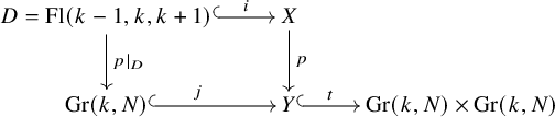
where the left square is a fibered product and
 $t \circ j=\Delta $
is the diagonal map.
$t \circ j=\Delta $
is the diagonal map.
Since
 $t_*$
is exact and
$t_*$
is exact and
 $\Delta _*=t_*j_*$
, it is equivalent to show
$\Delta _*=t_*j_*$
, it is equivalent to show
 $p_*(\mathcal {O}_{2D} \otimes (\mathcal {V}'/\mathcal {V})^{\otimes (N-k+1)})$
is neither isomorphic to
$p_*(\mathcal {O}_{2D} \otimes (\mathcal {V}'/\mathcal {V})^{\otimes (N-k+1)})$
is neither isomorphic to
 $j_{*}\Bigl (\mathbb {C}^N\otimes \det (\mathbb {C}^N/\mathcal {V})\Bigr )[1+k-N]$
nor to
$j_{*}\Bigl (\mathbb {C}^N\otimes \det (\mathbb {C}^N/\mathcal {V})\Bigr )[1+k-N]$
nor to
 $j_*\Bigl ((\mathcal {V} \oplus \mathbb {C}^N/\mathcal {V}) \otimes \det (\mathbb {C}^N/\mathcal {V})\Bigr )[1+k-N]$
.
$j_*\Bigl ((\mathcal {V} \oplus \mathbb {C}^N/\mathcal {V}) \otimes \det (\mathbb {C}^N/\mathcal {V})\Bigr )[1+k-N]$
.
Assume otherwise, then applying
 $j^*$
we have
$j^*$
we have
 $$ \begin{align} j^*p_*(\mathcal{O}_{2D} \otimes (\mathcal{V}'/\mathcal{V})^{\otimes (N-k+1)}) &\cong j^*j_{*}\Bigl(\mathbb{C}^N\otimes \det(\mathbb{C}^N/\mathcal{V})\Bigr)[1+k-N] \nonumber \\ &\mathrm{or} \ j^*j_*\Bigl((\mathcal{V} \oplus \mathbb{C}^N/\mathcal{V}) \otimes \det(\mathbb{C}^N/\mathcal{V})\Bigr)[1+k-N]. \end{align} $$
Taking the sheaf cohomology
 $\mathcal {H}^l$
to both sides of (6.17), by Lemma 4.6, we obtain
$\mathcal {H}^l$
to both sides of (6.17), by Lemma 4.6, we obtain
 $$ \begin{align} \mathcal{H}^l(j^*p_*(\mathcal{O}_{2D} \otimes (\mathcal{V}'/\mathcal{V})^{\otimes (N-k+1)}) ) &\cong \bigoplus_{s-r=l} \bigwedge^{r} \mathcal{N}^{\vee}_{j} \otimes \mathcal{H}^s(\mathbb{C}^N\otimes \det(\mathbb{C}^N/\mathcal{V})[1+k-N])\end{align} $$
 $$ \begin{align} &\mathrm{or} \ \bigoplus_{s-r=l} \bigwedge^{r} \mathcal{N}^{\vee}_{j} \otimes \mathcal{H}^s((\mathcal{V} \oplus \mathbb{C}^N/\mathcal{V})\otimes \det(\mathbb{C}^N/\mathcal{V})[1+k-N]). \end{align} $$
Since
 $\mathbb {C}^N\otimes \det (\mathbb {C}^N/\mathcal {V})[1+k-N]$
and
$\mathbb {C}^N\otimes \det (\mathbb {C}^N/\mathcal {V})[1+k-N]$
and
 $(\mathcal {V} \oplus \mathbb {C}^N/\mathcal {V})\otimes \det (\mathbb {C}^N/\mathcal {V})[1+k-N]$
are complex concentrate at degree
$(\mathcal {V} \oplus \mathbb {C}^N/\mathcal {V})\otimes \det (\mathbb {C}^N/\mathcal {V})[1+k-N]$
are complex concentrate at degree
 $N-k-1$
, the only value s such that
$N-k-1$
, the only value s such that
 $\mathcal {H}^s \neq 0$
in (6.18) and (6.19) is
$\mathcal {H}^s \neq 0$
in (6.18) and (6.19) is
 $s=N-k-1$
. Thus, if we choose
$s=N-k-1$
. Thus, if we choose
 $l=N-k-1$
, then
$l=N-k-1$
, then
 $r=s-l=0$
and
$r=s-l=0$
and
 $$ \begin{align} \mathcal{H}^{N-k-1}(j^*p_*(\mathcal{O}_{2D} \otimes (\mathcal{V}'/\mathcal{V})^{\otimes (N-k+1)}) ) \cong \mathbb{C}^N \otimes \det(\mathbb{C}^N/\mathcal{V}) \ \mathrm{or} \ (\mathcal{V} \oplus \mathbb{C}^N/\mathcal{V})\otimes \det(\mathbb{C}^N/\mathcal{V}). \end{align} $$
On the other hand, using base change, the left-hand side of (6.17) becomes
 $$ \begin{align*} j^*p_{*}(\mathcal{O}_{2D} \otimes (\mathcal{V}'/\mathcal{V})^{\otimes (N-k+1)}) \cong p|_{D*}i^*(\mathcal{O}_{2D} \otimes (\mathcal{V}'/\mathcal{V})^{\otimes (N-k+1)}). \end{align*} $$
We tensor (5.16) with
 $n=2$
by
$n=2$
by
 $(\mathcal {V}'/\mathcal {V})^{\otimes (N-k-1)}$
such that it becomes
$(\mathcal {V}'/\mathcal {V})^{\otimes (N-k-1)}$
such that it becomes
 $$ \begin{align*} (\mathcal{V}"/\mathcal{V}"')^{\otimes 2} \otimes (\mathcal{V}'/\mathcal{V})^{\otimes (N-k-1)} \xrightarrow{c\otimes id} (\mathcal{V}'/\mathcal{V})^{\otimes (N-k+1)} \rightarrow \mathcal{O}_{2D} \otimes (\mathcal{V}'/\mathcal{V})^{\otimes (N-k+1)} \end{align*} $$
where we denote
 $c:(\mathcal {V}"/\mathcal {V}"')^{\otimes 2} \rightarrow (\mathcal {V}'/\mathcal {V})^{\otimes 2}$
to be the natural inclusion. Applying the pullback
$c:(\mathcal {V}"/\mathcal {V}"')^{\otimes 2} \rightarrow (\mathcal {V}'/\mathcal {V})^{\otimes 2}$
to be the natural inclusion. Applying the pullback
 $i^*$
, since we have
$i^*$
, since we have
 $V=V"$
on D, the map c becomes
$V=V"$
on D, the map c becomes
 $0$
and thus
$0$
and thus
 $$ \begin{align*} i^*((\mathcal{V}"/\mathcal{V}"')^{\otimes 2} \otimes (\mathcal{V}'/\mathcal{V})^{\otimes (N-k-1)}) \xrightarrow{0} i^*((\mathcal{V}'/\mathcal{V})^{\otimes (N-k+1)}) \rightarrow i^*(\mathcal{O}_{2D} \otimes (\mathcal{V}'/\mathcal{V})^{\otimes (N-k+1)}), \end{align*} $$
which is again an exact triangle. Thus,
 $$ \begin{align*} i^*(\mathcal{O}_{2D} \otimes (\mathcal{V}'/\mathcal{V})^{\otimes (N-k+1)}) \cong i^*((\mathcal{V}"/\mathcal{V}"')^{\otimes 2} \otimes (\mathcal{V}'/\mathcal{V})^{\otimes (N-k-1)}) [1] \bigoplus i^*((\mathcal{V}'/\mathcal{V})^{\otimes (N-k+1)}). \end{align*} $$
Using projection formula and Proposition 4.4, we conclude that
 $$ \begin{align*} p|_{D*}i^*(\mathcal{O}_{2D} \otimes (\mathcal{V}'/\mathcal{V})^{\otimes (N-k+1)}) \cong \mathbb{C}^N/\mathcal{V} \otimes \det(\mathbb{C}^N/V) [1+k-N]. \end{align*} $$
When
 $l=N-k-1$
,
$l=N-k-1$
,
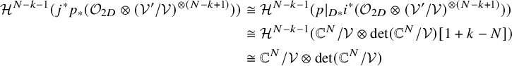 $$ \begin{align*} \mathcal{H}^{N-k-1}(j^*p_{*}(\mathcal{O}_{2D} \otimes (\mathcal{V}'/\mathcal{V})^{\otimes (N-k+1)})) &\cong \mathcal{H}^{N-k-1}(p|_{D*}i^*(\mathcal{O}_{2D} \otimes (\mathcal{V}'/\mathcal{V})^{\otimes (N-k+1)})) \\ & \cong \mathcal{H}^{N-k-1}(\mathbb{C}^N/\mathcal{V} \otimes \det(\mathbb{C}^N/\mathcal{V}) [1+k-N]) \\ & \cong \mathbb{C}^N/\mathcal{V} \otimes \det(\mathbb{C}^N/\mathcal{V}) \end{align*} $$
which is not isomorphic to (6.20). Hence, we obtain a contradiction.
Remark 6.3. A similar argument shows that
 $\mathcal {H}_{-1}\boldsymbol {1}_{(k,N-k)}$
is neither isomorphic to
$\mathcal {H}_{-1}\boldsymbol {1}_{(k,N-k)}$
is neither isomorphic to
 $\Delta _{*}(\mathbb {C}^N)^{\vee }$
nor to
$\Delta _{*}(\mathbb {C}^N)^{\vee }$
nor to
 $\Delta _*(\mathcal {V}^{\vee } \oplus (\mathbb {C}^N/\mathcal {V})^{\vee })$
.
$\Delta _*(\mathcal {V}^{\vee } \oplus (\mathbb {C}^N/\mathcal {V})^{\vee })$
.
6.3 Calculation of Convolutions and a Conjecture
Although the application of
 $\mathsf {{H}}_{\pm 1}\boldsymbol {1}_{(k,N-k)}$
is unclear to us, it is still interesting to know the categorical commutator relations between
$\mathsf {{H}}_{\pm 1}\boldsymbol {1}_{(k,N-k)}$
is unclear to us, it is still interesting to know the categorical commutator relations between
 $\mathsf {{H}}_{\pm 1}\boldsymbol {1}_{(k,N-k)}$
and other 1-morphisms.
$\mathsf {{H}}_{\pm 1}\boldsymbol {1}_{(k,N-k)}$
and other 1-morphisms.
We will only consider the relations between
 $\mathsf {{H}}_1\boldsymbol {1}_{(k,N-k)}$
and
$\mathsf {{H}}_1\boldsymbol {1}_{(k,N-k)}$
and
 $\mathsf {\Psi }^{+}\boldsymbol {1}_{(k,N-k)}$
,
$\mathsf {\Psi }^{+}\boldsymbol {1}_{(k,N-k)}$
,
 $\mathsf {E}_r\boldsymbol {1}_{(k,N-k)}$
since the arguments for the others are similar. Then we have to calculate the convolutions of the FM kernels between
$\mathsf {E}_r\boldsymbol {1}_{(k,N-k)}$
since the arguments for the others are similar. Then we have to calculate the convolutions of the FM kernels between
 $\mathcal {H}_{1}\boldsymbol {1}_{(k,N-k)}$
and
$\mathcal {H}_{1}\boldsymbol {1}_{(k,N-k)}$
and
 $\Psi ^{+}\boldsymbol {1}_{(k,N-k)}$
,
$\Psi ^{+}\boldsymbol {1}_{(k,N-k)}$
,
 $\mathcal {E}_{r}\boldsymbol {1}_{(k,N-k)}$
.
$\mathcal {E}_{r}\boldsymbol {1}_{(k,N-k)}$
.
By Proposition 6.2, the kernel
 $\mathcal {H}_1\boldsymbol {1}_{(k,N-k)}$
is complicated. Thus, the computation of convolutions involving
$\mathcal {H}_1\boldsymbol {1}_{(k,N-k)}$
is complicated. Thus, the computation of convolutions involving
 $\mathcal {H}_1\boldsymbol {1}_{(k,N-k)}$
is generally difficult to carry out. In this subsection, we provide the calculation in the simplest case
$\mathcal {H}_1\boldsymbol {1}_{(k,N-k)}$
is generally difficult to carry out. In this subsection, we provide the calculation in the simplest case
 $N=2$
.
$N=2$
.
When
 $N=2$
,
$N=2$
,
 $\mathrm {Gr}(0,2)=\mathrm {Gr}(2,2)=pt$
and
$\mathrm {Gr}(0,2)=\mathrm {Gr}(2,2)=pt$
and
 $\mathrm {Gr}(1,2)=\mathbb {P}^1$
. The most interesting case is when
$\mathrm {Gr}(1,2)=\mathbb {P}^1$
. The most interesting case is when
 $k=1$
where the fibered product variety X in (5.3) is given by
$k=1$
where the fibered product variety X in (5.3) is given by
 $$ \begin{align*} X=\{(0,V,V",\mathbb{C}^2) \in \mathrm{Gr}(0,2) \times \mathbb{P}^1 \times \mathbb{P}^1 \times \mathrm{Gr}(2,2) \ | \ 0 \subset V \subset \mathbb{C}^2, \ 0 \subset V" \subset \mathbb{C}^2 \} \end{align*} $$
and similarly the variety Y from diagram (5.1) is given by
 $$ \begin{align*} Y=\{(V,V") \in \mathbb{P}^1 \times \mathbb{P}^1 \ | \ \dim(V \cap V") \geq 0 \}. \end{align*} $$
Thus we obtain
 $X=Y=\mathbb {P}^1 \times \mathbb {P}^1$
. Both the projection map
$X=Y=\mathbb {P}^1 \times \mathbb {P}^1$
. Both the projection map
 $p:X \rightarrow Y$
and the inclusion map
$p:X \rightarrow Y$
and the inclusion map
 $t: Y \rightarrow \mathbb {P}^1 \times \mathbb {P}^1$
are the identity map. Let
$t: Y \rightarrow \mathbb {P}^1 \times \mathbb {P}^1$
are the identity map. Let
 $\pi _{i}:\mathbb {P}^1 \times \mathbb {P}^1 \rightarrow \mathbb {P}^1$
be the natural projection to the i-th copy where
$\pi _{i}:\mathbb {P}^1 \times \mathbb {P}^1 \rightarrow \mathbb {P}^1$
be the natural projection to the i-th copy where
 $i=1,2$
. We also denote
$i=1,2$
. We also denote
 $\mathcal {V}$
and
$\mathcal {V}$
and
 $\mathcal {V}"$
as the two tautological line bundles on the first and second copies of
$\mathcal {V}"$
as the two tautological line bundles on the first and second copies of
 $\mathbb {P}^1$
. Then we have the two tautological line bundles
$\mathbb {P}^1$
. Then we have the two tautological line bundles
 $\pi ^*_{1}\mathcal {V}$
,
$\pi ^*_{1}\mathcal {V}$
,
 $\pi ^*_{2}\mathcal {V}"$
on
$\pi ^*_{2}\mathcal {V}"$
on
 $\mathbb {P}^1 \times \mathbb {P}^1$
. Let
$\mathbb {P}^1 \times \mathbb {P}^1$
. Let
 $\mathbb {C}^2$
be the trivial bundle of rank two on
$\mathbb {C}^2$
be the trivial bundle of rank two on
 $\mathbb {P}^1$
and denote
$\mathbb {P}^1$
and denote
 $\Delta : \mathbb {P}^1 \rightarrow \mathbb {P}^1 \times \mathbb {P}^1$
as the diagonal map. By abusing notations, we still denote its image as
$\Delta : \mathbb {P}^1 \rightarrow \mathbb {P}^1 \times \mathbb {P}^1$
as the diagonal map. By abusing notations, we still denote its image as
 $\Delta $
. Then the associated line bundle is
$\Delta $
. Then the associated line bundle is
 $\mathcal {O}_{\mathbb {P}^1 \times \mathbb {P}^1}(-\Delta ) = \pi ^*_{2}\mathcal {V}" \otimes \pi ^*_{1}(\mathbb {C}^2/\mathcal {V})^{-1}$
. Then, from (6.7), we have
$\mathcal {O}_{\mathbb {P}^1 \times \mathbb {P}^1}(-\Delta ) = \pi ^*_{2}\mathcal {V}" \otimes \pi ^*_{1}(\mathbb {C}^2/\mathcal {V})^{-1}$
. Then, from (6.7), we have
 $\mathcal {H}_1\boldsymbol {1}_{(1,1)}=\mathcal {O}_{2\Delta } \otimes \pi ^*_1(\mathbb {C}^2/\mathcal {V})^{\otimes 2} \otimes \pi ^*_2(\mathbb {C}^2/\mathcal {V}")^{-1}$
.
$\mathcal {H}_1\boldsymbol {1}_{(1,1)}=\mathcal {O}_{2\Delta } \otimes \pi ^*_1(\mathbb {C}^2/\mathcal {V})^{\otimes 2} \otimes \pi ^*_2(\mathbb {C}^2/\mathcal {V}")^{-1}$
.
First, we compute the convolutions between
 $\mathcal {H}_1\boldsymbol {1}_{(1,1)}$
and
$\mathcal {H}_1\boldsymbol {1}_{(1,1)}$
and
 $\Psi ^+\boldsymbol {1}_{(1,1)}$
and show that they are non-isomorphic.
$\Psi ^+\boldsymbol {1}_{(1,1)}$
and show that they are non-isomorphic.
Proposition 6.4.
 $(\Psi ^{+} \ast \mathcal {H}_1)\boldsymbol {1}_{(1,1)} \ncong (\mathcal {H}_1 \ast \Psi ^{+}) \boldsymbol {1}_{(1,1)}$
.
$(\Psi ^{+} \ast \mathcal {H}_1)\boldsymbol {1}_{(1,1)} \ncong (\mathcal {H}_1 \ast \Psi ^{+}) \boldsymbol {1}_{(1,1)}$
.
Proof. It is standard to check that
 $(\Psi ^{+} \ast \mathcal {H}_1) \boldsymbol {1}_{(1,1)}=\mathcal {O}_{2\Delta } \otimes \pi ^*_{1}(\mathbb {C}^2/\mathcal {V})^{\otimes 2}$
. Now, we calculate
$(\Psi ^{+} \ast \mathcal {H}_1) \boldsymbol {1}_{(1,1)}=\mathcal {O}_{2\Delta } \otimes \pi ^*_{1}(\mathbb {C}^2/\mathcal {V})^{\otimes 2}$
. Now, we calculate
 $(\mathcal {H}_1 \ast \Psi ^{+}) \boldsymbol {1}_{(1,1)}$
. Using base-change with respect to
$(\mathcal {H}_1 \ast \Psi ^{+}) \boldsymbol {1}_{(1,1)}$
. Using base-change with respect to
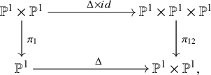
we have
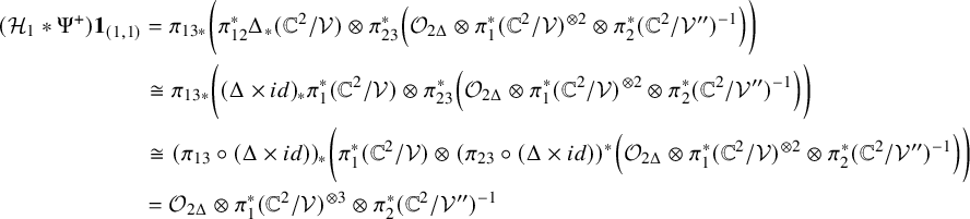 $$ \begin{align*} (\mathcal{H}_1 \ast \Psi^{+}) \boldsymbol{1}_{(1,1)} &= \pi_{13*}\biggl(\pi^*_{12}\Delta_{*}(\mathbb{C}^2/\mathcal{V}) \otimes \pi^*_{23}\Bigl(\mathcal{O}_{2\Delta} \otimes \pi^*_{1}(\mathbb{C}^2/\mathcal{V})^{\otimes 2} \otimes \pi^*_{2}(\mathbb{C}^2/\mathcal{V}")^{-1} \Bigr) \biggr) \\ &\cong \pi_{13*}\biggl((\Delta \times id)_{*}\pi^*_{1}(\mathbb{C}^2/\mathcal{V}) \otimes \pi^*_{23}\Bigl(\mathcal{O}_{2\Delta} \otimes \pi^*_{1}(\mathbb{C}^2/\mathcal{V})^{\otimes 2} \otimes \pi^*_{2}(\mathbb{C}^2/\mathcal{V}")^{-1} \Bigr)\biggr) \\ &\cong (\pi_{13} \circ (\Delta \times id))_{*} \biggl( \pi^*_{1}(\mathbb{C}^2/\mathcal{V}) \otimes (\pi_{23} \circ (\Delta \times id))^{*}\Bigl(\mathcal{O}_{2\Delta} \otimes \pi^*_{1}(\mathbb{C}^2/\mathcal{V})^{\otimes 2} \otimes \pi^*_{2}(\mathbb{C}^2/\mathcal{V}")^{-1} \Bigr ) \biggr) \\ & = \mathcal{O}_{2\Delta} \otimes \pi^*_{1}(\mathbb{C}^2/\mathcal{V})^{\otimes 3} \otimes \pi^*_{2}(\mathbb{C}^2/\mathcal{V}")^{-1} \end{align*} $$
since
 $\pi _{13} \circ (\Delta \times id)=id$
,
$\pi _{13} \circ (\Delta \times id)=id$
,
 $\pi _{23} \circ (\Delta \times id)=id$
.
$\pi _{23} \circ (\Delta \times id)=id$
.
To see that
 $(\Psi ^{+} \ast \mathcal {H}_1) \boldsymbol {1}_{(1,1)} \ncong (\mathcal {H}_1 \ast \Psi ^{+}) \boldsymbol {1}_{(1,1)}$
, we apply the pushforward
$(\Psi ^{+} \ast \mathcal {H}_1) \boldsymbol {1}_{(1,1)} \ncong (\mathcal {H}_1 \ast \Psi ^{+}) \boldsymbol {1}_{(1,1)}$
, we apply the pushforward
 $\pi _{1*}$
to them and using the projection formula we obtain
$\pi _{1*}$
to them and using the projection formula we obtain
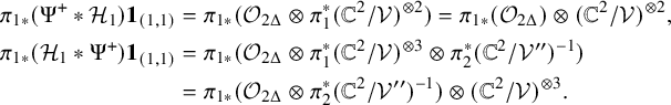 $$ \begin{align*} \pi_{1*}(\Psi^{+} \ast \mathcal{H}_{1}) \boldsymbol{1}_{(1,1)} &= \pi_{1*}(\mathcal{O}_{2\Delta} \otimes \pi^*_{1}(\mathbb{C}^2/\mathcal{V})^{\otimes 2}) = \pi_{1*}(\mathcal{O}_{2\Delta}) \otimes (\mathbb{C}^2/\mathcal{V})^{\otimes 2}, \\ \pi_{1*}(\mathcal{H}_1 \ast \Psi^{+}) \boldsymbol{1}_{(1,1)} &= \pi_{1*}(\mathcal{O}_{2\Delta} \otimes \pi^*_{1}(\mathbb{C}^2/\mathcal{V})^{\otimes 3} \otimes \pi^*_{2}(\mathbb{C}^2/\mathcal{V}")^{-1}) \\ &=\pi_{1*}(\mathcal{O}_{2\Delta} \otimes \pi^*_{2}(\mathbb{C}^2/\mathcal{V}")^{-1}) \otimes (\mathbb{C}^2/\mathcal{V})^{\otimes 3}. \end{align*} $$
To calculate
 $\pi _{1*}(\mathcal {O}_{2\Delta })$
, we use the following exact triangle
$\pi _{1*}(\mathcal {O}_{2\Delta })$
, we use the following exact triangle
 $$ \begin{align} \mathcal{O}_{\mathbb{P}^1 \times \mathbb{P}^1}(-2\Delta) \rightarrow \mathcal{O}_{\mathbb{P}^1 \times \mathbb{P}^1} \rightarrow \mathcal{O}_{2\Delta}. \end{align} $$
Note that
 $\mathcal {O}_{\mathbb {P}^1 \times \mathbb {P}^1}(-\Delta ) = \pi ^*_{2}\mathcal {V}" \otimes \pi ^*_{1}(\mathbb {C}^2/\mathcal {V})^{-1}$
, thus
$\mathcal {O}_{\mathbb {P}^1 \times \mathbb {P}^1}(-\Delta ) = \pi ^*_{2}\mathcal {V}" \otimes \pi ^*_{1}(\mathbb {C}^2/\mathcal {V})^{-1}$
, thus
 $$ \begin{align*} \pi_{1*}\mathcal{O}_{\mathbb{P}^1 \times \mathbb{P}^1}(-2\Delta)=\pi_{1*}(\pi^*_{2}(\mathcal{V}")^{\otimes 2} \otimes \pi^*_{1}(\mathbb{C}^2/\mathcal{V})^{\otimes (-2)}) \cong \pi_{1*}\pi^*_{2}(\mathcal{V}")^{\otimes 2} \otimes (\mathbb{C}^2/\mathcal{V})^{\otimes (-2)} \cong (\mathbb{C}^2/\mathcal{V})^{\otimes (-2)}[-1] \end{align*} $$
since
 $H^*(\mathbb {P}^1,\mathcal {O}_{\mathbb {P}^1}(-2))=\mathbb {C}[-1]$
. Then, after applying
$H^*(\mathbb {P}^1,\mathcal {O}_{\mathbb {P}^1}(-2))=\mathbb {C}[-1]$
. Then, after applying
 $\pi _{1*}$
to (6.21), it becomes
$\pi _{1*}$
to (6.21), it becomes
 $$ \begin{align} \mathcal{O}_{\mathbb{P}^1} \rightarrow \pi_{1*}\mathcal{O}_{2\Delta} \rightarrow (\mathbb{C}^2/\mathcal{V})^{\otimes (-2)} \end{align} $$
and
 $\pi _{1*}(\mathcal {O}_{2\Delta })$
is determined by
$\pi _{1*}(\mathcal {O}_{2\Delta })$
is determined by
 $\mathrm {Ext}^1((\mathbb {C}^2/\mathcal {V})^{\otimes (-2)}, \mathcal {O}_{\mathbb {P}^1})=\mathrm {Ext}^1(\mathcal {O}_{\mathbb {P}^1}(-2), \mathcal {O}_{\mathbb {P}^1})=H^1(\mathbb {P}^1,\mathcal {O}_{\mathbb {P}^1}(2))=0$
.
$\mathrm {Ext}^1((\mathbb {C}^2/\mathcal {V})^{\otimes (-2)}, \mathcal {O}_{\mathbb {P}^1})=\mathrm {Ext}^1(\mathcal {O}_{\mathbb {P}^1}(-2), \mathcal {O}_{\mathbb {P}^1})=H^1(\mathbb {P}^1,\mathcal {O}_{\mathbb {P}^1}(2))=0$
.
Thus
 $$ \begin{align*} \pi_{1*}(\mathcal{O}_{2\Delta})=(\mathbb{C}^2/\mathcal{V})^{\otimes (-2)} \oplus \mathcal{O}_{\mathbb{P}^1} \end{align*} $$
and we obtain
 $$ \begin{align} \pi_{1*}(\Psi^{+} \ast \mathcal{H}_{1}) \boldsymbol{1}_{(1,1)} = \pi_{1*}(\mathcal{O}_{2\Delta}) \otimes (\mathbb{C}^2/\mathcal{V})^{\otimes 2} =(\mathbb{C}^2/\mathcal{V})^{\otimes 2} \oplus \mathcal{O}_{\mathbb{P}^1} = \mathcal{O}_{\mathbb{P}^1}(2) \oplus \mathcal{O}_{\mathbb{P}^1}. \end{align} $$
On the other hand, to calculate
 $\pi _{1*}(\mathcal {O}_{2\Delta } \otimes \pi ^*_{2}(\mathbb {C}^2/\mathcal {V}")^{-1})$
, we tensor (6.21) with
$\pi _{1*}(\mathcal {O}_{2\Delta } \otimes \pi ^*_{2}(\mathbb {C}^2/\mathcal {V}")^{-1})$
, we tensor (6.21) with
 $\pi ^*_{2}(\mathbb {C}^2/\mathcal {V}")^{-1}$
to get
$\pi ^*_{2}(\mathbb {C}^2/\mathcal {V}")^{-1}$
to get
 $$ \begin{align*} \mathcal{O}_{\mathbb{P}^1 \times \mathbb{P}^1}(-2\Delta)\otimes \pi^*_{2}(\mathbb{C}^2/\mathcal{V}")^{-1} \rightarrow \pi^*_{2}(\mathbb{C}^2/\mathcal{V}")^{-1} \rightarrow \mathcal{O}_{2\Delta}\otimes \pi^*_{2}(\mathbb{C}^2/\mathcal{V}")^{-1}. \end{align*} $$
Then, applying
 $\pi _{1*}$
, we calculate
$\pi _{1*}$
, we calculate
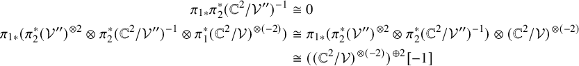 $$ \begin{align*} \pi_{1*}\pi^*_{2}(\mathbb{C}^2/\mathcal{V}")^{-1} &\cong 0 \\ \pi_{1*}(\pi^*_{2}(\mathcal{V}")^{\otimes 2} \otimes \pi^*_{2}(\mathbb{C}^2/\mathcal{V}")^{-1} \otimes \pi^*_{1}(\mathbb{C}^2/\mathcal{V})^{\otimes (-2)}) &\cong \pi_{1*}(\pi^*_{2}(\mathcal{V}")^{\otimes 2} \otimes \pi^*_{2}(\mathbb{C}^2/\mathcal{V}")^{-1}) \otimes (\mathbb{C}^2/\mathcal{V})^{\otimes (-2)} \\ &\cong ((\mathbb{C}^2/\mathcal{V})^{\otimes (-2)})^{\oplus 2}[-1] \end{align*} $$
since
 $H^*(\mathbb {P}^1,\mathcal {O}_{\mathbb {P}^1}(-1))=0$
and
$H^*(\mathbb {P}^1,\mathcal {O}_{\mathbb {P}^1}(-1))=0$
and
 $H^*(\mathbb {P}^1,\mathcal {O}_{\mathbb {P}^1}(-3))=\mathbb {C}^2[-1]$
.
$H^*(\mathbb {P}^1,\mathcal {O}_{\mathbb {P}^1}(-3))=\mathbb {C}^2[-1]$
.
Thus,
 $$ \begin{align} \pi_{1*}(\mathcal{O}_{2\Delta}\otimes \pi^*_{2}(\mathbb{C}^2/\mathcal{V}")^{-1})= ((\mathbb{C}^2/\mathcal{V})^{\otimes (-2)})^{\oplus 2} \end{align} $$
which implies
 $$ \begin{align} \pi_{1*}(\mathcal{H}_1 \ast \Psi^{+}) \boldsymbol{1}_{(1,1)} =\pi_{1*}(\mathcal{O}_{2\Delta} \otimes \pi^*_{2}(\mathbb{C}^2/\mathcal{V}")^{-1}) \otimes (\mathbb{C}^2/\mathcal{V})^{\otimes 3} =(\mathbb{C}^2/\mathcal{V})^{\oplus 2}=\mathcal{O}_{\mathbb{P}^1}(1)^{\oplus 2} \end{align} $$
which is not isomorphic to (6.23).
Remark 6.5. Using the same argument, we can also show that
 $(\mathcal {H}_1 \ast \Psi ^{-}) \boldsymbol {1}_{(1,1)} \ncong (\Psi ^{-} \ast \mathcal {H}_1) \boldsymbol {1}_{(1,1)}$
.
$(\mathcal {H}_1 \ast \Psi ^{-}) \boldsymbol {1}_{(1,1)} \ncong (\Psi ^{-} \ast \mathcal {H}_1) \boldsymbol {1}_{(1,1)}$
.
Next, we compute the convolutions between
 $\mathcal {H}_1\boldsymbol {1}_{(1,1)}$
and
$\mathcal {H}_1\boldsymbol {1}_{(1,1)}$
and
 $\mathcal {E}_{r}\boldsymbol {1}_{(1,1)}$
. Note that besides
$\mathcal {E}_{r}\boldsymbol {1}_{(1,1)}$
. Note that besides
 $r=-1,-0$
, we also have the FM kernel
$r=-1,-0$
, we also have the FM kernel
 $\mathcal {E}_{-2}\boldsymbol {1}_{(1,1)}$
since we have defined the new 1-morphism
$\mathcal {E}_{-2}\boldsymbol {1}_{(1,1)}$
since we have defined the new 1-morphism
 $\mathsf {E}_{-2}\boldsymbol {1}_{(1,1)}$
.
$\mathsf {E}_{-2}\boldsymbol {1}_{(1,1)}$
.
Proposition 6.6. We have the following exact triangle in
 $\mathrm {D}^b(\mathrm {Gr}(1,2) \times \mathrm {Gr}(0,2))=\mathrm {D}^b(\mathbb {P}^1)$
 $$ \begin{align*} (\mathcal{H}_{1} \ast \mathcal{E}_{-1})\boldsymbol{1}_{(1,1)} \rightarrow (\mathcal{E}_{-1} \ast \mathcal{H}_1)\boldsymbol{1}_{(1,1)} \rightarrow \mathcal{E}_{0}\boldsymbol{1}_{(1,1)} \oplus \mathcal{E}_{0}\boldsymbol{1}_{(1,1)}[1] \end{align*} $$
and
 $(\mathcal {H}_{1} \ast \mathcal {E}_{0})\boldsymbol {1}_{(1,1)} \cong (\mathcal {E}_{0} \ast \mathcal {H}_1)\boldsymbol {1}_{(1,1)}$
,
$(\mathcal {H}_{1} \ast \mathcal {E}_{0})\boldsymbol {1}_{(1,1)} \cong (\mathcal {E}_{0} \ast \mathcal {H}_1)\boldsymbol {1}_{(1,1)}$
,
 $(\mathcal {H}_{1} \ast \mathcal {E}_{-2})\boldsymbol {1}_{(1,1)} \cong (\mathcal {E}_{-2} \ast \mathcal {H}_1)\boldsymbol {1}_{(1,1)}$
.
$(\mathcal {H}_{1} \ast \mathcal {E}_{-2})\boldsymbol {1}_{(1,1)} \cong (\mathcal {E}_{-2} \ast \mathcal {H}_1)\boldsymbol {1}_{(1,1)}$
.
Proof. First, we calculate
 $(\mathcal {H}_1 \ast \mathcal {E}_{r}) \boldsymbol {1}_{(1,1)}$
. To know
$(\mathcal {H}_1 \ast \mathcal {E}_{r}) \boldsymbol {1}_{(1,1)}$
. To know
 $\mathcal {H}_{1}\boldsymbol {1}_{(0,2)}$
, from Proposition 5.10, we have the following exact triangle
$\mathcal {H}_{1}\boldsymbol {1}_{(0,2)}$
, from Proposition 5.10, we have the following exact triangle
 $$ \begin{align*} (\mathcal{F}_{3} \ast \mathcal{E}_{0}) \boldsymbol{1}_{(0,2)} \rightarrow (\mathcal{E}_{0} \ast \mathcal{F}_{3})\boldsymbol{1}_{(0,2)} \rightarrow (\Psi^{+} \ast \mathcal{H}_{1})\boldsymbol{1}_{(0,2)}. \end{align*} $$
Since
 $(\mathcal {F}_{3} \ast \mathcal {E}_{0}) \boldsymbol {1}_{(0,2)}=0$
and
$(\mathcal {F}_{3} \ast \mathcal {E}_{0}) \boldsymbol {1}_{(0,2)}=0$
and
 $\Psi ^{+}\boldsymbol {1}_{(0,2)}=\Delta _{*}\mathbb {C}[-1] \in \mathrm {D}^b(\mathrm {Gr}(0,2) \times \mathrm {Gr}(0,2))$
, a direct calculation shows that
$\Psi ^{+}\boldsymbol {1}_{(0,2)}=\Delta _{*}\mathbb {C}[-1] \in \mathrm {D}^b(\mathrm {Gr}(0,2) \times \mathrm {Gr}(0,2))$
, a direct calculation shows that
 $(\mathcal {E}_{0} \ast \mathcal {F}_{3})\boldsymbol {1}_{(0,2)} \cong \mathbb {C}^2[-1] \in \mathrm {D}^b(\mathrm {Gr}(0,2) \times \mathrm {Gr}(0,2))$
.
$(\mathcal {E}_{0} \ast \mathcal {F}_{3})\boldsymbol {1}_{(0,2)} \cong \mathbb {C}^2[-1] \in \mathrm {D}^b(\mathrm {Gr}(0,2) \times \mathrm {Gr}(0,2))$
.
So,
 $\mathcal {H}_{1}\boldsymbol {1}_{(0,2)}=((\Psi ^{+})^{-1} \ast \mathcal {E}_{0} \ast \mathcal {F}_{3})\boldsymbol {1}_{(0,2)} \cong \mathbb {C}^2$
, and
$\mathcal {H}_{1}\boldsymbol {1}_{(0,2)}=((\Psi ^{+})^{-1} \ast \mathcal {E}_{0} \ast \mathcal {F}_{3})\boldsymbol {1}_{(0,2)} \cong \mathbb {C}^2$
, and
 $(\mathcal {H}_1 \ast \mathcal {E}_{r}) \boldsymbol {1}_{(1,1)} = \mathcal {O}_{\mathbb {P}^1}(-r)^{\oplus 2}$
since
$(\mathcal {H}_1 \ast \mathcal {E}_{r}) \boldsymbol {1}_{(1,1)} = \mathcal {O}_{\mathbb {P}^1}(-r)^{\oplus 2}$
since
 $\pi _{12}=\pi _{23}=\pi _{13}=id$
.
$\pi _{12}=\pi _{23}=\pi _{13}=id$
.
Next, we calculate
 $(\mathcal {E}_{r} \ast \mathcal {H}_{1}) \boldsymbol {1}_{(1,1)}$
, which is given by
$(\mathcal {E}_{r} \ast \mathcal {H}_{1}) \boldsymbol {1}_{(1,1)}$
, which is given by
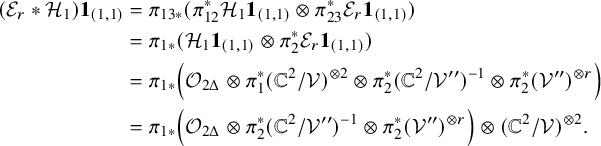 $$ \begin{align*} (\mathcal{E}_{r} \ast \mathcal{H}_{1}) \boldsymbol{1}_{(1,1)} &= \pi_{13*}(\pi^*_{12}\mathcal{H}_{1}\boldsymbol{1}_{(1,1)} \otimes \pi^*_{23}\mathcal{E}_{r}\boldsymbol{1}_{(1,1)}) \\ &= \pi_{1*}(\mathcal{H}_{1}\boldsymbol{1}_{(1,1)} \otimes \pi^*_{2}\mathcal{E}_{r}\boldsymbol{1}_{(1,1)}) \\ &= \pi_{1*}\Bigl(\mathcal{O}_{2\Delta} \otimes \pi^*_{1}(\mathbb{C}^2/\mathcal{V})^{\otimes 2} \otimes \pi^*_{2}(\mathbb{C}^2/\mathcal{V}")^{-1} \otimes \pi^*_{2}(\mathcal{V}")^{\otimes r}\Bigr) \\ &= \pi_{1*}\Bigl(\mathcal{O}_{2\Delta} \otimes \pi^*_{2}(\mathbb{C}^2/\mathcal{V}")^{-1} \otimes \pi^*_{2}(\mathcal{V}")^{\otimes r} \Bigr ) \otimes (\mathbb{C}^2/\mathcal{V})^{\otimes 2}. \end{align*} $$
From (6.3) and (6.24), we know that
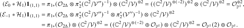 $$ \begin{align*} (\mathcal{E}_{0} \ast \mathcal{H}_{1}) \boldsymbol{1}_{(1,1)} &=\pi_{1*}(\mathcal{O}_{2\Delta} \otimes \pi^*_{2}(\mathbb{C}^2/\mathcal{V}")^{-1}) \otimes (\mathbb{C}^2/\mathcal{V})^{\otimes 2} = ((\mathbb{C}^2/\mathcal{V})^{\otimes (-2)})^{\oplus 2} \otimes (\mathbb{C}^2/\mathcal{V})^{\otimes 2} = \mathcal{O}_{\mathbb{P}^1}^{\oplus 2},\\(\mathcal{E}_{-1} \ast \mathcal{H}_{1}) \boldsymbol{1}_{(1,1)} &=\pi_{1*}(\mathcal{O}_{2\Delta} \otimes \pi^*_{2}(\mathbb{C}^2/\mathcal{V}")^{-1} \otimes \pi^*_{2}(\mathcal{V}")^{-1}) \otimes (\mathbb{C}^2/\mathcal{V})^{\otimes 2} \\&= \pi_{1*}(\mathcal{O}_{2\Delta}) \otimes (\mathbb{C}^2/\mathcal{V})^{\otimes 2} = ((\mathbb{C}^2/\mathcal{V})^{\otimes (-2)} \oplus \mathcal{O}_{\mathbb{P}^1}) \otimes (\mathbb{C}^2/\mathcal{V})^{\otimes 2} = \mathcal{O}_{\mathbb{P}^1}(2) \oplus \mathcal{O}_{\mathbb{P}^1}. \end{align*} $$
Finally, to calculate
 $$ \begin{align*} (\mathcal{E}_{-2} \ast \mathcal{H}_{1}) \boldsymbol{1}_{(1,1)} &=\pi_{1*}(\mathcal{O}_{2\Delta} \otimes \pi^*_{2}(\mathbb{C}^2/\mathcal{V}")^{-1} \otimes \pi^*_{2}(\mathcal{V}")^{\otimes (-2)}) \otimes (\mathbb{C}^2/\mathcal{V})^{\otimes 2} \\ &= \pi_{1*}(\mathcal{O}_{2\Delta}\otimes \pi^*_{2}(\mathcal{V}")^{-1}) \otimes (\mathbb{C}^2/\mathcal{V})^{\otimes 2}, \end{align*} $$
we need to calculate
 $\pi _{1*}(\mathcal {O}_{2\Delta }\otimes \pi ^*_{2}(\mathcal {V}")^{-1})$
.
$\pi _{1*}(\mathcal {O}_{2\Delta }\otimes \pi ^*_{2}(\mathcal {V}")^{-1})$
.
Tensoring (6.21) with
 $\pi ^*_{2}(\mathcal {V}")^{-1}$
and applying
$\pi ^*_{2}(\mathcal {V}")^{-1}$
and applying
 $\pi _{1*}$
, we get
$\pi _{1*}$
, we get
 $\pi _{1*}(\pi ^*_{2}\mathcal {V}" \otimes \pi ^*_{1}(\mathbb {C}^2/\mathcal {V})^{\otimes (-2)}) \cong \pi _{1*}\pi ^*_{2}\mathcal {V}" \otimes (\mathbb {C}^2/\mathcal {V})^{\otimes (-2)}=0$
by projection formula and
$\pi _{1*}(\pi ^*_{2}\mathcal {V}" \otimes \pi ^*_{1}(\mathbb {C}^2/\mathcal {V})^{\otimes (-2)}) \cong \pi _{1*}\pi ^*_{2}\mathcal {V}" \otimes (\mathbb {C}^2/\mathcal {V})^{\otimes (-2)}=0$
by projection formula and
 $\pi _{1*}\pi ^*_{2}(\mathcal {V}")^{-1} \cong \mathcal {O}_{\mathbb {P}^1}^{\oplus 2}$
. So we have
$\pi _{1*}\pi ^*_{2}(\mathcal {V}")^{-1} \cong \mathcal {O}_{\mathbb {P}^1}^{\oplus 2}$
. So we have
 $$ \begin{align*} (\mathcal{E}_{-2} \ast \mathcal{H}_{1}) \boldsymbol{1}_{(1,1)} = \pi_{1*}(\mathcal{O}_{2\Delta}\otimes \pi^*_{2}(\mathcal{V}")^{-1}) \otimes (\mathbb{C}^2/\mathcal{V})^{\otimes 2} = \mathcal{O}_{\mathbb{P}^1}^{\oplus 2} \otimes (\mathbb{C}^2/\mathcal{V})^{\otimes 2} = \mathcal{O}_{\mathbb{P}^1}(2)^{\oplus 2}. \end{align*} $$
As a consequence, we have the following isomorphisms
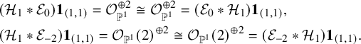 $$ \begin{align*} & (\mathcal{H}_1 \ast \mathcal{E}_{0}) \boldsymbol{1}_{(1,1)} = \mathcal{O}_{\mathbb{P}^1}^{\oplus 2} \cong \mathcal{O}_{\mathbb{P}^1}^{\oplus 2} = (\mathcal{E}_{0} \ast \mathcal{H}_{1}) \boldsymbol{1}_{(1,1)}, \\ &(\mathcal{H}_1 \ast \mathcal{E}_{-2}) \boldsymbol{1}_{(1,1)} = \mathcal{O}_{\mathbb{P}^1}(2)^{\oplus 2} \cong \mathcal{O}_{\mathbb{P}^1}(2)^{\oplus 2} = (\mathcal{E}_{-2} \ast \mathcal{H}_{1}) \boldsymbol{1}_{(1,1)}. \end{align*} $$
On the other hand, for
 $r=-1$
, we have the following exact triangle
$r=-1$
, we have the following exact triangle
 $$ \begin{align*} (\mathcal{H}_1 \ast \mathcal{E}_{-1}) \boldsymbol{1}_{(1,1)} = \mathcal{O}_{\mathbb{P}^1}(1)^{\oplus 2} \rightarrow (\mathcal{E}_{-1} \ast \mathcal{H}_1) \boldsymbol{1}_{(1,1)}= \mathcal{O}_{\mathbb{P}^1}(2) \oplus \mathcal{O}_{\mathbb{P}^1} \rightarrow \mathcal{O}_{\mathbb{P}^1}[1] \oplus \mathcal{O}_{\mathbb{P}^1} =\mathcal{E}_{0}\boldsymbol{1}_{(1,1)} \oplus \mathcal{E}_{0}\boldsymbol{1}_{(1,1)}[1]. \end{align*} $$
Remark 6.7. Like Proposition 6.4 and Proposition 6.6, similar results also hold for the convolutions of
 $\mathcal {H}_{-1}\boldsymbol {1}_{(1,1)}$
, which is given by
$\mathcal {H}_{-1}\boldsymbol {1}_{(1,1)}$
, which is given by
 $$ \begin{align*} \mathcal{H}_{-1}\boldsymbol{1}_{(1,1)} =\mathcal{O}_{2\Delta} \otimes \pi^*_1\mathcal{V}^{\otimes (-2)} \otimes \pi^*_2\mathcal{V}". \end{align*} $$
Finally, based on the above observation, we formulate a conjecture, which is the
 $\mathfrak {sl}_n$
version of Proposition 6.6.
$\mathfrak {sl}_n$
version of Proposition 6.6.
Conjecture 6.8.
-
1. We have the following exact triangles in
$\mathrm {D}^b(\mathrm {Fl}_{\underline {k}}(\mathbb {C}^N) \times \mathrm {Fl}_{\underline {k}+\alpha _i}(\mathbb {C}^N))$
and
$$ \begin{align*} &({\mathcal{H}}_{i,1} \ast {\mathcal{E}}_{i,-k_i})\boldsymbol{1}_{\underline{k}} \rightarrow ({\mathcal{E}}_{i,-k_i} \ast {\mathcal{H}}_{i,1})\boldsymbol{1}_{\underline{k}} \rightarrow ({\mathcal{E}}_{i,-k_i+1}\bigoplus {\mathcal{E}}_{i,-k_i+1}[1])\boldsymbol{1}_{\underline{k}}, \\ &({\mathcal{E}}_{i,-k_i}\ast {\mathcal{H}}_{i,-1})\boldsymbol{1}_{\underline{k}} \rightarrow ({\mathcal{H}}_{i,-1} \ast {\mathcal{E}}_{i,-k_i})\boldsymbol{1}_{\underline{k}} \rightarrow ({\mathcal{E}}_{i,-k_i-1}\bigoplus {\mathcal{E}}_{i,-k_i-1}[1])\boldsymbol{1}_{\underline{k}}, \end{align*} $$
for
$$ \begin{align*} ({\mathcal{H}}_{i,\pm 1} \ast {\mathcal{E}}_{i,r})\boldsymbol{1}_{\underline{k}} \cong ({\mathcal{E}}_{i,r} \ast {\mathcal{H}}_{i,\pm 1})\boldsymbol{1}_{\underline{k}} \end{align*} $$
$-k_i-1 \leq r \leq 0$
with
$r \neq -k_i$
.
-
2. We have the following exact triangles in
$\mathrm {D}^b(\mathrm {Fl}_{\underline {k}}(\mathbb {C}^N) \times \mathrm {Fl}_{\underline {k}-\alpha _i}(\mathbb {C}^N))$
and
$$ \begin{align*} &({\mathcal{F}}_{i,k_{i+1}} \ast {\mathcal{H}}_{i,1})\boldsymbol{1}_{\underline{k}} \rightarrow ({\mathcal{H}}_{i,1} \ast {\mathcal{F}}_{i,k_{i+1}})\boldsymbol{1}_{\underline{k}} \rightarrow ({\mathcal{F}}_{i,k_{i+1}+1}\bigoplus {\mathcal{F}}_{i,k_{i+1}+1}[1])\boldsymbol{1}_{\underline{k}}, \\ &({\mathcal{H}}_{i,-1} \ast {\mathcal{F}}_{i,k_{i+1}})\boldsymbol{1}_{\underline{k}} \rightarrow ({\mathcal{F}}_{i,k_{i+1}} \ast {\mathcal{H}}_{i,-1})\boldsymbol{1}_{\underline{k}} \rightarrow ({\mathcal{F}}_{i,k_{i+1}-1}\bigoplus {\mathcal{F}}_{i,k_{i+1}-1}[1])\boldsymbol{1}_{\underline{k}}, \end{align*} $$
for
$$ \begin{align*} ({\mathcal{H}}_{i,\pm 1} \ast {\mathcal{F}}_{i,s})\boldsymbol{1}_{\underline{k}} \cong ({\mathcal{F}}_{i,s}\ast {\mathcal{H}}_{i,\pm 1})\boldsymbol{1}_{\underline{k}} \end{align*} $$
$0 \leq s \leq k_{i+1}+1$
with
$s \neq k_{i+1}$
.


6.4 The Commutator Relation on the Grothendieck Groups for All Loop Generators
From Corollary 5.14, we know that there is an action of
 $\mathcal {U}$
on
$\mathcal {U}$
on
 $\bigoplus _{\underline {k}}K(\mathrm {Fl}_{\underline {k}}(\mathbb {C}^N))$
which comes from decategorifying the categorical
$\bigoplus _{\underline {k}}K(\mathrm {Fl}_{\underline {k}}(\mathbb {C}^N))$
which comes from decategorifying the categorical
 $\mathcal {U}$
-action in Theorem 5.6. Since the 1-morphisms act by FM transforms with kernels in Definition 5.5, the generators of
$\mathcal {U}$
-action in Theorem 5.6. Since the 1-morphisms act by FM transforms with kernels in Definition 5.5, the generators of
 $\mathcal {U}$
act on
$\mathcal {U}$
act on
 $\bigoplus _{\underline {k}}K(\mathrm {Fl}_{\underline {k}}(\mathbb {C}^N))$
by the K-theoretic FM transform. More precisely,
$\bigoplus _{\underline {k}}K(\mathrm {Fl}_{\underline {k}}(\mathbb {C}^N))$
by the K-theoretic FM transform. More precisely,
 $$ \begin{align*} e_{i,r}1_{\underline{k}}:K(\mathrm{Fl}_{\underline{k}}(\mathbb{C}^N)) \rightarrow K(\mathrm{Fl}_{\underline{k}+\alpha_{i}}(\mathbb{C}^N)), \ x \mapsto \pi_{2*}(\pi^{*}_{1}(x) \otimes [\iota(\underline{k})_{*}(\mathcal{V}_{i}/\mathcal{V}^{\prime}_{i})^{\otimes r}]) \end{align*} $$
where we denote
 $[\iota (\underline {k})_{*}(\mathcal {V}_{i}/\mathcal {V}^{\prime }_{i})^{\otimes r}]$
to be the class of
$[\iota (\underline {k})_{*}(\mathcal {V}_{i}/\mathcal {V}^{\prime }_{i})^{\otimes r}]$
to be the class of
 $\iota (\underline {k})_{*}(\mathcal {V}_{i}/\mathcal {V}^{\prime }_{i})^{\otimes r}$
in
$\iota (\underline {k})_{*}(\mathcal {V}_{i}/\mathcal {V}^{\prime }_{i})^{\otimes r}$
in
 $K(\mathrm {Fl}_{\underline {k}}(\mathbb {C}^N) \times \mathrm {Fl}_{\underline {k}+\alpha _{i}}(\mathbb {C}^N))$
, and similarly for
$K(\mathrm {Fl}_{\underline {k}}(\mathbb {C}^N) \times \mathrm {Fl}_{\underline {k}+\alpha _{i}}(\mathbb {C}^N))$
, and similarly for
 $f_{i,s}1_{\underline {k}}$
in the opposite direction. For other generators, it is direct to see that
$f_{i,s}1_{\underline {k}}$
in the opposite direction. For other generators, it is direct to see that
 $$ \begin{align*} &\psi_i^{+}1_{\underline{k}}:K(\mathrm{Fl}_{\underline{k}}(\mathbb{C}^N)) \rightarrow K(\mathrm{Fl}_{\underline{k}}(\mathbb{C}^N)), \ x \mapsto x \otimes (-1)^{k_{i+1}-1}[\det(\mathcal{V}_{i+1}/\mathcal{V}_i)] , \\ &\psi_i^{-}1_{\underline{k}}:K(\mathrm{Fl}_{\underline{k}}(\mathbb{C}^N)) \rightarrow K(\mathrm{Fl}_{\underline{k}}(\mathbb{C}^N)), \ x \mapsto x \otimes (-1)^{k_i-1}[\det(\mathcal{V}_i/\mathcal{V}_{i-1})^{-1}]. \end{align*} $$
As we mentioned at the beginning of this section, the FM kernels
 $\mathcal {E}_{i,r}\boldsymbol {1}_{\underline {k}}$
,
$\mathcal {E}_{i,r}\boldsymbol {1}_{\underline {k}}$
,
 $\mathcal {F}_{i,r}\boldsymbol {1}_{\underline {k}}$
are defined for all
$\mathcal {F}_{i,r}\boldsymbol {1}_{\underline {k}}$
are defined for all
 $r \in \mathbb {Z}$
. Thus, the action of
$r \in \mathbb {Z}$
. Thus, the action of
 $e_{i,r}1_{\underline {k}}$
,
$e_{i,r}1_{\underline {k}}$
,
 $f_{i,r}1_{\underline {k}}$
by K-theoretic FM transforms are also defined for all
$f_{i,r}1_{\underline {k}}$
by K-theoretic FM transforms are also defined for all
 $r \in \mathbb {Z}$
. In this subsection, we want to understand the commutator relation
$r \in \mathbb {Z}$
. In this subsection, we want to understand the commutator relation
 $[e_{i,r},f_{i,s}]1_{\underline {k}}$
for all
$[e_{i,r},f_{i,s}]1_{\underline {k}}$
for all
 $r,s \in \mathbb {Z}$
.
$r,s \in \mathbb {Z}$
.
It suffices to consider the
 $\mathfrak {sl}_2$
case where the action is on
$\mathfrak {sl}_2$
case where the action is on
 $\bigoplus _k K(\mathrm {Gr}(k,N))$
. Then, condition (10) gives the following commutator relation
$\bigoplus _k K(\mathrm {Gr}(k,N))$
. Then, condition (10) gives the following commutator relation
 $$ \begin{align} [e_{0},f_{N-k}]1_{(k,N-k)}&=\psi^+1_{(k,N-k)}=\otimes (-1)^{N-k-1}[\det(\mathbb{C}^N/\mathcal{V})], \nonumber \\ [e_{r},f_{s}]1_{(k,N-k)}&=0, \ \text{if} \ -k+1 \leq r+s \leq N-k-1, \\ \nonumber [e_{-k},f_{0}]1_{(k,N-k)}&=\psi^-1_{(k,N-k)}= \otimes (-1)^{k}[\det(\mathcal{V})^{-1}]. \end{align} $$
Moreover, the two exact triangles (6.2) and (6.3) give the following commutator relations
 $$ \begin{align} [e_{0},f_{N-k+1}]1_{(k,N-k)}&=\psi^+h_{1}1_{(k,N-k)}, \nonumber \\ [e_{-k-1},f_{0}]1_{(k,N-k)}&=-\psi^-h_{-1}1_{(k,N-k)}. \end{align} $$
To know the action of
 $h_{\pm 1}1_{(k,N-k)}$
, although their FM kernels
$h_{\pm 1}1_{(k,N-k)}$
, although their FM kernels
 $\mathcal {H}_{\pm 1}\boldsymbol {1}_{(k,N-k)}$
are complicate from (6.7) and (6.8), from Subsection 6.2 we know that
$\mathcal {H}_{\pm 1}\boldsymbol {1}_{(k,N-k)}$
are complicate from (6.7) and (6.8), from Subsection 6.2 we know that
 $\mathcal {H}_{1}\boldsymbol {1}_{(k,N-k)}$
fits in the exact triangle (6.16).
$\mathcal {H}_{1}\boldsymbol {1}_{(k,N-k)}$
fits in the exact triangle (6.16).
Passing to the Grothendieck group, we have the following equality in
 $K(\mathrm {Gr}(k,N) \times \mathrm {Gr}(k,N))$
 $$ \begin{align*} [\mathcal{H}_{1}\boldsymbol{1}_{(k,N-k)}]=[\Delta_{*}\mathcal{V}]+[\Delta_{*}\mathbb{C}^N/\mathcal{V}]=[\Delta_{*}\mathbb{C}^N]. \end{align*} $$
Thus the action of
 $h_{1}1_{(k,N-k)}$
is given by
$h_{1}1_{(k,N-k)}$
is given by
 $$ \begin{align*} h_{1}1_{(k,N-k)}:K(\mathrm{Gr}(k,N)) \rightarrow K(\mathrm{Gr}(k,N)), \ x \mapsto x \otimes [\mathbb{C}^N]. \end{align*} $$
A similar argument also shows that the action of
 $h_{-1}1_{(k,N-k)}$
is given by
$h_{-1}1_{(k,N-k)}$
is given by
 $$ \begin{align*} h_{-1}1_{(k,N-k)}:K(\mathrm{Gr}(k,N)) \rightarrow K(\mathrm{Gr}(k,N)), \ x \mapsto x \otimes [(\mathbb{C}^N)^{\vee}]. \end{align*} $$
Note that even though the convolutions between
 $\mathcal {H}_{1}\boldsymbol {1}_{(k,N-k)}$
and
$\mathcal {H}_{1}\boldsymbol {1}_{(k,N-k)}$
and
 $\Psi ^{+}\boldsymbol {1}_{(k,N-k)}$
are non-isomorphic in general when we pass to the Grothendieck group, they are commutative, i.e.,
$\Psi ^{+}\boldsymbol {1}_{(k,N-k)}$
are non-isomorphic in general when we pass to the Grothendieck group, they are commutative, i.e.,
 $\psi ^{+}h_{1}1_{(k,N-k)}=h_{1}\psi ^+1_{(k,N-k)}$
(similarly for
$\psi ^{+}h_{1}1_{(k,N-k)}=h_{1}\psi ^+1_{(k,N-k)}$
(similarly for
 $h_{-1}1_{(k,N-k)}$
and
$h_{-1}1_{(k,N-k)}$
and
 $\psi ^{-}1_{(k,N-k)}$
).
$\psi ^{-}1_{(k,N-k)}$
).
Next, it is standard to check that we have the following conjugation property
 $$ \begin{align*} e_r1_{(k,N-k)}&=(-1)^r(\psi^+)^re_0(\psi^+)^{-r}1_{(k,N-k)}=(-1)^r(\psi^-)^re_0(\psi^-)^{-r}1_{(k,N-k)}, \\ f_r1_{(k,N-k)}&=(-1)^r(\psi^+)^rf_0(\psi^+)^{-r}1_{(k,N-k)}=(-1)^r(\psi^-)^rf_0(\psi^-)^{-r}1_{(k,N-k)}, \end{align*} $$
for all
 $r \in \mathbb {Z}$
(see (3.2), (3.3), and (3.4) for their categorical version).
$r \in \mathbb {Z}$
(see (3.2), (3.3), and (3.4) for their categorical version).
The above conjugation property can help us to know other commutator relations. For example, we can write
 $$ \begin{align*} [e_{r},f_{s}]1_{(k,N-k)}&=e_rf_s1_{(k,N-k)}-f_se_r1_{(k,N-k)}=(\psi^{+})^re_0f_{r+s}(\psi^{+})^{-r}-(\psi^+)^rf_{r+s}e_0(\psi^+)^{-r}1_{(k,N-k)} \\ &=(\psi^+)^r[e_0,f_{r+s}](\psi^+)^{-r}1_{(k,N-k)}. \end{align*} $$
Thus, by applying suitable conjugation to (6.26) and (6.27), we obtain
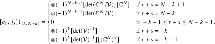 $$ \begin{align*} [e_{r},f_{s}]1_{(k,N-k)}= \begin{cases} \otimes (-1)^{N-k-1}[\det(\mathbb{C}^N/\mathcal{V})][\mathbb{C}^N] & \text{if} \ r+s=N-k+1 \\ \otimes (-1)^{N-k-1}[\det(\mathbb{C}^N/\mathcal{V})] & \text{if} \ r+s=N-k \\ 0 & \text{if} \ -k+1 \leq r+s \leq N-k-1 \\ \otimes (-1)^{k}[\det(\mathcal{V})^{-1}] & \text{if} \ r+s=-k \\ \otimes (-1)^{k}[\det(\mathcal{V})^{-1}][(\mathbb{C}^N)^{\vee}]& \text{if} \ r+s=-k-1 \end{cases}. \end{align*} $$
For the rest of the cases, we have to understand the categorical commutator relation between
 $\mathsf {E}_{r}\mathsf {F}_{s}\boldsymbol {1}_{(k,N-k)}$
and
$\mathsf {E}_{r}\mathsf {F}_{s}\boldsymbol {1}_{(k,N-k)}$
and
 $\mathsf {F}_{s}\mathsf {E}_{r}\boldsymbol {1}_{(k,N-k)}$
(or more precisely
$\mathsf {F}_{s}\mathsf {E}_{r}\boldsymbol {1}_{(k,N-k)}$
(or more precisely
 $(\mathcal {E}_{r} \ast \mathcal {F}_{s})\boldsymbol {1}_{(k,N-k)}$
and
$(\mathcal {E}_{r} \ast \mathcal {F}_{s})\boldsymbol {1}_{(k,N-k)}$
and
 $(\mathcal {F}_{s} \ast \mathcal {E}_{r})\boldsymbol {1}_{(k,N-k)}$
) for
$(\mathcal {F}_{s} \ast \mathcal {E}_{r})\boldsymbol {1}_{(k,N-k)}$
) for
 $r+s \geq N-k+2$
and
$r+s \geq N-k+2$
and
 $r+s \leq -k-2$
.
$r+s \leq -k-2$
.
Consider first case
 $r+s=N-k+2$
, similarly like Proposition 5.10, it suffices to compare
$r+s=N-k+2$
, similarly like Proposition 5.10, it suffices to compare
 $(\mathcal {E}_{0} \ast \mathcal {F}_{s})\boldsymbol {1}_{(k,N-k)}$
and
$(\mathcal {E}_{0} \ast \mathcal {F}_{s})\boldsymbol {1}_{(k,N-k)}$
and
 $(\mathcal {F}_{s} \ast \mathcal {E}_{0})\boldsymbol {1}_{(k,N-k)}$
for
$(\mathcal {F}_{s} \ast \mathcal {E}_{0})\boldsymbol {1}_{(k,N-k)}$
for
 $s=N-k+2$
.
$s=N-k+2$
.
Then like the exact triangle (6.1) we have the following exact triangle
 $$ \begin{align} p_{*} (\mathcal{V}"/\mathcal{V}"')^{\otimes (N-k+2)} \rightarrow p_{*}(\mathcal{V}'/\mathcal{V})^{\otimes (N-k+2)} \rightarrow p_{*}(\mathcal{O}_{(N-k+2)D} \otimes (\mathcal{V}'/\mathcal{V})^{\otimes (N-k+2)}) \end{align} $$
by applying
 $p_{*}$
to (5.16) with
$p_{*}$
to (5.16) with
 $n= N-k+2$
. Again, a similar argument as in the proof of Proposition 5.10 tells us that
$n= N-k+2$
. Again, a similar argument as in the proof of Proposition 5.10 tells us that
 $$ \begin{align*} p_{*}(\mathcal{O}_{(N-k+2)D} \otimes (\mathcal{V}'/\mathcal{V})^{\otimes (N-k+2)}) \cong p_{*}(\mathcal{O}_{(N-k+1)D} \otimes (\mathcal{V}'/\mathcal{V})^{\otimes (N-k+2)}) \cong ... \cong p_{*}(\mathcal{O}_{3D} \otimes (\mathcal{V}'/\mathcal{V})^{\otimes (N-k+2)}), \end{align*} $$
and applying
 $t_{*}$
to (6.28) we obtain the following exact triangle
$t_{*}$
to (6.28) we obtain the following exact triangle
 $$ \begin{align} (\mathcal{F}_{N-k+2} \ast \mathcal{E}_{0})\boldsymbol{1}_{(k,N-k)} \rightarrow (\mathcal{E}_{0} \ast \mathcal{F}_{N-k+2})\boldsymbol{1}_{(k,N-k)} \rightarrow t_{*}p_{*}(\mathcal{O}_{3D} \otimes (\mathcal{V}'/\mathcal{V})^{\otimes (N-k+2)}). \end{align} $$
Thus the first question is we have to study
 $t_{*}p_{*}(\mathcal {O}_{3D} \otimes (\mathcal {V}'/\mathcal {V})^{\otimes (N-k+2)})$
. Tensoring (5.17) with
$t_{*}p_{*}(\mathcal {O}_{3D} \otimes (\mathcal {V}'/\mathcal {V})^{\otimes (N-k+2)})$
. Tensoring (5.17) with
 $n=3$
by
$n=3$
by
 $(\mathcal {V}'/\mathcal {V})^{\otimes (N-k-1)}$
, we obtain
$(\mathcal {V}'/\mathcal {V})^{\otimes (N-k-1)}$
, we obtain
 $$ \begin{align*} \mathcal{O}_{D} \otimes (\mathcal{V}'/\mathcal{V})^{\otimes (N-k)} \otimes (\mathcal{V}/\mathcal{V}"')^{2} \rightarrow \mathcal{O}_{3D}\otimes (\mathcal{V}'/\mathcal{V})^{\otimes (N-k+2)} \rightarrow \mathcal{O}_{2D} \otimes (\mathcal{V}'/\mathcal{V})^{\otimes (N-k+2)} \end{align*} $$
applying
 $t_{*}p_{*}$
, using the projection formula and Proposition 4.4, we get the following exact triangle
$t_{*}p_{*}$
, using the projection formula and Proposition 4.4, we get the following exact triangle
 $$ \begin{align} \Delta_{*}\mathrm{Sym}^{2}(\mathcal{V}) \otimes \det(\mathbb{C}^N/\mathcal{V})[1+k-N]\rightarrow t_{*}p_{*}(\mathcal{O}_{3D}\otimes(\mathcal{V}'/\mathcal{V})^{\otimes N-k+2}) \rightarrow t_{*}p_{*}(\mathcal{O}_{2D}\otimes(\mathcal{V}'/\mathcal{V})^{\otimes N-k+2}). \end{align} $$
Next, tensoring (5.17) with
 $n=2$
by
$n=2$
by
 $(\mathcal {V}'/\mathcal {V})^{\otimes (N-k)}$
, we obtain
$(\mathcal {V}'/\mathcal {V})^{\otimes (N-k)}$
, we obtain
 $$ \begin{align*} \mathcal{O}_{D} \otimes (\mathcal{V}'/\mathcal{V})^{\otimes (N-k+1)} \otimes (\mathcal{V}/\mathcal{V}"') \rightarrow \mathcal{O}_{2D}\otimes (\mathcal{V}'/\mathcal{V})^{\otimes (N-k+2)} \rightarrow \mathcal{O}_{D}\otimes (\mathcal{V}'/\mathcal{V})^{\otimes (N-k+2)} \end{align*} $$
again applying
 $t_{*}p_{*}$
, using the projection formula and Proposition 4.4, we get the following exact triangle
$t_{*}p_{*}$
, using the projection formula and Proposition 4.4, we get the following exact triangle
 $$ \begin{align} \begin{split} &\Delta_{*}\mathcal{V} \otimes \mathbb{C}^N/\mathcal{V} \otimes \det(\mathbb{C}^N/\mathcal{V})[1+k-N]\rightarrow t_{*}p_{*}(\mathcal{O}_{2D}\otimes(\mathcal{V}'/\mathcal{V})^{\otimes (N-k+2)}) \\& \quad \rightarrow \Delta_{*}\mathrm{Sym}^{2}(\mathbb{C}^N/\mathcal{V}) \otimes \det(\mathbb{C}^N/\mathcal{V})[1+k-N]. \end{split} \end{align} $$
Thus, understanding
 $t_{*}p_{*}(\mathcal {O}_{3D} \otimes (\mathcal {V}'/\mathcal {V})^{\otimes (N-k+2)})$
is equivalent to understanding the two exact triangles (6.30) and (6.31). Moreover, we define
$t_{*}p_{*}(\mathcal {O}_{3D} \otimes (\mathcal {V}'/\mathcal {V})^{\otimes (N-k+2)})$
is equivalent to understanding the two exact triangles (6.30) and (6.31). Moreover, we define
 $$ \begin{align} \mathcal{H}_{2}\boldsymbol{1}_{(k,N-k)}&:=(\Psi^{+}\boldsymbol{1}_{(k,N-k)})^{-1} \ast [t_{*}p_{*}(\mathcal{O}_{3D} \otimes (\mathcal{V}'/\mathcal{V})^{\otimes (N-k+2)})] \nonumber \\ &=t_{*}p_{*}(\mathcal{O}_{3D} \otimes (\mathcal{V}'/\mathcal{V})^{\otimes (N-k+2)}) \otimes \pi^*_{2}\det(\mathbb{C}^N/\mathcal{V})^{-1}[N-k-1] \in \mathrm{D}^b(\mathrm{Gr}(k,N)\times \mathrm{Gr}(k,N)) \end{align} $$
which can be thought of as an FM kernel for a certain (undefined) 1-morphism
 $\mathsf {{H}}_{2}\boldsymbol {1}_{(k,N-k)}$
. Then
$\mathsf {{H}}_{2}\boldsymbol {1}_{(k,N-k)}$
. Then
 $\mathcal {H}_{2}\boldsymbol {1}_{(k,N-k)}$
is build up from the following two exact triangles in
$\mathcal {H}_{2}\boldsymbol {1}_{(k,N-k)}$
is build up from the following two exact triangles in
 $\mathrm {D}^b(\mathrm {Gr}(k,N) \times \mathrm {Gr}(k,N))$
 $$ \begin{align} &\Delta_{*}\mathrm{Sym}^{2}(\mathcal{V}) \rightarrow \mathcal{H}_{2}\boldsymbol{1}_{(k,N-k)} \rightarrow (\Psi^{+}\boldsymbol{1}_{(k,N-k)})^{-1} \ast [t_{*}p_{*}(\mathcal{O}_{2D}\otimes(\mathcal{V}'/\mathcal{V})^{\otimes (N-k+2)})], \end{align} $$
 $$ \begin{align} &\Delta_{*}\mathcal{V} \otimes \mathbb{C}^N/\mathcal{V} \rightarrow (\Psi^{+}\boldsymbol{1}_{(k,N-k)})^{-1} \ast [t_{*}p_{*}(\mathcal{O}_{2D}\otimes(\mathcal{V}'/\mathcal{V})^{\otimes (N-k+2)})] \rightarrow \Delta_{*}\mathrm{Sym}^{2}(\mathbb{C}^N/\mathcal{V}). \end{align} $$
Remark 6.9. Another natural question to ask is what is the categorical commutator relation between
 $\mathsf {{H}}_{2}\mathsf {E}_{r}\boldsymbol {1}_{(k,N-k)}$
and
$\mathsf {{H}}_{2}\mathsf {E}_{r}\boldsymbol {1}_{(k,N-k)}$
and
 $\mathsf {E}_{r}\mathsf {{H}}_{2}\boldsymbol {1}_{(k,N-k)}$
(or exact triangle relates
$\mathsf {E}_{r}\mathsf {{H}}_{2}\boldsymbol {1}_{(k,N-k)}$
(or exact triangle relates
 $\mathcal {H}_{2} \ast {\mathcal {E}}_{r}\boldsymbol {1}_{(k,N-k)}$
and
$\mathcal {H}_{2} \ast {\mathcal {E}}_{r}\boldsymbol {1}_{(k,N-k)}$
and
 ${\mathcal {E}}_{r} \ast \mathcal {H}_{2}\boldsymbol {1}_{(k,N-k)}$
). Due to the difficulty and complication, we will like to address those questions in the future and similar for other comparisons between
${\mathcal {E}}_{r} \ast \mathcal {H}_{2}\boldsymbol {1}_{(k,N-k)}$
). Due to the difficulty and complication, we will like to address those questions in the future and similar for other comparisons between
 $\mathsf {{H}}_{n}\mathsf {E}_{r}\boldsymbol {1}_{(k,N-k)}$
and
$\mathsf {{H}}_{n}\mathsf {E}_{r}\boldsymbol {1}_{(k,N-k)}$
and
 $\mathsf {E}_{r}\mathsf {{H}}_{n}\boldsymbol {1}_{(k,N-k)}$
with
$\mathsf {E}_{r}\mathsf {{H}}_{n}\boldsymbol {1}_{(k,N-k)}$
with
 $n \geq 3$
.
$n \geq 3$
.
However, the above discussions can help us to understand what exactly are the commutators for the loop generators
 $e_{r}1_{(k,N-k)}$
,
$e_{r}1_{(k,N-k)}$
,
 $f_{s}1_{(k,N-k)}$
at the level of Grothendieck groups. From (6.33) and (6.34), we have the following equality in
$f_{s}1_{(k,N-k)}$
at the level of Grothendieck groups. From (6.33) and (6.34), we have the following equality in
 $K(\mathrm {Gr}(k,N) \times \mathrm {Gr}(k,N))$
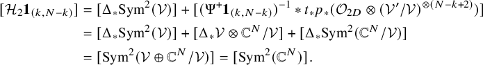 $$ \begin{align*} [\mathcal{H}_{2}\boldsymbol{1}_{(k,N-k)}] &= [\Delta_{*}\mathrm{Sym}^{2}(\mathcal{V})] + [(\Psi^{+}\boldsymbol{1}_{(k,N-k)})^{-1} \ast t_{*}p_{*}(\mathcal{O}_{2D}\otimes(\mathcal{V}'/\mathcal{V})^{\otimes (N-k+2)}) ] \\ &=[\Delta_{*}\mathrm{Sym}^{2}(\mathcal{V})] + [\Delta_{*}\mathcal{V} \otimes \mathbb{C}^N/\mathcal{V}] +[\Delta_{*}\mathrm{Sym}^{2}(\mathbb{C}^N/\mathcal{V})] \\ & = [\mathrm{Sym}^2(\mathcal{V} \oplus \mathbb{C}^N/\mathcal{V})]=[\mathrm{Sym}^{2}(\mathbb{C}^N)]. \end{align*} $$
Thus, by the definition of
 $\mathcal {H}_{2}\boldsymbol {1}_{(k,N-k)}$
and the exact triangle (6.29), we get the following commutator relation after a suitable conjugation
$\mathcal {H}_{2}\boldsymbol {1}_{(k,N-k)}$
and the exact triangle (6.29), we get the following commutator relation after a suitable conjugation
 $$ \begin{align*} [e_{r},f_{s}]1_{(k,N-k)}=\otimes (-1)^{N-k-1} [\mathrm{Sym}^2(\mathbb{C}^N)][\det(\mathbb{C}^N/\mathcal{V})], \ \text{if} \ r+s=N-k+2. \end{align*} $$
The above argument can be applied to other cases where
 $r+s \geq N-k+3$
and similarly
$r+s \geq N-k+3$
and similarly
 $r+s \leq -k-2$
. Moreover, the result can be generalized to the
$r+s \leq -k-2$
. Moreover, the result can be generalized to the
 $\mathfrak {sl}_n$
case directly. In conclusion, we have the following result.
$\mathfrak {sl}_n$
case directly. In conclusion, we have the following result.
Corollary 6.10. The commutator relations at the level of Grothendieck groups
 $K(\mathrm {Fl}_{\underline {k}}(\mathbb {C}^N))$
for all
$K(\mathrm {Fl}_{\underline {k}}(\mathbb {C}^N))$
for all
 $e_{i,r}1_{\underline {k}}$
,
$e_{i,r}1_{\underline {k}}$
,
 $f_{i,s}1_{\underline {k}}$
with
$f_{i,s}1_{\underline {k}}$
with
 $r,s \in \mathbb {Z}$
is given by
$r,s \in \mathbb {Z}$
is given by
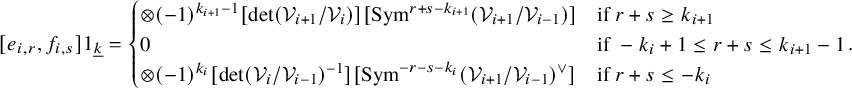 $$ \begin{align*} [e_{i,r},f_{i,s}]1_{\underline{k}}= \begin{cases} \otimes (-1)^{k_{i+1}-1}[\det(\mathcal{V}_{i+1}/\mathcal{V}_{i})][\mathrm{Sym}^{r+s-k_{i+1}}(\mathcal{V}_{i+1}/\mathcal{V}_{i-1})] & \text{if} \ r+s \geq k_{i+1} \\ 0 & \text{if} \ -k_{i}+1 \leq r+s \leq k_{i+1}-1 \\ \otimes (-1)^{k_{i}}[\det(\mathcal{V}_{i}/\mathcal{V}_{i-1})^{-1}][\mathrm{Sym}^{-r-s-k_{i}}(\mathcal{V}_{i+1}/\mathcal{V}_{i-1})^{\vee}]& \text{if} \ r+s \leq -k_{i} \end{cases}. \end{align*} $$
Finally, we give a remark.
Remark 6.11. It would be interesting to find an integral basis for
 $K(\mathrm {Fl}_{\underline {k}}(\mathbb {C}^N))$
and compute the matrix elements of the generators
$K(\mathrm {Fl}_{\underline {k}}(\mathbb {C}^N))$
and compute the matrix elements of the generators
 $e_{i,r}1_{\underline {k}}$
and
$e_{i,r}1_{\underline {k}}$
and
 $f_{i,s}1_{\underline {k}}$
.
$f_{i,s}1_{\underline {k}}$
.
7 Categorical Action of the Affine 0-Hecke Algebras
In this final section, we apply the categorical action of the shifted 0-affine algebra, i.e., Theorem 5.6, to construct categorical action of the affine 0-Hecke algebra on the derived category of coherent sheaves on the full flag variety.
7.1 Affine 0-Hecke Algebras
We begin with the definition of the affine 0-Hecke algebras of type A.
Definition 7.1. The affine 0-Hecke algebra
 $\mathcal {H}_{N}(0)$
is defined to be the unital associative
$\mathcal {H}_{N}(0)$
is defined to be the unital associative
 $\mathbb {C}$
-algebra generated by the elements
$\mathbb {C}$
-algebra generated by the elements
 $T_{1},...,T_{N-1}$
and the polynomial algebra
$T_{1},...,T_{N-1}$
and the polynomial algebra
 $\mathbb {C}[X_{1}^{\pm 1},...,X_{N}^{\pm 1}]$
subject to the following relations
$\mathbb {C}[X_{1}^{\pm 1},...,X_{N}^{\pm 1}]$
subject to the following relations
 $$ \begin{align} T_{i}^2=T_{i}, \end{align} $$
 $$ \begin{align} T_{i}T_{i+1}T_{i}=T_{i+1}T_{i}T_{i+1}, \ T_{i}T_{j}=T_{j}T_{i}, \ \text{if} \ |i-j| \geq 2, \end{align} $$
 $$ \begin{align} T_{i}X_{j}=X_{j}T_{i} \ \text{if} \ j \neq i,i+1, \end{align} $$
 $$ \begin{align} X_{i+1}T_{i}=T_{i}X_{i}+X_{i+1}, \end{align} $$
 $$ \begin{align} X_{i}T_{i}=T_{i}X_{i+1}-X_{i+1}. \end{align} $$
We give a remark about the affine 0-Hecke algebra.
Remark 7.2. The affine 0-Hecke algebra is the affine Hecke algebra with variable q specialized at
 $0$
.
$0$
.
Next, we recall the action of
 $\mathcal {H}_{N}(0)$
on the Grothendieck group of the full flag variety. Let
$\mathcal {H}_{N}(0)$
on the Grothendieck group of the full flag variety. Let
 $G=\mathrm {SL}_{N}(\mathbb {C})$
and
$G=\mathrm {SL}_{N}(\mathbb {C})$
and
 $B \subset G$
be the Borel of upper triangular matrices. Then, the full flag variety is defined by
$B \subset G$
be the Borel of upper triangular matrices. Then, the full flag variety is defined by
 $$ \begin{align} G/B:=\{0 \subset V_{1} \subset V_{2} \subset ... \subset V_{N}=\mathbb{C}^N \ | \ \dim V_{k}=k \ \text{for} \ \text{all} \ k \}. \end{align} $$
The Weyl group W is isomorphic to the symmetric group, denoted by
 $S_N$
. Let
$S_N$
. Let
 $\{s_1,...,s_{N-1}\}$
be the simple reflections that generate the Weyl group
$\{s_1,...,s_{N-1}\}$
be the simple reflections that generate the Weyl group
 $W=S_{N}$
. Then, for each
$W=S_{N}$
. Then, for each
 $1 \leq i \leq N-1$
, there is the minimal parabolic subgroup
$1 \leq i \leq N-1$
, there is the minimal parabolic subgroup
 $P_i=B \cup Bs_iB$
. Similarly, the quotient
$P_i=B \cup Bs_iB$
. Similarly, the quotient
 $G/P_i$
, which is called a partial flag variety, can be identified with the following space
$G/P_i$
, which is called a partial flag variety, can be identified with the following space
 $$ \begin{align} G/P_{i}:=\{0 \subset V_{1} \subset V_{2} \subset ... \subset V_{i-1} \subset V_{i+1} \subset ... \subset V_{N}=\mathbb{C}^N \ | \ \dim V_{k} =k \ \text{for} \ k \neq i \}. \end{align} $$
There are natural projections
 $\pi _{i}:G/B \rightarrow G/P_{i}$
where
$\pi _{i}:G/B \rightarrow G/P_{i}$
where
 $ 1 \leq i \leq N-1$
, which obviously are
$ 1 \leq i \leq N-1$
, which obviously are
 $\mathbb {P}^1$
-fibrations. Those maps induce pushforwards
$\mathbb {P}^1$
-fibrations. Those maps induce pushforwards
 $\pi _{i_*}:K(G/B) \rightarrow K(G/P_{i})$
and pullbacks
$\pi _{i_*}:K(G/B) \rightarrow K(G/P_{i})$
and pullbacks
 $\pi _{i}^*:K(G/P_{i}) \rightarrow K(G/B)$
where
$\pi _{i}^*:K(G/P_{i}) \rightarrow K(G/B)$
where
 $1 \leq i \leq N-1$
. Then the fundamental construction of the push-pull operators gives the Demazure operators
$1 \leq i \leq N-1$
. Then the fundamental construction of the push-pull operators gives the Demazure operators
 $T_{i}:=\pi _{i}^*\pi _{i_*}:K(G/B) \rightarrow K(G/B)$
for all
$T_{i}:=\pi _{i}^*\pi _{i_*}:K(G/B) \rightarrow K(G/B)$
for all
 $1 \leq i \leq N-1$
.
$1 \leq i \leq N-1$
.
On
 $G/B$
, we denote
$G/B$
, we denote
 $\mathcal {V}_{i}$
to be the tautological bundle of rank i for all
$\mathcal {V}_{i}$
to be the tautological bundle of rank i for all
 $1 \leq i \leq N$
. Let
$1 \leq i \leq N$
. Let
 $a_{i}=[\mathcal {V}_{i}/\mathcal {V}_{i-1}]$
be the class of the tautological line bundle
$a_{i}=[\mathcal {V}_{i}/\mathcal {V}_{i-1}]$
be the class of the tautological line bundle
 $\mathcal {V}_{i}/\mathcal {V}_{i-1}$
in
$\mathcal {V}_{i}/\mathcal {V}_{i-1}$
in
 $K(G/B)$
, where
$K(G/B)$
, where
 $1 \leq i \leq N$
. Then,
$1 \leq i \leq N$
. Then,
 $K(G/B)$
admits a presentation, which is called the Borel presentation.
$K(G/B)$
admits a presentation, which is called the Borel presentation.
 $$ \begin{align} K(G/B) \cong \mathbb{C}[a_1^{\pm},...,a_N^{\pm}] {\bigg/} \left \langle e_i- {N \choose i} \right \rangle \end{align} $$
where
 $\langle e_i- {N\choose i} \rangle $
is the ideal generated by
$\langle e_i- {N\choose i} \rangle $
is the ideal generated by
 $\{e_i- {N\choose i}\}_{i=1}^{N}$
, and
$\{e_i- {N\choose i}\}_{i=1}^{N}$
, and
 $e_i$
is the i-th elementary symmetric polynomial in
$e_i$
is the i-th elementary symmetric polynomial in
 $a_1, a_2,...,a_{N}$
.
$a_1, a_2,...,a_{N}$
.
Under the presentation (7.3),
 $T_{i}$
has the following explicit description
$T_{i}$
has the following explicit description
 $$ \begin{align*} T_{i}=\frac{a_{i+1}-a_is_{i}}{a_{i+1}-a_i} \end{align*} $$
where
 $s_i$
is the simple reflection that permutes
$s_i$
is the simple reflection that permutes
 $a_i$
and
$a_i$
and
 $a_{i+1}$
for all
$a_{i+1}$
for all
 $ 1 \leq i \leq N-1$
. Finally, we define the operator
$ 1 \leq i \leq N-1$
. Finally, we define the operator
 $X_{j}:K(G/B) \rightarrow K(G/B)$
to be multiplication by
$X_{j}:K(G/B) \rightarrow K(G/B)$
to be multiplication by
 $a_{j}$
for all
$a_{j}$
for all
 $1 \leq j \leq N$
.
$1 \leq j \leq N$
.
Then it is easy to check that those operators
 $T_{i}$
,
$T_{i}$
,
 $X_{j}^{\pm 1}$
defined in such a way satisfy relations relations (H01) to (H05) in Definition 7.1. Thus we get an action of
$X_{j}^{\pm 1}$
defined in such a way satisfy relations relations (H01) to (H05) in Definition 7.1. Thus we get an action of
 $\mathcal {H}_{N}(0)$
on
$\mathcal {H}_{N}(0)$
on
 $K(G/B)$
.
$K(G/B)$
.
It is natural to lift this action to the categorical level. More precisely, we replace
 $K(G/B)$
by the derived category of coherent sheaves
$K(G/B)$
by the derived category of coherent sheaves
 $\mathrm {D}^b(G/B)$
and we need to define certain functors
$\mathrm {D}^b(G/B)$
and we need to define certain functors
 $\mathbb {T}_{i}:\mathrm {D}^b(G/B) \rightarrow \mathrm {D}^b(G/B)$
and
$\mathbb {T}_{i}:\mathrm {D}^b(G/B) \rightarrow \mathrm {D}^b(G/B)$
and
 $\mathbb {X}_{j}:\mathrm {D}^b(G/B) \rightarrow \mathrm {D}^b(G/B)$
that satisfy categorical version of the relations (H01) to (H05). Again, we would use the tools of FM transforms/kernels from Section 4 to define the categorical action.
$\mathbb {X}_{j}:\mathrm {D}^b(G/B) \rightarrow \mathrm {D}^b(G/B)$
that satisfy categorical version of the relations (H01) to (H05). Again, we would use the tools of FM transforms/kernels from Section 4 to define the categorical action.
We know that
 $T_{i}:=\pi _{i}^*\pi _{i_*}$
are defined by using the projection maps
$T_{i}:=\pi _{i}^*\pi _{i_*}$
are defined by using the projection maps
 $\pi _{i}:G/B \rightarrow G/P_{i}$
. Since
$\pi _{i}:G/B \rightarrow G/P_{i}$
. Since
 $\pi _{i}$
also induces functors on derived categories of coherent sheaves, i.e. the derived pushforward
$\pi _{i}$
also induces functors on derived categories of coherent sheaves, i.e. the derived pushforward
 $\pi _{i*}:\mathrm {D}^b(G/B) \rightarrow \mathrm {D}^b(G/P_{i})$
and the derived pullback
$\pi _{i*}:\mathrm {D}^b(G/B) \rightarrow \mathrm {D}^b(G/P_{i})$
and the derived pullback
 $\pi _{i}^{*}:\mathrm {D}^b(G/P_{i}) \rightarrow \mathrm {D}^b(G/B)$
, it is natural to define the functors
$\pi _{i}^{*}:\mathrm {D}^b(G/P_{i}) \rightarrow \mathrm {D}^b(G/B)$
, it is natural to define the functors
 $\mathbb {T}_{i}:=\pi _{i}^*\pi _{i_*}:\mathrm {D}^b(G/B) \rightarrow \mathrm {D}^b(G/B)$
for all
$\mathbb {T}_{i}:=\pi _{i}^*\pi _{i_*}:\mathrm {D}^b(G/B) \rightarrow \mathrm {D}^b(G/B)$
for all
 $1 \leq i \leq N-1$
.
$1 \leq i \leq N-1$
.
In fact,
 $\mathbb {T}_{i}$
are also FM transforms. Recall that for a morphism
$\mathbb {T}_{i}$
are also FM transforms. Recall that for a morphism
 $f:X \rightarrow Y$
between smooth projective varieties, the derived pushforward
$f:X \rightarrow Y$
between smooth projective varieties, the derived pushforward
 $f_{*}:\mathrm {D}^b(X) \rightarrow \mathrm {D}^b(Y)$
is isomorphic to the FM transform with kernel
$f_{*}:\mathrm {D}^b(X) \rightarrow \mathrm {D}^b(Y)$
is isomorphic to the FM transform with kernel
 $\mathcal {O}_{\Gamma _{f}}$
, where
$\mathcal {O}_{\Gamma _{f}}$
, where
 $\Gamma _{f}=(id \times f)(X)$
is the graph of f in
$\Gamma _{f}=(id \times f)(X)$
is the graph of f in
 $X \times Y$
. Similarly, the derived pullback
$X \times Y$
. Similarly, the derived pullback
 $f^*$
is isomorphic to the FM transform with kernel
$f^*$
is isomorphic to the FM transform with kernel
 $\mathcal {O}_{(f \times id)(X)}$
in
$\mathcal {O}_{(f \times id)(X)}$
in
 $\mathrm {D}^b(Y \times X)$
.
$\mathrm {D}^b(Y \times X)$
.
Thus, a simple calculation of the convolution of FM kernels shows that
 $$ \begin{align*} \mathbb{T}_{i} \cong \Phi_{\mathcal{O}_{(\pi_{i} \times id)(G/B)}} \circ \Phi_{\mathcal{O}_{(id \times \pi_i)(G/B)}} \cong \Phi_{\mathcal{T}_{i}} \end{align*} $$
where
 $\mathcal {T}_{i} \cong \mathcal {O}_{G/B \times _{G/P_{i}} G/B}$
for all
$\mathcal {T}_{i} \cong \mathcal {O}_{G/B \times _{G/P_{i}} G/B}$
for all
 $1 \leq i \leq N-1$
.
$1 \leq i \leq N-1$
.
The fibered product variety
 $G/B \times _{G/P_{i}} G/B$
is called the Bott-Samelson variety for
$G/B \times _{G/P_{i}} G/B$
is called the Bott-Samelson variety for
 $s_{i}$
. Thus, the FM transform with kernel given by structure sheaf of the Bott-Samelson variety for
$s_{i}$
. Thus, the FM transform with kernel given by structure sheaf of the Bott-Samelson variety for
 $s_{i}$
categorifies the Demazure operator
$s_{i}$
categorifies the Demazure operator
 $T_{i}$
for all
$T_{i}$
for all
 $1 \leq i \leq N-1$
.
$1 \leq i \leq N-1$
.
Next, we define the functors
 $\mathbb {X}_{j}$
. Since
$\mathbb {X}_{j}$
. Since
 $X_{j}$
is the map given by multiplication with the element
$X_{j}$
is the map given by multiplication with the element
 $a_{j}=[\mathcal {V}_{j}/\mathcal {V}_{j-1}]$
on the Grothendieck group, it is natural to define
$a_{j}=[\mathcal {V}_{j}/\mathcal {V}_{j-1}]$
on the Grothendieck group, it is natural to define
 $\mathbb {X}_{j}$
to be the functor that is given by tensoring the line bundle
$\mathbb {X}_{j}$
to be the functor that is given by tensoring the line bundle
 $\mathcal {V}_{j}/\mathcal {V}_{j-1}$
. Thus its FM kernel is given by
$\mathcal {V}_{j}/\mathcal {V}_{j-1}$
. Thus its FM kernel is given by
 $\mathcal {X}_{j}=\Delta _{*}(\mathcal {V}_{j}/\mathcal {V}_{j-1}) \in \mathrm {D}^b(G/B \times G/B)$
for all
$\mathcal {X}_{j}=\Delta _{*}(\mathcal {V}_{j}/\mathcal {V}_{j-1}) \in \mathrm {D}^b(G/B \times G/B)$
for all
 $1\leq j \leq N$
, where
$1\leq j \leq N$
, where
 $\Delta :G/B \rightarrow G/B \times G/B$
is the diagonal map. Since line bundles are invertible, we can define its inverse functor
$\Delta :G/B \rightarrow G/B \times G/B$
is the diagonal map. Since line bundles are invertible, we can define its inverse functor
 $\mathbb {X}_{j}^{-1}$
with FM kernel given by
$\mathbb {X}_{j}^{-1}$
with FM kernel given by
 $\mathcal {X}_{j}^{-1}=\Delta _{*}((\mathcal {V}_{j}/\mathcal {V}_{j-1})^{-1}) \in \mathrm {D}^b(G/B \times G/B)$
.
$\mathcal {X}_{j}^{-1}=\Delta _{*}((\mathcal {V}_{j}/\mathcal {V}_{j-1})^{-1}) \in \mathrm {D}^b(G/B \times G/B)$
.
With all the above settings, we can prove the following theorem, which says that there is a categorical action of the affine 0-Hecke algebra on
 $\mathrm {D}^b(G/B)$
. More precisely, we lift the relations (H01) to (H05) in Definition 7.1 to the categorical level, which are (7.4) to (7.8), respectively in Theorem 7.3. The proof will be given in the next subsection.
$\mathrm {D}^b(G/B)$
. More precisely, we lift the relations (H01) to (H05) in Definition 7.1 to the categorical level, which are (7.4) to (7.8), respectively in Theorem 7.3. The proof will be given in the next subsection.
Theorem 7.3. There is a categorical action of the affine 0-Hecke algebra
 $\mathcal {H}_{N}(0)$
on
$\mathcal {H}_{N}(0)$
on
 $\mathrm {D}^b(G/B)$
. More precisely, if we define the FM kernels
$\mathrm {D}^b(G/B)$
. More precisely, if we define the FM kernels
 $\mathcal {T}_{i}=\mathcal {O}_{G/B \times _{G/P_{i}} G/B}$
and
$\mathcal {T}_{i}=\mathcal {O}_{G/B \times _{G/P_{i}} G/B}$
and
 $\mathcal {X}_{j}=\Delta _{*}(\mathcal {V}_{j}/\mathcal {V}_{j-1})$
for
$\mathcal {X}_{j}=\Delta _{*}(\mathcal {V}_{j}/\mathcal {V}_{j-1})$
for
 $1 \leq i \leq N-1$
,
$1 \leq i \leq N-1$
,
 $1 \leq j \leq N$
, then we have the following categorical relations
$1 \leq j \leq N$
, then we have the following categorical relations
 $$ \begin{align} \mathcal{T}_{i} \ast \mathcal{T}_{i} \cong \mathcal{T}_{i}, \end{align} $$
 $$ \begin{align} \mathcal{T}_{i}\ast \mathcal{T}_{i+1} \ast \mathcal{T}_{i} \cong \mathcal{T}_{i+1} \ast \mathcal{T}_{i} \ast \mathcal{T}_{i+1}, \ \mathcal{T}_{i}\ast \mathcal{T}_{j} \cong \mathcal{T}_{j}\ast \mathcal{T}_{i} \ \text{if} \ |i-j| \geq 2, \end{align} $$
 $$ \begin{align} \mathcal{T}_{i}\ast \mathcal{X}_{j}\cong \mathcal{X}_{j} \ast \mathcal{T}_{i} \ \text{if} \ j \neq i,i+1, \end{align} $$
We have the following exact triangles in
 $\mathrm {D}^b(G/B \times G/B)$
 $$ \begin{align} \mathcal{T}_{i}\ast \mathcal{X}_{i} \rightarrow \mathcal{X}_{i+1}\ast \mathcal{T}_{i} \rightarrow \mathcal{X}_{i+1}, \end{align} $$
 $$ \begin{align} \mathcal{X}_{i} \ast \mathcal{T}_{i} \rightarrow \mathcal{T}_{i} \ast \mathcal{X}_{i+1} \rightarrow \mathcal{X}_{i+1}. \end{align} $$
7.2 Application by the Shifted 0-Affine Algebra
In this section, instead of proving Theorem 7.3 by direct computation of convolution of kernels, we use the theory of categorical action of the shifted 0-affine algebra, which was developed in Section 3 and Section 5 to help us prove the theorem.
To use the results of categorical action, i.e., Theorem 5.6 and Definition 3.1, the main idea is to interpret the Demazure operators in terms of elements in the shifted 0-affine algebra.
Recall that the Demazure operators are given by
 $T_{i}:=\pi ^{*}_{i}\pi _{i*}:K(G/B) \rightarrow K(G/B)$
where
$T_{i}:=\pi ^{*}_{i}\pi _{i*}:K(G/B) \rightarrow K(G/B)$
where
 $\pi _{i}:G/B \rightarrow G/P_{i}$
is the natural
$\pi _{i}:G/B \rightarrow G/P_{i}$
is the natural
 $\mathbb {P}^1$
-fibration with
$\mathbb {P}^1$
-fibration with
 $1 \leq i \leq N-1$
. With the notation of n-step partial flag variety (5.5), the full flag variety in (7.1) can be written as
$1 \leq i \leq N-1$
. With the notation of n-step partial flag variety (5.5), the full flag variety in (7.1) can be written as
 $G/B=\mathrm {Fl}_{(1,1,...,1)}(\mathbb {C}^N)$
. For the partial flag varieties in (7.2), we observe that
$G/B=\mathrm {Fl}_{(1,1,...,1)}(\mathbb {C}^N)$
. For the partial flag varieties in (7.2), we observe that
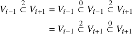 $$ \begin{align*} V_{i-1} \overset{2}{\subset} V_{i+1} & = V_{i-1} \overset{0}{\subset} V_{i-1} \overset{2}{\subset} V_{i+1} \\ & = V_{i-1} \overset{2}{\subset} V_{i+1} \overset{0}{\subset} V_{i+1} \end{align*} $$
where the number above the inclusions is the jump of dimensions. Thus they can be written as
 $G/P_{i}=\mathrm {Fl}_{(1,1,..,1)+\alpha _{i}}(\mathbb {C}^N)=\mathrm {Fl}_{(1,1,..,1)-\alpha _{i}}(\mathbb {C}^N)$
where
$G/P_{i}=\mathrm {Fl}_{(1,1,..,1)+\alpha _{i}}(\mathbb {C}^N)=\mathrm {Fl}_{(1,1,..,1)-\alpha _{i}}(\mathbb {C}^N)$
where
 $1 \leq i \leq N-1$
.
$1 \leq i \leq N-1$
.
We have the following diagram
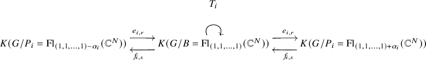
where
 $e_{i,r}1_{(1,1,...,1)}$
,
$e_{i,r}1_{(1,1,...,1)}$
,
 $e_{i,r}1_{(1,1,...,1)-\alpha _{i}}$
,
$e_{i,r}1_{(1,1,...,1)-\alpha _{i}}$
,
 $f_{i,s}1_{(1,1,...,1)}$
, and
$f_{i,s}1_{(1,1,...,1)}$
, and
 $f_{i,s}1_{(1,1,...,1)+\alpha _{i}}$
are elements in
$f_{i,s}1_{(1,1,...,1)+\alpha _{i}}$
are elements in
 $\dot {\mathrm {\mathbf {U}}}_{0,N}(L\mathfrak {sl}_{N})$
. Thus we can try to interpret
$\dot {\mathrm {\mathbf {U}}}_{0,N}(L\mathfrak {sl}_{N})$
. Thus we can try to interpret
 $T_{i}$
in terms of elements in
$T_{i}$
in terms of elements in
 $\dot {\mathrm {\mathbf {U}}}_{0,N}(L\mathfrak {sl}_{N})$
.
$\dot {\mathrm {\mathbf {U}}}_{0,N}(L\mathfrak {sl}_{N})$
.
Since we define both the action of
 $\dot {\mathrm {\mathbf {U}}}_{0,N}(L\mathfrak {sl}_{N})$
and the action of the Demazure operators
$\dot {\mathrm {\mathbf {U}}}_{0,N}(L\mathfrak {sl}_{N})$
and the action of the Demazure operators
 $T_{i}$
on derived categories by using FM transforms/kernels, to relate the 1-morphisms in the categorical
$T_{i}$
on derived categories by using FM transforms/kernels, to relate the 1-morphisms in the categorical
 $\dot {\mathrm {\mathbf {U}}}_{0,N}(L\mathfrak {sl}_{N})$
-action to
$\dot {\mathrm {\mathbf {U}}}_{0,N}(L\mathfrak {sl}_{N})$
-action to
 $\mathbb {T}_{i}$
, we have to compare their kernels.
$\mathbb {T}_{i}$
, we have to compare their kernels.
By definition, we have
 $\mathcal {E}_{i,0}1_{(1,1,..,1)}=\iota _{*}\mathcal {O}_{W^{1}_{i}((1,1,...,1))}$
, where
$\mathcal {E}_{i,0}1_{(1,1,..,1)}=\iota _{*}\mathcal {O}_{W^{1}_{i}((1,1,...,1))}$
, where
 $$ \begin{align*} W^{1}_{i}((1,1,...,1)):=\{(V_{\bullet},V_{\bullet}') \in \mathrm{Fl}_{(1,1,..,1)}(\mathbb{C}^N) \times \mathrm{Fl}_{(1,1,..,1)+\alpha_{i}}(\mathbb{C}^N) \ | \ V_{j}=V^{\prime}_{j} \ \mathrm{for} \ j \neq i, \ \mathrm{and} \ V^{\prime}_{i} \subset V_{i}\} \end{align*} $$
and
 $\iota :W^{1}_{i}((1,1,...,1)) \rightarrow \mathrm {Fl}_{(1,1,..,1)}(\mathbb {C}^N) \times \mathrm {Fl}_{(1,1,..,1)+\alpha _{i}}(\mathbb {C}^N)=G/B \times G/P_{i}$
is the natural inclusion. Note that by definition
$\iota :W^{1}_{i}((1,1,...,1)) \rightarrow \mathrm {Fl}_{(1,1,..,1)}(\mathbb {C}^N) \times \mathrm {Fl}_{(1,1,..,1)+\alpha _{i}}(\mathbb {C}^N)=G/B \times G/P_{i}$
is the natural inclusion. Note that by definition
 $V^{\prime }_{i}=V_{i-1}$
, so the condition
$V^{\prime }_{i}=V_{i-1}$
, so the condition
 $V^{\prime }_{i} \subset V_{i}$
is automatically satisfied. Then
$V^{\prime }_{i} \subset V_{i}$
is automatically satisfied. Then
 $W^{1}_{i}((1,1,...,1))=(id \times \pi _i)(G/B)$
. Thus we have
$W^{1}_{i}((1,1,...,1))=(id \times \pi _i)(G/B)$
. Thus we have
 $\mathcal {E}_{i,0}\boldsymbol {1}_{(1,1,..,1)}=\iota _{*}\mathcal {O}_{(id \times \pi _i)(G/B)}$
, which is the kernel for the derived pushforward
$\mathcal {E}_{i,0}\boldsymbol {1}_{(1,1,..,1)}=\iota _{*}\mathcal {O}_{(id \times \pi _i)(G/B)}$
, which is the kernel for the derived pushforward
 $\pi _{i*}$
. Using the same argument, we can show that
$\pi _{i*}$
. Using the same argument, we can show that
 $\mathcal {F}_{i,0}\boldsymbol {1}_{(1,1,...,1)}$
is also the same as the kernel for
$\mathcal {F}_{i,0}\boldsymbol {1}_{(1,1,...,1)}$
is also the same as the kernel for
 $\pi _{i*}$
and
$\pi _{i*}$
and
 $\mathcal {E}_{i,0}\boldsymbol {1}_{(1,1,..,1)-\alpha _{i}} \cong \mathcal {F}_{i,0}\boldsymbol {1}_{(1,1,..,1)+\alpha _{i}}$
is the same as the kernel for
$\mathcal {E}_{i,0}\boldsymbol {1}_{(1,1,..,1)-\alpha _{i}} \cong \mathcal {F}_{i,0}\boldsymbol {1}_{(1,1,..,1)+\alpha _{i}}$
is the same as the kernel for
 $\pi _{i}^*$
.
$\pi _{i}^*$
.
Since the categorified Demazure operators are defined by
 $\mathbb {T}_{i}:=\pi _{i}^*\pi _{i*}$
, by the above argument, we obtain the following isomorphisms
$\mathbb {T}_{i}:=\pi _{i}^*\pi _{i*}$
, by the above argument, we obtain the following isomorphisms
 $$ \begin{align} \mathcal{T}_{i} \cong (\mathcal{E}_{i,0} \ast \mathcal{F}_{i,0})\boldsymbol{1}_{(1,1,...,1)} \cong (\mathcal{F}_{i,0} \ast \mathcal{E}_{i,0})\boldsymbol{1}_{(1,1,...,1)} \end{align} $$
for all
 $1 \leq i \leq N-1$
. The second isomorphism can be seen from Proposition 5.10. Next, we make a simple modification to the isomorphisms in (7.9) so that it becomes more “natural” (which will be explained later). From condition (8)(a) in Definition 3.1, we have
$1 \leq i \leq N-1$
. The second isomorphism can be seen from Proposition 5.10. Next, we make a simple modification to the isomorphisms in (7.9) so that it becomes more “natural” (which will be explained later). From condition (8)(a) in Definition 3.1, we have
 $$ \begin{align} ((\Psi^{+}_{i})^{-1} \ast \mathcal{F}_{i,0}) \boldsymbol{1}_{(1,1,...,1)}[1] \cong (\mathcal{F}_{i,1} \ast (\Psi^{+}_{i})^{-1})\boldsymbol{1}_{(1,1,...,1)}. \end{align} $$
Observe that by Definition 5.5, the kernel
 $\Psi ^{+}_{i}\boldsymbol {1}_{(1,1,...,1)-\alpha _{i}}$
is given by
$\Psi ^{+}_{i}\boldsymbol {1}_{(1,1,...,1)-\alpha _{i}}$
is given by
 $\mathcal {O}_{\Delta }[1]$
where
$\mathcal {O}_{\Delta }[1]$
where
 $\Delta $
is the diagonal in
$\Delta $
is the diagonal in
 $G/P_{i} \times G/P_{i}$
. Thus the left hand side in (7.10) is isomorphic to
$G/P_{i} \times G/P_{i}$
. Thus the left hand side in (7.10) is isomorphic to
 $\mathcal {F}_{i,0}\boldsymbol {1}_{(1,1,...,1)}$
and we obtain
$\mathcal {F}_{i,0}\boldsymbol {1}_{(1,1,...,1)}$
and we obtain
 $$ \begin{align} \mathcal{F}_{i,0} \boldsymbol{1}_{(1,1,...,1)} \cong (\mathcal{F}_{i,1} \ast (\Psi^{+}_{i})^{-1})\boldsymbol{1}_{(1,1,...,1)}. \end{align} $$
Similarly, using condition (7)(a) and the same argument, we obtain
 $$ \begin{align} \mathcal{E}_{i,0} \boldsymbol{1}_{(1,1,...,1)} \cong (\mathcal{E}_{i,-1} \ast (\Psi^{-}_{i})^{-1})\boldsymbol{1}_{(1,1,...,1)}. \end{align} $$
With (7.11) and (7.12), (7.9) can be written as
 $$ \begin{align} \mathcal{T}_{i} \cong (\mathcal{E}_{i,0} \ast \mathcal{F}_{i,1} \ast (\Psi^{+}_{i})^{-1})\boldsymbol{1}_{(1,1,...,1)} \cong (\mathcal{F}_{i,0} \ast \mathcal{E}_{i,-1} \ast (\Psi^{-}_{i})^{-1})\boldsymbol{1}_{(1,1,...,1)}. \end{align} $$
We prefer to use (7.13) over (7.9) for relating the categorical action of Demazure operators to the categorical
 $\dot {\mathrm {\mathbf {U}}}_{0,N}(L\mathfrak {sl}_{N})$
-action. So after passing to the K-theory (decategorifying), we obtain
$\dot {\mathrm {\mathbf {U}}}_{0,N}(L\mathfrak {sl}_{N})$
-action. So after passing to the K-theory (decategorifying), we obtain
 $$ \begin{align*} T_{i}=e_{i,0}f_{i,1}(\psi^{+}_{i})^{-1}1_{(1,1,...,1)}=f_{i,0}e_{i,-1}(\psi^{-}_{i})^{-1}1_{(1,1,...,1)} \end{align*} $$
for all
 $1 \leq i \leq N-1$
, which interprets the Demazure operators in terms of elements in
$1 \leq i \leq N-1$
, which interprets the Demazure operators in terms of elements in
 $\dot {\mathrm {\mathbf {U}}}_{0,N}(L\mathfrak {sl}_{N})$
.
$\dot {\mathrm {\mathbf {U}}}_{0,N}(L\mathfrak {sl}_{N})$
.
Finally, for the kernel
 $\mathcal {X}_{i}$
, it is easy to see that
$\mathcal {X}_{i}$
, it is easy to see that
 $\mathcal {X}_{1} \cong (\Psi ^{-}_{1})^{-1}\boldsymbol {1}_{(1,1,...,1)}$
,
$\mathcal {X}_{1} \cong (\Psi ^{-}_{1})^{-1}\boldsymbol {1}_{(1,1,...,1)}$
,
 $\mathcal {X}_{i} \cong \Psi ^{+}_{i-1}\boldsymbol {1}_{(1,1,...,1)} \cong (\Psi ^{-}_{i})^{-1}\boldsymbol {1}_{(1,1,...,1)}$
for all
$\mathcal {X}_{i} \cong \Psi ^{+}_{i-1}\boldsymbol {1}_{(1,1,...,1)} \cong (\Psi ^{-}_{i})^{-1}\boldsymbol {1}_{(1,1,...,1)}$
for all
 $2 \leq i \leq N-1$
, and
$2 \leq i \leq N-1$
, and
 $\mathcal {X}_{N} \cong \Psi ^{+}_{N-1}\boldsymbol {1}_{(1,1,...,1)}$
. This implies that
$\mathcal {X}_{N} \cong \Psi ^{+}_{N-1}\boldsymbol {1}_{(1,1,...,1)}$
. This implies that
 $X_{1}=(\psi ^{-}_{1})^{-1}1_{(1,1,...,1)}$
,
$X_{1}=(\psi ^{-}_{1})^{-1}1_{(1,1,...,1)}$
,
 $X_{i}=\psi ^{+}_{i-1}\boldsymbol {1}_{(1,1,...,1)}= (\psi ^{-}_{i})^{-1}\boldsymbol {1}_{(1,1,...,1)}$
for all
$X_{i}=\psi ^{+}_{i-1}\boldsymbol {1}_{(1,1,...,1)}= (\psi ^{-}_{i})^{-1}\boldsymbol {1}_{(1,1,...,1)}$
for all
 $2 \leq i \leq N-1$
, and
$2 \leq i \leq N-1$
, and
 $X_{N}=\psi ^{+}_{N-1}\boldsymbol {1}_{(1,1,...,1)}$
.
$X_{N}=\psi ^{+}_{N-1}\boldsymbol {1}_{(1,1,...,1)}$
.
Before we give the proof, we need the following result, which is similar to Serre relations. This can be deduced from the conditions in Definition 3.1, and the proof is left to the readers.
Lemma 7.4.
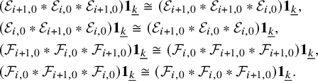 $$ \begin{align*} &(\mathcal{E}_{i+1,0} \ast \mathcal{E}_{i,0} \ast \mathcal{E}_{i+1,0})\boldsymbol{1}_{\underline{k}} \cong (\mathcal{E}_{i+1,0} \ast \mathcal{E}_{i+1,0} \ast \mathcal{E}_{i,0})\boldsymbol{1}_{\underline{k}}, \\ &(\mathcal{E}_{i,0} \ast \mathcal{E}_{i+1,0} \ast \mathcal{E}_{i,0})\boldsymbol{1}_{\underline{k}} \cong (\mathcal{E}_{i+1,0} \ast \mathcal{E}_{i,0} \ast \mathcal{E}_{i,0})\boldsymbol{1}_{\underline{k}}, \\ &(\mathcal{F}_{i+1,0} \ast \mathcal{F}_{i,0} \ast \mathcal{F}_{i+1,0})\boldsymbol{1}_{\underline{k}} \cong (\mathcal{F}_{i,0} \ast \mathcal{F}_{i+1,0} \ast \mathcal{F}_{i+1,0})\boldsymbol{1}_{\underline{k}}, \\ &(\mathcal{F}_{i,0} \ast \mathcal{F}_{i+1,0} \ast \mathcal{F}_{i,0})\boldsymbol{1}_{\underline{k}} \cong (\mathcal{F}_{i,0} \ast \mathcal{F}_{i,0} \ast \mathcal{F}_{i+1,0})\boldsymbol{1}_{\underline{k}}. \end{align*} $$
We are in a position to prove the Theorem 7.3.
Proof of Theorem 7.3.
For the proof of most relations, we will use the isomorphism
 $\mathcal {T}_{i} \cong (\mathcal {E}_{i,0} \ast \mathcal {F}_{i,1} \ast (\Psi ^{+}_{i})^{-1})\boldsymbol {1}_{(1,1,...,1)}$
from (7.13), since the argument for the other is similar.
$\mathcal {T}_{i} \cong (\mathcal {E}_{i,0} \ast \mathcal {F}_{i,1} \ast (\Psi ^{+}_{i})^{-1})\boldsymbol {1}_{(1,1,...,1)}$
from (7.13), since the argument for the other is similar.
First, we prove the relation (7.4). Then, we obtain
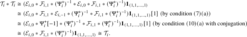 $$ \begin{align*} \mathcal{T}_{i} \ast \mathcal{T}_{i} & \cong (\mathcal{E}_{i,0} \ast \mathcal{F}_{i,1} \ast (\Psi^{+}_{i})^{-1} \ast \mathcal{E}_{i,0} \ast \mathcal{F}_{i,1} \ast (\Psi^{+}_{i})^{-1}) \boldsymbol{1}_{(1,1,...,1)} \\ & \cong (\mathcal{E}_{i,0} \ast \mathcal{F}_{i,1} \ast \mathcal{E}_{i,-1} \ast (\Psi^{+}_{i})^{-1} \ast \mathcal{F}_{i,1} \ast (\Psi^{+}_{i})^{-1}) \boldsymbol{1}_{(1,1,...,1)}[1] \ (\mathrm{by \ condition \ (7)(a)}) \\ & \cong (\mathcal{E}_{i,0} \ast \Psi^{+}_{i}[-1] \ast (\Psi^{+}_{i})^{-1} \ast \mathcal{F}_{i,1} \ast (\Psi^{+}_{i})^{-1}) \boldsymbol{1}_{(1,1,...,1)}[1] \ ({\mathrm{by \ condition \ (10)(a) \ with \ conjugation}}) \\ & \cong (\mathcal{E}_{i,0} \ast \mathcal{F}_{i,1} \ast (\Psi^{+}_{i})^{-1}) \boldsymbol{1}_{(1,1,...,1)} \cong \mathcal{T}_{i}. \end{align*} $$
Next, for relation (7.6), we let
 $j \neq i, i+1$
. Then, we use
$j \neq i, i+1$
. Then, we use
 $\mathcal {X}_{j} \cong \Psi ^{+}_{j-1}\boldsymbol {1}_{(1,1,...,1)}$
if
$\mathcal {X}_{j} \cong \Psi ^{+}_{j-1}\boldsymbol {1}_{(1,1,...,1)}$
if
 $i+2 \leq j \leq N$
and
$i+2 \leq j \leq N$
and
 $\mathcal {X}_{j} \cong (\Psi ^{-}_{j})^{-1}\boldsymbol {1}_{(1,1,...,1)}$
if
$\mathcal {X}_{j} \cong (\Psi ^{-}_{j})^{-1}\boldsymbol {1}_{(1,1,...,1)}$
if
 $1 \leq j \leq i-1$
. The result follows from conditions (4), (7)(b)(c), and (8)(b)(c) in Definition 3.1.
$1 \leq j \leq i-1$
. The result follows from conditions (4), (7)(b)(c), and (8)(b)(c) in Definition 3.1.
For relation (7.7) and (7.8), by conditions (10)(a)(b), we have the following exact triangles
 $$ \begin{align} &(\mathcal{F}_{i,1} \ast \mathcal{E}_{i,0})\boldsymbol{1}_{(1,1,...,1)} \rightarrow (\mathcal{E}_{i,0} \ast \mathcal{F}_{i,1})\boldsymbol{1}_{(1,1,....,1)} \rightarrow \Psi_{i}^{+}\boldsymbol{1}_{(1,1,...,1)} , \end{align} $$
 $$ \begin{align} &(\mathcal{E}_{i,-1} \ast \mathcal{F}_{i,0})\boldsymbol{1}_{(1,1,....,1)} \rightarrow (\mathcal{F}_{i,0} \ast \mathcal{E}_{i,-1})\boldsymbol{1}_{(1,1,...,1)} \rightarrow \Psi_{i}^{-}\boldsymbol{1}_{(1,1,...,1)}. \end{align} $$
Note that
 $(\mathcal {E}_{i,0} \ast \mathcal {F}_{i,1})\boldsymbol {1}_{(1,1,....,1)} \cong \mathcal {T}_{i} \ast \mathcal {X}_{i+1}$
since
$(\mathcal {E}_{i,0} \ast \mathcal {F}_{i,1})\boldsymbol {1}_{(1,1,....,1)} \cong \mathcal {T}_{i} \ast \mathcal {X}_{i+1}$
since
 $\mathcal {T}_{i} \cong (\mathcal {E}_{i,0} \ast \mathcal {F}_{i,1} \ast (\Psi ^{+}_{i})^{-1})\boldsymbol {1}_{(1,1,...,1)}$
and
$\mathcal {T}_{i} \cong (\mathcal {E}_{i,0} \ast \mathcal {F}_{i,1} \ast (\Psi ^{+}_{i})^{-1})\boldsymbol {1}_{(1,1,...,1)}$
and
 $\mathcal {X}_{i+1} \cong \Psi ^{+}_{i}\boldsymbol {1}_{(1,1,...,1)}$
. On the other hand,
$\mathcal {X}_{i+1} \cong \Psi ^{+}_{i}\boldsymbol {1}_{(1,1,...,1)}$
. On the other hand,
 $\mathcal {T}_{i} \cong (\mathcal {F}_{i,0} \ast \mathcal {E}_{i,0})\boldsymbol {1}_{(1,1,...,1)}$
by (7.9) and
$\mathcal {T}_{i} \cong (\mathcal {F}_{i,0} \ast \mathcal {E}_{i,0})\boldsymbol {1}_{(1,1,...,1)}$
by (7.9) and
 $\mathcal {X}_{i} \cong (\Psi ^{-}_{i})^{-1}\boldsymbol {1}_{(1,1,...,1)}$
, thus
$\mathcal {X}_{i} \cong (\Psi ^{-}_{i})^{-1}\boldsymbol {1}_{(1,1,...,1)}$
, thus
 $$ \begin{align*} \mathcal{X}_{i} \ast \mathcal{T}_{i} \cong ((\Psi^{-}_{i})^{-1} \ast \mathcal{F}_{i,0} \ast \mathcal{E}_{i,0})\boldsymbol{1}_{(1,1,...,1)} \cong ( \mathcal{F}_{i,1} \ast (\Psi^{-}_{i})^{-1} \ast \mathcal{E}_{i,0})\boldsymbol{1}_{(1,1,...,1)}[1] \cong (\mathcal{F}_{i,1}\ast \mathcal{E}_{i,0})\boldsymbol{1}_{(1,1,...,1)} \end{align*} $$
where we use condition (8)(a) in the second isomorphism and the third isomorphism comes from the fact that the kernel
 $\Psi ^{-}_{i}\boldsymbol {1}_{(1,1,...,1)+\alpha _{i}}$
is given by
$\Psi ^{-}_{i}\boldsymbol {1}_{(1,1,...,1)+\alpha _{i}}$
is given by
 $\mathcal {O}_{\Delta }[1]$
. With these facts, the exact triangle (7.14) is precisely the following
$\mathcal {O}_{\Delta }[1]$
. With these facts, the exact triangle (7.14) is precisely the following
 $$ \begin{align*} \mathcal{X}_{i} \ast \mathcal{T}_{i} \rightarrow \mathcal{T}_{i} \ast \mathcal{X}_{i+1} \rightarrow \mathcal{X}_{i+1} \end{align*} $$
which is the relation (7.8). A similar argument with the exact triangle (7.15) gives the relation (7.7).
Finally, we prove the braid relation in (7.5).
For the non-adjacent relation, it follows from conditions (4), (5)(c), (6)(c), (7)(c), (8)(c), and (9) in Definition 3.1.
Since
 $\mathcal {T}_{i} \cong (\mathcal {E}_{i,0} \ast \mathcal {F}_{i,0})\boldsymbol {1}_{(1,1,...,1)} \cong (\mathcal {F}_{i,0} \ast \mathcal {E}_{i,0})\boldsymbol {1}_{(1,1,...,1)}$
by (7.9), a direct calculation shows that
$\mathcal {T}_{i} \cong (\mathcal {E}_{i,0} \ast \mathcal {F}_{i,0})\boldsymbol {1}_{(1,1,...,1)} \cong (\mathcal {F}_{i,0} \ast \mathcal {E}_{i,0})\boldsymbol {1}_{(1,1,...,1)}$
by (7.9), a direct calculation shows that
 $$ \begin{align} \mathcal{T}_{i}\ast \mathcal{T}_{i+1} \ast \mathcal{T}_{i} & \cong (\mathcal{E}_{i,0} \ast \mathcal{F}_{i,0} \ast \mathcal{E}_{i+1,0} \ast \mathcal{F}_{i+1,0} \ast \mathcal{E}_{i,0} \ast \mathcal{F}_{i,0}) \boldsymbol{1}_{(1,1,...,1)} \nonumber\\ & \cong (\mathcal{E}_{i,0} \ast \mathcal{E}_{i+1,0} \ast \mathcal{F}_{i,0} \ast \mathcal{E}_{i,0} \ast \mathcal{F}_{i+1,0} \ast \mathcal{F}_{i,0}) \boldsymbol{1}_{(1,1,...,1)} \ (\text{by} \ \text{condition (9)}) \nonumber \\ & \cong (\mathcal{E}_{i,0} \ast \mathcal{E}_{i+1,0} \ast \mathcal{E}_{i,0} \ast \mathcal{F}_{i,0} \ast \mathcal{F}_{i+1,0} \ast \mathcal{F}_{i,0}) \boldsymbol{1}_{(1,1,...,1)} \ (\text{by} \ \text{condition (10)(c)}) \nonumber\\ & \cong (\mathcal{E}_{i+1,0} \ast \mathcal{E}_{i,0} \ast \mathcal{E}_{i,0} \ast \mathcal{F}_{i,0} \ast \mathcal{F}_{i,0} \ast \mathcal{F}_{i+1,0})\boldsymbol{1}_{(1,1,...,1)} \ (\text{by} \ \text{Lemma} \ 7.4) \nonumber\\ & \cong (\mathcal{E}_{i+1,0} \ast \mathcal{E}_{i,0} \ast \mathcal{F}_{i,0} \ast \mathcal{E}_{i,0} \ast \mathcal{F}_{i,0} \ast \mathcal{F}_{i+1,0})\boldsymbol{1}_{(1,1,...,1)}{.} \ (\text{by} \ \text{condition (10)(c)}) \end{align} $$
Next, we show that
 $(\mathcal {E}_{i,0} \ast \mathcal {F}_{i,0} \ast \mathcal {E}_{i,0} \ast \mathcal {F}_{i,0})\boldsymbol {1}_{(1,1,...,1)-\alpha _{i+1}} \cong (\mathcal {E}_{i,0} \ast \mathcal {F}_{i,0})\boldsymbol {1}_{(1,1,...,1)-\alpha _{i+1}}$
. First, we observe that
$(\mathcal {E}_{i,0} \ast \mathcal {F}_{i,0} \ast \mathcal {E}_{i,0} \ast \mathcal {F}_{i,0})\boldsymbol {1}_{(1,1,...,1)-\alpha _{i+1}} \cong (\mathcal {E}_{i,0} \ast \mathcal {F}_{i,0})\boldsymbol {1}_{(1,1,...,1)-\alpha _{i+1}}$
. First, we observe that
 $(\mathcal {E}_{i,0} \ast \mathcal {F}_{i,0})\boldsymbol {1}_{(1,1,...,1)-\alpha _{i+1}} \cong (\mathcal {F}_{i,0} \ast \mathcal {E}_{i,0})\boldsymbol {1}_{(1,1,...,1)-\alpha _{i+1}}$
. Then by condition (7)(a), we get
$(\mathcal {E}_{i,0} \ast \mathcal {F}_{i,0})\boldsymbol {1}_{(1,1,...,1)-\alpha _{i+1}} \cong (\mathcal {F}_{i,0} \ast \mathcal {E}_{i,0})\boldsymbol {1}_{(1,1,...,1)-\alpha _{i+1}}$
. Then by condition (7)(a), we get
 $$ \begin{align*} (\mathcal{F}_{i,0} \ast \mathcal{E}_{i,0})\boldsymbol{1}_{(1,1,...,1)-\alpha_{i+1}} &\cong (\mathcal{F}_{i,0} \ast \Psi_{i}^{-} \ast \mathcal{E}_{i,-1} \ast (\Psi_{i}^{-})^{-1} )\boldsymbol{1}_{(1,1,...,1)-\alpha_{i+1}}[-1] \\ & \cong (\mathcal{F}_{i,0} \ast \mathcal{E}_{i,-1} \ast (\Psi_{i}^{-})^{-1} )\boldsymbol{1}_{(1,1,...,1)-\alpha_{i+1}} \end{align*} $$
where the second isomorphism comes from the fact that
 $\Psi _{i}^{-}\boldsymbol {1}_{(1,1,...,1)-\alpha _{i+1}+\alpha _{i}}$
is given by
$\Psi _{i}^{-}\boldsymbol {1}_{(1,1,...,1)-\alpha _{i+1}+\alpha _{i}}$
is given by
 $\mathcal {O}_{\Delta }[1]$
. Thus
$\mathcal {O}_{\Delta }[1]$
. Thus
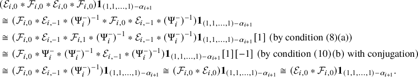 $$ \begin{align*} &(\mathcal{E}_{i,0} \ast \mathcal{F}_{i,0} \ast \mathcal{E}_{i,0} \ast \mathcal{F}_{i,0})\boldsymbol{1}_{(1,1,...,1)-\alpha_{i+1}} \\ &\cong (\mathcal{F}_{i,0} \ast \mathcal{E}_{i,-1} \ast (\Psi_{i}^{-})^{-1} \ast \mathcal{F}_{i,0} \ast \mathcal{E}_{i,-1} \ast (\Psi_{i}^{-})^{-1} )\boldsymbol{1}_{(1,1,...,1)-\alpha_{i+1}} \\ & \cong (\mathcal{F}_{i,0} \ast \mathcal{E}_{i,-1} \ast \mathcal{F}_{i,1} \ast (\Psi_{i}^{-})^{-1} \ast \mathcal{E}_{i,-1} \ast (\Psi_{i}^{-})^{-1} )\boldsymbol{1}_{(1,1,...,1)-\alpha_{i+1}}[1] \ (\text{by} \ \text{condition (8)(a)}) \\ & \cong (\mathcal{F}_{i,0} \ast \Psi_{i}^{-} \ast (\Psi_{i}^{-})^{-1} \ast \mathcal{E}_{i,-1} \ast (\Psi_{i}^{-})^{-1} )\boldsymbol{1}_{(1,1,...,1)-\alpha_{i+1}}[1][-1] \ (\mathrm{{by \ condition \ (10)(b) \ with \ conjugation}}) \\ & \cong (\mathcal{F}_{i,0} \ast \mathcal{E}_{i,-1} \ast (\Psi_{i}^{-})^{-1} )\boldsymbol{1}_{(1,1,...,1)-\alpha_{i+1}} \cong (\mathcal{F}_{i,0} \ast \mathcal{E}_{i,0})\boldsymbol{1}_{(1,1,...,1)-\alpha_{i+1}} \cong (\mathcal{E}_{i,0} \ast \mathcal{F}_{i,0})\boldsymbol{1}_{(1,1,...,1)-\alpha_{i+1}}. \end{align*} $$
So (7.16) becomes
 $$ \begin{align} (\mathcal{E}_{i+1,0} \ast \mathcal{E}_{i,0} \ast \mathcal{F}_{i,0} \ast \mathcal{F}_{i+1,0})\boldsymbol{1}_{(1,1,...,1)} & \cong (\mathcal{E}_{i+1,0} \ast \mathcal{F}_{i,0} \ast \mathcal{E}_{i,0} \ast \mathcal{F}_{i+1,0})\boldsymbol{1}_{(1,1,...,1)} \nonumber\\ & \cong (\mathcal{F}_{i,0} \ast \mathcal{E}_{i+1,0} \ast \mathcal{F}_{i+1,0} \ast \mathcal{E}_{i,0})\boldsymbol{1}_{(1,1,...,1)}. \end{align} $$
Using the same argument, we can show that
 $(\mathcal {E}_{i+1,0} \ast \mathcal {F}_{i+1,0})\boldsymbol {1}_{(1,1,...,1)+\alpha _{i}} \cong (\mathcal {E}_{i+1,0} \ast \mathcal {F}_{i+1,0} \ast \mathcal {E}_{i+1,0} \ast \mathcal {F}_{i+1,0})\boldsymbol {1}_{(1,1,...,1)+\alpha _{i}}$
. Hence (7.17) becomes
$(\mathcal {E}_{i+1,0} \ast \mathcal {F}_{i+1,0})\boldsymbol {1}_{(1,1,...,1)+\alpha _{i}} \cong (\mathcal {E}_{i+1,0} \ast \mathcal {F}_{i+1,0} \ast \mathcal {E}_{i+1,0} \ast \mathcal {F}_{i+1,0})\boldsymbol {1}_{(1,1,...,1)+\alpha _{i}}$
. Hence (7.17) becomes
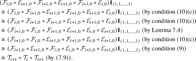 $$ \begin{align*} &(\mathcal{F}_{i,0} \ast \mathcal{E}_{i+1,0} \ast \mathcal{F}_{i+1,0} \ast \mathcal{E}_{i+1,0} \ast \mathcal{F}_{i+1,0} \ast \mathcal{E}_{i,0})\boldsymbol{1}_{(1,1,...,1)} \\ &\cong (\mathcal{F}_{i,0} \ast \mathcal{F}_{i+1,0} \ast \mathcal{E}_{i+1,0} \ast \mathcal{F}_{i+1,0} \ast \mathcal{E}_{i+1,0} \ast \mathcal{E}_{i,0})\boldsymbol{1}_{(1,1,...,1)} \ (\text{by} \ \text{condition (10)(c)}) \\ &\cong (\mathcal{F}_{i,0} \ast \mathcal{F}_{i+1,0} \ast \mathcal{F}_{i+1,0} \ast \mathcal{E}_{i+1,0} \ast \mathcal{E}_{i+1,0} \ast \mathcal{E}_{i,0})\boldsymbol{1}_{(1,1,...,1)} \ (\text{by} \ \text{condition (10)(c)}) \\ & \cong (\mathcal{F}_{i+1,0} \ast \mathcal{F}_{i,0} \ast \mathcal{F}_{i+1,0} \ast \mathcal{E}_{i+1,0} \ast \mathcal{E}_{i,0} \ast \mathcal{E}_{i+1,0})\boldsymbol{1}_{(1,1,...,1)} \ (\text{by} \ \text{Lemma} \ 7.4) \\ & \cong (\mathcal{F}_{i+1,0} \ast \mathcal{F}_{i,0} \ast \mathcal{E}_{i+1,0} \ast \mathcal{F}_{i+1,0} \ast \mathcal{E}_{i,0} \ast \mathcal{E}_{i+1,0})\boldsymbol{1}_{(1,1,...,1)} \ (\text{by} \ \text{condition (10)(c)}) \\ & \cong (\mathcal{F}_{i+1,0} \ast \mathcal{E}_{i+1,0} \ast \mathcal{F}_{i,0} \ast \mathcal{E}_{i,0} \ast \mathcal{F}_{i+1,0} \ast \mathcal{E}_{i+1,0})\boldsymbol{1}_{(1,1,...,1)} \ (\text{by} \ \text{condition (9)}) \\ & \cong \mathcal{T}_{i+1}\ast \mathcal{T}_{i} \ast \mathcal{T}_{i+1} \ (\text{by} \ (7.9)).\\[-37pt] \end{align*} $$
We give a few remarks to conclude this section.
Remark 7.5. We explain why we prefer (7.13) over (7.9) for writing the categorified Demazure operators in terms of 1-morphisms in the categorical
 $\mathcal {U}$
-action. The main reason comes from the naturality of adjoint functors, i.e., condition (3).
$\mathcal {U}$
-action. The main reason comes from the naturality of adjoint functors, i.e., condition (3).
By condition (3), we obtain that
 $$ \begin{align*} \mathrm{Hom}({\mathcal{E}}_{i,0}\boldsymbol{1}_{(1,1,...,1)-\alpha_{i}}, {\mathcal{E}}_{i,0}\boldsymbol{1}_{(1,1,...,1)-\alpha_{i}}) &\cong \mathrm{Hom}(\boldsymbol{1}_{(1,1,...,1)}{\mathcal{E}}_{i,0} \ast ({\mathcal{E}}_{i,0}\boldsymbol{1}_{(1,1,...,1)-\alpha_{i}})_{R}, \boldsymbol{1}_{(1,1,...,1)}) \\ & \cong \mathrm{Hom}(({\mathcal{E}}_{i,0} \ast{\mathcal{F}}_{i,1} \ast({\Psi}^{+}_{i})^{-1})\boldsymbol{1}_{(1,1,...,1)}, \boldsymbol{1}_{(1,1,...,1)}). \end{align*} $$
Thus,
 $({\mathcal {E}}_{i,0} \ast {\mathcal {F}}_{i,1} \ast ({\Psi }^{+}_{i})^{-1})\boldsymbol {1}_{(1,1,...,1)}$
naturally appears as the kernel for the composition of adjoint functors
$({\mathcal {E}}_{i,0} \ast {\mathcal {F}}_{i,1} \ast ({\Psi }^{+}_{i})^{-1})\boldsymbol {1}_{(1,1,...,1)}$
naturally appears as the kernel for the composition of adjoint functors
 $\mathsf {E}_{i,0} \circ (\mathsf {E}_{i,0}\boldsymbol {1}_{(1,1,...,1)-\alpha _{i}})^{R}\boldsymbol {1}_{(1,1,...,1)}$
. Similarly, we also have
$\mathsf {E}_{i,0} \circ (\mathsf {E}_{i,0}\boldsymbol {1}_{(1,1,...,1)-\alpha _{i}})^{R}\boldsymbol {1}_{(1,1,...,1)}$
. Similarly, we also have
 $({\mathcal {F}}_{i,0} \ast {\mathcal {E}}_{i,-1} \ast ({\Psi }^{-}_{i})^{-1})\boldsymbol {1}_{(1,1,...,1)}$
naturally appearing as the kernel for the composition of adjoint functors
$({\mathcal {F}}_{i,0} \ast {\mathcal {E}}_{i,-1} \ast ({\Psi }^{-}_{i})^{-1})\boldsymbol {1}_{(1,1,...,1)}$
naturally appearing as the kernel for the composition of adjoint functors
 $\mathsf {F}_{i,0} \circ (\mathsf {F}_{i,0}\boldsymbol {1}_{(1,1,...,1)+\alpha _{i}})^{R}\boldsymbol {1}_{(1,1,...,1)}$
.
$\mathsf {F}_{i,0} \circ (\mathsf {F}_{i,0}\boldsymbol {1}_{(1,1,...,1)+\alpha _{i}})^{R}\boldsymbol {1}_{(1,1,...,1)}$
.
Moreover, we expect that the morphisms in the exact triangles (7.14) and (7.15) should be determined to come from the identity morphisms
 $Id:{\mathcal {E}}_{i,0}\boldsymbol {1}_{(1,1,...,1)-\alpha _{i}} \rightarrow {\mathcal {E}}_{i,0}\boldsymbol {1}_{(1,1,...,1)-\alpha _{i}}$
and
$Id:{\mathcal {E}}_{i,0}\boldsymbol {1}_{(1,1,...,1)-\alpha _{i}} \rightarrow {\mathcal {E}}_{i,0}\boldsymbol {1}_{(1,1,...,1)-\alpha _{i}}$
and
 $Id:{\mathcal {F}}_{i,0}\boldsymbol {1}_{(1,1,...,1)+\alpha _{i}} \rightarrow {\mathcal {F}}_{i,0}\boldsymbol {1}_{(1,1,...,1)+\alpha _{i}}$
, respectively.
$Id:{\mathcal {F}}_{i,0}\boldsymbol {1}_{(1,1,...,1)+\alpha _{i}} \rightarrow {\mathcal {F}}_{i,0}\boldsymbol {1}_{(1,1,...,1)+\alpha _{i}}$
, respectively.
Remark 7.6. In [Reference Hsu26], we generalize the interpretation of categorified Demazure operators in terms of the 1-morphisms in the categorical
 $\mathcal {U}$
-action, i.e. (7.13), from the full flag variety
$\mathcal {U}$
-action, i.e. (7.13), from the full flag variety
 $G/B$
to the n-step partial flag varieties
$G/B$
to the n-step partial flag varieties
 $\mathrm {Fl}_{\underline {k}}(\mathbb {C}^N)$
. More precisely, we construct two families of pairs of complementary idempotents in
$\mathrm {Fl}_{\underline {k}}(\mathbb {C}^N)$
. More precisely, we construct two families of pairs of complementary idempotents in
 $\mathrm {D}^b(\mathrm {Fl}_{\underline {k}}(\mathbb {C}^N) \times \mathrm {Fl}_{\underline {k}}(\mathbb {C}^N))$
acting on
$\mathrm {D}^b(\mathrm {Fl}_{\underline {k}}(\mathbb {C}^N) \times \mathrm {Fl}_{\underline {k}}(\mathbb {C}^N))$
acting on
 $\mathrm {D}^b(\mathrm {Fl}_{\underline {k}}(\mathbb {C}^N))$
. Moreover, those complementary idempotents provide short semiorthogonal decompositions of
$\mathrm {D}^b(\mathrm {Fl}_{\underline {k}}(\mathbb {C}^N))$
. Moreover, those complementary idempotents provide short semiorthogonal decompositions of
 $\mathrm {D}^b(\mathrm {Fl}_{\underline {k}}(\mathbb {C}^N))$
, and we determine the generators of the component categories in the Grassmannians case. Finally, we also give another proof of the braid relation (7.5) in Theorem 7.3 which is shorter than the one in this article.
$\mathrm {D}^b(\mathrm {Fl}_{\underline {k}}(\mathbb {C}^N))$
, and we determine the generators of the component categories in the Grassmannians case. Finally, we also give another proof of the braid relation (7.5) in Theorem 7.3 which is shorter than the one in this article.
Remark 7.7. We try to relate categorical actions of affine 0-Hecke algebras to the notion of Demazure descent data on a triangulated category defined in [Reference Arkhipov and Kanstrup2], [Reference Arkhipov and Kanstrup3].
From (7.5) in Theorem 7.3, we know that those FM kernels
 $\{\mathcal {T}_{i}\}_{1 \leq i \leq N-1}$
give a weak braid monoid action on
$\{\mathcal {T}_{i}\}_{1 \leq i \leq N-1}$
give a weak braid monoid action on
 $\mathrm {D}^b(G/B)$
. Moreover, (7.4) in Theorem 7.3 implies that there is a co-projector structure on
$\mathrm {D}^b(G/B)$
. Moreover, (7.4) in Theorem 7.3 implies that there is a co-projector structure on
 $\mathcal {T}_{i}$
for all i. Thus
$\mathcal {T}_{i}$
for all i. Thus
 $\{\mathcal {T}_{i}\}_{1 \leq i \leq N-1}$
gives a Demazure descent data on
$\{\mathcal {T}_{i}\}_{1 \leq i \leq N-1}$
gives a Demazure descent data on
 $\mathrm {D}^b(G/B)$
.
$\mathrm {D}^b(G/B)$
.
A A Conjectural Presentation
In this appendix, we define another algebra which can be viewed as a second definition of the shifted 0-affine algebra. It has the so-called loop presentation that given by using generating series. Thus, in this definition, we have infinite generators and relations.
Then, we construct an action of this algebra on the Grothendieck groups of n-step partial flag varieties
 $\bigoplus _{\underline {k}}K(\mathrm {Fl}_{\underline {k}}(\mathbb {C}^N))$
.
$\bigoplus _{\underline {k}}K(\mathrm {Fl}_{\underline {k}}(\mathbb {C}^N))$
.
Finally, we conjecture that the loop presentation we defined for the shifted 0-affine algebra is equivalent to the presentation defined in Definition 2.6.
Definition A.1. Defining the associative
 $\mathbb {C}$
-algebra
$\mathbb {C}$
-algebra
 $\dot {\mathrm {\mathbf {U}}}^{\prime }_{0,N}(L\mathfrak {sl}_n)$
that is generated by
$\dot {\mathrm {\mathbf {U}}}^{\prime }_{0,N}(L\mathfrak {sl}_n)$
that is generated by
 $$ \begin{align*} \bigcup_{\underline{k} \in C(n,N)} \{1_{\underline{k}}, \ 1_{\underline{k}+\alpha_{i}}e_{i,r}1_{\underline{k}}, \ 1_{\underline{k}-\alpha_{i}}f_{i,r}1_{\underline{k}}, \ 1_{\underline{k}}\psi^{\pm}_{i,\pm s^{\pm}_{i}}1_{\underline{k}}, \ 1_{\underline{k}}(\psi^{+}_{i,k_{i+1}})^{-1}1_{\underline{k}}, \ 1_{\underline{k}}(\psi^{-}_{i,-k_{i}})^{-1}1_{\underline{k}} \}_{1 \leq i \leq n-1}^{r \in \mathbb{Z}, \ s^{+}_{i} \geq k_{i+1}, \ s^{-}_{i} \geq k_{i}} \end{align*} $$
with the following relations (for all
 $1\leq i,j \leq n-1$
,
$1\leq i,j \leq n-1$
,
 $\underline {k} \in C(n,N)$
,
$\underline {k} \in C(n,N)$
,
 $\epsilon ,\epsilon ' \in \{\pm \}$
and
$\epsilon ,\epsilon ' \in \{\pm \}$
and
 $s^{+}_{i} \geq k_{i+1}$
,
$s^{+}_{i} \geq k_{i+1}$
,
 $s^{-}_{i} \geq k_{i}$
).
$s^{-}_{i} \geq k_{i}$
).
 $$ \begin{align} 1_{\underline{k}}1_{\underline{l}}=\delta_{\underline{k},\underline{l}}1_{\underline{k}}, \end{align} $$
 $$ \begin{align} [\psi^{\epsilon}_{i,\underline{k}}(z), \psi^{\epsilon'}_{j,\underline{k}}(w)]1_{\underline{k}}=0, \ (\psi^{+}_{i,k_{i+1}})^{\pm 1} \cdot (\psi^{+}_{i,k_{i+1}})^{\mp 1} 1_{\underline{k}} = 1_{\underline{k}}=(\psi^{-}_{i,-k_{i}})^{\pm 1} \cdot (\psi^{-}_{i,-k_{i}})^{\mp 1}1_{\underline{k}}. \end{align} $$
 $$ \begin{align} &ze_{i,\underline{k}+\alpha_{i}}(z)e_{i,\underline{k}}(w)1_{\underline{k}}=-we_{i,\underline{k}+\alpha_{i}}(w)e_{i,\underline{k}}(z)1_{\underline{k}}, \nonumber \\ &we_{i,\underline{k}+\alpha_{i+1}}(z)e_{i+1,\underline{k}}(w)1_{\underline{k}}=(w-z)e_{i+1,\underline{k}+\alpha_{i}}(w)e_{i,\underline{k}}(z)1_{\underline{k}}, \\ & \nonumber (z-w)e_{i,\underline{k}+\alpha_{j}}(z)e_{j,\underline{k}}(w)1_{\underline{k}}=(z-w)e_{j,\underline{k}+\alpha_{i}}(w)e_{i,\underline{k}}(z)1_{\underline{k}}, \ \text{if} \ |i-j| \geq 2. \end{align} $$
 $$ \begin{align} &-wf_{i,\underline{k}-\alpha_{i}}(z)f_{i,\underline{k}}(w)1_{\underline{k}}=zf_{i,\underline{k}-\alpha_{i}}(w)f_{i,\underline{k}}(z)1_{\underline{k}}, \nonumber \\ &(w-z)f_{i,\underline{k}-\alpha_{i+1}}(z)f_{i+1,\underline{k}}(w)1_{\underline{k}}=wf_{i+1,\underline{k}-\alpha_{i}}(w)f_{i,\underline{k}}(z)1_{\underline{k}}, \\ &(z-w)f_{i,\underline{k}-\alpha_{j}}(z)f_{j,\underline{k}}(w)1_{\underline{k}}=(z-w)f_{j,\underline{k}-\alpha_{i}}(w)f_{i,\underline{k}}(z)1_{\underline{k}}, \ \text{if} \ |i-j| \geq 2.\nonumber \end{align} $$
 $$ \begin{align} &z\psi^{+}_{i,\underline{k}+\alpha_{i}}(z)e_{i,\underline{k}}(w)1_{\underline{k}}=-we_{i,\underline{k}}(w)\psi^{+}_{i,\underline{k}}(z)1_{\underline{k}}, \nonumber\\ &\frac{-w}{z}(\sum_{s \geq 0}(\frac{w}{z})^s)\psi^{+}_{i,\underline{k}+\alpha_{i+1}}(z)e_{i+1,\underline{k}}(w)1_{\underline{k}}=e_{i+1,\underline{k}}(w)\psi^{+}_{i,\underline{k}}(z)1_{\underline{k}}, \nonumber\\ &\psi^{+}_{i,\underline{k}+\alpha_{i-1}}(z)e_{i-1,\underline{k}}(w)1_{\underline{k}}=(\sum_{s \geq 0}(\frac{w}{z})^s)e_{i-1,\underline{k}}(w)\psi^{+}_{i,\underline{k}}(z)1_{\underline{k}}, \\ &\psi^{+}_{i,\underline{k}+\alpha_{j}}(z)e_{j,\underline{k}}(w)1_{\underline{k}}=e_{j,\underline{k}}(w)\psi^{+}_{i,\underline{k}}(z)1_{\underline{k}}, \ \text{if} \ |i-j| \geq 2.\nonumber \end{align} $$
 $$ \begin{align} &z\psi^{-}_{i,\underline{k}+\alpha_{i}}(z)e_{i,\underline{k}}(w)1_{\underline{k}}=-we_{i,\underline{k}}(w)\psi^{-}_{i,\underline{k}}(z)1_{\underline{k}}, \nonumber\\ &(\sum_{s \geq 0}(\frac{z}{w})^s)\psi^{-}_{i,\underline{k}+\alpha_{i+1}}(z)e_{i+1,\underline{k}}(w)1_{\underline{k}}=e_{i+1,\underline{k}}(w)\psi^{-}_{i,\underline{k}}(z)1_{\underline{k}},\nonumber \\ &\psi^{-}_{i,\underline{k}+\alpha_{i-1}}(z)e_{i-1,\underline{k}}(w)1_{\underline{k}}=\frac{-z}{w}(\sum_{s \geq 0}(\frac{z}{w})^s)e_{i-1,\underline{k}}(w)\psi^{-}_{i,\underline{k}}(z)1_{\underline{k}},\\ &\psi^{-}_{i,\underline{k}+\alpha_{j}}(z)e_{j,\underline{k}}(w)1_{\underline{k}}=e_{j,\underline{k}}(w)\psi^{-}_{i,\underline{k}}(z)1_{\underline{k}}, \ \text{if} \ |i-j| \geq 2.\nonumber \end{align} $$
 $$ \begin{align} &-w\psi^{+}_{i,\underline{k}-\alpha_{i}}(z)f_{i,\underline{k}}(w)1_{\underline{k}}=zf_{i,\underline{k}}(w)\psi^{+}_{i,\underline{k}}(z)1_{\underline{k}}, \nonumber\\ &\psi^{+}_{i,\underline{k}-\alpha_{i+1}}(z)f_{i+1,\underline{k}}(w)1_{\underline{k}}=\frac{-w}{z}(\sum_{s \geq 0}(\frac{w}{z})^s)f_{i+1,\underline{k}}(w)\psi^{+}_{i,\underline{k}}(z)1_{\underline{k}}, \nonumber\\ &(\sum_{s \geq 0}(\frac{w}{z})^s)\psi^{+}_{i,\underline{k}-\alpha_{i-1}}(z)f_{i-1,\underline{k}}(w)1_{\underline{k}}=f_{i-1,\underline{k}}(w)\psi^{+}_{i,\underline{k}}(z)1_{\underline{k}}, \\ &\psi^{+}_{i,\underline{k}-\alpha_{j}}(z)f_{j,\underline{k}}(w)1_{\underline{k}}=f_{j,\underline{k}}(w)\psi^{+}_{i,\underline{k}}(z)1_{\underline{k}}, \ \text{if} \ |i-j| \geq 2.\nonumber \end{align} $$
 $$ \begin{align} &-w\psi^{-}_{i,\underline{k}-\alpha_{i}}(z)f_{i,\underline{k}}(w)1_{\underline{k}}=zf_{i,\underline{k}}(w)\psi^{-}_{i,\underline{k}}(z)1_{\underline{k}}, \nonumber \\ &\psi^{-}_{i,\underline{k}-\alpha_{i+1}}(z)f_{i+1,\underline{k}}(w)1_{\underline{k}}=(\sum_{s \geq 0}(\frac{z}{w})^s)f_{i+1,\underline{k}}(w)\psi^{-}_{i,\underline{k}}(z)1_{\underline{k}}, \nonumber\\ &\frac{-z}{w}(\sum_{s \geq 0}(\frac{z}{w})^s)\psi^{-}_{i,\underline{k}-\alpha_{i-1}}(z)f_{i-1,\underline{k}}(w)1_{\underline{k}}=f_{i-1,\underline{k}}(w)\psi^{-}_{i,\underline{k}}(z)1_{\underline{k}}, \\ &\psi^{-}_{i,\underline{k}-\alpha_{j}}(z)f_{j,\underline{k}}(w)1_{\underline{k}}=f_{j,\underline{k}}(w)\psi^{-}_{i,\underline{k}}(z)1_{\underline{k}}, \ \text{if} \ |i-j| \geq 2.\nonumber \end{align} $$
 $$ \begin{align} e_{i,\underline{k}-\alpha_{i}}(z)f_{i,\underline{k}}(w)1_{\underline{k}}-f_{i,\underline{k}+\alpha_{i}}(w)e_{i,\underline{k}}(z)1_{\underline{k}}=\delta_{ij}\delta(\frac{z}{w})(\psi^{+}_{i,\underline{k}}(z)-\psi^{-}_{i,\underline{k}}(z))1_{\underline{k}}. \end{align} $$
where the generating series are defined as follows
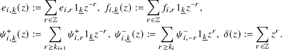 $$\begin{align*}e_{i,\underline{k}}(z)&:=\sum_{r \in \mathbb{Z}} e_{i,r}1_{\underline{k}}z^{-r},\ f_{i,\underline{k}}(z):=\sum_{r \in \mathbb{Z}} f_{i,r}1_{\underline{k}}z^{-r},\\\psi^{+}_{i,\underline{k}}(z)&:=\sum_{r \geq k_{i+1}} \psi^{+}_{i,r}1_{\underline{k}}z^{-r}, \ \psi^{-}_{i,\underline{k}}(z):=\sum_{r \geq k_{i}} \psi^{-}_{i,-r}1_{\underline{k}}z^{r}, \ \delta(z):=\sum_{r\in \mathbb{Z}} z^r. \end{align*}$$
Although the notion of categorical action of
 $\dot {\mathrm {\mathbf {U}}}^{\prime }_{0,N}(L\mathfrak {sl}_n)$
is not easy to define, we can construct an action on the Grothendieck groups of n-step partial flag varieties
$\dot {\mathrm {\mathbf {U}}}^{\prime }_{0,N}(L\mathfrak {sl}_n)$
is not easy to define, we can construct an action on the Grothendieck groups of n-step partial flag varieties
 $\mathrm {Fl}_{\underline {k}}(\mathbb {C}^N)$
.
$\mathrm {Fl}_{\underline {k}}(\mathbb {C}^N)$
.
To construct such action, we have to define the action of those generators in
 $\dot {\mathrm {\mathbf {U}}}^{\prime }_{0,N}(L\mathfrak {sl}_n)$
. First, we define
$\dot {\mathrm {\mathbf {U}}}^{\prime }_{0,N}(L\mathfrak {sl}_n)$
. First, we define
 $e_{i,r}1_{\underline {k}}$
and
$e_{i,r}1_{\underline {k}}$
and
 $f_{i,s}1_{\underline {k}}$
for all
$f_{i,s}1_{\underline {k}}$
for all
 $r,s \in \mathbb {Z}$
via using the K-theoretic FM transforms, i.e.,
$r,s \in \mathbb {Z}$
via using the K-theoretic FM transforms, i.e.,
 $$ \begin{align*} e_{i,r}1_{\underline{k}}:K(\mathrm{Fl}_{\underline{k}}(\mathbb{C}^N)) \rightarrow K(\mathrm{Fl}_{\underline{k}+\alpha_{i}}(\mathbb{C}^N)), \ x \mapsto \pi_{2*}(\pi^{*}_{1}(x) \otimes [\iota(\underline{k})_{*}(\mathcal{V}_{i}/\mathcal{V}^{\prime}_{i})^{\otimes r}]) \end{align*} $$
for all
 $r \in \mathbb {Z}$
, and similarly for
$r \in \mathbb {Z}$
, and similarly for
 $f_{i,s}1_{\underline {k}}$
in the opposite direction with
$f_{i,s}1_{\underline {k}}$
in the opposite direction with
 $s \in \mathbb {Z}$
. Next, for
$s \in \mathbb {Z}$
. Next, for
 $\psi ^{\pm }_{i, \pm s_{i}^{\pm }}1_{\underline {k}}$
we define their action on
$\psi ^{\pm }_{i, \pm s_{i}^{\pm }}1_{\underline {k}}$
we define their action on
 $K(\mathrm {Fl}_{\underline {k}}(\mathbb {C}^N))$
as the follows
$K(\mathrm {Fl}_{\underline {k}}(\mathbb {C}^N))$
as the follows
 $$ \begin{align} \psi^{+}_{i, s_{i}^{+}}1_{\underline{k}}:&K(\mathrm{Fl}_{\underline{k}}(\mathbb{C}^N)) \rightarrow K(\mathrm{Fl}_{\underline{k}}(\mathbb{C}^N)), \nonumber\\ & x \mapsto x \otimes (-1)^{k_{i+1}-1}[\det(\mathcal{V}_{i+1}/\mathcal{V}_{i})][\mathrm{Sym}^{s^{+}_{i}-k_{i+1}}(\mathcal{V}_{i+1}/\mathcal{V}_{i-1})] \end{align} $$
where
 $s^{+}_{i} \geq k_{i+1}$
and similarly
$s^{+}_{i} \geq k_{i+1}$
and similarly
 $$ \begin{align} \psi^{-}_{i, -s_{i}^{-}}1_{\underline{k}}:&K(\mathrm{Fl}_{\underline{k}}(\mathbb{C}^N)) \rightarrow K(\mathrm{Fl}_{\underline{k}}(\mathbb{C}^N)), \nonumber \\ & x \mapsto x \otimes (-1)^{k_{i}}[\det(\mathcal{V}_{i}/\mathcal{V}_{i-1})^{-1}][\mathrm{Sym}^{s^{-}_{i}-k_{i}}(\mathcal{V}_{i+1}/\mathcal{V}_{i-1})^{\vee}] \end{align} $$
where
 $s^{-}_{i} \geq k_{i}$
.
$s^{-}_{i} \geq k_{i}$
.
Then note that all the results (except Proposition 5.10) we prove above to prove Theorem 5.6 do not assume any conditions for
 $r,\ s$
for
$r,\ s$
for
 $e_{i,r}1_{\underline {k}}$
and
$e_{i,r}1_{\underline {k}}$
and
 $f_{i,s}1_{\underline {k}}$
. Thus, passing the works in the main text to the Grothendieck group and using Corollary 6.10, plus a little extra check, it is easy to verify the following theorem.
$f_{i,s}1_{\underline {k}}$
. Thus, passing the works in the main text to the Grothendieck group and using Corollary 6.10, plus a little extra check, it is easy to verify the following theorem.
Theorem A.2. There is an action of
 $\dot {\mathrm {\mathbf {U}}}^{\prime }_{0,N}(L\mathfrak {sl}_n)$
on
$\dot {\mathrm {\mathbf {U}}}^{\prime }_{0,N}(L\mathfrak {sl}_n)$
on
 $\bigoplus _{\underline {k}} K(\mathrm {Fl}_{\underline {k}}(\mathbb {C}^N))$
.
$\bigoplus _{\underline {k}} K(\mathrm {Fl}_{\underline {k}}(\mathbb {C}^N))$
.
Next, we expect that the two presentations in Definition 2.6 and Definition A.1 are equivalent like the two presentations of shifted quantum affine algebras in [Reference Finkelberg and Tsymbaliuk22] (Theorem 5.5 in loc. cit.).
To relate this definition to Definition 2.6, we introduce another set of Cartan generators
 $\{h_{i,\pm r}\}^{r \geq 1}_{1 \leq i \leq N-1}$
with the relations to
$\{h_{i,\pm r}\}^{r \geq 1}_{1 \leq i \leq N-1}$
with the relations to
 $\{\psi ^{\pm }_{i,\pm s^{\pm }_{i}}1_{\underline {k}}\}$
via the following
$\{\psi ^{\pm }_{i,\pm s^{\pm }_{i}}1_{\underline {k}}\}$
via the following
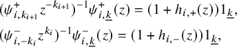 $$ \begin{align*} &(\psi^{+}_{i,k_{i+1}}z^{-k_{i+1}})^{-1} \psi^{+}_{i,\underline{k}}(z)=(1+h_{i,+}(z))1_{\underline{k}},\\ &(\psi^{-}_{i,-k_{i}}z^{k_{i}})^{-1} \psi^{-}_{i,\underline{k}}(z)=(1+h_{i,-}(z))1_{\underline{k}}, \end{align*} $$
where
 $h_{i,\pm }(z)=\sum _{r>0} h_{i,\pm r}z^{\mp r}$
.
$h_{i,\pm }(z)=\sum _{r>0} h_{i,\pm r}z^{\mp r}$
.
Remark A.3. From (A.10) and (A.11), it is easy to see that the action of
 $h_{i,\pm r}$
on the Grothendieck group
$h_{i,\pm r}$
on the Grothendieck group
 $K(\mathrm {Fl}_{\underline {k}}(\mathbb {C}^N))$
is given by
$K(\mathrm {Fl}_{\underline {k}}(\mathbb {C}^N))$
is given by
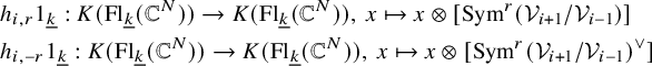 $$ \begin{align*} &h_{i,r}1_{\underline{k}}:K(\mathrm{Fl}_{\underline{k}}(\mathbb{C}^N)) \rightarrow K(\mathrm{Fl}_{\underline{k}}(\mathbb{C}^N)), \ x \mapsto x \otimes [\mathrm{Sym}^{r}(\mathcal{V}_{i+1}/\mathcal{V}_{i-1})] \\ &h_{i,-r}1_{\underline{k}}:K(\mathrm{Fl}_{\underline{k}}(\mathbb{C}^N)) \rightarrow K(\mathrm{Fl}_{\underline{k}}(\mathbb{C}^N)), \ x \mapsto x \otimes [\mathrm{Sym}^{r}(\mathcal{V}_{i+1}/\mathcal{V}_{i-1})^{\vee}] \end{align*} $$
where
 $r \geq 1$
.
$r \geq 1$
.
Then, we define inductively
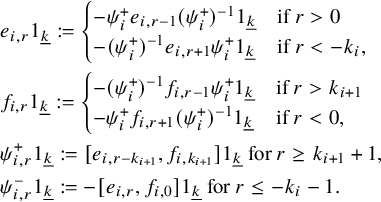 $$ \begin{align*} &e_{i,r}1_{\underline{k}}:= \begin{cases} -\psi^{+}_{i}e_{i,r-1}(\psi^{+}_{i})^{-1}1_{\underline{k}}& \text{if} \ r>0 \\ -(\psi^{+}_{i})^{-1}e_{i,r+1}\psi^{+}_{i}1_{\underline{k}}& \text{if} \ r<{-k_{i}},\\ \end{cases} \\ &f_{i,r}1_{\underline{k}}:= \begin{cases} -(\psi^{+}_{i})^{-1}f_{i,r-1}\psi^{+}_{i}1_{\underline{k}}& \text{if} \ r>{k_{i+1}} \\ -\psi^{+}_{i}f_{i,r+1}(\psi^{+}_{i})^{-1}1_{\underline{k}}& \text{if} \ r<0, \\ \end{cases}\\ &\psi^{+}_{i,r}1_{\underline{k}}:= [e_{i,{r-k_{i+1}}},f_{i,{k_{i+1}}}]1_{\underline{k}} \ \text{for} \ r \geq k_{i+1}+1, \\ &\psi^{-}_{i,r}1_{\underline{k}}:= -[e_{i,r},f_{i,0}]1_{\underline{k}} \ \text{for} \ r \leq -k_{i}-1. \end{align*} $$
We propose the following conjecture, which, roughly speaking, says that the two presentations defined by Definition A.1 and Definition 2.6 are equivalent.
Conjecture A.4. There is a
 $\mathbb {C}$
-algebra isomorphism
$\mathbb {C}$
-algebra isomorphism
 $\dot {\mathrm {\mathbf {U}}}_{0,N}(L\mathfrak {sl}_n) \rightarrow \dot {\mathrm {\mathbf {U}}}^{\prime }_{0,N}(L\mathfrak {sl}_n)$
such that
$\dot {\mathrm {\mathbf {U}}}_{0,N}(L\mathfrak {sl}_n) \rightarrow \dot {\mathrm {\mathbf {U}}}^{\prime }_{0,N}(L\mathfrak {sl}_n)$
such that
 $$\begin{align*}e_{i,r}1_{\underline{k}} \mapsto e_{i,r}1_{\underline{k}}, \ f_{i,r}1_{\underline{k}} \mapsto f_{i,r}1_{\underline{k}}, \ \psi^{+}_{i}1_{\underline{k}} \mapsto \psi^{+}_{i,k_{i+1}}1_{\underline{k}},\ \psi^{-}_{i}1_{\underline{k}} \mapsto \psi^{-}_{i,-k_{i}}1_{\underline{k}}, \end{align*}$$
for
 $1 \leq i \leq n-1$
.
$1 \leq i \leq n-1$
.
Acknowledgments
This article is the author’s thesis work, and the author would like to thank his supervisor Sabin Cautis for his patience and guidance. He provided many valuable ideas. Next, we want to thank Chun-Ju Lai, Harrison Chen, Hsueh-Yun Lin, Sz-Sheng Wang, and Wu-Yen Chuang for many helpful discussions. Finally, we thank Roman Bezrukavnikov, Joel Kamnitzer, Yukinobu Toda, Yu Zhao, and the anonymous referee for email correspondence and for providing some helpful comments about this article.
Competing interest
The author has no competing interests to declare.
Funding statement
The author was supported by the National Science and Technology Council grant 111-2628-M-001-007.


 Open access