


1 Introduction. Statement of main results
We consider the solid torus
 $$ \begin{align*}M=S^1 \times \mathbb{D},\quad \mathbb{D}=\{(y,z)\in\mathbb{R}^2:y^2+z^2<1\}, \end{align*} $$
where
 $S^1=\mathbb {R}/2\pi \mathbb {Z}$
.
$S^1=\mathbb {R}/2\pi \mathbb {Z}$
.
Consider a mapping
 $f:M\to M$
of class
$f:M\to M$
of class
 $C^{1+\varepsilon }$
, that is, with its differential being Hölder continuous, given by the formula
$C^{1+\varepsilon }$
, that is, with its differential being Hölder continuous, given by the formula
 $$ \begin{align} f(x,y,z)=(\eta(x), \unicode{x3bb}( x,y )+ u(x), \nu( x,y,z ) + v(x) ), \end{align} $$
with
 $\unicode{x3bb} (x,0)=\nu (x,0,0)=0$
. Assume that f has period
$\unicode{x3bb} (x,0)=\nu (x,0,0)=0$
. Assume that f has period
 $2\pi $
with respect to x so that it is well-defined on M. Assume that
$2\pi $
with respect to x so that it is well-defined on M. Assume that
 $\eta $
has degree
$\eta $
has degree
 $d>1$
.
$d>1$
.
Denote
 $\eta '={d\eta }/{dx}, \; \unicode{x3bb} '={d\unicode{x3bb} }/{dy}, \; \nu '={d\nu }/{dz}$
. Assume that
$\eta '={d\eta }/{dx}, \; \unicode{x3bb} '={d\unicode{x3bb} }/{dy}, \; \nu '={d\nu }/{dz}$
. Assume that
 $0<\nu ' < \unicode{x3bb} '<1$
and
$0<\nu ' < \unicode{x3bb} '<1$
and
 $1<\eta '<1/\unicode{x3bb} ' $
(some of these inequalities will be weakened later on to inequalities between Lyapunov exponents on
$1<\eta '<1/\unicode{x3bb} ' $
(some of these inequalities will be weakened later on to inequalities between Lyapunov exponents on
 $\Lambda $
, that is, integrals with respect to certain Gibbs measure). We could allow here
$\Lambda $
, that is, integrals with respect to certain Gibbs measure). We could allow here
 $-1<\unicode{x3bb} '<0$
(the same for
$-1<\unicode{x3bb} '<0$
(the same for
 $\nu '$
), but we assume it is positive to simplify the notation. We assume also that
$\nu '$
), but we assume it is positive to simplify the notation. We assume also that
 $f:M\to M$
is injective (using sometimes the name embedded).
$f:M\to M$
is injective (using sometimes the name embedded).
Such a solenoid in the linear case (or at least if
 $\eta '\equiv d$
) can be called a uniformly thin solenoid (for the definition of a thick linear solenoid, where
$\eta '\equiv d$
) can be called a uniformly thin solenoid (for the definition of a thick linear solenoid, where
 $\eta '\unicode{x3bb} '>1$
, see e.g. [Reference Rams15]). Compare the stronger uniform dissipation condition in §1.4.
$\eta '\unicode{x3bb} '>1$
, see e.g. [Reference Rams15]). Compare the stronger uniform dissipation condition in §1.4.
Then
 $$ \begin{align*}\Lambda:=\bigcap_{n=0}^\infty f^n(M) \end{align*} $$
is an invariant hyperbolic set, so called an expanding attractor. The assumption f is injective on M can be weakened to the assumption f is injective on
 $\Lambda $
, by replacing M with a solid torus being a sufficiently thin neighbourhood of
$\Lambda $
, by replacing M with a solid torus being a sufficiently thin neighbourhood of
 $\Lambda $
. However, for clarity, we assume the injectivity of f directly on M.
$\Lambda $
. However, for clarity, we assume the injectivity of f directly on M.
For each
 $p=(x,y,z)\in \Lambda $
, the disc
$p=(x,y,z)\in \Lambda $
, the disc
 $W^s_x=W^s(p)=\{(x',y',z'):x'=x\}$
is a (principal) component (in M) of the stable manifold of p and the interval
$W^s_x=W^s(p)=\{(x',y',z'):x'=x\}$
is a (principal) component (in M) of the stable manifold of p and the interval
 $W^{ss}_{x,y}=W^{ss}(p)=\{(x',y',z'):x'=x, y'=y\}$
is a (principal) component of strong stable manifold of p. Unstable manifolds
$W^{ss}_{x,y}=W^{ss}(p)=\{(x',y',z'):x'=x, y'=y\}$
is a (principal) component of strong stable manifold of p. Unstable manifolds
 $W^u(p)$
are more complicated, each is dense in
$W^u(p)$
are more complicated, each is dense in
 $\Lambda $
and for each
$\Lambda $
and for each
 $x,x'\in \mathbb {R}^1$
, the unstable lamination of
$x,x'\in \mathbb {R}^1$
, the unstable lamination of
 $\Lambda $
defines the holonomy map
$\Lambda $
defines the holonomy map
 $h_{x,x'}:W^s_{x/2\pi \mathbb {Z}}\cap \Lambda \to W^s_{x'/2\pi \mathbb {Z}}\cap \Lambda $
.
$h_{x,x'}:W^s_{x/2\pi \mathbb {Z}}\cap \Lambda \to W^s_{x'/2\pi \mathbb {Z}}\cap \Lambda $
.
Sometimes we write
 $W^s_x$
in place of
$W^s_x$
in place of
 $W^s_{x/2\pi \mathbb {Z}}$
. Denote by
$W^s_{x/2\pi \mathbb {Z}}$
. Denote by
 $\pi _x$
the projection
$\pi _x$
the projection
 $(x,y,z)\mapsto x$
. The part of global
$(x,y,z)\mapsto x$
. The part of global
 $W^u(p)$
, which is the lift of
$W^u(p)$
, which is the lift of
 $[x,x']\subset \mathbb {R}$
for
$[x,x']\subset \mathbb {R}$
for
 $\pi _x$
, will be denoted
$\pi _x$
, will be denoted
 $W^u_{[x,x']}(p)$
. For
$W^u_{[x,x']}(p)$
. For
 $[x,x']$
equal to
$[x,x']$
equal to
 $[0,2\pi ]$
or slightly bigger, clear from the context, we shall sometimes just write
$[0,2\pi ]$
or slightly bigger, clear from the context, we shall sometimes just write
 $W^u(p)$
.
$W^u(p)$
.
Denote by
 $\pi _{x,y}$
the projection
$\pi _{x,y}$
the projection
 $(x,y,z) \mapsto (x,y)$
. We assume in this paper the following transversality assumption: each intersection of two distinct
$(x,y,z) \mapsto (x,y)$
. We assume in this paper the following transversality assumption: each intersection of two distinct
 $\pi _{x,y}(W^u(p))$
and
$\pi _{x,y}(W^u(p))$
and
 $\pi _{x,y}(W^u(q))$
is transversal.
$\pi _{x,y}(W^u(q))$
is transversal.
Let
 $\mu =\mu _{t_0}$
be the Gibbs measure (equilibrium state) on
$\mu =\mu _{t_0}$
be the Gibbs measure (equilibrium state) on
 $\Lambda $
for the potential
$\Lambda $
for the potential
 $t_0\log |\unicode{x3bb} '|$
, where
$t_0\log |\unicode{x3bb} '|$
, where
 $t=t_0$
is zero of the topological pressure
$t=t_0$
is zero of the topological pressure
 $t\mapsto P(f,t\log \unicode{x3bb} ')$
. The measure
$t\mapsto P(f,t\log \unicode{x3bb} ')$
. The measure
 $\mu $
can be called geometric or SRB in the stable direction or just stable SRB-measure. Denote by
$\mu $
can be called geometric or SRB in the stable direction or just stable SRB-measure. Denote by
 $\mu ^s_x$
its conditional measures on
$\mu ^s_x$
its conditional measures on
 $W^s_x$
for each x, see explanations following Lemma 3.6.
$W^s_x$
for each x, see explanations following Lemma 3.6.
Definition 1.1. (Thin solenoid)
The solenoid
 $\Lambda $
for injective
$\Lambda $
for injective
 $f:M\to M$
as in equation (1.1) satisfying
$f:M\to M$
as in equation (1.1) satisfying
 $\chi _{\mu }(\nu ')<\chi _{\mu } (\unicode{x3bb} ')< -\chi _{\mu }(\eta ')$
for
$\chi _{\mu }(\nu ')<\chi _{\mu } (\unicode{x3bb} ')< -\chi _{\mu }(\eta ')$
for
 $\mu $
being the stable SRB-measure on
$\mu $
being the stable SRB-measure on
 $\Lambda $
, for Lyapunov exponents
$\Lambda $
, for Lyapunov exponents
 $\chi _{\mu }(\xi ):=\int \log \xi \, d\mu $
for
$\chi _{\mu }(\xi ):=\int \log \xi \, d\mu $
for
 $\xi =\nu ',\unicode{x3bb} '$
and
$\xi =\nu ',\unicode{x3bb} '$
and
 $\eta '$
, respectively, is called a non-uniformly thin, or just thin, solenoid.
$\eta '$
, respectively, is called a non-uniformly thin, or just thin, solenoid.
We prove the following theorems.
Theorem 1.2. Let
 $\Lambda $
be a non-uniformly thin solenoid for
$\Lambda $
be a non-uniformly thin solenoid for
 $f:M\to M$
as in the definition above, which satisfies the transversality assumption. Then, for
$f:M\to M$
as in the definition above, which satisfies the transversality assumption. Then, for
 $\operatorname {\mathrm {HD}}$
denoting Hausdorff dimension and for every
$\operatorname {\mathrm {HD}}$
denoting Hausdorff dimension and for every
 $x\in S^1$
:
$x\in S^1$
:
-
(1)
 $\operatorname {\mathrm {HD}}(\Lambda \cap W^s_x)=t_0$
;
$\operatorname {\mathrm {HD}}(\Lambda \cap W^s_x)=t_0$
; -
(2)
$\operatorname {\mathrm {HD}}(\Lambda )=1+t_0$
.

Theorem 1.3. Under the assumptions of Theorem 1.2, for
 $\Pi _t$
denoting packing measure in dimension t, for every
$\Pi _t$
denoting packing measure in dimension t, for every
 $x\in S^1$
, it holds
$x\in S^1$
, it holds
 $0<\Pi _{t_0}(\Lambda \cap W^s_x)<\infty $
. Moreover,
$0<\Pi _{t_0}(\Lambda \cap W^s_x)<\infty $
. Moreover,
 $ 0<\Pi _{1+t_0}(\Lambda )<\infty $
.
$ 0<\Pi _{1+t_0}(\Lambda )<\infty $
.
Theorem 1.4. Under the assumptions of Theorem 1.2, for
 $\mathrm {HM}_t$
denoting Hausdorff measure in dimension t,
$\mathrm {HM}_t$
denoting Hausdorff measure in dimension t,
 $\mathrm {HM}_{t_0}(\Lambda \cap W^s_x)=0$
for every
$\mathrm {HM}_{t_0}(\Lambda \cap W^s_x)=0$
for every
 $x\in S^1$
. Moreover,
$x\in S^1$
. Moreover,
 $\mathrm {HM}_{1+t_0}(\Lambda ) =0$
.
$\mathrm {HM}_{1+t_0}(\Lambda ) =0$
.
Now we need the following definition.
Definition 1.5. (Bunching condition)
We say that our thin solenoid
 $\Lambda $
satisfies the bunching condition if
$\Lambda $
satisfies the bunching condition if
 $\eta '(x)> \unicode{x3bb} '(x)/\nu '(x)$
for every
$\eta '(x)> \unicode{x3bb} '(x)/\nu '(x)$
for every
 $x\in \Lambda $
.
$x\in \Lambda $
.
A theorem used in particular to compare sizes of
 $\Lambda \cap W^s_x$
for varying x, is the following.
$\Lambda \cap W^s_x$
for varying x, is the following.
Theorem 1.6. Under the assumptions of Theorem 1.2, if the bunching condition is satisfied, then all the holonomies
 $h_{x,x'}$
for
$h_{x,x'}$
for
 $x,x'\in \mathbb {R}$
are uniformly Lipschitz continuous.
$x,x'\in \mathbb {R}$
are uniformly Lipschitz continuous.
If the bunching condition is not assumed, then for each R, there exists
 $\operatorname {\mathrm {Lip}}(R)>0$
such that for each x, there is a set
$\operatorname {\mathrm {Lip}}(R)>0$
such that for each x, there is a set
 $L_x\subset W^s_x\cap \Lambda $
such that for all
$L_x\subset W^s_x\cap \Lambda $
such that for all
 $x'$
satisfying
$x'$
satisfying
 $|x-x'|<R$
, the holonomies
$|x-x'|<R$
, the holonomies
 $h_{x,x'}$
are locally bi-Lipschitz continuous with a common constant
$h_{x,x'}$
are locally bi-Lipschitz continuous with a common constant
 $\operatorname {\mathrm {Lip}}(R)$
and
$\operatorname {\mathrm {Lip}}(R)$
and
 $\mu ^s_x(\Lambda \cap W^s_x \setminus L_x)= 0$
.
$\mu ^s_x(\Lambda \cap W^s_x \setminus L_x)= 0$
.
In fact,
 $\mu ^s_x(NL^w \cap W^s_x)=0$
for a certain weak non-Lipschitz set
$\mu ^s_x(NL^w \cap W^s_x)=0$
for a certain weak non-Lipschitz set
 $NL^w$
invariant under all
$NL^w$
invariant under all
 $h_{x,x'}$
for
$h_{x,x'}$
for
 $0\le x,x'\le 2\pi $
, which, intersected with
$0\le x,x'\le 2\pi $
, which, intersected with
 $W_x^s$
, is bigger than the complement of Lipschitz
$W_x^s$
, is bigger than the complement of Lipschitz
 $L_x$
. Moreover,
$L_x$
. Moreover,
 $\operatorname {\mathrm {HD}} (NL^w \cap W^s_x) < t_0$
.
$\operatorname {\mathrm {HD}} (NL^w \cap W^s_x) < t_0$
.
Here ‘local’ means for every
 $p\in L_x$
, there exists
$p\in L_x$
, there exists
 $\delta $
such that for all
$\delta $
such that for all
 $q\in W^s_x\cap \Lambda \cap B(p,\delta )$
and
$q\in W^s_x\cap \Lambda \cap B(p,\delta )$
and
 $|x'-x|<R$
, the Lipschitz condition with the constant
$|x'-x|<R$
, the Lipschitz condition with the constant
 $\operatorname {\mathrm {Lip}}(R)$
holds for
$\operatorname {\mathrm {Lip}}(R)$
holds for
 $h_{x,x'}$
.
$h_{x,x'}$
.
The bunching condition above appeared in a related setting in [Reference Pugh, Shub and Wilkinson13], see also [Reference Crovisier and Potrie6, Theorem 4.21] for a stronger conclusion that the unstable foliation is
 $C^1$
.
$C^1$
.
Some of the assertions above hold also for the projections to the
 $\{(x,y)\}$
plane, in particular the following.
$\{(x,y)\}$
plane, in particular the following.
Theorem 1.7. Under the assumptions of Theorem 1.2,
 $\operatorname {\mathrm {HD}}(\pi _{x,y}(\Lambda \cap W^s_x))=t_0$
and
$\operatorname {\mathrm {HD}}(\pi _{x,y}(\Lambda \cap W^s_x))=t_0$
and
 $\operatorname {\mathrm {HD}}(\pi _{x,y}(\Lambda ))=1+t_0$
.
$\operatorname {\mathrm {HD}}(\pi _{x,y}(\Lambda ))=1+t_0$
.
We do not know if
 $0<\Pi _{t_0}(\pi _{x,y}(\Lambda \cap W^s_x))<\infty $
or
$0<\Pi _{t_0}(\pi _{x,y}(\Lambda \cap W^s_x))<\infty $
or
 $ 0<\Pi _{1+t_0}(\pi _{x,y}(\Lambda ))<\infty $
.
$ 0<\Pi _{1+t_0}(\pi _{x,y}(\Lambda ))<\infty $
.
The assertions of Theorem 1.2 almost automatically hold for Hausdorff dimension replaced by the upper box dimension
 $\overline {\operatorname {\mathrm {BD}}}$
. Indeed, the estimates from below follow from
$\overline {\operatorname {\mathrm {BD}}}$
. Indeed, the estimates from below follow from
 $\operatorname {\mathrm {HD}}\le \overline {\operatorname {\mathrm {BD}}}$
. The estimate
$\operatorname {\mathrm {HD}}\le \overline {\operatorname {\mathrm {BD}}}$
. The estimate
 $\overline {\operatorname {\mathrm {BD}}}(\Lambda \cap W^s_x)\le t_0$
follows from Lemma 4.3. The estimate
$\overline {\operatorname {\mathrm {BD}}}(\Lambda \cap W^s_x)\le t_0$
follows from Lemma 4.3. The estimate
 $\overline {\operatorname {\mathrm {BD}}}(\Lambda )\le 1+ t_0$
follows from the proof of Theorem 4.2, Step 3.
$\overline {\operatorname {\mathrm {BD}}}(\Lambda )\le 1+ t_0$
follows from the proof of Theorem 4.2, Step 3.
1.1 On the linear case
The mapping f in equation (1.1) is called lower triangular (because such is the differential
 $Df$
in the
$Df$
in the
 $y,z$
direction) nonlinear. Our paper complements the study of the linear diagonal case
$y,z$
direction) nonlinear. Our paper complements the study of the linear diagonal case
 $$ \begin{align} f(x,y,z)=(dx(\mathrm{mod}\ 2\pi), \unicode{x3bb} y + u(x), \nu z + v(x) ), \end{align} $$
with
 $0<\nu <\unicode{x3bb} < 1/d$
. It was done by Hasselblatt and Schmeling in [Reference Hasselblatt, Schmeling, Hasselblatt, Brin and Pesin9], where, nevertheless, there were hints concerning the nonlinear situations, and by Rams and Simon [Reference Rams and Simon17]. Namely, Theorems 1.2,1.3, and 1.4 generalize [Reference Hasselblatt, Schmeling, Hasselblatt, Brin and Pesin9] and Theorem 1.4 generalizes [Reference Rams and Simon17]. It should be noted that Theorem 1.3 was proved in [Reference Rams and Simon17] only for Lebesgue almost every (a.e.) x.
$0<\nu <\unicode{x3bb} < 1/d$
. It was done by Hasselblatt and Schmeling in [Reference Hasselblatt, Schmeling, Hasselblatt, Brin and Pesin9], where, nevertheless, there were hints concerning the nonlinear situations, and by Rams and Simon [Reference Rams and Simon17]. Namely, Theorems 1.2,1.3, and 1.4 generalize [Reference Hasselblatt, Schmeling, Hasselblatt, Brin and Pesin9] and Theorem 1.4 generalizes [Reference Rams and Simon17]. It should be noted that Theorem 1.3 was proved in [Reference Rams and Simon17] only for Lebesgue almost every (a.e.) x.
1.2 Transversally conformal case
This is the case where f is conformal on every
 $W^s$
well understood. Theorems 1.2 and 1.3 hold, though the dimension
$W^s$
well understood. Theorems 1.2 and 1.3 hold, though the dimension
 $t_0$
can be larger than one (in a thick case). Packing and Hausdorff measures on
$t_0$
can be larger than one (in a thick case). Packing and Hausdorff measures on
 $W^s$
in dimension
$W^s$
in dimension
 $t_0$
are equivalent. In fact, this is a transversally complex one-dimensional (1D) situation, whereas our non-conformal case corresponds after
$t_0$
are equivalent. In fact, this is a transversally complex one-dimensional (1D) situation, whereas our non-conformal case corresponds after
 $\pi _{x,y}$
-projection to a transversally real 1D situation with overlaps.
$\pi _{x,y}$
-projection to a transversally real 1D situation with overlaps.
1.3 Motivation
Let us present a geometric picture of the solenoid. It helps to think not of the solenoid itself (which is locally just a Cantor bouquet of almost parallel lines and is hard to analyse with an untrained eye) but of its approximations
 $f^n(M)$
. Each of the approximations is a tube, winding around along
$f^n(M)$
. Each of the approximations is a tube, winding around along
 $S^1$
and going around
$S^1$
and going around
 $d^n$
times. Thus, every section of
$d^n$
times. Thus, every section of
 $f^n(M)$
with a disc
$f^n(M)$
with a disc
 $W_x^s=\{x\}\times \mathbb D$
is a disjoint union of
$W_x^s=\{x\}\times \mathbb D$
is a disjoint union of
 $d^n$
components, where each disc is a (slightly deformed) ellipse with exponentially increasing ratio of the large semiaxis to the small semiaxis, and all the large semiaxes pointing roughly in the same
$d^n$
components, where each disc is a (slightly deformed) ellipse with exponentially increasing ratio of the large semiaxis to the small semiaxis, and all the large semiaxes pointing roughly in the same
 $\{y\}$
direction. See Figure 1. As already mentioned, the approximate ellipses are disjoint, but there are plenty of sections in which some of the ellipses are very close to each other, in a distance exponentially smaller than their diameters. One of the main concerns in our study will be the understanding of the way those ellipses ‘move’ as we move the section plane around
$\{y\}$
direction. See Figure 1. As already mentioned, the approximate ellipses are disjoint, but there are plenty of sections in which some of the ellipses are very close to each other, in a distance exponentially smaller than their diameters. One of the main concerns in our study will be the understanding of the way those ellipses ‘move’ as we move the section plane around
 $S^1$
.
$S^1$
.

Figure 1 Geometric picture of the solenoid.
This picture closely resembles the picture of an affine iterated function system, or maybe even better: the averaged picture of many different but similar affine iterated function systems (as each ellipse in the section comes with a different backward path, and is thus produced by a different collection of non-conformal contracting maps). An important element of the picture is that the contracting maps in the sections satisfy a version of the domination property, that is, the strong contracting direction in one iteration stays close to the strong contracting direction in the following iterations. That is, we clearly have two different negative Lyapunov exponents in our system.
This picture lets us expect a behaviour similar to the known generic behaviour of affine iterated function systems. We expect the Hausdorff and packing and box dimensions of each section to be given by Falconer’s singular value pressure formula, which, in our ‘thin’ case, should depend only on what happens in the expanding and weakly contracting directions (in particular, the dimensions should be preserved by the projection to the
 $\{(x,y)\}$
plane). Moreover, like in simpler solenoid cases, we expect that the situations when two ellipses pass nearby (which are unavoidable owing to the very geometry of the solenoid) should have an effect strong enough to zero the Hausdorff measure, but the packing measure should stay positive and finite. Those are exactly the statements we eventually prove in Theorems 1.2–1.4 and 1.7.
$\{(x,y)\}$
plane). Moreover, like in simpler solenoid cases, we expect that the situations when two ellipses pass nearby (which are unavoidable owing to the very geometry of the solenoid) should have an effect strong enough to zero the Hausdorff measure, but the packing measure should stay positive and finite. Those are exactly the statements we eventually prove in Theorems 1.2–1.4 and 1.7.
Hasselblatt and Schmeling stated in [Reference Hasselblatt, Schmeling, Hasselblatt, Brin and Pesin9] (see some history and other references there, in particular [Reference Bothe3]) the following.
Conjecture 1.8. The fractal dimension of a hyperbolic set is the sum of those of its stable and unstable slices, where ‘fractal’ can mean either Hausdorff or upper box dimension.
For solenoids, in [Reference Hasselblatt, Schmeling, Hasselblatt, Brin and Pesin9] and here, an affirmative answer on Hausdorff dimension has been proven. Hausdorff dimension in the stable direction is
 $t_0$
and in unstable 1, that is,
$t_0$
and in unstable 1, that is,
 $1+t_0$
together. Notice that this is dimension
$1+t_0$
together. Notice that this is dimension
 $t_0$
of conditional measures of
$t_0$
of conditional measures of
 $\mu $
geometric (SRB) in the stable direction (see above) and of dimension 1 of an SRB measure in the unstable direction. Both SRB measures are usually different (even mutually singular), unless (e.g.) in the diagonal linear case, where both measures coincide with the measure of maximal entropy.
$\mu $
geometric (SRB) in the stable direction (see above) and of dimension 1 of an SRB measure in the unstable direction. Both SRB measures are usually different (even mutually singular), unless (e.g.) in the diagonal linear case, where both measures coincide with the measure of maximal entropy.
For any invariant hyperbolic measure
 $\nu $
, indeed
$\nu $
, indeed
 $\operatorname {\mathrm {HD}}(\nu )=\operatorname {\mathrm {HD}}(\nu ^s)+\operatorname {\mathrm {HD}}(\nu ^u)$
, see [Reference Barreira, Pesin and Schmeling1], but even supremum of
$\operatorname {\mathrm {HD}}(\nu )=\operatorname {\mathrm {HD}}(\nu ^s)+\operatorname {\mathrm {HD}}(\nu ^u)$
, see [Reference Barreira, Pesin and Schmeling1], but even supremum of
 $\operatorname {\mathrm {HD}}(\nu )$
over invariant
$\operatorname {\mathrm {HD}}(\nu )$
over invariant
 $\nu $
on
$\nu $
on
 $\Lambda $
can be less than
$\Lambda $
can be less than
 $\operatorname {\mathrm {HD}}(\Lambda )$
. See e.g. [Reference Rams16]. So in a general case, one is forced to use both the SRB measures.
$\operatorname {\mathrm {HD}}(\Lambda )$
. See e.g. [Reference Rams16]. So in a general case, one is forced to use both the SRB measures.
Finally note that Hasselblatt and Schmeling relax the assumption of transversality to the assumption that the intersections of
 $\pi _{x,y}$
projections of
$\pi _{x,y}$
projections of
 $W^u$
are non-flat. This in particular holds for all real analytic (that is, with the functions
$W^u$
are non-flat. This in particular holds for all real analytic (that is, with the functions
 $u,v$
real analytic) linear solenoids, see [Reference Hasselblatt, Schmeling, Hasselblatt, Brin and Pesin9]. A natural challenge would be to generalize our nonlinear theory to a general real-analytic (non-transversal) case.
$u,v$
real analytic) linear solenoids, see [Reference Hasselblatt, Schmeling, Hasselblatt, Brin and Pesin9]. A natural challenge would be to generalize our nonlinear theory to a general real-analytic (non-transversal) case.
1.4 Outline
In §3, we prove a part of Theorem 1.6 saying that the points in
 $W^s_x$
, where a holonomy
$W^s_x$
, where a holonomy
 $h_{x,x'}$
is not locally bi-Lipschitz, have measure
$h_{x,x'}$
is not locally bi-Lipschitz, have measure
 $\mu $
equal 0. This follows (and clarifies) [Reference Hasselblatt, Schmeling, Hasselblatt, Brin and Pesin9]. In fact, we prove that a bigger set has measure 0, the set of p which are not strong Lipschitz, called above weak non-Lipschitz. For such a p, the projection
$\mu $
equal 0. This follows (and clarifies) [Reference Hasselblatt, Schmeling, Hasselblatt, Brin and Pesin9]. In fact, we prove that a bigger set has measure 0, the set of p which are not strong Lipschitz, called above weak non-Lipschitz. For such a p, the projection
 $\pi _{x,y}(W^u(p))$
intersects some
$\pi _{x,y}(W^u(p))$
intersects some
 $\pi _{x,y}(W^u(q))$
values for
$\pi _{x,y}(W^u(q))$
values for
 $q\notin W^u(p)$
arbitrarily close to
$q\notin W^u(p)$
arbitrarily close to
 $W^u(p)$
. Equivalently, p is strong Lipschitz if
$W^u(p)$
. Equivalently, p is strong Lipschitz if
 $W^{ss}_{\mathrm {loc}}(p)=\{p\}$
, so counting Hausdorff dimension only
$W^{ss}_{\mathrm {loc}}(p)=\{p\}$
, so counting Hausdorff dimension only
 $E^s/E^{ss}$
counts, so
$E^s/E^{ss}$
counts, so
 $\operatorname {\mathrm {HD}}(\Lambda \cap W^s)=h_\mu (f)/-\chi _\mu (\unicode{x3bb} ') = t_0$
, where
$\operatorname {\mathrm {HD}}(\Lambda \cap W^s)=h_\mu (f)/-\chi _\mu (\unicode{x3bb} ') = t_0$
, where
 $h_\mu (f)$
is the measure (Kolmogorov’s) entropy, [Reference Ledrappier and Young10]. This is done in §4, and yields Theorem 1.2. Again we roughly follow [Reference Hasselblatt, Schmeling, Hasselblatt, Brin and Pesin9].
$h_\mu (f)$
is the measure (Kolmogorov’s) entropy, [Reference Ledrappier and Young10]. This is done in §4, and yields Theorem 1.2. Again we roughly follow [Reference Hasselblatt, Schmeling, Hasselblatt, Brin and Pesin9].
In §3, Theorem 1.6 is in fact proved under the assumption stronger than
 $ \chi _\mu (\unicode{x3bb} ')< - \chi _\mu (\eta ') $
, namely under the assumption
$ \chi _\mu (\unicode{x3bb} ')< - \chi _\mu (\eta ') $
, namely under the assumption
 $\sup \unicode{x3bb} '<1/\sup \eta '$
, called uniform dissipation.
$\sup \unicode{x3bb} '<1/\sup \eta '$
, called uniform dissipation.
Note that Lipschitz property is related to Theorem 1.2 on Hausdorff dimension a little bit by chance, saying however that
 $\operatorname {\mathrm {HD}}(W^s_x\cap \Lambda )$
does not depend on x. In fact, holonomy being Lipschitz is a weak condition, e.g. it holds for all holonomies
$\operatorname {\mathrm {HD}}(W^s_x\cap \Lambda )$
does not depend on x. In fact, holonomy being Lipschitz is a weak condition, e.g. it holds for all holonomies
 $h_{x,x'}$
provided
$h_{x,x'}$
provided
 $\eta '>\unicode{x3bb} '/\nu '$
, as in Theorem 1.6 (well known), as a twisting, hurting Lipschitz property cannot develop if
$\eta '>\unicode{x3bb} '/\nu '$
, as in Theorem 1.6 (well known), as a twisting, hurting Lipschitz property cannot develop if
 $f^{-n}$
squeezes (by
$f^{-n}$
squeezes (by
 $(\eta ')^{-1}$
) too much. The Lipschitz property is crucial to conclude
$(\eta ')^{-1}$
) too much. The Lipschitz property is crucial to conclude
 $\operatorname {\mathrm {HD}}(W^s_x\cap \Lambda )=t_0 \Rightarrow \operatorname {\mathrm {HD}}(\Lambda )=1+t_0$
in Theorem 1.2. Compare Conjecture 1.8 above.
$\operatorname {\mathrm {HD}}(W^s_x\cap \Lambda )=t_0 \Rightarrow \operatorname {\mathrm {HD}}(\Lambda )=1+t_0$
in Theorem 1.2. Compare Conjecture 1.8 above.
Theorem 1.3 is proved in §5. The proof has common points with [Reference Rams and Simon17]. Analysis is more delicate than in the proof of Theorem 1.2. We prove that for
 $\mu $
-a.e. p for a sequence of n values, the
$\mu $
-a.e. p for a sequence of n values, the
 $\pi _{x,y}$
-projection of the tube
$\pi _{x,y}$
-projection of the tube
 $f^n(M)$
(truncated to
$f^n(M)$
(truncated to
 $[0,2\pi ]$
), called of order n containing p, intersects only a bounded number of other projections of tubes of order n.
$[0,2\pi ]$
), called of order n containing p, intersects only a bounded number of other projections of tubes of order n.
Theorem 1.4 is proved in §6, again using an idea from [Reference Rams and Simon17]. It uses the fact of arbitrarily high multiplicity of overlapping of projections of tubes of order n for
 $\mu $
-a.e. p.
$\mu $
-a.e. p.
The estimate
 $\operatorname {\mathrm {HD}}(NL^w_x)<t_0$
in Theorem 1.6 is proved in §7, together with a more precise estimate, following from a large deviations estimate concerning Birkhoff averages.
$\operatorname {\mathrm {HD}}(NL^w_x)<t_0$
in Theorem 1.6 is proved in §7, together with a more precise estimate, following from a large deviations estimate concerning Birkhoff averages.
Theorem 1.7 follows from other theorems because the assertions on dimensions are verified on the sets where the projection
 $\pi _{x,y}$
is finite-to-one.
$\pi _{x,y}$
is finite-to-one.
Section 7 also contains a remark on general Williams 1D expanding attractors and a remark on a possibility of integrating general solenoids to triangular as in equation (1.1).
2 Holonomy along unstable lamination
Definition 2.1. We will now introduce a symbolic description on the attractor, defining an ‘almost bijection’
 $\rho : \Sigma _d \to \Lambda $
, where
$\rho : \Sigma _d \to \Lambda $
, where
 $\Sigma _d = \{0,1,\ldots , d-1\}^{\mathbb {Z}}$
is the usual two-sided full-shift space on d symbols. Why it is only an ‘almost bijection’ will be explained soon. Moreover, it will be done in such a way that
$\Sigma _d = \{0,1,\ldots , d-1\}^{\mathbb {Z}}$
is the usual two-sided full-shift space on d symbols. Why it is only an ‘almost bijection’ will be explained soon. Moreover, it will be done in such a way that
 $\rho $
semi-conjugates the left shift
$\rho $
semi-conjugates the left shift
 $\varsigma $
acting on
$\varsigma $
acting on
 $\Sigma _d$
to
$\Sigma _d$
to
 $f|_\Lambda $
, namely
$f|_\Lambda $
, namely
 $\rho \circ \varsigma = f \circ \rho $
. Denote else the elements of
$\rho \circ \varsigma = f \circ \rho $
. Denote else the elements of
 $\Sigma _d$
by
$\Sigma _d$
by
 $\underline {i}=(\ldots , i_{-n}, \ldots , i_0| i_1, \ldots , i_n, \ldots )$
, where the vertical line separates entries with non-positive indices from the entries with positive indices.
$\underline {i}=(\ldots , i_{-n}, \ldots , i_0| i_1, \ldots , i_n, \ldots )$
, where the vertical line separates entries with non-positive indices from the entries with positive indices.
Let us start with closer explanations from the x coordinate. Looking at equation (1.1), we see that if
 $(x',y',z')=f(x,y,z)$
, then
$(x',y',z')=f(x,y,z)$
, then
 $x'$
does depend only on x, not on y or z. The restriction of f to the first coordinate is the d-to-1 expanding map
$x'$
does depend only on x, not on y or z. The restriction of f to the first coordinate is the d-to-1 expanding map
 $\eta $
. Denote by
$\eta $
. Denote by
 $a_0,\ldots ,a_{d-1},a_d=a_0$
the points of
$a_0,\ldots ,a_{d-1},a_d=a_0$
the points of
 $\eta ^{-1}(0)\in \mathbb {R}/2\pi \mathbb {Z}=S^1$
numbered in increasing order. We can assume that
$\eta ^{-1}(0)\in \mathbb {R}/2\pi \mathbb {Z}=S^1$
numbered in increasing order. We can assume that
 $a_0=0=\eta (0)$
. For
$a_0=0=\eta (0)$
. For
 $i=0,1,\ldots , d-1$
, we denote
$i=0,1,\ldots , d-1$
, we denote
 $V_{|i}:=[a_i, a_{i+1}]\times \mathbb D$
; those sets will be called vertical cylinders of level 1. We can then define for every
$V_{|i}:=[a_i, a_{i+1}]\times \mathbb D$
; those sets will be called vertical cylinders of level 1. We can then define for every
 $n=1,2, \ldots $
the vertical cylinders of level n, by
$n=1,2, \ldots $
the vertical cylinders of level n, by
 $$ \begin{align*}V_{i_1,\ldots,i_n}=\{p=(x,y,z)\in M:\ f^{k-1}(p)\in V_{|i_k} \text{ for}\ k=1,\ldots,n\}. \end{align*} $$
For every sequence
 $(i_1, i_2,\ldots )\in \{0,\ldots , d-1\}^{\mathbb {N}}$
, there exists exactly one
$(i_1, i_2,\ldots )\in \{0,\ldots , d-1\}^{\mathbb {N}}$
, there exists exactly one
 $x\in S^1$
, such that
$x\in S^1$
, such that
 $$ \begin{align} \bigcap_{n=1}^\infty V_{|i_1,\ldots,i_n} = \{x\} \times \mathbb D, \end{align} $$
and vice versa: for all except countably many points
 $x\in S^1$
, there exists exactly one sequence
$x\in S^1$
, there exists exactly one sequence
 $(i_1, i_2,\ldots )\in \{0,\ldots , d-1\}^{\mathbb {N}}$
such that equation (2.1) holds. The exceptions are the points x such that
$(i_1, i_2,\ldots )\in \{0,\ldots , d-1\}^{\mathbb {N}}$
such that equation (2.1) holds. The exceptions are the points x such that
 $\eta ^k(x)=0$
for some
$\eta ^k(x)=0$
for some
 $k\in \mathbb {N}$
. For each of those points, one can find exactly two sequences satisfying equation (2.1). We note that
$k\in \mathbb {N}$
. For each of those points, one can find exactly two sequences satisfying equation (2.1). We note that
 $f^{k-1}(p)\in V_{|i_k}$
is equivalent to
$f^{k-1}(p)\in V_{|i_k}$
is equivalent to
 $\eta ^{k-1}(x)\in [a_{i_k},a_{i_k+1}]$
, so what we described up to this point is the usual construction of a symbolic description for an expanding map of the circle.
$\eta ^{k-1}(x)\in [a_{i_k},a_{i_k+1}]$
, so what we described up to this point is the usual construction of a symbolic description for an expanding map of the circle.
Let us now define the horizontal cylinders of level
 $n=0,1,2, \ldots $
by
$n=0,1,2, \ldots $
by
 $$\begin{align*}H_{i_{-n},\ldots, i_0|} := f^{n+1}(V_{|i_{-n},\ldots, i_0}), \end{align*}$$
and then define
 $$\begin{align*}\rho(\underline{i}):= \lim_{n\to\infty} V_{|i_1,\ldots, i_n} \cap H_{i_{-n},\ldots, i_0|}. \end{align*}$$
The fact that
 $\rho $
semi-conjugates
$\rho $
semi-conjugates
 $\varsigma $
to
$\varsigma $
to
 $f|_\Lambda $
is clear from the definitions.
$f|_\Lambda $
is clear from the definitions.
We will denote by
 $V(n)$
and
$V(n)$
and
 $H(n)$
the sets of all vertical (respectively horizontal) cylinders of level n. For a given
$H(n)$
the sets of all vertical (respectively horizontal) cylinders of level n. For a given
 $p\in \Lambda $
, we will denote by
$p\in \Lambda $
, we will denote by
 $V_n(p)$
and
$V_n(p)$
and
 $H_n(p)$
the vertical and horizontal cylinder of n, containing p. Sometimes we will just write
$H_n(p)$
the vertical and horizontal cylinder of n, containing p. Sometimes we will just write
 $H_n$
and
$H_n$
and
 $V_n$
if we do not specify p.
$V_n$
if we do not specify p.
We note that
 $\rho (\underline {i})=(x,y,z)$
, with x depending on
$\rho (\underline {i})=(x,y,z)$
, with x depending on
 $i_1, i_2, \ldots $
and
$i_1, i_2, \ldots $
and
 $(y,z)$
depending on x and on
$(y,z)$
depending on x and on
 $i_0,i_{-1},\ldots $
. It makes sense to write
$i_0,i_{-1},\ldots $
. It makes sense to write
 $\Sigma _d = \Sigma _d^- \times \Sigma _d^+$
with
$\Sigma _d = \Sigma _d^- \times \Sigma _d^+$
with
 $\Sigma _d^-, \Sigma _d^+$
denoting the one-sided shift spaces on d symbols, the former given by non-positive entries and the latter by the positive entries. We then denote
$\Sigma _d^-, \Sigma _d^+$
denoting the one-sided shift spaces on d symbols, the former given by non-positive entries and the latter by the positive entries. We then denote
 $$\begin{align*}W^u(\underline{i}) = \bigcap_{n=0}^\infty H_{i_{-n},\ldots, i_0|},\ \ \ W^s(\underline{i}) = \bigcap_{n=1}^\infty V_{|i_1,\ldots, i_n}. \end{align*}$$
Clearly,
 $\rho (\underline {i}) = W^u(\underline {i}) \cap W^s(\underline {i})$
. We will also use the notation
$\rho (\underline {i}) = W^u(\underline {i}) \cap W^s(\underline {i})$
. We will also use the notation
 $W^u(p), W^s(p)$
for
$W^u(p), W^s(p)$
for
 $p\in \Lambda $
, as the shortcut for
$p\in \Lambda $
, as the shortcut for
 $W^u(\rho ^{-1}(p)), W^s(\rho ^{-1}(p))$
. We note that as
$W^u(\rho ^{-1}(p)), W^s(\rho ^{-1}(p))$
. We note that as
 $\eta $
is expanding and
$\eta $
is expanding and
 $\unicode{x3bb} , \nu $
are contracting,
$\unicode{x3bb} , \nu $
are contracting,
 $W^u(p)$
and
$W^u(p)$
and
 $W^s(p)$
are pieces of the unstable and stable manifolds at
$W^s(p)$
are pieces of the unstable and stable manifolds at
 $p\in \Lambda $
—which explains the notation used. This notation has been already introduced in §1, together with the notation
$p\in \Lambda $
—which explains the notation used. This notation has been already introduced in §1, together with the notation
 $W^s_x$
for
$W^s_x$
for
 $x\in S^1$
.
$x\in S^1$
.
Definition 2.2. Denote
 $\widehat f:= \pi _{x,y}\circ f \circ (\pi _{x,y})^{-1}$
, where
$\widehat f:= \pi _{x,y}\circ f \circ (\pi _{x,y})^{-1}$
, where
 $\pi _{x,y}$
is the projection
$\pi _{x,y}$
is the projection
 $(x,y,z)\mapsto (x,y )$
, see §1. This definition makes sense, since f preserves the foliation
$(x,y,z)\mapsto (x,y )$
, see §1. This definition makes sense, since f preserves the foliation
 $\{W^{ss}_x\}$
(vertical intervals here).
$\{W^{ss}_x\}$
(vertical intervals here).
To simplify notation, we will sometimes denote objects being the projection of objects in M by
 $\pi _{x,y}$
by adding a hat over them, e.g.
$\pi _{x,y}$
by adding a hat over them, e.g.
 $\widehat \Lambda :=\pi _{x,y}(\Lambda )$
or
$\widehat \Lambda :=\pi _{x,y}(\Lambda )$
or
 $\widehat p =\pi _{x,y}(p)$
.
$\widehat p =\pi _{x,y}(p)$
.
A reminder that the projection
 $(x,y,z)\mapsto x$
is denoted by
$(x,y,z)\mapsto x$
is denoted by
 $\pi _x$
, see §1. For any
$\pi _x$
, see §1. For any
 $p\in M$
, the point
$p\in M$
, the point
 $\pi _x(p)$
will be sometimes denoted by
$\pi _x(p)$
will be sometimes denoted by
 $x(p)$
.
$x(p)$
.
Denote
 $ \Gamma :=\{\widehat p \in \widehat \Lambda : \text { there exists } (\ldots ,i_0|)$
and
$ \Gamma :=\{\widehat p \in \widehat \Lambda : \text { there exists } (\ldots ,i_0|)$
and
 $\text { there exists } (\ldots ,i^{\prime }_0|)$
with
$\text { there exists } (\ldots ,i^{\prime }_0|)$
with
 $i_0\not =i_0'$
, such that
$i_0\not =i_0'$
, such that
 $\widehat W^u(\rho (\ldots ,i_0|))$
and
$\widehat W^u(\rho (\ldots ,i_0|))$
and
 $W^u(\rho (\ldots ,i_0'|))$
intersect at
$W^u(\rho (\ldots ,i_0'|))$
intersect at
 $\widehat p$
. Here
$\widehat p$
. Here
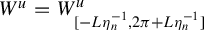 $W^u=W^u_{[-L\eta _n^{-1}, 2\pi + L\eta _n^{-1}]}$
, where the ‘margins’
$W^u=W^u_{[-L\eta _n^{-1}, 2\pi + L\eta _n^{-1}]}$
, where the ‘margins’
 $L\eta _n^{-1}$
will be defined in Notation 2.4 and Definition 2.5.
$L\eta _n^{-1}$
will be defined in Notation 2.4 and Definition 2.5.
In words,
 $\Gamma $
is a Cantor set, consisting of the intersections of the
$\Gamma $
is a Cantor set, consisting of the intersections of the
 $\pi _{x,y}$
-projections of
$\pi _{x,y}$
-projections of
 $W^u$
belonging to different (slightly extended) horizontal cylinders of level 0. It discounts intersections of the projections of
$W^u$
belonging to different (slightly extended) horizontal cylinders of level 0. It discounts intersections of the projections of
 $W^u$
being in the same cylinder of level 0. See Figure 2.
$W^u$
being in the same cylinder of level 0. See Figure 2.
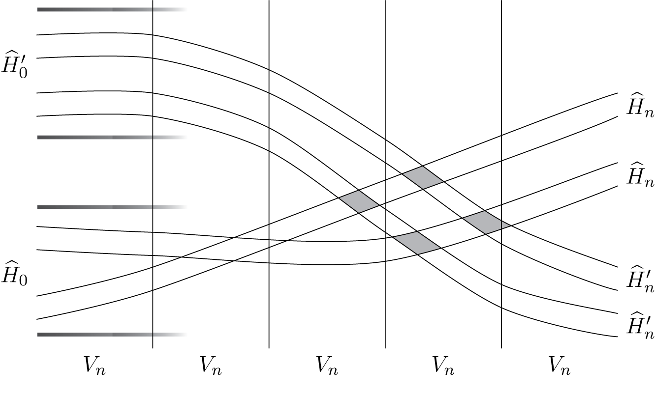
Figure 2 Projection to the
 $(x,y)$
-plane. Here,
$(x,y)$
-plane. Here,
 $H_n=H_{i_{-n},\ldots ,i_0 |}, H^{\prime }_n=H_{i^{\prime }_{-n},\ldots ,i^{\prime }_0 |}, V_n=V_{| i_1,\ldots ,i_n}$
.
$H_n=H_{i_{-n},\ldots ,i_0 |}, H^{\prime }_n=H_{i^{\prime }_{-n},\ldots ,i^{\prime }_0 |}, V_n=V_{| i_1,\ldots ,i_n}$
.
2.1 (Unstable) transversality assumption
All intersections of these lines (that is, projections by
 $\pi _{x,y}$
of unstable manifolds) with different
$\pi _{x,y}$
of unstable manifolds) with different
 $i_0$
values are, in this paper, assumed to be mutually transversal.
$i_0$
values are, in this paper, assumed to be mutually transversal.
Remark 2.3. Notice that by the compactness argument and the continuity of the sub-bundle
 $E^u_{\Lambda }$
, by the transversality assumption, all the intersection angles are bounded away from 0, say by
$E^u_{\Lambda }$
, by the transversality assumption, all the intersection angles are bounded away from 0, say by
 $\alpha _0$
.
$\alpha _0$
.
Also, by compactness and continuity of
 $E^u$
on
$E^u$
on
 $\Lambda $
, there exists
$\Lambda $
, there exists
 $r_0>0$
such that if for
$r_0>0$
such that if for
 $p,p' \in \Lambda \cap W^s$
, their mutual Euclidean distance is
$p,p' \in \Lambda \cap W^s$
, their mutual Euclidean distance is
 $r<r_0$
and their
$r<r_0$
and their
 $i_0$
values are different, then the distance of their
$i_0$
values are different, then the distance of their
 $\pi _{x,y}$
projections from
$\pi _{x,y}$
projections from
 $\Gamma $
, more precisely from the intersection
$\Gamma $
, more precisely from the intersection
 $\widehat W^u(p)\cap \widehat W^u(p')$
, which is in particular non-empty, is bounded by
$\widehat W^u(p)\cap \widehat W^u(p')$
, which is in particular non-empty, is bounded by
 $2r / \tan \alpha _0$
.
$2r / \tan \alpha _0$
.
Remember that we consider f in the form of equation (1.1) and write
 $\eta ':={\partial \eta }/{\partial x}$
,
$\eta ':={\partial \eta }/{\partial x}$
,
 $\unicode{x3bb} ':={\partial \unicode{x3bb} }/{\partial y}$
and
$\unicode{x3bb} ':={\partial \unicode{x3bb} }/{\partial y}$
and
 $\nu ':={\partial \nu }/{\partial z}$
. Then we have the following.
$\nu ':={\partial \nu }/{\partial z}$
. Then we have the following.
Notation 2.4. We write
 $\xi _n^+(p)=\xi (p)\xi (f(p))\ldots \xi (f^n(p))$
for
$\xi _n^+(p)=\xi (p)\xi (f(p))\ldots \xi (f^n(p))$
for
 $\xi =\eta ', \unicode{x3bb} '$
or
$\xi =\eta ', \unicode{x3bb} '$
or
 $\nu '$
. Write also
$\nu '$
. Write also
 $\xi _n^-(p):= \xi _n^+(f^{-n}(p))$
.
$\xi _n^-(p):= \xi _n^+(f^{-n}(p))$
.
Definition 2.5. A point
 $p\in \Lambda $
is said to be strong locally Lipschitz if there is
$p\in \Lambda $
is said to be strong locally Lipschitz if there is
 $L>0$
such that for all n big enough, denoting
$L>0$
such that for all n big enough, denoting
 $(\eta _n^-(p)$
by
$(\eta _n^-(p)$
by
 $\eta _n$
,
$\eta _n$
,
 $$ \begin{align} \operatorname{\mathrm{dist}}(\widehat{V_n(f^{-n}(p))}, \Gamma\cap \widehat{W}^u_{[-L\eta_n^{-1}, 2\pi + L\eta_n^{-1}]}(f^{-n}(p)) \ge L\eta_n^{-1}, \end{align} $$
with the distance in
 ${W}^u$
measured between the projections by
${W}^u$
measured between the projections by
 $\pi _x$
in
$\pi _x$
in
 $\mathbb {R}$
.
$\mathbb {R}$
.
Equivalently, we could replace here
 $\widehat {V_n(f^{-n}(p))}$
by
$\widehat {V_n(f^{-n}(p))}$
by
 $\widehat {f^{-n}(p)}$
. It would influence the constant L only.
$\widehat {f^{-n}(p)}$
. It would influence the constant L only.
By the unstable transversality and transversality of intersection of stable and unstable foliations, this is equivalent to the distance in the
 $\{(x,y)\}$
-plane satisfying
$\{(x,y)\}$
-plane satisfying
 $$ \begin{align} \operatorname{\mathrm{dist}}(\widehat{f^{-n}(p)}, \widehat{W}^u(p') \ge \operatorname{\mathrm{Const}} L \eta_n^{-1} \end{align} $$
for all
 $p'$
having
$p'$
having
 $i_0$
different from the
$i_0$
different from the
 $i_0$
for
$i_0$
for
 $f^{-n}(p)$
.
$f^{-n}(p)$
.
We call all points p which are strong locally Lipschitz with the constant L such that equation (2.2) holds for all
 $q\in W^u(p)$
in place of p strong locally bi-Lipschitz.
$q\in W^u(p)$
in place of p strong locally bi-Lipschitz.
Notice that this definition allows to say that the whole
 $W^u(p)$
is strong locally bi-Lipschitz and write
$W^u(p)$
is strong locally bi-Lipschitz and write
 $$ \begin{align} \operatorname{\mathrm{dist}}(\widehat{f^{-n}(W^u(p))}, \Gamma\cap \widehat{W}^u_{[-L\eta_n^{-1}, 2\pi + L\eta_n^{-1}]} (f^{-n}(p)) \ge L\eta_n^{-1}. \end{align} $$
Remark 2.6. Notice that if for
 $\widehat L>0$
strong locally Lipschitz condition,
$\widehat L>0$
strong locally Lipschitz condition,
 $\operatorname {\mathrm {dist}}(\widehat {f^{-n}(p)}, \Gamma \cap \widehat W^u(f^{-n}(p)))\ge \widehat L \eta _n (f^{-n}(p))^{-1}$
holds and
$\operatorname {\mathrm {dist}}(\widehat {f^{-n}(p)}, \Gamma \cap \widehat W^u(f^{-n}(p)))\ge \widehat L \eta _n (f^{-n}(p))^{-1}$
holds and
 $q\in W^u_{[0,2\pi ]}(p)$
, then
$q\in W^u_{[0,2\pi ]}(p)$
, then
 $\operatorname {\mathrm {dist}}(\widehat {f^{-n}(q)}, \Gamma )\ge (\widehat L - \operatorname {\mathrm {Const}}) \eta _n (f^{-n}(q))^{-1}$
. So for equation (2.2) satisfied at p with
$\operatorname {\mathrm {dist}}(\widehat {f^{-n}(q)}, \Gamma )\ge (\widehat L - \operatorname {\mathrm {Const}}) \eta _n (f^{-n}(q))^{-1}$
. So for equation (2.2) satisfied at p with
 $\widehat L> 2\operatorname {\mathrm {Const}}$
, the strong locally Lipschitz condition holds for all
$\widehat L> 2\operatorname {\mathrm {Const}}$
, the strong locally Lipschitz condition holds for all
 $q\in W^u(p) $
, with
$q\in W^u(p) $
, with
 $L=\widehat L /2$
. So p is strong locally bi-Lipschitz.
$L=\widehat L /2$
. So p is strong locally bi-Lipschitz.
Definition 2.7. For every
 $p\in \Lambda $
and
$p\in \Lambda $
and
 $q\in W^u(p)\setminus \{p\}$
, one defines the holonomy map
$q\in W^u(p)\setminus \{p\}$
, one defines the holonomy map
 $h_{x(p),x(q)}: W^s(p)\to W^s(q)$
along unstable foliation (lamination)
$h_{x(p),x(q)}: W^s(p)\to W^s(q)$
along unstable foliation (lamination)
![]() by
by
 $h_{x(p),x(q)}(v)$
being the only intersection point of
$h_{x(p),x(q)}(v)$
being the only intersection point of
 $W^u(v)$
with
$W^u(v)$
with
 $W^s(q)$
.
$W^s(q)$
.
Theorem 2.8. For every
 $L_2>0$
, there exists
$L_2>0$
, there exists
 $L_1>0$
such that for each p strong locally (bi)Lipschitz with the constant
$L_1>0$
such that for each p strong locally (bi)Lipschitz with the constant
 $L=L_1$
, there exists
$L=L_1$
, there exists
 $n(p)$
such that for each
$n(p)$
such that for each
 $q\in W^u_{[0,2\pi ]} (p)$
, the holonomy between
$q\in W^u_{[0,2\pi ]} (p)$
, the holonomy between
 $W^s(p)\cap \Lambda $
and
$W^s(p)\cap \Lambda $
and
 $W^s(q)\cap \Lambda $
, in
$W^s(q)\cap \Lambda $
, in
 $H_{n(p)}(p)\cap \Lambda $
, is locally bi-Lipschitz continuous at p with Lipschitz constant
$H_{n(p)}(p)\cap \Lambda $
, is locally bi-Lipschitz continuous at p with Lipschitz constant
 $L_2$
.
$L_2$
.
Here, at p means that for every
 $p'\in W^s(p)\cap H_{n(p)}(p)\cap \Lambda $
, we have
$p'\in W^s(p)\cap H_{n(p)}(p)\cap \Lambda $
, we have
 $$ \begin{align*}L_2^{-1}\operatorname{\mathrm{dist}} (p,p') \le \operatorname{\mathrm{dist}} (h_{\pi_x(p),\pi_x(q)}(p), h_{\pi_x(p),\pi_x(q)}(p') \le L_2 \operatorname{\mathrm{dist}} (p,p'), \end{align*} $$
where dist is the euclidean distance in
 $\mathbb {D}$
.
$\mathbb {D}$
.
Proof We repeat (adjust) the calculations in [Reference Hasselblatt, Schmeling, Hasselblatt, Brin and Pesin9]. Consider
 $q\kern1.2pt{\in}\kern1.2pt W^u(p)$
and
$q\kern1.2pt{\in}\kern1.2pt W^u(p)$
and
 ${p'\kern1.2pt{\in}\kern1.2pt W^s(p)\kern1.2pt{\cap}\kern1.2pt \Lambda }$
. Define
${p'\kern1.2pt{\in}\kern1.2pt W^s(p)\kern1.2pt{\cap}\kern1.2pt \Lambda }$
. Define
 $q':= h_{x(p),x(q)} (p')$
. Let
$q':= h_{x(p),x(q)} (p')$
. Let
 $p'\in H_n(p)\setminus H_{n+1}(p)$
, that is,
$p'\in H_n(p)\setminus H_{n+1}(p)$
, that is,
 $p_{-n}=f^{-n}(p)$
and
$p_{-n}=f^{-n}(p)$
and
 $p^{\prime }_{-n}=f^{-n}(p')$
are in different
$p^{\prime }_{-n}=f^{-n}(p')$
are in different
 $H_0$
(Figure 3).
$H_0$
(Figure 3).
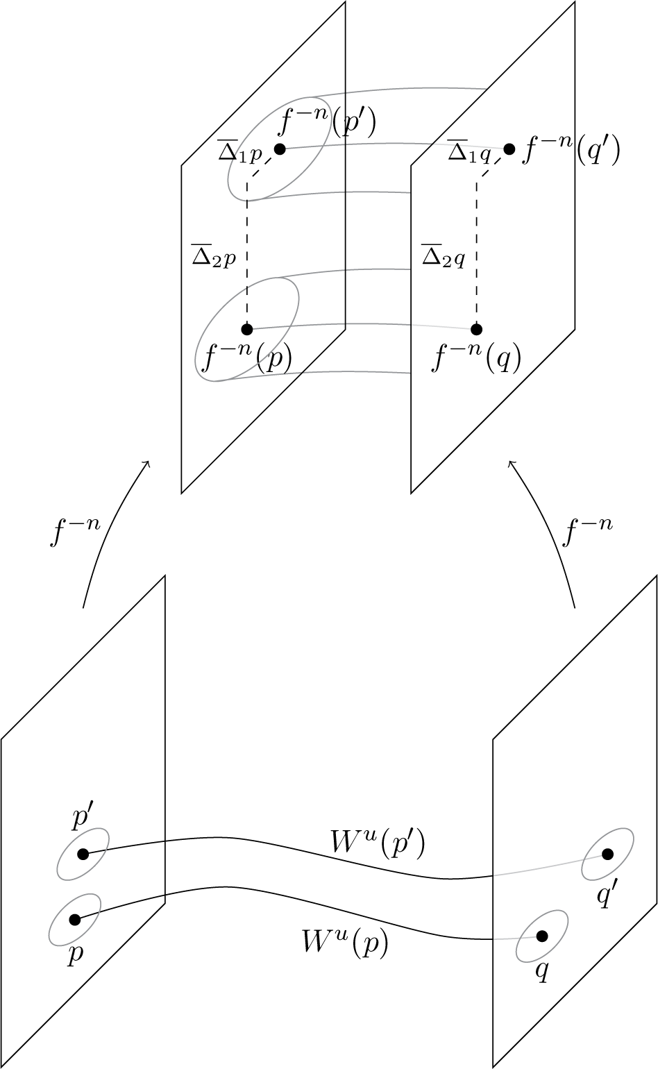
Figure 3 Holonomy twist.
Local Lipschitz continuity of the holonomy
 $h_{x(p),x(q)}$
at p would follow from the existence of a uniform upper bound of
$h_{x(p),x(q)}$
at p would follow from the existence of a uniform upper bound of
 $$ \begin{align} \operatorname{\mathrm{dist}}(q,q') / \operatorname{\mathrm{dist}}(p,p') \end{align} $$
for
 $p'$
close enough to p, that is, n defined above, large.
$p'$
close enough to p, that is, n defined above, large.
It is comfortable to consider the distance
 $d=d_1 + d_2$
, the distances in the y and z coordinates.
$d=d_1 + d_2$
, the distances in the y and z coordinates.
We shall use the triangular form of the differential
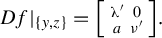 $ Df|_{\{y,z\}} = \Big [\begin {smallmatrix} \unicode{x3bb} ' & 0 \\ a & \nu ' \end {smallmatrix}\Big ]. $
Due to
$ Df|_{\{y,z\}} = \Big [\begin {smallmatrix} \unicode{x3bb} ' & 0 \\ a & \nu ' \end {smallmatrix}\Big ]. $
Due to
 $\nu '<\unicode{x3bb} '$
, we have
$\nu '<\unicode{x3bb} '$
, we have
 $Df^n|_{\{y,z\}}=\Big [\begin {smallmatrix} \unicode{x3bb} _n' & 0 \\ a_n & \nu _n' \end {smallmatrix}\Big ]$
, where
$Df^n|_{\{y,z\}}=\Big [\begin {smallmatrix} \unicode{x3bb} _n' & 0 \\ a_n & \nu _n' \end {smallmatrix}\Big ]$
, where
 $|a_n|\le \operatorname {\mathrm {Const}} \unicode{x3bb} _n$
. Write, according to the decomposition
$|a_n|\le \operatorname {\mathrm {Const}} \unicode{x3bb} _n$
. Write, according to the decomposition
 $d=d_1+d_2$
,
$d=d_1+d_2$
,
 $d(f^{-n}(p),f^{-n}(p')):=\overline \Delta p=\overline \Delta _1 p + \overline \Delta _2 p$
and
$d(f^{-n}(p),f^{-n}(p')):=\overline \Delta p=\overline \Delta _1 p + \overline \Delta _2 p$
and
 $d(f^{-n}(q),f^{-n}(q')):=\overline \Delta q= \overline \Delta _1 q + \overline \Delta _2 q.$
We estimate

for a constant A depending on the angle between
 $W^u$
and
$W^u$
and
 $W^s$
. Here,
$W^s$
. Here,
 $\overline{\unicode{x3bb}} _n, \overline {a_n}, \overline \nu _n$
are averages of derivatives
$\overline{\unicode{x3bb}} _n, \overline {a_n}, \overline \nu _n$
are averages of derivatives
 $\unicode{x3bb} _n,a_n,\nu _n$
, respectively, on appropriate intervals, namely integrals divided by the lengths of the intervals, horizontal along y for two first integrals and vertical along z for the last one.
$\unicode{x3bb} _n,a_n,\nu _n$
, respectively, on appropriate intervals, namely integrals divided by the lengths of the intervals, horizontal along y for two first integrals and vertical along z for the last one.
On the other hand,
To obtain an upper bound of equation (2.5), it is sufficient to assume the existence of an upper bound of the ratio of the above quantities, namely (omitting
 $(f^{-n}(p))$
to simplify notation)
$(f^{-n}(p))$
to simplify notation)

We needed bars over
 $\unicode{x3bb} ,\nu ,a$
to reduce above a fraction to the summand 1. From now on these bars (integrals) are not needed.
$\unicode{x3bb} ,\nu ,a$
to reduce above a fraction to the summand 1. From now on these bars (integrals) are not needed.
We conclude calculations with sufficiency to assume the existence of an upper bound of

or to assume that the inverse
is bounded away from 0.
Thus, Lipschitz property follows from either of
 $$ \begin{align} \overline\Delta_1 p \; \eta_n \ge \operatorname{\mathrm{Const}}> 0 \end{align} $$
or

The condition equation (2.8), in the diagonal case
 $a_n=0$
, means that the contraction in the space of stable leaves
$a_n=0$
, means that the contraction in the space of stable leaves
 $W^s$
by
$W^s$
by
 $f^{-n}$
, along the coordinate x, due to small
$f^{-n}$
, along the coordinate x, due to small
 $\eta _n^{-1}$
is strong enough to bound the twisting effect caused by
$\eta _n^{-1}$
is strong enough to bound the twisting effect caused by
 $\log \nu _n /\log \unicode{x3bb} _n$
, which implies the Lipschitz continuity of all the holonomies at p along unstable foliation of a bounded length leaves (e.g. by
$\log \nu _n /\log \unicode{x3bb} _n$
, which implies the Lipschitz continuity of all the holonomies at p along unstable foliation of a bounded length leaves (e.g. by
 $2\pi $
). This is for
$2\pi $
). This is for
 $\overline \Delta _1(p)\approx 0$
(hence
$\overline \Delta _1(p)\approx 0$
(hence
 $\overline \Delta _2(p)$
large). Otherwise the Lipschitz condition holds automatically.
$\overline \Delta _2(p)$
large). Otherwise the Lipschitz condition holds automatically.
The condition equation (2.7) is equivalent to the strong locally Lipschitz equation (2.2) in Definition 2.5 by the transversality condition, see Remark 2.3 and equations (2.2) and (2.3). This implies that the distance between
 $W^s(f^{-n}(p))$
and
$W^s(f^{-n}(p))$
and
 $W^s(f^{-n}(q))$
is bounded by
$W^s(f^{-n}(q))$
is bounded by
 $\operatorname {\mathrm {Const}}\times \overline \Delta _1(p)$
so
$\operatorname {\mathrm {Const}}\times \overline \Delta _1(p)$
so
 $\overline \Delta _1(q)\le \operatorname {\mathrm {Const}}\overline \Delta _1(p)$
so
$\overline \Delta _1(q)\le \operatorname {\mathrm {Const}}\overline \Delta _1(p)$
so
 $d(q,q')\le \operatorname {\mathrm {Const}} d(p,p')$
so just Lipschitz property of
$d(q,q')\le \operatorname {\mathrm {Const}} d(p,p')$
so just Lipschitz property of
 $h_{p,q}$
at p.
$h_{p,q}$
at p.
By Remark 2.6 for Const above large enough, we obtain a strong bi-Lipschitz property.
We denote the set of all strong locally bi-Lipschitz points in
 $\Lambda $
by
$\Lambda $
by
 $L^s$
and
$L^s$
and
 $L^s\cap W^s(p)$
with
$L^s\cap W^s(p)$
with
 $x(p)=x$
by
$x(p)=x$
by
 $L^s_x$
. Sometimes we write
$L^s_x$
. Sometimes we write
 $\Lambda ^s(\tau , L,n )$
for specified n, see equation (2.2).
$\Lambda ^s(\tau , L,n )$
for specified n, see equation (2.2).
The following has already been mentioned in Theorem 2.8.
Lemma 2.9.
 $h_{x,x'}(L_x^s)=L^s_{x'}$
for all
$h_{x,x'}(L_x^s)=L^s_{x'}$
for all
 $x,x'\in S^1$
for the holonomy
$x,x'\in S^1$
for the holonomy
 $h_{x,x'}$
along unstable foliation. The holonomy is locally Lipschitz on
$h_{x,x'}$
along unstable foliation. The holonomy is locally Lipschitz on
 $L^s$
.
$L^s$
.
Notation 2.10. We call the set complementary to
 $L^{s}$
in
$L^{s}$
in
 $\Lambda $
weak non-Lipschitz, and denote it by
$\Lambda $
weak non-Lipschitz, and denote it by
 $NL^w$
. By Lemma 2.8, this condition is weaker than non-Lipschitz. It includes some Lipschitz (e.g. if the bunching condition holds, see Theorem 1.6).
$NL^w$
. By Lemma 2.8, this condition is weaker than non-Lipschitz. It includes some Lipschitz (e.g. if the bunching condition holds, see Theorem 1.6).
Later on, we shall need the following fact easily following from the definitions.
Lemma 2.11. For every
 $p\in L^s$
, there exists n such that
$p\in L^s$
, there exists n such that
 $$ \begin{align*}W^{ss}(p)\cap\Lambda\cap H_n(p)=\{p\}. \end{align*} $$
Proof Notice that the existence of
 $p'\in W^{ss}(p)\cap \Lambda \cap (H_n(p)\setminus H_{n+1}(p))$
is equivalent to
$p'\in W^{ss}(p)\cap \Lambda \cap (H_n(p)\setminus H_{n+1}(p))$
is equivalent to
 $\pi _{x,y}(f^{-(n+1)}(p))\in \Gamma $
. If it happens for n arbitrarily large, it contradicts
$\pi _{x,y}(f^{-(n+1)}(p))\in \Gamma $
. If it happens for n arbitrarily large, it contradicts
 $p\in L^s$
.
$p\in L^s$
.
3 Lipschitz versus geometric measure
Definition 3.1. Let
 $t=t_0$
be the only zero of the pressure function
$t=t_0$
be the only zero of the pressure function
 $t\mapsto P(f^{-1}, t\log (\unicode{x3bb} ' \circ f^{-1}))$
. Since
$t\mapsto P(f^{-1}, t\log (\unicode{x3bb} ' \circ f^{-1}))$
. Since
 $\unicode{x3bb} '<1$
, this function is strictly decreasing from
$\unicode{x3bb} '<1$
, this function is strictly decreasing from
 $+\infty $
to
$+\infty $
to
 $-\infty $
. Denote by
$-\infty $
. Denote by
 $h^*$
the entropy of the equilibrium measure
$h^*$
the entropy of the equilibrium measure
 $\mu =\mu _{t_0}$
for the potential
$\mu =\mu _{t_0}$
for the potential
 $t_0\log (\unicode{x3bb} \circ f^{-1})$
(called also stable SRB-measure, see §1).
$t_0\log (\unicode{x3bb} \circ f^{-1})$
(called also stable SRB-measure, see §1).
A geometric meaning of this is that for an arbitrary
 $W^s$
, replacing
$W^s$
, replacing
 $\unicode{x3bb} '$
by a function having logarithm cohomologous to
$\unicode{x3bb} '$
by a function having logarithm cohomologous to
 $\log \unicode{x3bb} '$
(denote it also by
$\log \unicode{x3bb} '$
(denote it also by
 $\unicode{x3bb} '$
), not depending on future
$\unicode{x3bb} '$
), not depending on future
 $(|i_1,\ldots )$
, the quantities
$(|i_1,\ldots )$
, the quantities
 $\log \unicode{x3bb} _n (f^{-n}(p))$
for
$\log \unicode{x3bb} _n (f^{-n}(p))$
for
 $p=\rho (\ldots i_0|i_1,\ldots )$
are approximately diameters of
$p=\rho (\ldots i_0|i_1,\ldots )$
are approximately diameters of
 $f^n(W^s(f^{-n}(p)))$
provided
$f^n(W^s(f^{-n}(p)))$
provided
 $\nu ' < \unicode{x3bb} '$
. The quantity
$\nu ' < \unicode{x3bb} '$
. The quantity
 $t_0$
, which would be Hausdorff and box dimensions in the conformal case, here, in the non-conformal case, is only the upper bound of the dimensions of
$t_0$
, which would be Hausdorff and box dimensions in the conformal case, here, in the non-conformal case, is only the upper bound of the dimensions of
 $W^s\cap \Lambda $
, so-called ‘affinity dimension’, [Reference Falconer8]. The aim of this and the next sections is to prove that
$W^s\cap \Lambda $
, so-called ‘affinity dimension’, [Reference Falconer8]. The aim of this and the next sections is to prove that
 $t_0$
is in fact the Hausdorff dimension of all
$t_0$
is in fact the Hausdorff dimension of all
 $W^s\cap \Lambda $
.
$W^s\cap \Lambda $
.
We start now with the following.
Definition 3.2. For each
 ${\underline i}=(i_{-n},\ldots ,i_0)$
, define
${\underline i}=(i_{-n},\ldots ,i_0)$
, define
 $$ \begin{align*} h_n({\underline i})&:= \frac1{n}\log\#\bigg\{(i_1,\ldots,i_n): \widehat H_{i_{-n},\ldots,i_0 |} \cap B(\widehat V_{|i_1,\ldots,i_n}, L_1 {\eta}^{-1}_n( \pi_x \rho({\underline i})))\\ &\qquad\qquad\quad \cap \bigcup_{i^{\prime}_n,\ldots,i^{\prime}_0 \not=i_0}\widehat H_{i^{\prime}_{-n},\ldots,i^{\prime}_0 |} \not=\emptyset \bigg\}, \end{align*} $$
where
 $L_1$
is the constant from Theorem 2.8. Define also
$L_1$
is the constant from Theorem 2.8. Define also
 $$ \begin{align} h_n:=\sup h_n({\underline i}) \;\;\;\; \mathrm{and}\;\;\;\; h:=\limsup h_n. \end{align} $$
Similarly the following.
Definition 3.3. For infinite
 $\underline i=(\ldots ,i_{-n},\ldots ,i_0|)$
and
$\underline i=(\ldots ,i_{-n},\ldots ,i_0|)$
and
 $H_{\underline {i} }=W^u(p)$
for
$H_{\underline {i} }=W^u(p)$
for
 $p\in \rho (\underline {i})$
,
$p\in \rho (\underline {i})$
,
 $$ \begin{align*} h^\infty_n({\underline i}):= \frac1{n}\log\#\{(i_1,\ldots,i_n): \widehat H_{\underline{i}}\cap \widehat V_{| i_1,\ldots,i_n} \cap B(\Gamma\cap \widehat H_{\underline{i}}, L_1 {\eta}^{-1}_n( \pi_x \rho({\underline i})) ) \not=\emptyset\}, \end{align*} $$
compare equation (2.2), and
 $$ \begin{align} h^\infty_n:=\sup h^\infty_n({\underline i}) \;\;\;\; \mathrm{and}\;\;\;\; h^\infty:=\limsup h^\infty_n. \end{align} $$
The following follows easily from the definitions and the transversality assumption.
Proposition 3.4.
 $h^\infty $
and h are independent of
$h^\infty $
and h are independent of
 $L_1$
large enough. Moreover
$L_1$
large enough. Moreover
 $h^\infty \le h$
. The opposite inequality also holds if
$h^\infty \le h$
. The opposite inequality also holds if
 $\sup \unicode{x3bb} '< 1/ \sup \eta '$
and
$\sup \unicode{x3bb} '< 1/ \sup \eta '$
and
 $\nu '(p)<\unicode{x3bb} '(p)$
for every
$\nu '(p)<\unicode{x3bb} '(p)$
for every
 $p\in \Lambda $
, the property we name: uniform dissipation.
$p\in \Lambda $
, the property we name: uniform dissipation.
Lemma 3.5. Assume transversality and
 $\chi _{\mu _{t_0}}(\unicode{x3bb} '))< -\log \sup \eta '$
(call it half-uniform dissipation). Then
$\chi _{\mu _{t_0}}(\unicode{x3bb} '))< -\log \sup \eta '$
(call it half-uniform dissipation). Then
 $$ \begin{align} h^\infty <h^ *. \end{align} $$
Proof For an arbitrary
 $\varepsilon>0$
and n large enough, denoting by
$\varepsilon>0$
and n large enough, denoting by
 $\overline {\operatorname {\mathrm {BD}}}$
the upper box dimension, we easily get
$\overline {\operatorname {\mathrm {BD}}}$
the upper box dimension, we easily get
 $$ \begin{align} h^\infty_n(\underline{i}) \le (\overline{\operatorname{\mathrm{BD}}}(\widehat H_{\underline{i} }\cap\Gamma)+\varepsilon ) ( \log \sup\eta'), \end{align} $$
for every
 $\underline i = \ldots ,i_0 |$
, that is,
$\underline i = \ldots ,i_0 |$
, that is,
 $W^u=W^u(p)$
for any
$W^u=W^u(p)$
for any
 $p\in \rho (\underline i)$
.
$p\in \rho (\underline i)$
.
To prove this, we cover
 $W^u$
by pairwise disjoint (except their end points) arcs of the same length equal to
$W^u$
by pairwise disjoint (except their end points) arcs of the same length equal to
 $1/(\sup \eta ')^n$
(up to a constant) and use the definition of box dimension.
$1/(\sup \eta ')^n$
(up to a constant) and use the definition of box dimension.
A difficulty we shall deal with below is, however, to pass in equation (3.4) to a uniform over
 $\underline {i}$
version, that is, with
$\underline {i}$
version, that is, with
 $\sup _{\underline i} h_n^\infty (\underline i)$
in equation (3.2).
$\sup _{\underline i} h_n^\infty (\underline i)$
in equation (3.2).
Notice that
 $$ \begin{align} \overline{\operatorname{\mathrm{BD}}}(\widehat H_{\underline{i}}\cap\Gamma) \le t_0 &= h^*/(-\chi_{\mu_{t_0}}(\unicode{x3bb}'))\nonumber \\ &\le h^*/(-\sup\log\unicode{x3bb}') < h^* / \log \sup\eta'. \end{align} $$
The first inequality uses the ‘Lipschitz holonomy’ along
![]() (in fact only local) between an arbitrary
(in fact only local) between an arbitrary
 $\widehat W^s$
and
$\widehat W^s$
and
 $\widehat W^u=\widehat W^u(p)$
. (Formally this is not even a holonomy, because of intersections of the leaves. However it is Lipschitz in the sense of varying all the lengths of the uniformly transversal sections of each strip
$\widehat W^u=\widehat W^u(p)$
. (Formally this is not even a holonomy, because of intersections of the leaves. However it is Lipschitz in the sense of varying all the lengths of the uniformly transversal sections of each strip
 $\widehat H_n$
for all n, by at most a common factor.) We shall prove it more precisely below.
$\widehat H_n$
for all n, by at most a common factor.) We shall prove it more precisely below.
Let
 $p'\in W^s \cap \Lambda $
be such that
$p'\in W^s \cap \Lambda $
be such that
 $p'=p'(\underline i')$
is the only point of the intersection
$p'=p'(\underline i')$
is the only point of the intersection
 $\rho (\underline i')\cap W^s$
. Assume that
$\rho (\underline i')\cap W^s$
. Assume that
 $i^{\prime }_0\not =i_0$
. Denote by
$i^{\prime }_0\not =i_0$
. Denote by
 $A(f)$
supremum over all
$A(f)$
supremum over all
 $p,p'$
as above of the number of the intersection points of
$p,p'$
as above of the number of the intersection points of
 $\widehat W^u(p)$
and
$\widehat W^u(p)$
and
 $\widehat W^u(p')$
. It is finite by the transversality assumption, see e.g. [Reference Rams14, Proposition 4.6].
$\widehat W^u(p')$
. It is finite by the transversality assumption, see e.g. [Reference Rams14, Proposition 4.6].
For every
 $n\ge 0$
we have, due to
$n\ge 0$
we have, due to
 $\nu <\unicode{x3bb} $
,
$\nu <\unicode{x3bb} $
,
for n large enough to kill a twisting effect which may be caused by
 ${\partial \nu }/{\partial y}$
. Hence, due to the transversality assumption,
${\partial \nu }/{\partial y}$
. Hence, due to the transversality assumption,
for every component Comp of the intersection.
By the definition of
 $t_0$
we have, summing over all
$t_0$
we have, summing over all
 $(i^{\prime }_{-n},\ldots ,i^{\prime }_0|) $
with
$(i^{\prime }_{-n},\ldots ,i^{\prime }_0|) $
with
 $i_0'\not =i_0$
,
$i_0'\not =i_0$
,

for
 $t>t_0$
and constant
$t>t_0$
and constant
 $C(t)$
or
$C(t)$
or
 $t<t_0$
, respectively.
$t<t_0$
, respectively.
For each
 $r>0$
and
$r>0$
and
 $\widehat q\in \widehat W^u(p))\cap \Gamma $
, where
$\widehat q\in \widehat W^u(p))\cap \Gamma $
, where
 $q\in \rho (\ldots ,i^{\prime }_0|)$
, find
$q\in \rho (\ldots ,i^{\prime }_0|)$
, find
 $n=n(q)$
the least integer such that the length satisfies
$n=n(q)$
the least integer such that the length satisfies
 $l(\widehat W^u\cap \widehat H_{i^{\prime }_{-n},\ldots ,i^{\prime }_0})\le r$
; by the length (denoted above by diam) we mean here the length of the projection by
$l(\widehat W^u\cap \widehat H_{i^{\prime }_{-n},\ldots ,i^{\prime }_0})\le r$
; by the length (denoted above by diam) we mean here the length of the projection by
 $\pi _x$
to
$\pi _x$
to
 $\mathbb {R}$
(of course we can alternatively consider the lengths in
$\mathbb {R}$
(of course we can alternatively consider the lengths in
 $\widehat W^u(p)$
or
$\widehat W^u(p)$
or
 $W^u(p)$
).
$W^u(p)$
).
Denote
 $\widehat W^u\cap \widehat H_{i^{\prime }_{-n},\ldots ,i^{\prime }_0}$
by
$\widehat W^u\cap \widehat H_{i^{\prime }_{-n},\ldots ,i^{\prime }_0}$
by
 $I(q,r)$
. Consider in
$I(q,r)$
. Consider in
 $\widehat W^u$
the ball (arc)
$\widehat W^u$
the ball (arc)
 $J(q,r)=B(\widehat q,r)$
. Choose a family
$J(q,r)=B(\widehat q,r)$
. Choose a family
 $J(q_k,r)$
of the arcs of the form
$J(q_k,r)$
of the arcs of the form
 $J(q,r)$
covering
$J(q,r)$
covering
 $\widehat W^u\cap \Gamma $
, having multiplicity at most 2, namely that each point in
$\widehat W^u\cap \Gamma $
, having multiplicity at most 2, namely that each point in
 $\widehat W^u$
belongs to at most two arcs. Then
$\widehat W^u$
belongs to at most two arcs. Then
 $I(q_k,r)\subset J(q_k,r)$
for all k. On the other hand, by the definition of
$I(q_k,r)\subset J(q_k,r)$
for all k. On the other hand, by the definition of
 $n(q)$
, there is a constant K such that
$n(q)$
, there is a constant K such that
 $K l(I(q_k,r))\ge l(J(q_k,r))$
.
$K l(I(q_k,r))\ge l(J(q_k,r))$
.
Finally notice that for two different
 $q_k$
and
$q_k$
and
 $q_{k'}$
, it may happen that
$q_{k'}$
, it may happen that
 $n=n(k)=n(k')$
and the nth codings
$n=n(k)=n(k')$
and the nth codings
 $i_{-n},\ldots ,i_0$
are the same; in other words, the nth horizontal cylinders coincide. Then however,
$i_{-n},\ldots ,i_0$
are the same; in other words, the nth horizontal cylinders coincide. Then however,
 $J(q_k)$
and
$J(q_k)$
and
 $J(q_{k'})$
intersect so the coincidence of these codings may happen only for at most two different k and
$J(q_{k'})$
intersect so the coincidence of these codings may happen only for at most two different k and
 $k'$
.
$k'$
.
Thus, for all
 $t>t_0$
,
$t>t_0$
,
Hence, as our estimates hold for every
 $r>0$
, we obtain the first inequality in equation (3.4)
$r>0$
, we obtain the first inequality in equation (3.4)
 $$ \begin{align*}\overline{\operatorname{\mathrm{BD}}}( W^u(p)\cap \Gamma) \le t_0. \end{align*} $$
This has been a Moran covering type argument.
Another variant of this proof would be to consider for each n the partition of
 $W^u$
into
$W^u$
into
 $d_n:= 2\pi /r_n$
arcs of length
$d_n:= 2\pi /r_n$
arcs of length
 $r=r_n=1/([\sup {\eta '}^n]+1)$
and consider the family of those arcs which intersect
$r=r_n=1/([\sup {\eta '}^n]+1)$
and consider the family of those arcs which intersect
 $\Gamma $
. Denote them by
$\Gamma $
. Denote them by
 $J_k$
. For each k, choose an arbitrary
$J_k$
. For each k, choose an arbitrary
 $q_k\in \Lambda $
such that
$q_k\in \Lambda $
such that
 $\widehat q_k \in J_k\cap \Gamma $
and
$\widehat q_k \in J_k\cap \Gamma $
and
 $q_k$
belongs to some
$q_k$
belongs to some
 $\rho (\underline i')$
with
$\rho (\underline i')$
with
 $i_0\not =i^{\prime }_0$
. Then consider
$i_0\not =i^{\prime }_0$
. Then consider
 $I_k$
as above. Finally, notice that each interval
$I_k$
as above. Finally, notice that each interval
 $I_k$
, as shorter than
$I_k$
, as shorter than
 $r_n$
for n large enough, can appear at most twice.
$r_n$
for n large enough, can appear at most twice.
Finally, by equation (3.6), the estimate (3.4) is uniform, that is, n for which it holds is independent of
 $\underline i$
. Indeed, for each
$\underline i$
. Indeed, for each
 $\underline i$
and n, we obtain for
$\underline i$
and n, we obtain for
 $r=1/(\sup \eta ')^n$
, denoting
$r=1/(\sup \eta ')^n$
, denoting
 $\varepsilon =2(t-t_0)$
,
$\varepsilon =2(t-t_0)$
,
 $$ \begin{align*}(\exp n h_n^\infty(\underline i)) (2r)^{t_0+\varepsilon} \le (2r)^{\varepsilon/2}\operatorname{\mathrm{Const}} C(t)<1 \end{align*} $$
for n large enough.
So
 $h_n^\infty \le (t_0+\varepsilon )(\sup \eta ')$
for each
$h_n^\infty \le (t_0+\varepsilon )(\sup \eta ')$
for each
 $\varepsilon>0$
and n large enough, hence
$\varepsilon>0$
and n large enough, hence
 $h^\infty \le t_0 \sup \eta '$
. By equation (3.5), we have
$h^\infty \le t_0 \sup \eta '$
. By equation (3.5), we have
 $h^*> t_0 \sup \eta '$
. Thus
$h^*> t_0 \sup \eta '$
. Thus
 $h^\infty < h^*$
.
$h^\infty < h^*$
.
The simplest uniform dissipation, namely if
 ${\eta }^{-1}_n \equiv d^{-n}$
, provides the partitions of
${\eta }^{-1}_n \equiv d^{-n}$
, provides the partitions of
 $S^1$
into arcs of equal lengths to be used in estimating BD. In more general cases, the partitions of
$S^1$
into arcs of equal lengths to be used in estimating BD. In more general cases, the partitions of
 $S^1$
into arcs between consecutive
$S^1$
into arcs between consecutive
 $\eta ^n$
preimages of a fixed point cause difficulties and a necessity to assume the half-uniform dissipation assumption using
$\eta ^n$
preimages of a fixed point cause difficulties and a necessity to assume the half-uniform dissipation assumption using
 $\sup \eta '$
rather than
$\sup \eta '$
rather than
 $\eta '$
. They will be overcome in §4 in the proof of Theorem 4.1 by replacing h by certain
$\eta '$
. They will be overcome in §4 in the proof of Theorem 4.1 by replacing h by certain
 $h^{\mathrm {{reg}}}$
by restricting in the definition to
$h^{\mathrm {{reg}}}$
by restricting in the definition to
 $\mu _{t_0}$
-Birkhoff regular points with respect to
$\mu _{t_0}$
-Birkhoff regular points with respect to
 $\log \eta '$
, restricting
$\log \eta '$
, restricting
 $\Gamma $
.
$\Gamma $
.
Now, assuming the uniform dissipation, using
 $h<h^*$
following from Lemma 3.5 and Proposition 3.4, we can obtain the following.
$h<h^*$
following from Lemma 3.5 and Proposition 3.4, we can obtain the following.
Lemma 3.6. Assume that the transversality and the uniform dissipation condition (introduced in Proposition 3.4) hold. Then
 $\mu ^s_x(L^s)=1$
for
$\mu ^s_x(L^s)=1$
for
 $(\pi _x)_*(\mu )$
-a.e.
$(\pi _x)_*(\mu )$
-a.e.
 $x\in S^1$
, where
$x\in S^1$
, where
 $\mu ^s_x$
are conditional measures of
$\mu ^s_x$
are conditional measures of
 $\mu $
for the partition of
$\mu $
for the partition of
 $\Lambda $
into
$\Lambda $
into
 $W^s_x\cap \Lambda $
.
$W^s_x\cap \Lambda $
.
The same holds for all x, where
 $\mu ^s_x$
is
$\mu ^s_x$
is
 $(h_{x',x})_*(\mu ^s_{x'})$
for
$(h_{x',x})_*(\mu ^s_{x'})$
for
 $x'$
, where
$x'$
, where
 $\mu ^s_{x'}$
has already been defined as a conditional measure.
$\mu ^s_{x'}$
has already been defined as a conditional measure.
Remark that for
 $\mu $
-a.e.
$\mu $
-a.e.
 $p, p'$
the holonomy
$p, p'$
the holonomy
 $h_{x,x'}$
for
$h_{x,x'}$
for
 $x=\pi _x(p), x'=\pi _x(p')$
maps
$x=\pi _x(p), x'=\pi _x(p')$
maps
 $\mu ^s_x$
to
$\mu ^s_x$
to
 $\mu _{x'}^s$
, that is,
$\mu _{x'}^s$
, that is,
 $(h_{x,x'})_*(\mu ^s_x)=\mu ^s_{x'}$
.
$(h_{x,x'})_*(\mu ^s_x)=\mu ^s_{x'}$
.
Note that these measures coincide also with the factor measure
 $\mu ^-:= \Phi _*(\mu _{t_0})$
, where
$\mu ^-:= \Phi _*(\mu _{t_0})$
, where
 $\Phi $
maps the two sides to the one-sided shift to the right, on the space of sequences
$\Phi $
maps the two sides to the one-sided shift to the right, on the space of sequences
 $(\ldots ,i_{-n},\ldots ,i_0)$
(projected to
$(\ldots ,i_{-n},\ldots ,i_0)$
(projected to
 $f^{-1}$
by
$f^{-1}$
by
 $\rho $
). In fact, we can write
$\rho $
). In fact, we can write
 $\mu $
in place of
$\mu $
in place of
 $\mu ^-$
considering its restriction to the
$\mu ^-$
considering its restriction to the
 $\sigma $
-algebra generated by horizontal cylinders.
$\sigma $
-algebra generated by horizontal cylinders.
Then the assertion of Lemma 3.6 says that
 $\mu ^-(\Phi (L^s))=\mu (L^s)=1$
.
$\mu ^-(\Phi (L^s))=\mu (L^s)=1$
.
Proof By the Shannon–McMillan–Breiman theorem [Reference Przytycki and Urbański12] applied for
 $f^{-1}$
and by ergodicity, denoting as before by
$f^{-1}$
and by ergodicity, denoting as before by
 $H_n(p)$
the horizontal cylinder of level n containing p, we get
$H_n(p)$
the horizontal cylinder of level n containing p, we get
 $$ \begin{align*}{1\over n+1}\log \mu( H_n(p))\to h^* \end{align*} $$
for
 $\mu $
-a.e.
$\mu $
-a.e.
 $p\in \Lambda $
, so for every
$p\in \Lambda $
, so for every
 $\varepsilon>0$
and n large enough,
$\varepsilon>0$
and n large enough,
 $$ \begin{align} \exp -(n+1)(h^* + \varepsilon) \le \mu(H_n(p)) \le \exp -(n+1)(h^* - \varepsilon). \end{align} $$
Given arbitrary
 $\varepsilon>0$
and n, denote the set of p values (a union of
$\varepsilon>0$
and n, denote the set of p values (a union of
 $H_n(p)$
values) where equation (3.7) does not hold, by
$H_n(p)$
values) where equation (3.7) does not hold, by
 $Y_{\varepsilon , n}$
. Thus, the irregular set
$Y_{\varepsilon , n}$
. Thus, the irregular set
 $$ \begin{align} Y^{\mathrm{irreg}}_\varepsilon:=\limsup_{n\to\infty}Y_{\varepsilon,n}= \bigcap_n \bigcup_{k\ge n} Y_{\varepsilon,k} \end{align} $$
has measure
 $\mu $
equal to 0. Its
$\mu $
equal to 0. Its
 $\varepsilon $
-regular complement
$\varepsilon $
-regular complement
 $\liminf _{n\to \infty }X_{\varepsilon ,n}= \bigcup _n \bigcap _{k\ge n} X_{\varepsilon ,k}$
for
$\liminf _{n\to \infty }X_{\varepsilon ,n}= \bigcup _n \bigcap _{k\ge n} X_{\varepsilon ,k}$
for
 $X_{\varepsilon .k}=\Lambda \setminus Y_{\varepsilon ,k}$
has full measure
$X_{\varepsilon .k}=\Lambda \setminus Y_{\varepsilon ,k}$
has full measure
 $\mu $
for each
$\mu $
for each
 $\varepsilon $
.
$\varepsilon $
.
Remark that for our Gibbs measure, we can use Birkhoff’s ergodic theorem for
 $f^{-1}$
and
$f^{-1}$
and
 $\log \unicode{x3bb} '$
in place of the Shannon–McMillan–Breiman theorem:
$\log \unicode{x3bb} '$
in place of the Shannon–McMillan–Breiman theorem:
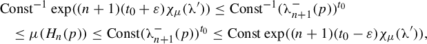 $$ \begin{align*} &\operatorname{\mathrm{Const}}^{-1} \exp ((n+1)(t_0 + \varepsilon )\chi_\mu(\unicode{x3bb}') ) \le \operatorname{\mathrm{Const}}^{-1} (\unicode{x3bb}^-_{n+1} (p))^{t_0} \\ &\quad\le \mu( H_n(p))\le \operatorname{\mathrm{Const}} (\unicode{x3bb}^-_{n+1} (p))^{t_0}\le \operatorname{\mathrm{Const}} \exp ((n+1)(t_0-\varepsilon )\chi_\mu(\unicode{x3bb}') ), \end{align*} $$
where
 $\chi _{\mu }(\unicode{x3bb} ') =\int \log \unicode{x3bb} '\, d\mu $
.
$\chi _{\mu }(\unicode{x3bb} ') =\int \log \unicode{x3bb} '\, d\mu $
.
Denote by
![]() the family of all horizontal cylinders
the family of all horizontal cylinders
 $H_{2n}$
, whose
$H_{2n}$
, whose
 $\pi _{x,y}$
-projections
$\pi _{x,y}$
-projections
 $\widehat H_{2n}$
have ‘horizontal extensions’ to
$\widehat H_{2n}$
have ‘horizontal extensions’ to
 $(-L2\pi , (L+1)2\pi )$
intersecting
$(-L2\pi , (L+1)2\pi )$
intersecting
 $\widehat f^n( \Gamma )$
and else which are in
$\widehat f^n( \Gamma )$
and else which are in
 $X_{\varepsilon ,2n}$
. The constant L is the one that appeared in equation (2.2).
$X_{\varepsilon ,2n}$
. The constant L is the one that appeared in equation (2.2).
Claim 3.7. The upper bound of
![]() is roughly
is roughly
 $\exp (n h + (n+1)h^*)$
(‘roughly’ means: up to a factor of order at most
$\exp (n h + (n+1)h^*)$
(‘roughly’ means: up to a factor of order at most
 $\exp n\varepsilon $
).
$\exp n\varepsilon $
).
Indeed, the number
 $\exp n h$
comes from
$\exp n h$
comes from
 $f^n(H)$
for each
$f^n(H)$
for each
 $H\in H(n)$
, more precisely from
$H\in H(n)$
, more precisely from
 $\widehat {f}^n$
-images of the rectangles
$\widehat {f}^n$
-images of the rectangles
 $\widehat H\cap \widehat V_{|i_1,\ldots ,i_n}$
counted in Definition 3.2. The number
$\widehat H\cap \widehat V_{|i_1,\ldots ,i_n}$
counted in Definition 3.2. The number
 $\exp (n+1)h^*$
comes from the number of ‘regular’
$\exp (n+1)h^*$
comes from the number of ‘regular’
 $H\in H(n)$
roughly as in equation (3.7), that is, being
$H\in H(n)$
roughly as in equation (3.7), that is, being
 $f^{n+1}$
-images of ‘regular’
$f^{n+1}$
-images of ‘regular’
 $V_n$
. More precisely, of those H values for which some
$V_n$
. More precisely, of those H values for which some
 $H_{2n+1}\subset f^n(H)$
are in
$H_{2n+1}\subset f^n(H)$
are in
 $X_{\varepsilon ,2n+1}\cap X_{\varepsilon ,n}$
. (Notice that this does not depend on the choice of
$X_{\varepsilon ,2n+1}\cap X_{\varepsilon ,n}$
. (Notice that this does not depend on the choice of
 $H_{2n+1}$
, due to equation (3.9). Notice also that H satisfying this, need not exhaust all H satisfying equation (3.7).) The measure
$H_{2n+1}$
, due to equation (3.9). Notice also that H satisfying this, need not exhaust all H satisfying equation (3.7).) The measure
 $\mu $
of each such H is lower bounded for
$\mu $
of each such H is lower bounded for
 $p\in H$
by
$p\in H$
by
 $$ \begin{align} &\operatorname{\mathrm{Const}} \unicode{x3bb}^-_{n+1}(p)^{t_0} = \operatorname{\mathrm{Const}} \unicode{x3bb}^-_{2n+1}(f^n(p))^{t_0} / \unicode{x3bb}^-_n(f^n(p))^{t_0} \nonumber\\ &\quad\ge \exp ((n+1) \chi_\mu(\unicode{x3bb}')-(3n+1)\varepsilon)t_0 = \exp (- (n+1) h^*) \exp (- (3n+1) \varepsilon t_0 ), \end{align} $$
due to chain rule
 $f^{-(n+1)}(p) = f^{-2n+1} (f^n(p)) \circ f^n(p)$
, compare equation (4.4), and Gibbs property of
$f^{-(n+1)}(p) = f^{-2n+1} (f^n(p)) \circ f^n(p)$
, compare equation (4.4), and Gibbs property of
 $\mu $
(used already above to reformulate equation (3.7) to the language of
$\mu $
(used already above to reformulate equation (3.7) to the language of
 $\unicode{x3bb} '$
).
$\unicode{x3bb} '$
).
The number of our ‘regular’
 $H_n$
values is bounded by the reciprocal of the bound in equation (3.9). Thus,
$H_n$
values is bounded by the reciprocal of the bound in equation (3.9). Thus,
The claim has been proven.
Thus,
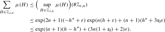
So, for an arbitrary
 $\varepsilon>0$
small enough,
$\varepsilon>0$
small enough,

so
 $\mu (NL^w)=0$
, see Notation 2.10.
$\mu (NL^w)=0$
, see Notation 2.10.
4 Hausdorff dimension
Theorem 4.1. (Theorem 1.2)
Assume
 $\chi _{\mu }(\nu ')<\chi _{\mu } (\unicode{x3bb} ')< -\chi _{\mu }(\eta ')$
. Then, for
$\chi _{\mu }(\nu ')<\chi _{\mu } (\unicode{x3bb} ')< -\chi _{\mu }(\eta ')$
. Then, for
 $\operatorname {\mathrm {HD}}$
denoting the Hausdorff dimension, for
$\operatorname {\mathrm {HD}}$
denoting the Hausdorff dimension, for
 $\Lambda _x$
denoting
$\Lambda _x$
denoting
 $\Lambda \cap (\{x\}\times \mathbb {D})=\Lambda \cap W^s_x$
:
$\Lambda \cap (\{x\}\times \mathbb {D})=\Lambda \cap W^s_x$
:
-
(1)
$\operatorname {\mathrm {HD}}(\Lambda _x)=t_0$
for every x; and -
(2)
$\operatorname {\mathrm {HD}}(\Lambda )=1+t_0$
, where
$t_0= {h^*/-\chi _{\mu _{t_0}}(\unicode{x3bb} ')}$
.

First, we prove this theorem under stronger assumptions.
Theorem 4.2. (Theorem 1.2, uniformly dissipative setting)
Assertions of Theorem 4.1 hold if
 $\sup \unicode{x3bb} ' < 1/\sup \eta '$
.
$\sup \unicode{x3bb} ' < 1/\sup \eta '$
.
We start with a general (not only in the uniformly dissipative) case.
Lemma 4.3. For every
 $p\in \Lambda $
, all
$p\in \Lambda $
, all
 $r>0$
and balls (discs)
$r>0$
and balls (discs)
 $B^s$
in the stable manifold
$B^s$
in the stable manifold
 $W^s_{\pi _x(p)}$
,
$W^s_{\pi _x(p)}$
,
 $$ \begin{align*}\mu^s_{\pi_x(p)}(B^s(p,r)) \ge \operatorname{\mathrm{Const}} (\operatorname{\mathrm{diam}} B^s(p,r))^{ t_0}. \end{align*} $$
In particular,
 $$ \begin{align*}\liminf_{r\to 0} {\log\mu^s_{\pi_{x(p)}}(B^s(p,r)) \over \log \operatorname{\mathrm{diam}} (B^s(p,r))}\le t_0. \end{align*} $$
One can even replace liminf by limsup.
Proof Lemma 4.3 follows from
One uses the definition of
 $\mu ^s$
(Gibbs property) and the fact that the diameter of each
$\mu ^s$
(Gibbs property) and the fact that the diameter of each
 $B^s(p,r)$
is comparable to
$B^s(p,r)$
is comparable to
 $\unicode{x3bb} _n(f^{-n}(p))$
, by bounded distortion. The conditional measures
$\unicode{x3bb} _n(f^{-n}(p))$
, by bounded distortion. The conditional measures
 $\mu ^s$
were discussed after the statement of Lemma 3.6.
$\mu ^s$
were discussed after the statement of Lemma 3.6.
More sophisticated is the opposite inequality.
Lemma 4.4. For
 $\mu $
-a.e.
$\mu $
-a.e.
 $p\in \Lambda $
, the local dimension satisfies
$p\in \Lambda $
, the local dimension satisfies
 $$ \begin{align*}\delta^s:=\liminf_{r\to 0} {\log\mu^s_{\pi_{x(p)}}(B^s(p,r)) \over \log \operatorname{\mathrm{diam}} (B^s(p,r)}\ge t_0. \end{align*} $$
Proof One uses the Ledrappier–Young formula [Reference Ledrappier and Young10]
 $$ \begin{align*}h_\mu(f)=\delta^{ss} (-\chi_{\mu}(\nu')) + (\delta^s-\delta^{ss}) (-\chi_\mu(\unicode{x3bb}')) \end{align*} $$
and the fact that
 $\delta ^{ss}=0$
since for
$\delta ^{ss}=0$
since for
 $p\in L^s$
the local manifold
$p\in L^s$
the local manifold
 $W^{ss}$
consists only of the point p, see Lemma 2.11. Remember also, Lemma 3.6, that
$W^{ss}$
consists only of the point p, see Lemma 2.11. Remember also, Lemma 3.6, that
 $\mu _x^s(L^s)=1$
for all
$\mu _x^s(L^s)=1$
for all
 $x\in S^1$
, so
$x\in S^1$
, so
 $\mu (L^s)=1$
. Hence,
$\mu (L^s)=1$
. Hence,
 $$ \begin{align*}h_\mu(f)=\delta^{s} (-\chi_{\mu}(\unicode{x3bb}')),\; \; \mathrm{so} \; \delta^s= h_\mu(f)/-\chi_\mu(\unicode{x3bb}')= t_0.\\[-36pt] \end{align*} $$
Proof of Theorem 1.2, uniformly dissipative setting
Step 1.
 $\operatorname {\mathrm {HD}}(\Lambda _x)=t_0$
for every x follows from Lemmas 4.3 and 4.4 and from Frostman Lemma, see [Reference Przytycki and Urbański12, Theorem 8.6.3].
$\operatorname {\mathrm {HD}}(\Lambda _x)=t_0$
for every x follows from Lemmas 4.3 and 4.4 and from Frostman Lemma, see [Reference Przytycki and Urbański12, Theorem 8.6.3].
Step 2. Since by Lemma 3.5 and Proposition 3.4
 $h<h^*:=h_{\mu _{t_0}}(f)$
, we know by Lemma 3.6 that there exists x (in fact for all x)
$h<h^*:=h_{\mu _{t_0}}(f)$
, we know by Lemma 3.6 that there exists x (in fact for all x)
 $\mu ^s_x(L^s)=1$
. By Lemma 2.9, all the holonomies
$\mu ^s_x(L^s)=1$
. By Lemma 2.9, all the holonomies
 $h_{x,x'}$
for
$h_{x,x'}$
for
 $0\le x'\le 2\pi $
are locally bi-Lipschitz on
$0\le x'\le 2\pi $
are locally bi-Lipschitz on
 $L^s(x)$
. Change the coordinates on
$L^s(x)$
. Change the coordinates on
 $\Lambda $
by
$\Lambda $
by
 $F(x', y, z):= (x',h_{x,x'}^{-1}(y,z))$
, mapping
$F(x', y, z):= (x',h_{x,x'}^{-1}(y,z))$
, mapping
 $\Lambda $
to the cartesian product
$\Lambda $
to the cartesian product
 $[0,2\pi ) \times \Lambda \cap W^s_x$
. Then this change is locally Lipschitz on
$[0,2\pi ) \times \Lambda \cap W^s_x$
. Then this change is locally Lipschitz on
 $\bigcup _{0\le x' \le 2\pi }h_{x,x'}(L^s_x)=L^s$
. Hence,
$\bigcup _{0\le x' \le 2\pi }h_{x,x'}(L^s_x)=L^s$
. Hence,
 $\operatorname {\mathrm {HD}}(\Lambda )\ge \operatorname {\mathrm {HD}}(L^s)=1+HD(L^s_x)= 1+t_0$
.
$\operatorname {\mathrm {HD}}(\Lambda )\ge \operatorname {\mathrm {HD}}(L^s)=1+HD(L^s_x)= 1+t_0$
.
More precisely, F is locally Lipschitz, in the sense that there exists
 $L>0$
such that for every
$L>0$
such that for every
 $p\in L^s$
, there exists measurable
$p\in L^s$
, there exists measurable
 $r(p)>0$
such that for every
$r(p)>0$
such that for every
 $r\le r(p)$
and
$r\le r(p)$
and
 $q\in B(p,r)$
,
$q\in B(p,r)$
,
 $\operatorname {\mathrm {dist}} (F(p), F(q)) \le L \operatorname {\mathrm {dist}} (p,q)$
. This is sufficient to not increase dimension by splitting the space into a countable number of pieces.
$\operatorname {\mathrm {dist}} (F(p), F(q)) \le L \operatorname {\mathrm {dist}} (p,q)$
. This is sufficient to not increase dimension by splitting the space into a countable number of pieces.
Step 3. The opposite inequality is implied by Lemma 4.3. Indeed, notice that for every
 $r=\unicode{x3bb} _n(p)$
and
$r=\unicode{x3bb} _n(p)$
and
 $x'\in B(x(p), r)$
, we have
$x'\in B(x(p), r)$
, we have
 $$ \begin{align*}\{x'\} \times B^s(\pi_{y,z}(p), (C+1)\cdot r)\supset h_{x(p),x'}(B^s(\pi_{y,z},r), \end{align*} $$
where
 $C:= \tan \measuredangle (E^u,E^s)$
. Hence
$C:= \tan \measuredangle (E^u,E^s)$
. Hence
 $$ \begin{align*}\mu^s(\{x'\} \times B^s(\pi_{y,z}(p), (C+1)\cdot r))\ge \mu^s h_{x(p),x'}(B^s(\pi_{y,z},r). \end{align*} $$
Hence, for
 $$ \begin{align} \widehat\mu:=d\mu^s_x d\operatorname{\mathrm{Leb}}_1(x), \end{align} $$
for every
 $p\in \Lambda $
,
$p\in \Lambda $
,
and in conclusion,
 $\widehat \mu (B(p,Cr))\ge \operatorname {\mathrm {Const}} r^{1+t_0}$
yielding the required upper estimate
$\widehat \mu (B(p,Cr))\ge \operatorname {\mathrm {Const}} r^{1+t_0}$
yielding the required upper estimate
 $\operatorname {\mathrm {HD}}(\Lambda )\le 1+t_0$
.
$\operatorname {\mathrm {HD}}(\Lambda )\le 1+t_0$
.
Definition 4.5. A point
 $p=\rho (\ldots i_{-n},\ldots ,i_0,\ldots ,i_n,\ldots )\in \Lambda $
is said to be Birkhoff
$p=\rho (\ldots i_{-n},\ldots ,i_0,\ldots ,i_n,\ldots )\in \Lambda $
is said to be Birkhoff
 $(\xi , \varepsilon , N)$
-backward regular for an arbitrary
$(\xi , \varepsilon , N)$
-backward regular for an arbitrary
 $\varepsilon>0$
and for
$\varepsilon>0$
and for
 $\xi =\nu ,\unicode{x3bb} $
or
$\xi =\nu ,\unicode{x3bb} $
or
 $\eta $
, if for all
$\eta $
, if for all
 $n\ge N$
,
$n\ge N$
,
 $$ \begin{align} \exp n(\chi_\mu(\xi)-\varepsilon) \le \xi_n^-(p)) \le \exp n(\chi_\mu(\xi)+\varepsilon)), \end{align} $$
see Notation 2.4.
Analogously
 $p\in \Lambda $
is said to be Birkhoff
$p\in \Lambda $
is said to be Birkhoff
 $(\xi , \varepsilon , N)$
-forward regular if the above estimates hold for
$(\xi , \varepsilon , N)$
-forward regular if the above estimates hold for
 $\xi _n^+(p)$
in place of
$\xi _n^+(p)$
in place of
 $\xi _n^-(p)$
.
$\xi _n^-(p)$
.
When we mean just equation (4.3), we say
 $(\xi , \varepsilon , n)$
-forward (backward) regular, omitting “Birkhoff”. Compare the Shannon–McMillan–Breiman property in the proof of Lemma 3.6.
$(\xi , \varepsilon , n)$
-forward (backward) regular, omitting “Birkhoff”. Compare the Shannon–McMillan–Breiman property in the proof of Lemma 3.6.
By bounded distortion, the property (4.3) for
 $p=\rho (\ldots i_{-n},\ldots ,i_0,\ldots ,i_n,\ldots )$
depends only on
$p=\rho (\ldots i_{-n},\ldots ,i_0,\ldots ,i_n,\ldots )$
depends only on
 $(i_{-n},\ldots ,i_0)$
, provided we insert constant factors before exp, so it can be considered as a property of a horizontal cylinder
$(i_{-n},\ldots ,i_0)$
, provided we insert constant factors before exp, so it can be considered as a property of a horizontal cylinder
 $H_n$
. Analogously for the forward regularity, this is a property of vertical cylinders
$H_n$
. Analogously for the forward regularity, this is a property of vertical cylinders
 $V_n$
. We call these cylinders
$V_n$
. We call these cylinders
 $(\xi , \varepsilon , n)$
-forward or backward regular, and all other points or level n cylinders irregular.
$(\xi , \varepsilon , n)$
-forward or backward regular, and all other points or level n cylinders irregular.
Proof of Theorem 1.2. We shall modify (generalize) the definition of irregular sets
 $Y_{\varepsilon ,n}$
in Lemma 3.6 and follow the strategy of the proof of that lemma.
$Y_{\varepsilon ,n}$
in Lemma 3.6 and follow the strategy of the proof of that lemma.
Recall the notation
 $\xi _n^-(p):= \xi _n(f^{-n}(p))$
. Notice that for all integers
$\xi _n^-(p):= \xi _n(f^{-n}(p))$
. Notice that for all integers
 $m>0$
,
$m>0$
,
 $$ \begin{align} \xi_m^-(f^{-n}(p) = \xi_{n+m}^-(p) / \xi_{n}^-(p), \end{align} $$
so for p being
 $(\xi ,\varepsilon , k)$
-backward regular for
$(\xi ,\varepsilon , k)$
-backward regular for
 $k=n$
and
$k=n$
and
 $k=n+m$
, we have
$k=n+m$
, we have
 $$ \begin{align*} &\exp (n+m)(\chi_\mu(\xi)-\varepsilon)) / \exp n(\chi_\mu(\xi)+\varepsilon)) \le \xi_m^-(f^{-n}(p) \\[-3pt] &\quad\le \exp (n+m)(\chi_\mu(\xi)+\varepsilon)) / \exp n (\chi_\mu(\xi)-\varepsilon)). \end{align*} $$
Hence
 $$ \begin{align} \exp m \bigg(\frac{n+m}m (\chi_\mu(\xi)-\varepsilon) - \frac{n}m (\chi_\mu(\xi)+\varepsilon)\bigg) \le \xi_m^-(f^{-n})(p)\le \cdots. \end{align} $$
Hence
 $$ \begin{align} \exp m \bigg(\chi_\mu(\xi)-\varepsilon\bigg(2\frac{n}m + 1\bigg)\bigg) \le \xi_m^-(f^{-n}(p)) \le \exp m \bigg(\chi_\mu(\xi)+\varepsilon\bigg(2\frac{n}m + 1\bigg)\bigg). \end{align} $$
For each
 $n,m\in \mathbb {N}$
denote by
$n,m\in \mathbb {N}$
denote by
 $X_{\varepsilon ,n,m}$
the union of all
$X_{\varepsilon ,n,m}$
the union of all
 $H_{n+m}$
horizontal cylinders of
$H_{n+m}$
horizontal cylinders of
 $(\xi ,\varepsilon ,n)$
-backward regular points in
$(\xi ,\varepsilon ,n)$
-backward regular points in
 $\Lambda $
for all
$\Lambda $
for all
 $\xi =\nu ,\unicode{x3bb} $
and
$\xi =\nu ,\unicode{x3bb} $
and
 $\eta $
, and yet
$\eta $
, and yet
 $(\unicode{x3bb} ,\varepsilon ,n+m)$
-backward regular.
$(\unicode{x3bb} ,\varepsilon ,n+m)$
-backward regular.
Write also
 $Y_{\varepsilon ,n,m}:=\Lambda \setminus X_{\varepsilon ,n,m}$
for irregular sets. Now, as in §3, in the proof of Lemma 3.6, the idea is to remove (due to the uniform dissipation assumption, we needed to remove there less than here) for each n the irregular set
$Y_{\varepsilon ,n,m}:=\Lambda \setminus X_{\varepsilon ,n,m}$
for irregular sets. Now, as in §3, in the proof of Lemma 3.6, the idea is to remove (due to the uniform dissipation assumption, we needed to remove there less than here) for each n the irregular set
 $Y_{\varepsilon ,n,m}$
for m to be defined later on, and estimate the number of remaining cylinders
$Y_{\varepsilon ,n,m}$
for m to be defined later on, and estimate the number of remaining cylinders
 $H_{n+m}$
, which are regular contaminated by other regular cylinders in the sense below in equation (4.7).
$H_{n+m}$
, which are regular contaminated by other regular cylinders in the sense below in equation (4.7).
A point (and cylinder)
 $p\in H_{n+m}$
regular as above is said to be
$p\in H_{n+m}$
regular as above is said to be
 $(\Gamma ^{\operatorname {\mathrm {reg}}}_{n,m})$
-contaminated if for
$(\Gamma ^{\operatorname {\mathrm {reg}}}_{n,m})$
-contaminated if for
 ${\tilde p}:=f^{-n}(p)$
 $$ \begin{align} \pi_{x,y}({\tilde p})\in B^u(\Gamma^{\operatorname{\mathrm{reg}}}, L_1 {\eta}^{-1}_n(\tilde p)), \end{align} $$
compare Definition 2.5. Here
 $B^u$
denotes a ball in
$B^u$
denotes a ball in
 ${\widehat W}^u(\tilde p)$
. The set
${\widehat W}^u(\tilde p)$
. The set
 $\Gamma ^{\operatorname {\mathrm {reg}}}$
is defined as
$\Gamma ^{\operatorname {\mathrm {reg}}}$
is defined as
 $\Gamma $
in Definition 2.2, but restricted to
$\Gamma $
in Definition 2.2, but restricted to
 $\widehat p$
being a
$\widehat p$
being a
 $\pi _{x,y}$
image of
$\pi _{x,y}$
image of
 $q=\rho (\ldots ,i_0|)$
and
$q=\rho (\ldots ,i_0|)$
and
 $q'=\rho (\ldots ,i^{\prime }_0|)$
such that
$q'=\rho (\ldots ,i^{\prime }_0|)$
such that
 $f^n(q)$
and
$f^n(q)$
and
 $f^n(q')$
are in
$f^n(q')$
are in
 $X_{\varepsilon ,n,m}$
.
$X_{\varepsilon ,n,m}$
.
As in Definition 2.5, we can say equivalently that
 $\widehat V_n(\tilde p)$
is
$\widehat V_n(\tilde p)$
is
 $\Gamma ^{\operatorname {\mathrm {reg}}}_{n,m}$
-contaminated if it does not satisfy equation (2.2), with
$\Gamma ^{\operatorname {\mathrm {reg}}}_{n,m}$
-contaminated if it does not satisfy equation (2.2), with
 $\Gamma $
replaced by
$\Gamma $
replaced by
 $\Gamma ^{\operatorname {\mathrm {reg}}}_{n,m}$
. We can say also that the rectangle
$\Gamma ^{\operatorname {\mathrm {reg}}}_{n,m}$
. We can say also that the rectangle
 $\widehat H_m \cap \widehat V_n$
is contaminated, as in Definition 3.2. See also §7.4.
$\widehat H_m \cap \widehat V_n$
is contaminated, as in Definition 3.2. See also §7.4.
Here it is comfortable to look for
 $m>0$
as small as possible so that
$m>0$
as small as possible so that
 $$ \begin{align} \unicode{x3bb}^-_m(f^{-n}(p) < (\eta^-_n(p))^{-1}, \end{align} $$
compare equation (5.3) later on. Taking into account that both
 $f^n(q)$
and q are in
$f^n(q)$
and q are in
 $X_{\varepsilon ,n,m}$
, we obtain using equation (4.6) the sufficient condition
$X_{\varepsilon ,n,m}$
, we obtain using equation (4.6) the sufficient condition
 $$ \begin{align*}\exp m \bigg(\chi_\mu(\unicode{x3bb})+\varepsilon\bigg(2\frac{n}{m} + 1\bigg)\bigg) < \exp n (-\chi_\mu(\eta)-\varepsilon). \end{align*} $$
It follows that for
 $\epsilon>0$
small, it is sufficient
$\epsilon>0$
small, it is sufficient
 $$ \begin{align} m/n \approx \chi_\mu(\eta')/(-\chi_\mu(\unicode{x3bb}')) + \varepsilon' \end{align} $$
with
 $\varepsilon '>0$
also small.
$\varepsilon '>0$
also small.
Summarizing: for given
 $H_m(\tilde p)$
with
$H_m(\tilde p)$
with
 $p=f^n(\tilde p)\in X_{\varepsilon ,n,m}$
, we define
$p=f^n(\tilde p)\in X_{\varepsilon ,n,m}$
, we define
 $h^{\operatorname {\mathrm {reg}}}_n:=1/({n+1})\log Z_n$
, where
$h^{\operatorname {\mathrm {reg}}}_n:=1/({n+1})\log Z_n$
, where
 $Z_n$
is the number of
$Z_n$
is the number of
 $\Gamma ^{\operatorname {\mathrm {reg}}}_{n,m}$
-contaminated
$\Gamma ^{\operatorname {\mathrm {reg}}}_{n,m}$
-contaminated
 $\widehat V_n$
in
$\widehat V_n$
in
 $\widehat H_m(\tilde p)$
(by
$\widehat H_m(\tilde p)$
(by
 $H_m(\tilde q)$
with the
$H_m(\tilde q)$
with the
 $i_0$
symbols different from that for
$i_0$
symbols different from that for
 $H_m(\tilde p)$
, with
$H_m(\tilde p)$
, with
 $q=f^n(\tilde q)\in X_{\varepsilon ,n,m}$
).
$q=f^n(\tilde q)\in X_{\varepsilon ,n,m}$
).
The number
 $Z_n$
is bounded by a constant times the number of
$Z_n$
is bounded by a constant times the number of
 $H_m$
above, taking into account L in equation (2.2) and the observation that regular
$H_m$
above, taking into account L in equation (2.2) and the observation that regular
 $H_m$
, as ‘thinner’ than
$H_m$
, as ‘thinner’ than
 $V_m$
, can intersect at most two (neighbour)
$V_m$
, can intersect at most two (neighbour)
 $V_m$
values.
$V_m$
values.
Hence
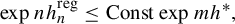 $$ \begin{align*}\exp n h^{\operatorname{\mathrm{reg}}}_n \le \operatorname{\mathrm{Const}} \exp m h^*, \end{align*} $$
so using equation (4.9),
 $$ \begin{align} h^{\operatorname{\mathrm{reg}}}\le h^* (\chi_\mu(\eta')/(-\chi_\mu(\unicode{x3bb}'))) + \varepsilon'. \end{align} $$
The rest of the proof repeats the proof of Theorem 4.2.
In particular, by Birkhoff ergodic theorem for an arbitrary
 $\varepsilon{\kern1pt>\kern1pt}0$
,
$\varepsilon{\kern1pt>\kern1pt}0$
,
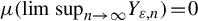 $\mu (\lim \sup _{n\to \infty }\! Y_{\varepsilon ,n}){\kern1pt=\kern1pt}0$
and the complementary set in
$\mu (\lim \sup _{n\to \infty }\! Y_{\varepsilon ,n}){\kern1pt=\kern1pt}0$
and the complementary set in
 $NL^w$
, for
$NL^w$
, for
 $\varepsilon>0$
small enough, where
$\varepsilon>0$
small enough, where
 $h^{\operatorname {\mathrm {reg}}}<h^*$
, has measure
$h^{\operatorname {\mathrm {reg}}}<h^*$
, has measure
 $\mu $
also equal to 0.□
$\mu $
also equal to 0.□
The above proof finishes also the proof of Theorem 1.6 in the general setting, saying that
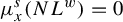 $\mu _x^s(NL^w)=0$
, compare Lemma 3.6 in the uniform dissipation case. Compare also equation (3.8).
$\mu _x^s(NL^w)=0$
, compare Lemma 3.6 in the uniform dissipation case. Compare also equation (3.8).
5 Packing measure
For the definition of packing measure, we refer the reader to [Reference Przytycki and Urbański12, §8.3]. Denote packing measure in dimension t by
 $\Pi _t$
.
$\Pi _t$
.
We shall prove the following.
Theorem 5.1. Under the assumptions of Theorem 4.1 (Theorem 1.2), namely if
 $$ \begin{align*}\chi_{\mu}(\nu')<\chi_{\mu} (\unicode{x3bb}')< -\chi_{\mu}(\eta'), \end{align*} $$
for the Gibbs measure
 $\mu =\mu _{t_0}$
on
$\mu =\mu _{t_0}$
on
 $\Lambda $
, then for every
$\Lambda $
, then for every
 $p\in \Lambda $
, it holds that
$p\in \Lambda $
, it holds that
 $$ \begin{align} 0<\Pi_{t_0}(W^s(p)\cap \Lambda)<\infty. \end{align} $$
Moreover, the density
 $d\Pi _{t_0}/d\mu ^s_{t_0}$
is positive
$d\Pi _{t_0}/d\mu ^s_{t_0}$
is positive
 $\mu ^s_{\pi _x(p)}$
almost everywhere (recall that
$\mu ^s_{\pi _x(p)}$
almost everywhere (recall that
 $\mu ^s_{\pi _x(p)}$
is the conditional measure on
$\mu ^s_{\pi _x(p)}$
is the conditional measure on
 $W^s(p)$
).
$W^s(p)$
).
Also,
 $$ \begin{align} 0<\Pi_{1+t_0}(\Lambda)<\infty \end{align} $$
and moreover
 $d\Pi _{t_0+1}/d\mu _{t_0}$
is positive
$d\Pi _{t_0+1}/d\mu _{t_0}$
is positive
 $\mu _{t_0}$
almost everywhere on
$\mu _{t_0}$
almost everywhere on
 $\Lambda $
.
$\Lambda $
.
This generalizes the analogous theorem proved for linear solenoids in [Reference Rams and Simon17].
Proof
Step 1. Regular contaminated rectangles. Given an arbitrary
 $\varepsilon>0$
, denote by
$\varepsilon>0$
, denote by
 $\mathcal {H}(\varepsilon ,t)$
the union of all
$\mathcal {H}(\varepsilon ,t)$
the union of all
 $H_t$
containing points in
$H_t$
containing points in
 $\Lambda $
satisfying the backward regularity condition in equation (4.3) for t (denoted there n) and
$\Lambda $
satisfying the backward regularity condition in equation (4.3) for t (denoted there n) and
 $\xi =\unicode{x3bb} ,\nu $
.
$\xi =\unicode{x3bb} ,\nu $
.
Analogously, denote by
![]() the union of all
the union of all
 $V_t$
containing points in
$V_t$
containing points in
 $\Lambda $
satisfying the forward regularity condition analogous to equation (4.3) for t (denoted there by n) and
$\Lambda $
satisfying the forward regularity condition analogous to equation (4.3) for t (denoted there by n) and
 $\xi =\eta $
and by
$\xi =\eta $
and by
![]() .
.
We sometimes call
 $H_t$
and
$H_t$
and
 $V_t$
as above, just regular.
$V_t$
as above, just regular.
Consider an arbitrary
 $m\in \mathbb {N}$
and given
$m\in \mathbb {N}$
and given
 $\varepsilon>0$
, define
$\varepsilon>0$
, define
 $n=n(\varepsilon ,m)$
as the biggest integer n such that, compare equations (4.9) and (4.8),
$n=n(\varepsilon ,m)$
as the biggest integer n such that, compare equations (4.9) and (4.8),
 $$ \begin{align} \frac{n}{m} \le \frac{-(\chi_\mu (\unicode{x3bb}')-\varepsilon)}{\chi_\mu(\eta')+\varepsilon}. \end{align} $$
We consider
 $\varepsilon $
small enough that the latter fraction is bigger than 1.
$\varepsilon $
small enough that the latter fraction is bigger than 1.
Later on, we shall consider an arbitrary
 $\alpha : 0<\alpha \le 1$
and the integer
$\alpha : 0<\alpha \le 1$
and the integer
 $[\alpha n]$
in place of n (the square bracket means the integer part), sometimes writing just
$[\alpha n]$
in place of n (the square bracket means the integer part), sometimes writing just
 $\alpha n$
. Finally, we shall specify
$\alpha n$
. Finally, we shall specify
 $\alpha $
. Of course, equation (5.3) is satisfied for
$\alpha $
. Of course, equation (5.3) is satisfied for
 $[\alpha n]$
in place of n.
$[\alpha n]$
in place of n.
Notice that for an arbitrary
 $(\unicode{x3bb} ,\varepsilon , m)$
-backward regular
$(\unicode{x3bb} ,\varepsilon , m)$
-backward regular
 $p\in H_m\subset \mathcal {H}(\varepsilon ,m)$
, therefore for regular
$p\in H_m\subset \mathcal {H}(\varepsilon ,m)$
, therefore for regular
 $H_m(p)$
; the diameter of its intersection with any
$H_m(p)$
; the diameter of its intersection with any
 $W^s$
is at most
$W^s$
is at most
 $\exp ( m(1-\varepsilon )\chi _\mu (\unicode{x3bb} '))$
(up to a constant related to distortion).
$\exp ( m(1-\varepsilon )\chi _\mu (\unicode{x3bb} '))$
(up to a constant related to distortion).
For all
 $\underline i = (\ldots ,i_0|)$
, writing
$\underline i = (\ldots ,i_0|)$
, writing
 $\rho (\underline i)=W^u(\underline i)=W^u$
, we obtain the uniform (over
$\rho (\underline i)=W^u(\underline i)=W^u$
, we obtain the uniform (over
 $\underline i$
) estimate (3.4) on
$\underline i$
) estimate (3.4) on
 $h_n^\infty (\underline i)$
as in Lemma 3.5 for
$h_n^\infty (\underline i)$
as in Lemma 3.5 for
 $W^u$
restricted to the intersection with
$W^u$
restricted to the intersection with
![]() . We write
. We write
 $h_n^{\infty , \operatorname {\mathrm {reg}}}(\underline i)$
.
$h_n^{\infty , \operatorname {\mathrm {reg}}}(\underline i)$
.
Indeed, we can then use, for every forward regular
 $V_n$
, the property
$V_n$
, the property
 $\operatorname {\mathrm {diam}} (W^u\cap V_n) \ge \exp -n(\chi _\mu (\eta ')+\varepsilon )$
. (We accept that one
$\operatorname {\mathrm {diam}} (W^u\cap V_n) \ge \exp -n(\chi _\mu (\eta ')+\varepsilon )$
. (We accept that one
 $\varepsilon $
can differ from another if it does not lead to a confusion.) In equation (3.5), we use then
$\varepsilon $
can differ from another if it does not lead to a confusion.) In equation (3.5), we use then
 $\chi _\mu (\unicode{x3bb} ')< -(\chi _\mu (\eta ')+\varepsilon )$
.
$\chi _\mu (\unicode{x3bb} ')< -(\chi _\mu (\eta ')+\varepsilon )$
.
Defining
 $h^{\infty ,\operatorname {\mathrm {reg}}}:=\lim _{n\to \infty } \limsup _{\underline i} h_n^{\infty , \operatorname {\mathrm {reg}}}$
analogously to Definition 3.3, we get for
$h^{\infty ,\operatorname {\mathrm {reg}}}:=\lim _{n\to \infty } \limsup _{\underline i} h_n^{\infty , \operatorname {\mathrm {reg}}}$
analogously to Definition 3.3, we get for
 $\varepsilon $
small enough
$\varepsilon $
small enough
 $$ \begin{align*}h^{\infty,\operatorname{\mathrm{reg}}}<h^*. \end{align*} $$
We obtain the same estimates, in particular
 $h^{\operatorname {\mathrm {reg}}}<h^*$
, if in place of
$h^{\operatorname {\mathrm {reg}}}<h^*$
, if in place of
 $W^u$
, thicken it to
$W^u$
, thicken it to
 $H_m$
restricting ourselves to backward regular
$H_m$
restricting ourselves to backward regular
 $p\in H_m\subset \mathcal {H}(\varepsilon , m)$
, because then, if
$p\in H_m\subset \mathcal {H}(\varepsilon , m)$
, because then, if
 $p\in V_{[\alpha n]}$
backward regular, for
$p\in V_{[\alpha n]}$
backward regular, for
 $n=n(\varepsilon ,m)$
,
$n=n(\varepsilon ,m)$
,
 $$ \begin{align*}\operatorname{\mathrm{diam}} \pi_{x,y} (H_m(p) \cap W^s) \ll \operatorname{\mathrm{diam}} \pi_{x,y}(V_{[\alpha n]}(p) \cap W^u) \end{align*} $$
due to
 $$ \begin{align*}\exp m(\chi_\mu(\unicode{x3bb}')+\varepsilon) < \exp -[\alpha n](\chi_\mu(\eta')+\varepsilon), \end{align*} $$
see Definition 3.2 and the transversality.
In words, the number of forward regular vertical cylinders
 $V_{[\alpha n]}$
, whose
$V_{[\alpha n]}$
, whose
 $\pi _{x,y}$
projections
$\pi _{x,y}$
projections
 $\widehat V_{[\alpha n]}$
intersect the ‘rhombs’
$\widehat V_{[\alpha n]}$
intersect the ‘rhombs’
 $\widehat H_m(p)\cap \widehat H^{\prime }_m$
with
$\widehat H_m(p)\cap \widehat H^{\prime }_m$
with
 $H^{\prime }_m=\rho (i^{\prime }_{-m},\ldots ,i^{\prime }_0)$
,
$H^{\prime }_m=\rho (i^{\prime }_{-m},\ldots ,i^{\prime }_0)$
,
 $i^{\prime }_0\not =i_0$
as in Definition 3.2 widened by their
$i^{\prime }_0\not =i_0$
as in Definition 3.2 widened by their
 $L_1$
th neighbours in
$L_1$
th neighbours in
 $\widehat H_m(p)$
, is bounded by
$\widehat H_m(p)$
, is bounded by
 $\exp {[\alpha n]} (h^{\operatorname {\mathrm {reg}}}+2\varepsilon )$
. This estimate is uniform over our regular
$\exp {[\alpha n]} (h^{\operatorname {\mathrm {reg}}}+2\varepsilon )$
. This estimate is uniform over our regular
 $H_m$
values.
$H_m$
values.
Then their union denoted by
![]() has measure
has measure
 $\mu $
upper bounded by
$\mu $
upper bounded by
 $$ \begin{align} &\exp {[\alpha n]} (h^{\operatorname{\mathrm{reg}}} +2\varepsilon) \exp(- {[\alpha n]} (h^*-\varepsilon))\nonumber \\ &\quad\le \exp ( {[\alpha n]} (h^{\operatorname{\mathrm{reg}}}-h^*)+3 {[\alpha n]} \varepsilon)\le \operatorname{\mathrm{Const}} \exp {[\alpha n]} (h^{\operatorname{\mathrm{reg}}}-h^*+3\varepsilon) \end{align} $$
again uniformly for regular
 $H_m$
values, and for m large enough, exponentially decreasing as
$H_m$
values, and for m large enough, exponentially decreasing as
 $m\to \infty $
, for
$m\to \infty $
, for
 $\varepsilon $
small enough.
$\varepsilon $
small enough.
By the Gibbs property, the same estimate holds for conditional measure
 $\mu $
in
$\mu $
in
 $H_m$
, namely
$H_m$
, namely
![]() , or just for
, or just for
 $\mu $
restricted to
$\mu $
restricted to
 $H_m$
, summed over regular
$H_m$
, summed over regular
 $H_m$
values.
$H_m$
values.
Step 2. Close cylinders. We keep
 $n, m$
and arbitrary
$n, m$
and arbitrary
 $\alpha \le 1$
as above and consider an arbitrary integer
$\alpha \le 1$
as above and consider an arbitrary integer
 $0<k\le m$
. We take care of intersections of
$0<k\le m$
. We take care of intersections of
 $\widehat H_m$
with
$\widehat H_m$
with
 $\widehat H^{\prime }_m$
values with
$\widehat H^{\prime }_m$
values with
 $i_{-k}\not =i^{\prime }_{-k}$
but
$i_{-k}\not =i^{\prime }_{-k}$
but
 $i_t=i^{\prime }_t$
for all
$i_t=i^{\prime }_t$
for all
 $t=0,\ldots ,-(k-1)$
. Consider
$t=0,\ldots ,-(k-1)$
. Consider
 $f^{-k}(H_m)$
as one of the summands of the union
$f^{-k}(H_m)$
as one of the summands of the union
 $$ \begin{align*}H_{m-k}:=H_{i_{-m},\ldots,i_{-k} |}=\bigcup_{i_{-k+1},\ldots,i_0} H_{i_{-m},\ldots,i_{-k} |}\cap V_{| i_{-k+1},\ldots,i_0}. \end{align*} $$
By the estimate in Step 1 for
 $m-k$
, we cover the union of intersections
$m-k$
, we cover the union of intersections
 $\widehat H_{m-k} \cap \widehat H^{\prime }_{m-k}$
with margins by a family of
$\widehat H_{m-k} \cap \widehat H^{\prime }_{m-k}$
with margins by a family of
 $\pi _{x,y}$
-projections of
$\pi _{x,y}$
-projections of
 $V_{\alpha n(\varepsilon ,m-k)}$
values being
$V_{\alpha n(\varepsilon ,m-k)}$
values being
 $(\eta ,\varepsilon , [\alpha n(\varepsilon ,m-k))]$
-forward regular, leaving aside the part covered by irregular vertical ones, for
$(\eta ,\varepsilon , [\alpha n(\varepsilon ,m-k))]$
-forward regular, leaving aside the part covered by irregular vertical ones, for
 $H_{m-k}$
backward regular. The union of this family has
$H_{m-k}$
backward regular. The union of this family has
 $\mu $
-conditional measure in
$\mu $
-conditional measure in
 $H_{m-k}$
bounded by
$H_{m-k}$
bounded by
 $$ \begin{align*}\operatorname{\mathrm{Const}} \exp [\alpha n(\varepsilon,m-k)] (h^{\operatorname{\mathrm{reg}}}-h^*+3\varepsilon). \end{align*} $$
So, the union of these
 $H_{m-k}\cap V_{[\alpha n(\varepsilon , m-k)]}$
values has exponentially shrinking measure
$H_{m-k}\cap V_{[\alpha n(\varepsilon , m-k)]}$
values has exponentially shrinking measure
 $\mu =\mu _{t_0}$
for each m and for
$\mu =\mu _{t_0}$
for each m and for
 $m-k$
growing from
$m-k$
growing from
 $m_0$
to m. So the sums over
$m_0$
to m. So the sums over
 $k=0,\ldots ,m-m_0$
are bounded by a constant independent of m, say by
$k=0,\ldots ,m-m_0$
are bounded by a constant independent of m, say by
 $\tfrac 12$
. By f-invariance of
$\tfrac 12$
. By f-invariance of
 $\mu $
, the same bound by
$\mu $
, the same bound by
 $\tfrac 12$
holds for
$\tfrac 12$
holds for
 $\bigcup _{k=0,\ldots ,m-m_0} f^{k}(\mathscr {R}(m,k))$
, where
$\bigcup _{k=0,\ldots ,m-m_0} f^{k}(\mathscr {R}(m,k))$
, where
 $\mathscr {R}(m,k)$
is the union of all regular
$\mathscr {R}(m,k)$
is the union of all regular
 $H_{m-k}\cap V_{[\alpha n(\varepsilon , m-k)]}$
above.
$H_{m-k}\cap V_{[\alpha n(\varepsilon , m-k)]}$
above.
By construction, all
 $f^k(H_{m-k}\cap V_{[\alpha n(\varepsilon , m-k)]})$
(regular and not regular) are unions of ‘rectangles’
$f^k(H_{m-k}\cap V_{[\alpha n(\varepsilon , m-k)]})$
(regular and not regular) are unions of ‘rectangles’
 $H_m\cap V_{[\alpha n]}$
because
$H_m\cap V_{[\alpha n]}$
because
 $[\alpha n(\varepsilon , m-k)]\le [\alpha n]$
. So their
$[\alpha n(\varepsilon , m-k)]\le [\alpha n]$
. So their
 $f^{[\alpha n]}$
-images are unions of entire
$f^{[\alpha n]}$
-images are unions of entire
 $H_{[\alpha n]+m}$
values.
$H_{[\alpha n]+m}$
values.
The conclusion is that for each
 $m, n=n(\varepsilon ,m)$
, the union
$m, n=n(\varepsilon ,m)$
, the union
 $\textbf {H}^{\mathrm {b}} (m, \operatorname {\mathrm {reg}})$
of all ‘regular’ (more precisely
$\textbf {H}^{\mathrm {b}} (m, \operatorname {\mathrm {reg}})$
of all ‘regular’ (more precisely
 $f^{[\alpha n]+k}$
-images of regular, see also Step 3)
$f^{[\alpha n]+k}$
-images of regular, see also Step 3)
 $H_{m+[\alpha n]}$
values whose
$H_{m+[\alpha n]}$
values whose
 $\pi _{x,y}$
-projections intersect at most bounded number of others in the same
$\pi _{x,y}$
-projections intersect at most bounded number of others in the same
 $H_{[\alpha n]}$
, not only ‘regular’
$H_{[\alpha n]}$
, not only ‘regular’
 $\widehat H^{\prime }_{m+[\alpha n]}$
values, together with the union of all ‘irregular’ ones, to be estimated in Step 3, has measure
$\widehat H^{\prime }_{m+[\alpha n]}$
values, together with the union of all ‘irregular’ ones, to be estimated in Step 3, has measure
 $\mu $
at least
$\mu $
at least
 $\tfrac 12$
. (In the proof of Lemma 3.6 and in the proof of Theorem 4.1 (Theorem 1.2), we just removed irregular horizontal cylinders, with union given n of measure tending to 0 by Birkhoff ergodic theorem, and eventually with
$\tfrac 12$
. (In the proof of Lemma 3.6 and in the proof of Theorem 4.1 (Theorem 1.2), we just removed irregular horizontal cylinders, with union given n of measure tending to 0 by Birkhoff ergodic theorem, and eventually with
 $\limsup _{n\to \infty }$
of measure 0. These unions could be even proven to be of exponentially decreasing measure
$\limsup _{n\to \infty }$
of measure 0. These unions could be even proven to be of exponentially decreasing measure
 $\mu $
if we referred to the large deviations Lemma 7.1. Here we have additional summing over k which makes these irregular unions of measure larger than a positive constant for all n and depending on n. If we removed them, we would risk removing everything.)
$\mu $
if we referred to the large deviations Lemma 7.1. Here we have additional summing over k which makes these irregular unions of measure larger than a positive constant for all n and depending on n. If we removed them, we would risk removing everything.)
We write ‘bounded number’ rather than not intersecting at all, since we have not taken care of intersections of
 $\widehat H_{m-k}\cap \widehat H^{\prime }_{m-k}$
for
$\widehat H_{m-k}\cap \widehat H^{\prime }_{m-k}$
for
 $m-k< m_0$
, that is, after acting by
$m-k< m_0$
, that is, after acting by
 $\widehat f^{\,k+[\alpha n]}$
, the intersections of
$\widehat f^{\,k+[\alpha n]}$
, the intersections of
 $\widehat H^{\prime }_{m+[\alpha n]}$
and
$\widehat H^{\prime }_{m+[\alpha n]}$
and
 $\widehat H_{m+[\alpha n]}$
are ‘close neighbour’ cylinders with coding different at most on positions
$\widehat H_{m+[\alpha n]}$
are ‘close neighbour’ cylinders with coding different at most on positions
 $-(m+[\alpha n]),\ldots , -(m+[\alpha n]-m_0)$
.
$-(m+[\alpha n]),\ldots , -(m+[\alpha n]-m_0)$
.
Step 3. Remote cylinders. We discussed above
 $\widehat H_{m+[\alpha n]}$
intersecting bounded number of
$\widehat H_{m+[\alpha n]}$
intersecting bounded number of
 $\widehat H^{\prime }_{m+[\alpha n]}$
values in the same
$\widehat H^{\prime }_{m+[\alpha n]}$
values in the same
 $\widehat H^{\prime }_{[\alpha n]}$
. We do not know how to avoid intersections of
$\widehat H^{\prime }_{[\alpha n]}$
. We do not know how to avoid intersections of
 $\widehat H_{m+[\alpha n]}$
and
$\widehat H_{m+[\alpha n]}$
and
 $\widehat H^{\prime }_{m+[\alpha n]}$
having
$\widehat H^{\prime }_{m+[\alpha n]}$
having
 $(i_{-[\alpha n]},\ldots ,i_0|)$
different from
$(i_{-[\alpha n]},\ldots ,i_0|)$
different from
 $(i^{\prime }_{-[\alpha n]},\ldots ,i_0'|)$
. However, for each
$(i^{\prime }_{-[\alpha n]},\ldots ,i_0'|)$
. However, for each
 $(\xi ,\varepsilon , [\alpha n])$
-backward regular for
$(\xi ,\varepsilon , [\alpha n])$
-backward regular for
 $\xi =\unicode{x3bb} ',\nu '$
and
$\xi =\unicode{x3bb} ',\nu '$
and
 $p\in H:=H_{m+[\alpha n]}$
and
$p\in H:=H_{m+[\alpha n]}$
and
 $p'\in H':=H^{\prime }_{m+[\alpha n]}$
in different horizontal cylinders
$p'\in H':=H^{\prime }_{m+[\alpha n]}$
in different horizontal cylinders
 $H_{[\alpha n]}$
and in each
$H_{[\alpha n]}$
and in each
 $W^s_x$
,
$W^s_x$
,
for arbitrary constant
 $C>0$
,
$C>0$
,
 $m,n$
large enough,
$m,n$
large enough,
 $\varepsilon $
small, provided
$\varepsilon $
small, provided
 $$ \begin{align*}\exp [\alpha n]\chi_\mu(\nu') \gg \exp (m+ [\alpha n]) \chi_\mu (\unicode{x3bb}'), \end{align*} $$
that is, we assume
 $$ \begin{align} \alpha< \frac{\chi_\mu(\eta')}{-\chi_\mu(\nu')+\chi_\mu(\unicode{x3bb}')}. \end{align} $$
Step 4. Irregular sets. Above ‘regular’ means: in
 $\bigcup _{0\le k\le m-m_0} f^{[\alpha n(\varepsilon ,m-k)+k}(\mathscr {R}(m,k))$
, that is, in
$\bigcup _{0\le k\le m-m_0} f^{[\alpha n(\varepsilon ,m-k)+k}(\mathscr {R}(m,k))$
, that is, in
 $\textbf {H}_1(m,k,\operatorname {\mathrm {reg}}):=f^{[\alpha n(\varepsilon ,m-k)+k]} (\mathcal {H} (\varepsilon ,m-k))$
and in
$\textbf {H}_1(m,k,\operatorname {\mathrm {reg}}):=f^{[\alpha n(\varepsilon ,m-k)+k]} (\mathcal {H} (\varepsilon ,m-k))$
and in
![]() for all
for all
 $k=0,\ldots ,m-m_0$
, and additionally not in
$k=0,\ldots ,m-m_0$
, and additionally not in
 $\textbf {H}_3(t, \operatorname {\mathrm {irreg}})$
for all t large enough, see below.
$\textbf {H}_3(t, \operatorname {\mathrm {irreg}})$
for all t large enough, see below.
Denote the complementary ‘irregular’ sets in
 $\bigcup \{H_{m+[\alpha n(\varepsilon ,m)}\}$
by
$\bigcup \{H_{m+[\alpha n(\varepsilon ,m)}\}$
by
 $\textbf {H}_1(m,k,\operatorname {\mathrm {irreg}})$
and
$\textbf {H}_1(m,k,\operatorname {\mathrm {irreg}})$
and
 $\textbf {H}_2(m,k,\operatorname {\mathrm {irreg}})$
.
$\textbf {H}_2(m,k,\operatorname {\mathrm {irreg}})$
.
Due to large deviations Lemma 7.2, see (7.1),
 $$ \begin{align*}\mu ({\textbf{H}}_1 (m,k, \operatorname{\mathrm{irreg}})) \le \operatorname{\mathrm{Const}} \exp - (m-k)\tau \end{align*} $$
and
 $$ \begin{align*}\mu ({\textbf{H}}_2 (m,k, \operatorname{\mathrm{irreg}})) \le \operatorname{\mathrm{Const}} \exp - [\alpha n(\varepsilon,m-k)]\tau \end{align*} $$
for a constant
 $\tau>0$
depending on
$\tau>0$
depending on
 $\varepsilon $
, and the functions
$\varepsilon $
, and the functions
 $\unicode{x3bb} '$
and
$\unicode{x3bb} '$
and
 $\eta '$
.
$\eta '$
.
When we take unions over
 $0\le k\le m-m_0$
, we obtain an upper bound for measure
$0\le k\le m-m_0$
, we obtain an upper bound for measure
 $\mu $
of the unions
$\mu $
of the unions
 ${\textbf {H}}_i (m,\operatorname {\mathrm {irreg}})$
for
${\textbf {H}}_i (m,\operatorname {\mathrm {irreg}})$
for
 $i=1,2$
of these ‘irregular’
$i=1,2$
of these ‘irregular’
 $\bigcup \{H_{m+[\alpha n(\varepsilon ,m)}\}$
values by a small constant, say
$\bigcup \{H_{m+[\alpha n(\varepsilon ,m)}\}$
values by a small constant, say
 $\tfrac 18$
, for
$\tfrac 18$
, for
 $m_0$
large enough, for each n (formally for each m, but then each n is counted by a bounded number of times).
$m_0$
large enough, for each n (formally for each m, but then each n is counted by a bounded number of times).
Finally, we distinguish another irregular set in
 $\bigcup \{H_{m+[\alpha n(\varepsilon ,m)}\}$
, for each m large enough, namely the complement
$\bigcup \{H_{m+[\alpha n(\varepsilon ,m)}\}$
, for each m large enough, namely the complement
 $\textbf {H}_3 (m, \operatorname {\mathrm {irreg}})$
of the set of all
$\textbf {H}_3 (m, \operatorname {\mathrm {irreg}})$
of the set of all
 $(\xi , \varepsilon , m+[\alpha n)]$
-backward regular cylinders
$(\xi , \varepsilon , m+[\alpha n)]$
-backward regular cylinders
 $H_{m+[\alpha n]}$
for
$H_{m+[\alpha n]}$
for
 $\xi =\nu $
and
$\xi =\nu $
and
 $\unicode{x3bb} $
. By Birkhoff ergodic theorem, we can assume that
$\unicode{x3bb} $
. By Birkhoff ergodic theorem, we can assume that
 $\mu (\bigcup _{t>N}\textbf {H}_3 (t, \operatorname {\mathrm {irreg}})) <\tfrac 18$
. for N large enough (compare
$\mu (\bigcup _{t>N}\textbf {H}_3 (t, \operatorname {\mathrm {irreg}})) <\tfrac 18$
. for N large enough (compare
 $\mu (\limsup _{n\to \infty }Y_{\varepsilon ,n})=0$
in the proof of Lemma 3.6).
$\mu (\limsup _{n\to \infty }Y_{\varepsilon ,n})=0$
in the proof of Lemma 3.6).
Step 5. The conclusion in stable manifolds. Denote
 $\textbf {H}(m,\kern-1pt\operatorname {\mathrm {reg}})\kern-1pt:=\kern-1pt\textbf {H}^{\mathrm {b}}\kern-1.5pt\setminus\kern-1.5pt\bigcup _{i=1}^3\kern-1pt\textbf {H}_i(m,\kern-1pt\operatorname {\mathrm {irreg}})$
. To conclude the proof of our theorem, use now [Reference Rams and Simon17, Lemma 3] for the conditional measure
$\textbf {H}(m,\kern-1pt\operatorname {\mathrm {reg}})\kern-1pt:=\kern-1pt\textbf {H}^{\mathrm {b}}\kern-1.5pt\setminus\kern-1.5pt\bigcup _{i=1}^3\kern-1pt\textbf {H}_i(m,\kern-1pt\operatorname {\mathrm {irreg}})$
. To conclude the proof of our theorem, use now [Reference Rams and Simon17, Lemma 3] for the conditional measure
 $\mu _x^s$
on
$\mu _x^s$
on
 $W_x^s$
. It yields in our case that due to
$W_x^s$
. It yields in our case that due to
 $\mu (\textbf {H} (m,\operatorname {\mathrm {reg}}))\ge \tfrac 12 - 3\cdot \tfrac 18=\tfrac 18$
for m large enough, hence
$\mu (\textbf {H} (m,\operatorname {\mathrm {reg}}))\ge \tfrac 12 - 3\cdot \tfrac 18=\tfrac 18$
for m large enough, hence
 $\mu ^s_x(\textbf {H} (m,\operatorname {\mathrm {reg}})\cap W^s_x)\ge \operatorname {\mathrm {Const}} \cdot \tfrac 18$
, for a positive measure
$\mu ^s_x(\textbf {H} (m,\operatorname {\mathrm {reg}})\cap W^s_x)\ge \operatorname {\mathrm {Const}} \cdot \tfrac 18$
, for a positive measure
 $\mu _x^s$
subset
$\mu _x^s$
subset
 $\textbf {W}$
of
$\textbf {W}$
of
 $W_x^s$
, for every
$W_x^s$
, for every
 $q\in \textbf {W}$
there is a sequence
$q\in \textbf {W}$
there is a sequence
 $m_j$
such that
$m_j$
such that
 $H_{m_j+[\alpha n_j]}(q)\in \textbf {H}(m_j,\operatorname {\mathrm {reg}})$
. In particular, there is a sequence of ‘regular’ horizontal cylinders containing q of level tending to
$H_{m_j+[\alpha n_j]}(q)\in \textbf {H}(m_j,\operatorname {\mathrm {reg}})$
. In particular, there is a sequence of ‘regular’ horizontal cylinders containing q of level tending to
 $\infty $
, whose
$\infty $
, whose
 $\pi _{x,y}$
-projections are each at most boundedly intersecting the family of projections of other horizontal cylinders of the same level, provided they are both in
$\pi _{x,y}$
-projections are each at most boundedly intersecting the family of projections of other horizontal cylinders of the same level, provided they are both in
 $H_{[\alpha n]}(q)$
.
$H_{[\alpha n]}(q)$
.
Therefore, for
 $q\in \textbf {W}$
by Gibbs property, due to
$q\in \textbf {W}$
by Gibbs property, due to
 $\chi _\mu (\nu ')<\chi _\mu (\unicode{x3bb} ')$
, equation (5.6), and regularity, there is a sequence
$\chi _\mu (\nu ')<\chi _\mu (\unicode{x3bb} ')$
, equation (5.6), and regularity, there is a sequence
 $r_j\searrow 0$
such that
$r_j\searrow 0$
such that
 $$ \begin{align} \mu^s_x (B(q,r_j))\le C r_j^{t_0}. \end{align} $$
Hence
 $\Pi _{t_0}(\textbf {W})\ge \operatorname {\mathrm {Const}} C^{-1} \mu _x^s(\textbf {W})$
, see e.g. [Reference Przytycki and Urbański12, Theorem 8.6.2].
$\Pi _{t_0}(\textbf {W})\ge \operatorname {\mathrm {Const}} C^{-1} \mu _x^s(\textbf {W})$
, see e.g. [Reference Przytycki and Urbański12, Theorem 8.6.2].
The density
 $d\Pi _{t_0}/d\mu _x^s $
is positive
$d\Pi _{t_0}/d\mu _x^s $
is positive
 $\mu $
almost everywhere since the set
$\mu $
almost everywhere since the set
 $\textbf {W}$
can be found of measure
$\textbf {W}$
can be found of measure
 $\mu $
arbitrarily close to 1. This can be achieved by replacing the constants
$\mu $
arbitrarily close to 1. This can be achieved by replacing the constants
 $\tfrac 12$
and
$\tfrac 12$
and
 $\tfrac 18$
by arbitrarily small positive constants, by increasing
$\tfrac 18$
by arbitrarily small positive constants, by increasing
 $m_0$
adequately. This increases the allowed bound of the multiplicity of intersections of
$m_0$
adequately. This increases the allowed bound of the multiplicity of intersections of
 $H_{m+[\alpha n]}$
values, thus increasing C.
$H_{m+[\alpha n]}$
values, thus increasing C.
Another variant of this part of the proof is to use ergodicity of f.
Finally, the existence of an upper bound of
 $d\Pi _{t_0}/d\mu _x^s $
, in particular finiteness of
$d\Pi _{t_0}/d\mu _x^s $
, in particular finiteness of
 $\Pi _{t_0}(W^s\cap \Lambda )$
follows from the uniform boundedness from below of
$\Pi _{t_0}(W^s\cap \Lambda )$
follows from the uniform boundedness from below of
 ${\mu ^s_x B(q,r)}/{r^{t_0}}$
for r small enough, see Lemma 4.3. We again refer to [Reference Przytycki and Urbański12, Theorem 8.6.2].
${\mu ^s_x B(q,r)}/{r^{t_0}}$
for r small enough, see Lemma 4.3. We again refer to [Reference Przytycki and Urbański12, Theorem 8.6.2].
Step 6. Packing measure in
 $\Lambda $
. To prove
$\Lambda $
. To prove
 $0<\Pi _{1+t_0}(\Lambda )$
in equation (5.2), notice that for an integer
$0<\Pi _{1+t_0}(\Lambda )$
in equation (5.2), notice that for an integer
 $n_0$
and every
$n_0$
and every
 $q\in \textbf {W}$
, every
$q\in \textbf {W}$
, every
 $k_j:=m_j+[\alpha n_j]$
, as at the beginning of Step 4, and every
$k_j:=m_j+[\alpha n_j]$
, as at the beginning of Step 4, and every
 $p_1,p_2\in W^u(q)$
, we have the following inclusion of intervals:
$p_1,p_2\in W^u(q)$
, we have the following inclusion of intervals:
 $$ \begin{align*}\pi_{x,y} (H_{k_j+n_0}(q)\cap W^s_{\pi_x(p_1)}) \subset \pi_{x,y} (H_{k_j}(q)\cap W^s_{\pi_x(p_2)}), \end{align*} $$
provided
 $\operatorname {\mathrm {dist}}(p_1,p_2)<r^{\prime }_j$
, where
$\operatorname {\mathrm {dist}}(p_1,p_2)<r^{\prime }_j$
, where
 $r^{\prime }_j:=\unicode{x3bb} _{k_j+n_0}^- (q)$
.
$r^{\prime }_j:=\unicode{x3bb} _{k_j+n_0}^- (q)$
.
In words: each square of sides of order
 $r^{\prime }_j$
, namely
$r^{\prime }_j$
, namely
 $$ \begin{align*}[\pi_x(p_1),\pi_x(p_2)] \times (\widehat H_{k_j+n_0}(p_1)\cap W^s_{\pi_x(p_1)}) \end{align*} $$
is a subset of a piece of
 $\widehat H_{k_j}(q)$
of length
$\widehat H_{k_j}(q)$
of length
 $r^{\prime }_j$
(along the x-axis), with vertical (along the y) sections of length of order
$r^{\prime }_j$
(along the x-axis), with vertical (along the y) sections of length of order
 $r_j$
, where
$r_j$
, where
 $r_j:=\unicode{x3bb} ^-_{k_j} (q)$
.
$r_j:=\unicode{x3bb} ^-_{k_j} (q)$
.
Hence, for a ‘skew product’
 $\widehat \mu $
as in equation (4.2),
$\widehat \mu $
as in equation (4.2),
 $$ \begin{align*}\widehat\mu (B(p_1, \operatorname{\mathrm{Const}} r^{\prime}_j)\le \operatorname{\mathrm{Const}} r_j^{1+t_0}. \end{align*} $$
We used here the fact that for
 $\operatorname {\mathrm {Const}}>0$
small enough,
$\operatorname {\mathrm {Const}}>0$
small enough,
 $$ \begin{align*}\pi_{x,y} (B(p_1, \operatorname{\mathrm{Const}} r^{\prime}_j)\cap W^s_{\pi_x(p_1)}) \subset \widehat H_{k_j+n_0}(p_1) \cap W^s_{\pi_x(p_1)}. \end{align*} $$
Applying Frostman lemma finishes the proof of the left-hand side inequality of equation (5.2). The right-hand side inequality follows from Lemma 4.3.
Remark 5.2. When we take the
 $f^k$
or
$f^k$
or
 $f^{n+k}$
image, the conditional measures stay the same by the f-invariance of
$f^{n+k}$
image, the conditional measures stay the same by the f-invariance of
 $\mu $
.
$\mu $
.
The phenomenon which manifests and helps is the affinity of the mapping when we measure distances with respect to invariant measures after passing to conditional measures on unstable foliation.
Remark 5.3. Notice that in estimating from below the local dimension
 $\delta ^s$
of
$\delta ^s$
of
 $\Lambda \cap W^s(p)$
for a.e. p, we referred to Ledrappier–Young formula, using
$\Lambda \cap W^s(p)$
for a.e. p, we referred to Ledrappier–Young formula, using
 $W^{ss}_{\textrm{loc}}(p)\cap \Lambda =\{p\}$
, Lemma 2.11.
$W^{ss}_{\textrm{loc}}(p)\cap \Lambda =\{p\}$
, Lemma 2.11.
In fact, we knew there only that
 $\widehat H_{2n}(p)$
did not intersect
$\widehat H_{2n}(p)$
did not intersect
 $\widehat H_{2n}(p')$
such that
$\widehat H_{2n}(p')$
such that
 $H_{2n}(p')\subset H_{n-1}(p)\setminus H_n(p)$
, but we did not exclude the intersecting for
$H_{2n}(p')\subset H_{n-1}(p)\setminus H_n(p)$
, but we did not exclude the intersecting for
 $H_{2n}(p')\subset H_n(p)$
. To avoid intersections, we split
$H_{2n}(p')\subset H_n(p)$
. To avoid intersections, we split
 $H_n(p)$
into
$H_n(p)$
into
 $H_{n+1}(p)$
and the complement, splitting both into
$H_{n+1}(p)$
and the complement, splitting both into
 $H_{2(n+1)}$
and getting disjointness for
$H_{2(n+1)}$
and getting disjointness for
 $H_{2(n+1)}(p')\subset H_{n}(p)\setminus H_{n+1}(p)$
, and so, splitting
$H_{2(n+1)}(p')\subset H_{n}(p)\setminus H_{n+1}(p)$
, and so, splitting
 $H_{n+1}(p)$
,
$H_{n+1}(p)$
,
 $H_{n+2}(p)$
…. This allowed the local disjointness of
$H_{n+2}(p)$
…. This allowed the local disjointness of
 $\widehat W^u$
values as in the preceding paragraph.
$\widehat W^u$
values as in the preceding paragraph.
We coped with the disjointness of entire
 $\widehat H_n$
values in §5 on packing measure, but for each
$\widehat H_n$
values in §5 on packing measure, but for each
 $W^u$
, the disjointness of the consecutive cylinders containing it has been proved only for a sequence of n values.
$W^u$
, the disjointness of the consecutive cylinders containing it has been proved only for a sequence of n values.
For a sequence of n values, multiple self-intersections happen, thus leading to a proof that Hausdorff measure of each
 $W^s\cap \Lambda $
in dimension
$W^s\cap \Lambda $
in dimension
 $t_0$
is 0, see [Reference Rams and Simon17] in the affine case. See the next section.
$t_0$
is 0, see [Reference Rams and Simon17] in the affine case. See the next section.
6 Hausdorff measure
Theorem 6.1. For f like in Theorems 1.2 and 4.1, Hausdorff measure in dimension
 $t_0$
, denoted by
$t_0$
, denoted by
 $\mathrm {HM}_{t_0}$
on each
$\mathrm {HM}_{t_0}$
on each
 $W^s_x$
, satisfies
$W^s_x$
, satisfies
 $$ \begin{align} \mathrm{HM}_{t_0}(W^s_x\cap \Lambda)=0, \end{align} $$
and
 $$ \begin{align} \mathrm{HM}_{1+t_0}(\Lambda)=0. \end{align} $$
Proof Two horizontal cylinders
 $H_{n,1}, H_{n,2}$
of level n are said to overlap if for each
$H_{n,1}, H_{n,2}$
of level n are said to overlap if for each
 $x\in S^1$
the set
$x\in S^1$
the set
 $\widehat H_{n,1}\cap \widehat H_{n,2} \cap \widehat W^s_x$
is non-empty (remember that the ‘hat’ means the projection by
$\widehat H_{n,1}\cap \widehat H_{n,2} \cap \widehat W^s_x$
is non-empty (remember that the ‘hat’ means the projection by
 $\pi _{x,y}$
).
$\pi _{x,y}$
).
Such a pair exists. Indeed, take
 $W^u(p_1)$
and
$W^u(p_1)$
and
 $W^u(p_2)$
for
$W^u(p_2)$
for
 $p_1,p_2\in \Lambda $
so that their
$p_1,p_2\in \Lambda $
so that their
 $\pi _{x,y}$
projections intersect at
$\pi _{x,y}$
projections intersect at
 $\pi _{x,y}(p_1)=\pi _{x,y}(p_2)$
(such an intersection point exists, see [Reference Borsuk2]). Thicken them by
$\pi _{x,y}(p_1)=\pi _{x,y}(p_2)$
(such an intersection point exists, see [Reference Borsuk2]). Thicken them by
 $H_{k,1}, H_{k,2}$
and consider vertical
$H_{k,1}, H_{k,2}$
and consider vertical
 $V_m$
containing
$V_m$
containing
 $p_1$
and
$p_1$
and
 $p_2$
. If m is large enough, then
$p_2$
. If m is large enough, then
 $H_{k+m,1}:=f^m(H_{k,1})$
and
$H_{k+m,1}:=f^m(H_{k,1})$
and
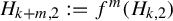 $H_{k+m,2}:=f^m(H_{k,2})$
overlap.
$H_{k+m,2}:=f^m(H_{k,2})$
overlap.
Here,
 $H_{n,0}$
is said to have an order d overlap if there exist
$H_{n,0}$
is said to have an order d overlap if there exist
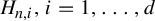 $H_{n,i}, i=1,\ldots ,d$
horizontal cylinders of order n such that for all
$H_{n,i}, i=1,\ldots ,d$
horizontal cylinders of order n such that for all
 $x\in S^1$
and
$x\in S^1$
and
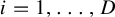 $i=1,\ldots ,D$
,
$i=1,\ldots ,D$
,
 $$ \begin{align*}\widehat H_{n,0}\cap \widehat H_{n,i} \cap \widehat W^s_x \not= \emptyset. \end{align*} $$
Such a family exists for every d and some n. Indeed, suppose we found already
 $H_{n,0}$
having an order
$H_{n,0}$
having an order
 $d-1$
overlap with
$d-1$
overlap with
 $H_{n,i}, i=1,\ldots ,d-1$
. Take
$H_{n,i}, i=1,\ldots ,d-1$
. Take
 $H_{n,d}$
with
$H_{n,d}$
with
 $i^{\prime }_0\not =i_0$
, the zero symbols for
$i^{\prime }_0\not =i_0$
, the zero symbols for
 $H_{n,0}$
and
$H_{n,0}$
and
 $H_{n,d}$
, so that the intersection
$H_{n,d}$
, so that the intersection
 $\widehat H_{n,0}\cap \widehat H_{n,d} \cap \widehat W^s_x $
is non-empty, say contains a point
$\widehat H_{n,0}\cap \widehat H_{n,d} \cap \widehat W^s_x $
is non-empty, say contains a point
 $q=(x,y)$
. Then consider vertical
$q=(x,y)$
. Then consider vertical
 $V_m$
whose
$V_m$
whose
 $\pi _{x,y}$
projection contains q. Then as above, for m large enough,
$\pi _{x,y}$
projection contains q. Then as above, for m large enough,
 $f^m(H_{n,i}), i=0,1,\ldots ,d$
, is the required family. (Notice that the latter intersection contains a point in
$f^m(H_{n,i}), i=0,1,\ldots ,d$
, is the required family. (Notice that the latter intersection contains a point in
 $\widehat \Lambda $
provided
$\widehat \Lambda $
provided
 $q\in \widehat \Lambda $
; however we shall not use this observation.)
$q\in \widehat \Lambda $
; however we shall not use this observation.)
Choose now an arbitrary Birkhoff forward regular
 $\tilde p\in H_{n,0}\cap \Lambda $
. Replace the overlapping cylinders
$\tilde p\in H_{n,0}\cap \Lambda $
. Replace the overlapping cylinders
 $H_{n,i}, i=0,\ldots ,d$
by
$H_{n,i}, i=0,\ldots ,d$
by
 $H_{n+k,i}=f^k(H_{n,i}\cap V_k)$
for
$H_{n+k,i}=f^k(H_{n,i}\cap V_k)$
for
 $V_k\ni p$
and k large, to use time convergences in Birkhoff ergodic theorem. So, for
$V_k\ni p$
and k large, to use time convergences in Birkhoff ergodic theorem. So, for
 $p:=f^k(\tilde p)$
, we have for each
$p:=f^k(\tilde p)$
, we have for each
 $i=0,\ldots ,d$
,
$i=0,\ldots ,d$
,
 $H_{n+k,i}\cap W^s(p) \subset B^s(p,\operatorname {\mathrm {Const}}\unicode{x3bb} ^-_{n+k}( p))$
. This is so due to
$H_{n+k,i}\cap W^s(p) \subset B^s(p,\operatorname {\mathrm {Const}}\unicode{x3bb} ^-_{n+k}( p))$
. This is so due to
 $\chi _\mu (\nu ') < \chi _\mu (\unicode{x3bb} ')$
since then
$\chi _\mu (\nu ') < \chi _\mu (\unicode{x3bb} ')$
since then
 $\nu ^-_k(p) \ll \unicode{x3bb} ^-_{n+k}(p)$
for all k large enough (depending on
$\nu ^-_k(p) \ll \unicode{x3bb} ^-_{n+k}(p)$
for all k large enough (depending on
 $\tilde p$
). Therefore this property is forward invariant under f.
$\tilde p$
). Therefore this property is forward invariant under f.
We conclude that for
 $r=\operatorname {\mathrm {Const}} \unicode{x3bb} ^-_{n+k}(p))$
for
$r=\operatorname {\mathrm {Const}} \unicode{x3bb} ^-_{n+k}(p))$
for
 $x=\pi _x( p)$
, and adequate constant C,
$x=\pi _x( p)$
, and adequate constant C,
 $$ \begin{align} \mu_x^s(B(p,r))\ge C (d+1) r^{t_0}. \end{align} $$
The set
 $A(d)$
of these p has positive measure
$A(d)$
of these p has positive measure
 $\mu $
and is invariant under holonomies
$\mu $
and is invariant under holonomies
 $h_{x,x'}$
. Therefore, invoking also ergodicity of
$h_{x,x'}$
. Therefore, invoking also ergodicity of
 $\mu $
, equation (6.3) holds in every
$\mu $
, equation (6.3) holds in every
 $W^s_x$
for
$W^s_x$
for
 $\mu ^s_x$
-a.e.
$\mu ^s_x$
-a.e.
 $p\in W^s_x$
and
$p\in W^s_x$
and
 $r=r(p,d)$
. If we consider
$r=r(p,d)$
. If we consider
 $A= \bigcap _{d\in \mathbb {N}} ( \bigcup _{n\in \mathbb {N}}f^n( A(d)))$
, then using Frostman lemma, we prove equation (6.1) for
$A= \bigcap _{d\in \mathbb {N}} ( \bigcup _{n\in \mathbb {N}}f^n( A(d)))$
, then using Frostman lemma, we prove equation (6.1) for
 $\Lambda $
replaced by A. Finally, use Lemma 4.3, by which for each x, for
$\Lambda $
replaced by A. Finally, use Lemma 4.3, by which for each x, for
 $A':=\Lambda \setminus A$
,
$A':=\Lambda \setminus A$
,
 $\mu ^s_x (A') =0$
implies
$\mu ^s_x (A') =0$
implies
 $\mathrm {HM}_{t_0}(A')=0$
.
$\mathrm {HM}_{t_0}(A')=0$
.
Similarly, compare the proof of Theorem 4.2, Step 3, one proves equation (6.2).
7 Final remarks
7.1 Large deviations
We refer to the following lemma, see e.g. [Reference Denker, Kesseböhmer, Imkeller and von Storch7, Theorem 1.1].
Lemma 7.1. (On large deviations)
Let
 $F:X\to X$
be an open distance expanding map of a compact metric space, see [Reference Przytycki and Urbański12, §4.1]. Then, for any Hölder continuous potential
$F:X\to X$
be an open distance expanding map of a compact metric space, see [Reference Przytycki and Urbański12, §4.1]. Then, for any Hölder continuous potential
 $\Phi :X \to \mathbb {R}$
, let
$\Phi :X \to \mathbb {R}$
, let
 $\mu _\Phi $
denote the unique Gibbs invariant measure for
$\mu _\Phi $
denote the unique Gibbs invariant measure for
 $\Phi $
, see [Reference Bowen4]. Consider arbitrary Hölder functions
$\Phi $
, see [Reference Bowen4]. Consider arbitrary Hölder functions
 $\phi , \psi : X \to \mathbb {R}$
. Then, for every
$\phi , \psi : X \to \mathbb {R}$
. Then, for every
 $t \in \mathbb {R}$
,
$t \in \mathbb {R}$
,
 $$ \begin{align*}\begin{aligned} &\lim_{n\to\infty}\frac1n \log\mu_\varphi\bigg(\bigg\{x\in X: \mathrm{sgn}(t)S_n \psi(x) \ge \mathrm{sgn}(t) n \int_X\psi\, d\mu_{\varphi+t\psi}\bigg\}\bigg) \\ &\quad= -t\int_X\psi\, d\mu_{\varphi+t\psi}+P_{\mathrm{top}}(\varphi+t\psi)-P_{\mathrm{top}}(\varphi), \end{aligned} \end{align*} $$
where by
 $P_{\mathrm {top}}$
we denote topological pressure, see e.g. [Reference Przytycki and Urbański12].
$P_{\mathrm {top}}$
we denote topological pressure, see e.g. [Reference Przytycki and Urbański12].
Writing
 $\int \psi \, d\mu _{\varphi +t\psi }- \int \psi \, d\mu _{\varphi }:=\varepsilon $
, we can rewrite the above formula as follows:
$\int \psi \, d\mu _{\varphi +t\psi }- \int \psi \, d\mu _{\varphi }:=\varepsilon $
, we can rewrite the above formula as follows:
 $$ \begin{align*}\begin{aligned} &\lim_{n\to\infty}\frac1n \log \mu_\varphi\bigg(\bigg\{x\in X: \, \mathrm{sgn}(t)S_n \psi(x) \ge \mathrm{sgn}(t) n \bigg(\int\psi\, d\mu_{\varphi+t\psi} + \varepsilon\bigg)\bigg\}\bigg) \\ &\quad= -t\int_X\psi\, d\mu_{\varphi+t\psi}+P_{\mathrm{top}}(\varphi+t\psi)-P_{\mathrm{top}}(\varphi) := I(\pm\psi, \varepsilon). \end{aligned} \end{align*} $$
The latter
 $I(\varepsilon )$
measures the nonlinearity of
$I(\varepsilon )$
measures the nonlinearity of
 $t\mapsto P_{\mathrm {top}}(\varphi +t\psi )$
.
$t\mapsto P_{\mathrm {top}}(\varphi +t\psi )$
.
A basic example of such F is
 $\varsigma :\Sigma _d^+\to \Sigma _d^+$
being the left shift map on the one-sided shift space with the standard metric
$\varsigma :\Sigma _d^+\to \Sigma _d^+$
being the left shift map on the one-sided shift space with the standard metric
 $\operatorname {\mathrm {dist}}(\underline i,\underline i')=\sum _{n\in \mathbb {N}}|i_n-i^{\prime }_n|d^{-n}$
.
$\operatorname {\mathrm {dist}}(\underline i,\underline i')=\sum _{n\in \mathbb {N}}|i_n-i^{\prime }_n|d^{-n}$
.
Symmetrically, one considers the right shift map
 $\varsigma ^{-1}:\Sigma ^-_d\to \Sigma ^-_d$
on the space of sequences
$\varsigma ^{-1}:\Sigma ^-_d\to \Sigma ^-_d$
on the space of sequences
 $(\ldots ,i_n,\ldots ,0|)$
. We can consider two-sided sequences or e.g. our solenoid
$(\ldots ,i_n,\ldots ,0|)$
. We can consider two-sided sequences or e.g. our solenoid
 $\Lambda $
identifying sequences with the same future, or past as for our
$\Lambda $
identifying sequences with the same future, or past as for our
 $W^s$
values and
$W^s$
values and
 $f^{-1}$
. Compare Definition 2.1.
$f^{-1}$
. Compare Definition 2.1.
In particular, the following holds.
Lemma 7.2. For every Hölder
 $\phi $
and
$\phi $
and
 $\psi $
, for every
$\psi $
, for every
 $\varepsilon>0$
, there exist
$\varepsilon>0$
, there exist
 $C>0$
and
$C>0$
and
 $\tau>0$
such that for every
$\tau>0$
such that for every
 $n\in \mathbb {N}$
,
$n\in \mathbb {N}$
,
 $$ \begin{align} \mu_\varphi\bigg(\bigg\{x\in X: \bigg|S_n \psi(x) - n\int_{\Sigma_d^+}\psi\,d\mu_\phi\bigg|\ge n\varepsilon\bigg\}\bigg)\le C \exp (-n\tau). \end{align} $$
In §§3 and 4, proving e.g. that
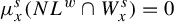 $\mu _x^s(NL^w\cap W^s_x)=0$
in Lemma 3.6, we did not use large deviations. In §5, we already did (the qualitative version of Lemma 7.2. Now we shall show how the usage of large deviations, Lemma 7.1, allows to estimate from above Hausdorff dimension of the set in each
$\mu _x^s(NL^w\cap W^s_x)=0$
in Lemma 3.6, we did not use large deviations. In §5, we already did (the qualitative version of Lemma 7.2. Now we shall show how the usage of large deviations, Lemma 7.1, allows to estimate from above Hausdorff dimension of the set in each
 $W^s_x$
where the holonomy is not locally Lipschitz, thus strengthening Lemma 3.6. See also notation in and after Lemma 2.9.
$W^s_x$
where the holonomy is not locally Lipschitz, thus strengthening Lemma 3.6. See also notation in and after Lemma 2.9.
Proposition 7.3. For every
 $W^s_x$
, the strict inequality
$W^s_x$
, the strict inequality
 $\operatorname {\mathrm {HD}}( NL^w\cap W^s_x) < t_0=\operatorname {\mathrm {HD}}(\Lambda \cap W^s_x)$
holds. More precisely,
$\operatorname {\mathrm {HD}}( NL^w\cap W^s_x) < t_0=\operatorname {\mathrm {HD}}(\Lambda \cap W^s_x)$
holds. More precisely,
 $$ \begin{align} \operatorname{\mathrm{HD}} (NL^w\cap W^s_x) \le \inf_{\varepsilon>0}\max \{A_\varepsilon, B_\varepsilon\}, \end{align} $$
where
 $$ \begin{align*}A_{\varepsilon}= t_0-(I_\varepsilon(\log\unicode{x3bb}',\varepsilon)/\chi_\mu(\unicode{x3bb}'))\bigg/ \bigg(1+\frac{-\chi_\mu(\unicode{x3bb}') - \varepsilon}{\chi_\mu(\eta')-\varepsilon}\bigg) \end{align*} $$
and the same with
 $\log \unicode{x3bb} '$
replaced by
$\log \unicode{x3bb} '$
replaced by
 $-\log \eta '$
. Also, with the latter fraction above replaced by its inverse,
$-\log \eta '$
. Also, with the latter fraction above replaced by its inverse,
 $$ \begin{align*}B_{\varepsilon}=t_0 -\frac{t_0 (1-\varepsilon/\chi_\mu(\unicode{x3bb}') - ({\chi_\mu(\eta') + \varepsilon})/({-\chi_\mu(\unicode{x3bb}')-\varepsilon})) (-\chi_\mu(\unicode{x3bb}')) } {(1+({\chi_\mu(\eta') + \varepsilon})/){-\chi_\mu(\unicode{x3bb}')-\varepsilon})) (-\chi_\mu(\unicode{x3bb}')+\varepsilon)}. \end{align*} $$
Here,
 $A_\varepsilon $
bounds Hausdorff dimension of the irregular part and
$A_\varepsilon $
bounds Hausdorff dimension of the irregular part and
 $B_\varepsilon $
bounds Hausdorff dimension of the regular non-Lipschitz part.
$B_\varepsilon $
bounds Hausdorff dimension of the regular non-Lipschitz part.
For
 $\varepsilon \approx 0$
, the number
$\varepsilon \approx 0$
, the number
 $A_\varepsilon $
is bigger. On the other end, for
$A_\varepsilon $
is bigger. On the other end, for
 $({\chi _\mu (\eta ') + \varepsilon })/({-\chi _\mu (\unicode{x3bb} ')-\varepsilon })$
almost 1, the number
$({\chi _\mu (\eta ') + \varepsilon })/({-\chi _\mu (\unicode{x3bb} ')-\varepsilon })$
almost 1, the number
 $B_\varepsilon $
dominates. Optimum is in between.
$B_\varepsilon $
dominates. Optimum is in between.
Proof First we prove the estimate (7.2) for
 $B_\varepsilon $
. We rely on §5, the proof of Theorem 5.1, Step 1. The coefficient
$B_\varepsilon $
. We rely on §5, the proof of Theorem 5.1, Step 1. The coefficient
 $\alpha $
is not needed, since
$\alpha $
is not needed, since
 $NL^w$
is a local property and overlappings of remote cylinders do not count (see the proof of Theorem 5.1, Step 3).
$NL^w$
is a local property and overlappings of remote cylinders do not count (see the proof of Theorem 5.1, Step 3).
We obtain the uniform estimate for every
 $(\unicode{x3bb} ,\varepsilon ,m)$
-backward regular
$(\unicode{x3bb} ,\varepsilon ,m)$
-backward regular
 $H_m$
, with n satisfying equation (5.3) Its ‘contaminated part’ can be estimated as follows, see equations (5.4) and (4.10),
$H_m$
, with n satisfying equation (5.3) Its ‘contaminated part’ can be estimated as follows, see equations (5.4) and (4.10),
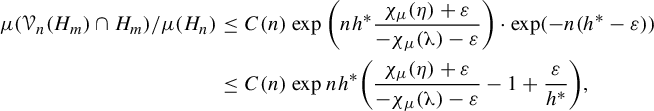
where
 $C(n)$
grows sub-exponentially. We used here, as already e.g. in equation (5.4), the fact that
$C(n)$
grows sub-exponentially. We used here, as already e.g. in equation (5.4), the fact that
 $\operatorname {\mathrm {Const}}^{-1}\mu (H_m \cap V_n)/ \mu (H_m) \mu (V_n) <\operatorname {\mathrm {Const}}$
following from Gibbs property of
$\operatorname {\mathrm {Const}}^{-1}\mu (H_m \cap V_n)/ \mu (H_m) \mu (V_n) <\operatorname {\mathrm {Const}}$
following from Gibbs property of
 $\mu $
.
$\mu $
.
Now by summing over regular
 $H_m$
with weights
$H_m$
with weights
 $\mu (H_m)$
, we get the same estimate for
$\mu (H_m)$
, we get the same estimate for
![]() and by the f-invariance of
and by the f-invariance of
 $\mu $
, the same estimate for
$\mu $
, the same estimate for
![]() for
for
 $n=n(\varepsilon ,m)$
, built of cylinders
$n=n(\varepsilon ,m)$
, built of cylinders
 $H_{m+n}$
.
$H_{m+n}$
.
Now we shall translate the measure estimate above for all
 $m, n(\varepsilon ,m)$
, to an estimate of Hausdorff dimension.
$m, n(\varepsilon ,m)$
, to an estimate of Hausdorff dimension.
Denote
 $\mu (\textbf {H}'(n))$
by
$\mu (\textbf {H}'(n))$
by
 $\overline \mu _n$
. By Gibbs property of
$\overline \mu _n$
. By Gibbs property of
 $\mu =\mu _{t_0}$
and using normalized restrictions
$\mu =\mu _{t_0}$
and using normalized restrictions
 $\mu _n:=\mu |_{\textbf {H}'(n)}/\overline \mu _n$
, considering conditional measures on
$\mu _n:=\mu |_{\textbf {H}'(n)}/\overline \mu _n$
, considering conditional measures on
 $W^s$
(not changing notation), we get for each
$W^s$
(not changing notation), we get for each
 $H_{n+m}\subset \textbf {H}'(n)$
and p in it,
$H_{n+m}\subset \textbf {H}'(n)$
and p in it,
where
 $\vartheta _n:={\log \overline \mu _n}/({(n+m)(\chi _\mu (\unicode{x3bb} ')-\varepsilon )})$
, with m expressed by n maximal possible to satisfy equation (5.3). So, for any
$\vartheta _n:={\log \overline \mu _n}/({(n+m)(\chi _\mu (\unicode{x3bb} ')-\varepsilon )})$
, with m expressed by n maximal possible to satisfy equation (5.3). So, for any
 $x\in S^1$
,
$x\in S^1$
,
 $$ \begin{align} \sum_{H_{n+m}\subset\textbf{H}'(n)} \operatorname{\mathrm{diam}} (H_{n+m} \cap W^s_x)^{(t_0-\vartheta_n)\kappa} \le \sum_{H_{n+m}\subset\textbf{H}'(n)} \mu_n (H_{n+m})=1, \end{align} $$
where
 $\kappa =({\chi _\mu (\unicode{x3bb} ') -e})/{\chi _\mu (\unicode{x3bb} ')}$
. By an arbitrarily small change of
$\kappa =({\chi _\mu (\unicode{x3bb} ') -e})/{\chi _\mu (\unicode{x3bb} ')}$
. By an arbitrarily small change of
 $\kappa $
, we can assure the bound by 1 replaced by numbers tending exponentially to 0 as
$\kappa $
, we can assure the bound by 1 replaced by numbers tending exponentially to 0 as
 $m\to \infty $
, allowing summing over m.
$m\to \infty $
, allowing summing over m.
So, taking
 $\varepsilon \to 0$
, for
$\varepsilon \to 0$
, for
 $\vartheta :=\liminf _{n\to \infty }\vartheta _n$
,
$\vartheta :=\liminf _{n\to \infty }\vartheta _n$
,
 $$ \begin{align*}\operatorname{\mathrm{HD}}(NL^w\cap W^s_x) \le \operatorname{\mathrm{HD}}\Big(\limsup_{n\to\infty} \textbf{H}'(n)\Big) \le \vartheta. \end{align*} $$
This, after simple calculations, yields the estimate by
 $B_\varepsilon $
in our Proposition. For an explanation of the structure of
$B_\varepsilon $
in our Proposition. For an explanation of the structure of
 $L^s$
complementary to the set
$L^s$
complementary to the set
 $NL^w \subset \limsup _{n\to \infty } \textbf {H}'(n)$
, (with
$NL^w \subset \limsup _{n\to \infty } \textbf {H}'(n)$
, (with
 $2n$
there in place of
$2n$
there in place of
 $m+n$
here), see Remark 5.3.
$m+n$
here), see Remark 5.3.
Now we estimate the irregular (backward) part, related to
 $A_\varepsilon $
. For this, we define similarly to
$A_\varepsilon $
. For this, we define similarly to
 $\textbf {H}_i$
in §5 but with
$\textbf {H}_i$
in §5 but with
 $k=0$
and
$k=0$
and
 $\alpha =1$
. We add
$\alpha =1$
. We add
 $\unicode{x3bb} ,\eta $
and
$\unicode{x3bb} ,\eta $
and
 $\varepsilon $
in the notation of
$\varepsilon $
in the notation of
 $\textbf {H}_i$
. We consider
$\textbf {H}_i$
. We consider
 $$ \begin{align*}\textbf{H}_1(\unicode{x3bb},\varepsilon,m, \operatorname{\mathrm{irreg}})\subset \bigcup H_{m+n}\end{align*} $$
and
 $$ \begin{align*}\textbf{H}_2(\eta,\varepsilon,n, \operatorname{\mathrm{irreg}})\subset \bigcup H_{m+n}.\end{align*} $$
We define also as in the proof of Theorem 5.1, Step 3, the set
 $$ \begin{align*}\textbf{H}_3(\xi,\varepsilon, n, \operatorname{\mathrm{irreg}})\subset \bigcup H_{m+n} \quad\text{ for }\xi=\unicode{x3bb},\nu.\end{align*} $$
Applying Lemma 7.1 for
 $\psi =\log \unicode{x3bb} '$
, replacing m by
$\psi =\log \unicode{x3bb} '$
, replacing m by
 $n+m$
, we get for
$n+m$
, we get for
 $\textbf {H}_1$
,
$\textbf {H}_1$
,
 $$ \begin{align*}\operatorname{\mathrm{HD}} (\limsup \textbf{H}_1(\unicode{x3bb},\varepsilon,m, \operatorname{\mathrm{irreg}})) \le t_0 - (I(\log\unicode{x3bb}',\varepsilon)/\chi_\mu(\unicode{x3bb}')) \bigg/ \bigg(1+\frac{-\chi_\mu(\unicode{x3bb}')-\varepsilon}{\chi_\mu(\eta') + \varepsilon}\bigg), \end{align*} $$
for
 $\textbf {H}_2$
, replacing n by
$\textbf {H}_2$
, replacing n by
 $n+m$
,
$n+m$
,
 $$ \begin{align*}\operatorname{\mathrm{HD}} (\limsup \textbf{H}_2(\eta,\varepsilon,n, \operatorname{\mathrm{irreg}})) \le t_0 - (I(-\log\eta',\varepsilon)/\chi_\mu(\unicode{x3bb}')) \bigg/ \bigg(1+\frac{\chi_\mu(\eta') + \varepsilon}{-\chi_\mu(\unicode{x3bb}')-\varepsilon}\bigg) \end{align*} $$
and for
 $\textbf {H}_3$
,
$\textbf {H}_3$
,
 $$ \begin{align*}\kern-10pt\operatorname{\mathrm{HD}} (\limsup \textbf{H}_3(\unicode{x3bb},\varepsilon, n, \operatorname{\mathrm{irreg}})) \le t_0 - (I(\log\unicode{x3bb}',\varepsilon)/\chi_\mu(\unicode{x3bb}')) \bigg/ \bigg(1+\frac{\chi_\mu(\eta') + \varepsilon}{-\chi_\mu(\unicode{x3bb}')-\varepsilon}\bigg).\\[-43pt] \end{align*} $$
7.2 Generalization to one-dimensional expanding attractors
All the theorems in this paper hold also for hyperbolic expanding attractors in dimension 3 with one-dimensional unstable manifolds, non-uniformly thin (see definition in §1) and satisfying the transversality assumption, of which our solenoids are examples. The only exception is the Theorem 6.1 on singularity of Hausdorff measures, where the assumption that for some
 $p,q\in \Lambda $
, a non-empty intersection of projections
$p,q\in \Lambda $
, a non-empty intersection of projections
 $\widehat W^u(p)$
and
$\widehat W^u(p)$
and
 $\widehat W^u(q)$
is needed. For our solenoids, it holds automatically, but for extensions to
$\widehat W^u(q)$
is needed. For our solenoids, it holds automatically, but for extensions to
 $\mathbb {R}^3$
of say Plykin or DA attractor, it is not so. See [Reference Robinson18].
$\mathbb {R}^3$
of say Plykin or DA attractor, it is not so. See [Reference Robinson18].
Proofs are the same since these attractors are extensions of expanding maps on branched 1-manifolds and Markov coding can be used.
7.3 More on solenoids—coordinates
In fact, Theorems 1.2–1.6 hold for
 $$ \begin{align} f(x,y,z):= (\eta(x,y,z), \unicode{x3bb}(x,y,z) + u(x), \nu(x,y,z ) + v(x)), \end{align} $$
of class
 $C^{1+\varepsilon }$
, injective, such that
$C^{1+\varepsilon }$
, injective, such that
 $f(\operatorname {\mathrm {cl}} M)\subset M$
, satisfying
$f(\operatorname {\mathrm {cl}} M)\subset M$
, satisfying
 $\unicode{x3bb} (x,0,0)=\nu (x,0,0)=0$
, with hyperbolic attractor
$\unicode{x3bb} (x,0,0)=\nu (x,0,0)=0$
, with hyperbolic attractor
 $\Lambda $
, and satisfying transversality, the non-conformal form more general than f in the triangular in equation (1.1).
$\Lambda $
, and satisfying transversality, the non-conformal form more general than f in the triangular in equation (1.1).
Indeed, we are interested in a non-conformal solenoid, so we assume that the tangent bundle on M, or at least on
 $\Lambda $
, splits into
$\Lambda $
, splits into
 $T_\Lambda M=E^u \oplus E^{s}$
,
$T_\Lambda M=E^u \oplus E^{s}$
,
 $Df$
invariant, where
$Df$
invariant, where
 $E^s$
, the stable one, splits further into weak stable and strong stable
$E^s$
, the stable one, splits further into weak stable and strong stable
 $T_\Lambda M= E^u \oplus E^{ws} \oplus E^{ss}$
, or at least
$T_\Lambda M= E^u \oplus E^{ws} \oplus E^{ss}$
, or at least
 $E^s$
contains a strong stable
$E^s$
contains a strong stable
 $E^{ss}$
. Note that
$E^{ss}$
. Note that
 $E^s$
is dynamically defined on the whole M, not only on
$E^s$
is dynamically defined on the whole M, not only on
 $\Lambda $
, by
$\Lambda $
, by
 $E^s(p):=\lim Df^{-n} (C^s(f^n(p)))$
, where
$E^s(p):=\lim Df^{-n} (C^s(f^n(p)))$
, where
 $C^s$
denotes a stable cone taken equal to a cone at a point in
$C^s$
denotes a stable cone taken equal to a cone at a point in
 $\Lambda $
near
$\Lambda $
near
 $f^n(p)$
. Similarly, one proves that the bundle
$f^n(p)$
. Similarly, one proves that the bundle
 $E^s$
on M is integrable to a stable foliation
$E^s$
on M is integrable to a stable foliation
![]() of M. As having codimension one, it is
of M. As having codimension one, it is
 $C^{1+\varepsilon }$
, see [Reference Pinto, Rand and Ferreira11]. Therefore, under an appropriate
$C^{1+\varepsilon }$
, see [Reference Pinto, Rand and Ferreira11]. Therefore, under an appropriate
 $C^{1+\varepsilon }$
change of coordinates, it becomes the foliation of M by vertical discs
$C^{1+\varepsilon }$
change of coordinates, it becomes the foliation of M by vertical discs
 $W^s_x=\{x\}\times \mathbb {D}$
.
$W^s_x=\{x\}\times \mathbb {D}$
.
Additionally, strong stable foliation
![]() (of the whole M as obtained as a limit from the future) can be made consisting of vertical intervals, that is, with
(of the whole M as obtained as a limit from the future) can be made consisting of vertical intervals, that is, with
 $x,y$
constant. This foliation is known to be
$x,y$
constant. This foliation is known to be
 $C^{1+\varepsilon }$
in
$C^{1+\varepsilon }$
in
![]() , see [Reference Brown5], so, after a change of coordinates so that it becomes vertical, our diffeomorphism is
, see [Reference Brown5], so, after a change of coordinates so that it becomes vertical, our diffeomorphism is
 $C^{1+\varepsilon }$
in each
$C^{1+\varepsilon }$
in each
 $W^s$
. However, we do not know what is the smoothness of f in the new coordinates in the whole M.
$W^s$
. However, we do not know what is the smoothness of f in the new coordinates in the whole M.
Therefore, to deduce this general case from our triangular case by change of coordinates, we just assume
![]() is
is
 $C^{1+\varepsilon }$
in M. A question stays open whether this assumption is needed, that is, whether we really use f being
$C^{1+\varepsilon }$
in M. A question stays open whether this assumption is needed, that is, whether we really use f being
 $C^{1+\varepsilon }$
in the triangular coordinates.
$C^{1+\varepsilon }$
in the triangular coordinates.
The following completes the topological picture. Suppose f is already in the triangular form.
Lemma 7.4. There exists on M a change of coordinates
 $\Psi (x,y,z)=(x,y,\psi (y,z)$
, bi-Lipschitz continuous, such that the foliation into the sets
$\Psi (x,y,z)=(x,y,\psi (y,z)$
, bi-Lipschitz continuous, such that the foliation into the sets
 $x,z$
constant is invariant and its
$x,z$
constant is invariant and its
 $\Psi ^{-1}$
-image is a central stable foliation
$\Psi ^{-1}$
-image is a central stable foliation
![]() with leaves
with leaves
 $C^1$
smooth.
$C^1$
smooth.
Proof Extend f to
 $\tilde f :S^1 \times \mathbb {R}^2\to S^1 \times \mathbb {R}^2$
so that
$\tilde f :S^1 \times \mathbb {R}^2\to S^1 \times \mathbb {R}^2$
so that
 $\unicode{x3bb} $
and
$\unicode{x3bb} $
and
 $\nu $
are linear with respect to y and z, respectively, far from M.
$\nu $
are linear with respect to y and z, respectively, far from M.
Next find
![]() as a limit of
as a limit of
![]() , where
, where
![]() is the foliation of M into the intervals
is the foliation of M into the intervals
 $x,z$
constant. By bounded distortion, one gets Lipschitz property of the limit and, in particular, a true foliation (leaves do no glue partially to each other in the limit).
$x,z$
constant. By bounded distortion, one gets Lipschitz property of the limit and, in particular, a true foliation (leaves do no glue partially to each other in the limit).
Our
 $Df$
in these coordinates would be diagonal which would ease estimates. Unfortunately, this central stable foliation and, therefore, f in the new coordinates seems usually not
$Df$
in these coordinates would be diagonal which would ease estimates. Unfortunately, this central stable foliation and, therefore, f in the new coordinates seems usually not
 $C^{1+\varepsilon }$
.
$C^{1+\varepsilon }$
.
7.4 Summary of our strategies
The key objects in the paper are ‘rectangles’ being intersection of horizontal and vertical strips
 $\widehat H_m$
and
$\widehat H_m$
and
 $\widehat V_n$
, ‘cylinders’ of level m and n, projections to the plane
$\widehat V_n$
, ‘cylinders’ of level m and n, projections to the plane
 $(x,y)$
of tubes and thickened discs. Such Markov rectangles are basic objects in hyperbolic dynamics.
$(x,y)$
of tubes and thickened discs. Such Markov rectangles are basic objects in hyperbolic dynamics.
Horizontal strips can intersect transversally other horizontal strips. An issue is to estimate how the large part of any horizontal strip is intersected, ‘contaminated’ by other horizontal strips, measured in a number of contaminated (with margins) rectangles. The tool is going backward by
 $f^{-m}$
or forward by
$f^{-m}$
or forward by
 $f^n$
to large scale, so that the rectangles become full (that is, over
$f^n$
to large scale, so that the rectangles become full (that is, over
 $[0,2\pi ]$
) horizontal strips and results do not depend on sections by stable discs
$[0,2\pi ]$
) horizontal strips and results do not depend on sections by stable discs
 $W^s$
. We distinguish Birkhoff irregular sets among full unstable manifolds (over
$W^s$
. We distinguish Birkhoff irregular sets among full unstable manifolds (over
 $[0,2\pi ]$
) and prove they have stable SRB-measure 0 and even Hausdorff dimension in each
$[0,2\pi ]$
) and prove they have stable SRB-measure 0 and even Hausdorff dimension in each
 $W^s$
less than the dimension of
$W^s$
less than the dimension of
 $\Lambda \cap W^s$
. We estimate also the size of the contaminated set of Birkhoff regular unstable manifolds. In each section, the choice of m to n (or vice versa) and auxiliary k is different, depending on our needs.
$\Lambda \cap W^s$
. We estimate also the size of the contaminated set of Birkhoff regular unstable manifolds. In each section, the choice of m to n (or vice versa) and auxiliary k is different, depending on our needs.
Acknowledgements
We wish to thank Adam Abrams for making the pictures for this paper. We are grateful to Aaron Brown and Jörg Schmeling for useful discussions. All the authors are partially supported by Polish NCN grant 2019/33/B/ST1/00275.


 Open access