Refinements of Katz–Sarnak theory for the number of points on curves over finite fields

Abstract

This paper goes beyond Katz–Sarnak theory on the distribution of curves over finite fields according to their number of rational points, theoretically, experimentally, and conjecturally. In particular, we give a formula for the limits of the moments measuring the asymmetry of this distribution for (non-hyperelliptic) curves of genus $g\geq 3$. The experiments point to a stronger notion of convergence than the one provided by the Katz–Sarnak framework for all curves of genus $\geq 3$. However, for elliptic curves and for hyperelliptic curves of every genus, we prove that this stronger convergence cannot occur.

1 Introduction

Katz–Sarnak theory [KS99] gives a striking unified framework to understand the distribution of the traces of Frobenius for a family of curves ¹ of genus g over a finite field $\mathbb {F}_q$ when q goes to infinity. It has been used in many specific cases (see [AS10, BCD⁺18, CDSS17, FKRS12, HKL⁺20, KS09, Vlă01] among others). Although powerful, this theory can neither in general predict the number of curves over a given finite field with a given trace, nor distinguish between the family of all curves and the family of hyperelliptic curves when $g\geq 3$ . This paper can be seen as an attempt to go beyond Katz–Sarnak results, theoretically, experimentally, and conjecturally. We hope that this blend will excite the curiosity of the community.

We begin by resuming our study of sums of powers of traces initiated in [BHLGR23]. If $C/\mathbb {F}_q$ is a curve of genus g, we denote by $[C]$ the set of representatives of its twists and define

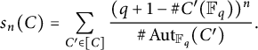$$\begin{align*}s_n(C) = \sum_{C' \in [C]} \frac{(q+1-\#C'(\mathbb{F}_q))^n}{\# \operatorname{\mathrm{Aut}}_{\mathbb{F}_q}(C')}. \end{align*}$$

As shown in [BHLGR23, Proposition 3.1], the $s_n(C)$ are integers and we denote by $S_{n}(q,\mathcal {X})$ the sum of the $s_n(C)$ when C runs over a set of representatives for the $\overline {\mathbb {F}}_q$ -isomorphism classes of curves C over $\mathbb {F}_q$ in $\mathcal {X}$ , where $\mathcal {X}$ can be, for example,

• • the moduli space $\mathcal {M}_{1,1}$ of elliptic curves,

• • the moduli space $\mathcal {M}_g$ of curves of genus $g>1$ ,

• • the moduli space $\mathcal {H}_g$ of hyperelliptic curves of genus $g>1$ , or

• • the moduli space $\mathcal {M}^{\text {nhyp}}_g$ of non-hyperelliptic curves of genus $g>2$ .

In Remark 2.2, we will briefly recall that $S_n(q,\mathcal {M}_{1,1})$ can be determined for all q and n in terms of traces of Hecke operators on spaces of elliptic modular cusp forms. For every q and n, we can also find expressions for $S_n(q,\mathcal {M}_2)=S_n(q,\mathcal {H}_2)$ in terms of traces of Hecke operators acting on spaces of Siegel modular cusp forms of genus $2$ (and genus $1$ ) starting from [Pet15, Theorem 2.1] (see [BF22, Section 4.5] for a few more details). For every $g \geq 3$ , there are known explicit formulae for $S_n(q,\mathcal {X})$ only for the first values of n (see, for instance, [BHLGR23, Theorem 3.4] for $\mathcal {H}_g$ (note that the odd n values are equal to $0$ in this case) and [Ber08] for $\mathcal {M}^{\text {nhyp}}_3$ ). However, it is possible to give an interpretation for

with $\mathcal {X}=\mathcal {M}_g$ , $\mathcal {H}_g$ , or $\mathcal {M}^{\text {nhyp}}_g$ for every $g \geq 2$ and even $n \geq 2$ in terms of representation theory of the compact symplectic group $\operatorname {\mathrm {USp}}_{2g}$ . This is achieved in [BHLGR23, Theorem 3.8] using the ideas of Katz and Sarnak.

Our first contributions are gathered in Theorem 2.1. Using the results of Johnson [Joh83] and Hain [Hai95], together with results of Petersen [Pet15, Pet16] about the first cohomology group of symplectic local systems on $\mathcal {M}_g$ , we can prove that for even values of $n>0$ , we have

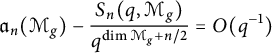(1.1) $$ \begin{align} \mathfrak{a}_n(\mathcal{M}_g) - \frac{S_n(q,\mathcal{M}_g)}{q^{\dim \mathcal{M}_g+n/2}} = O(q^{-1}) \end{align} $$

when $g\geq 2$ , whereas Katz–Sarnak would only give $O(q^{-1/2})$ . Since $\mathfrak {a}_n(\mathcal {M}_g)=0$ for odd values of n, this suggests replacing the exponent in the power of q in the denominator of the expression defining $\mathfrak {a}_n(\mathcal {M}_g)$ with a smaller number. As far as we know, this has not been considered previously. We therefore introduce for odd n

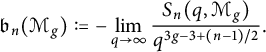
Theorem 2.1 gives $\mathfrak {b}_n(\mathcal {M}_g)$ in terms of an explicit integral and in terms of the representation theory of $\operatorname {\mathrm {USp}}_{2g}$ . This second description makes it easy to compute. The idea to use information about the cohomology of moduli space of curves to predict the number of curves over a given finite field with a given trace can also be found in [AEK⁺15], but there g goes to infinity.

The deep relations between the sum of traces and Katz–Sarnak theory become clearer once we switch to a probabilistic point of view. In Section 3, we introduce the classical probability measure $\mu _{q,g}$ on the interval $[-2g,2g]$ derived from the numbers of $\mathbb {F}_q$ -isomorphism classes of curves of genus $g>1$ with given traces of Frobenius. From Katz–Sarnak, we then know that the sequence of measures $(\mu _{q,g})$ weakly converges to a continuous measure $\mu _g$ with an explicit density ${\mathfrak {f}}_g$ (see [Bil95, Theorem 2.1] for equivalent definitions of weak convergence of measures). In this language, the numbers $\mathfrak {a}_n(\mathcal {M}_g)$ can be understood as the nth moments of the measure $\mu _g$ , and we can refine Katz–Sarnak theory using a second continuous function ${\mathfrak {h}}_g$ whose nth moments are the numbers $\mathfrak {b}_n(\mathcal {M}_g)$ (see Theorem 3.1).

In Section 4, we investigate whether the Katz–Sarnak limiting distributions can be used to approximate the number of curves over a given finite field $\mathbb {F}_q$ of a given genus and with a given trace of Frobenius; one might hope that integrating that distribution over an interval of length $1/\sqrt {q}$ around $t/\sqrt {q}$ would give a value close to the number of genus-g curves over $\mathbb {F}_q$ having trace t. We show that this does not happen for elliptic curves or for hyperelliptic curves of any genus. For elliptic curves, Proposition 4.5 shows that the number of elliptic curves with a given trace can be an arbitrarily large multiple of this naïve Katz–Sarnak prediction (see also Figure 3). For hyperelliptic curves, Proposition 4.2 shows (roughly speaking) that if the number of curves is asymptotically bounded above and below by two multiples of the naïve Katz–Sarnak prediction, then the ratio of these two multiples is bounded below by a fixed number strictly greater than $1$ (see Figure 1).

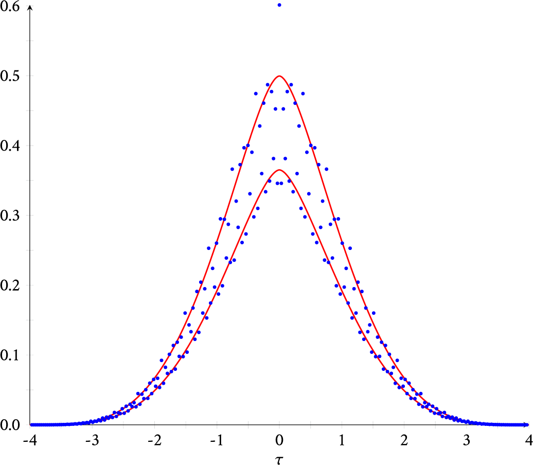
Figure 1: Data for curves of genus $2$ over $\mathbb {F}_q$ for $q=1,009$ . The blue dots are the points $(t/\sqrt {q},\sqrt {q}\,\mathcal {N}^{\text {hyp}}_{q,2}(t/\sqrt {q}))$ for integers $t\in [-126,126]$ . The red curves are the functions $b {\mathfrak {f}}_2(\tau )$ and $c {\mathfrak {f}}_2(\tau )$ , where $b=38/45$ and $c=52/45$ are the bounds given by Proposition 4.2 for $g=2$ when $\varepsilon = 0$ .

Figure 2: Scaled data for curves of genus $2$ over $\mathbb {F}_q$ for $q=1,009$ . The blue dots are the points $(t/\sqrt {q},s\sqrt {q}\, \mathcal {N}^{\text {hyp}}_{q,2}(t/\sqrt {q}))$ for integers $t\in [-126,126]$ , where $s=45/52$ if t is even and $s=45/38$ if t is odd. The red curve is the function ${\mathfrak {f}}_2(\tau )$ .

On the other hand, numerical experiments suggest that the elliptic and hyperelliptic cases differ in the sense that it is easy to “correct” the distribution in the hyperelliptic cases to observe a good approximation by the density function ${\mathfrak {f}}_g$ (see Figure 2). Even stronger, computations for all non-hyperelliptic curves of genus $3$ (see Figure 4) make us dream that the naïve Katz–Sarnak approximation does directly give an accurate estimate for the number of curves with a given number of points. This leads us to claim the bold Conjecture 5.1. The heuristic idea behind this conjecture is that for each trace, one is averaging over many isogeny classes which somehow would allow this stronger convergence as long as there are no obvious arithmetic obstructions. Our attempts to use the better convergence rates of the moments in the case of $\mathcal {M}_g$ for $g \geq 3$ to prove this conjecture were unfortunately unsuccessful. However, for $g=1$ , we would like to point out the shortening of the intervals of convergence obtained in [Ma23], which may give some hints for addressing the question.

Finally, in Section 5, we revisit the work of [LRR⁺19] on the symmetry breaking for the trace distribution of (non-hyperelliptic) genus $3$ curves, by looking at the difference between the number of curves with trace t and the number of curves with trace $-t$ . In probabilistic terms, this asymmetry is given by a signed measure $\nu _{q,g}$ . Although this signed measure weakly converges to $0$ when q goes to infinity, by Corollary 5.3, the moments of $\sqrt {q} \,\nu _{q,g}$ converge to $-2 \mathfrak {b}_n(\mathcal {M}_g)$ when n is odd (and are trivially $0$ when n is even). In particular, this shows that by “zooming in” on the Katz–Sarnak distribution, one can spot a difference between the behavior for hyperelliptic curves (for which the corresponding signed measures would all be $0$ ) and for non-hyperelliptic curves.

In the same spirit as Section 4, the experimental data for $g=3$ (see Figure 5) and the convergence of moments lead us to conjecture that the sequence of signed measures $(\sqrt {q} \,\nu _{q,g})$ weakly converges to the continuous signed measure with density $-2 {\mathfrak {h}}_g$ for all $g \geq 3$ . Notice that in contrast to the case of positive bounded measures, the convergence of moments of signed measures on a compact interval does not directly imply weak convergence (see Example 5.4).

With such a conjecture in hand, one may then improve on the result of [LRR⁺19] that heuristically approximated the limit density of $(\sqrt {q} \,\nu _{q,g})$ by the function

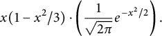$$ \begin{align*}x (1-x^2/3) \cdot \left(\frac{1}{\sqrt{2\pi}} e^{-x^2 / 2}\right).\end{align*} $$

Using the first values of $\mathfrak {b}_n(\mathcal {M}_3)$ , we get the better approximation

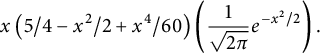$$\begin{align*}x \left(5/4- x^2/2+ x^4/60\right) \left(\frac{1}{\sqrt{2 \pi}} e^{-x^2/2}\right). \end{align*}$$

2 Limits of sums of powers of traces

Fix a prime power q. Let us start by recalling some definitions and results from [BHLGR23].

Definition 2.1 Let $\mathcal {X}=\mathcal {H}_g$ , $\mathcal {M}_g$ or $\mathcal {M}^{\text {nhyp}}_g$ for any $g \geq 2$ , or $\mathcal {X}=\mathcal {M}_{1,1}$ .

• ⋆ Recall from Section 1 that one defines

  $$\begin{align*}S_n(q,\mathcal{X})=\sum_{[C] \in \mathcal{X}(\mathbb{F}_q)} \sum_{C' \in [C]} \frac{(q+1-\#C'(\mathbb{F}_q))^n}{\# \operatorname{\mathrm{Aut}}_{\mathbb{F}_q}(C')}, \end{align*}$$
  where $[C]$ is a point of $\mathcal {X}(\mathbb {F}_q)$ representing the $\overline {\mathbb {F}}_q$ -isomorphism class of a curve $C/\mathbb {F}_q$ , and the second sum spans the set of representatives of all twists $C'$ of C.

• ⋆ For every $n \geq 1$ , let

  
  with $\mathcal {X}=\mathcal {H}_g$ or $\mathcal {M}_g$ or $\mathcal {M}^{\text {nhyp}}_g$ for any $g \geq 2$ , or with $\mathcal {X}=\mathcal {M}_{1,1}$ .

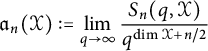
Define and

and recall from [BHLGR23, Theorem 2.1] that for every $g \geq 2$ and $n \geq 1$ ,

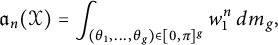$$\begin{align*}\mathfrak{a}_n(\mathcal{X})= \int_{{(\theta_1,\ldots,\theta_g)}\in [0,\pi]^g } w_1^n \, d m_g, \end{align*}$$

with $\mathcal {X}=\mathcal {H}_g$ or $\mathcal {M}_g$ or $\mathcal {M}^{\text {nhyp}}_g$ . Notice that for a fixed value of g, $\mathfrak {a}_n(\mathcal {X})$ does not depend on $\mathcal {X}$ , and $\mathfrak {a}_n(\mathcal {X})=0$ for odd n.

In order to go deeper in the limit distribution, we will also look at the “next term” of the limit of $\frac {S_n(q,\mathcal {X})}{q^{\dim \mathcal {X}+n/2}}$ when $\mathcal {X}=\mathcal {M}_g$ .

Definition 2.2 For every $g \geq 2$ and $n \geq 1$ , let

To state our results, we need to recall basic facts about the representations of $\operatorname {\mathrm {USp}}_{2g}$ with coefficients in $\mathbb {Q}_{\ell }$ , where $\ell $ is a prime distinct from the characteristic of $\mathbb {F}_q$ . The irreducible representations $V_{\lambda }$ of $\operatorname {\mathrm {USp}}_{2g}$ are indexed by the highest weight $\lambda =(\lambda _1,\ldots ,\lambda _g)$ with $\lambda _1 \geq \cdots \geq \lambda _g \geq 0$ . The corresponding characters $\chi _{\lambda }$ are the symplectic Schur polynomials $\mathbf {s}_{\langle \lambda \rangle }(x_1,\ldots ,x_g) \in \mathbb {Z}[x_1,\ldots ,x_g,x_1^{-1},\ldots ,x_g^{-1}]$ in the sense that if $A \in \operatorname {\mathrm {USp}}_{2g}$ has eigenvalues $\alpha _1,\ldots ,\alpha _g,\alpha _1^{-1},\ldots ,\alpha _g^{-1}$ , then $\chi _{\lambda }(A)=\mathbf {s}_{\langle \lambda \rangle }(\alpha _1,\ldots ,\alpha _g)$ (see [FH91, Proposition 24.22 and (A.45)]). In the notation, we will suppress the $\lambda _j$ that are $0$ . Put $\lvert \lambda \rvert =\lambda _1+\cdots +\lambda _g$ and note that $V_{\lambda }^{\vee } \cong V_{\lambda }$ .

Theorem 2.1 Let $V=V_{(1)}$ denote the standard representation.

1. (1) Let $\mathcal {X}=\mathcal {H}_g$ , $\mathcal {M}_g$ , $\mathcal {M}^{\text {nhyp}}_g$ for any $g \geq 2$ , or $\mathcal {M}_{1,1}$ . For every $n \geq 1$ , $\mathfrak {a}_n(\mathcal {X})$ is equal to the number of times the trivial representation appears in the $\operatorname {\mathrm {USp}}_{2g}$ -representation $V^{\otimes n}$ . ²

2. (2) For every $g \geq 3$ and $n \geq 1$ , $\mathfrak {b}_n(\mathcal {M}_g)$ is equal to the number of times the representation $V_{(1,1,1)}$ appears in the $\operatorname {\mathrm {USp}}_{2g}$ -representation $V^{\otimes n}$ . In particular, $\mathfrak {b}_n(\mathcal {M}_g)=0$ for n even.

3. (3) For every $n \geq 1$ , $\mathfrak {b}_n(\mathcal {M}_2)=0$ .

4. (4) For every $g \geq 2$ and $n \geq 1$ ,

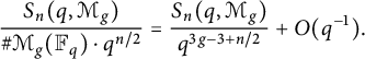
   $$\begin{align*}\mathfrak{a}_n(\mathcal{M}_g)-\frac{\mathfrak{b}_n(\mathcal{M}_g)}{\sqrt{q}}= \frac{S_n(q,\mathcal{M}_g)}{q^{3g-3+n/2}} +O(q^{-1}). \end{align*}$$

5. (5) For every $g \geq 3$ and $n \geq 1$ , we have

   (2.1) $$ \begin{align} \mathfrak{b}_n(\mathcal{M}_g)= \int_{{(\theta_1,\ldots,\theta_g)}\in [0,\pi]^g } w_1^n \Bigg(\frac{1}{6}w_1^3-\frac{1}{2}w_1w_2+\frac{1}{3}w_3-w_1 \Bigg) \, d m_g. \end{align} $$

Proof Poincaré duality gives a symplectic pairing on the first $\ell $ -adic étale cohomology group of a curve. We will be interested in the action of Frobenius on these cohomology groups, and since we need to take the size of the eigenvalues of Frobenius into account, we will consider representations of $\operatorname {\mathrm {GSp}}_{2g}$ . Let $\mathbb {Q}_{\ell }(-1)$ denote the multiplier representation or similitude character; if we identify $\operatorname {\mathrm {GSp}}_{2g}$ as the group of automorphisms of a $2g$ -dimensional vector space that preserve a symplectic form s up to scaling, then $\mathbb {Q}_{\ell }(-1)$ is the representation $\eta $ that sends an element of $\operatorname {\mathrm {GSp}}_{2g}(\mathbb {Q}_\ell )$ to the factor by which it scales s. Let $\mathbb {Q}_{\ell }(1)$ be the inverse (or dual) of $\mathbb {Q}_{\ell }(-1)$ , and for an integer j, put $\mathbb {Q}_{\ell }(j)=\mathbb {Q}_{\ell }(\operatorname {\mathrm {sgn}} j)^{\otimes \lvert j\rvert }$ . For a representation U, put . With the standard representation W of $\operatorname {\mathrm {GSp}}_{2g}$ , we can get irreducible representations $W_{\lambda }$ , for $\lambda =(\lambda _1,\ldots ,\lambda _g)$ with $\lambda _1 \geq \cdots \geq \lambda _g \geq 0$ , using the same construction as for $\operatorname {\mathrm {USp}}_{2g}$ (see [FH91, (17.9)]). If we homogenize the polynomial $s_{\langle \lambda \rangle }(x_1,\ldots ,x_g,t)$ to degree $\lvert \lambda \rvert $ using a variable t of weight $2$ and with $x_i$ of weight $1$ for $i=1,\ldots ,g$ , then for $A \in \operatorname {\mathrm {GSp}}_{2g}$ with $\eta (A)=s$ and eigenvalues $\alpha _1,\ldots ,\alpha _g,s\alpha _1^{-1},\ldots ,s\alpha _g^{-1}$ , we have $\chi _{\lambda }(A)=s_{\langle \lambda \rangle }(\alpha _1,\ldots ,\alpha _g,s)$ . Now, for every n, there are integers $c_{\lambda ,n} \geq 0$ such that

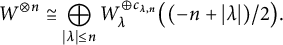(2.2) $$ \begin{align} W^{\otimes n} \cong \bigoplus_{\lvert\lambda\rvert \leq n} W_{\lambda}^{\oplus c_{\lambda,n}}\bigl((-n+\lvert\lambda\rvert)/2\bigr). \end{align} $$

Note that if $n \not \equiv \lvert \lambda \rvert \bmod 2$ , then $c_{\lambda ,n}=0$ . Note also that (2.2) holds with the same $c_{\lambda ,n}$ when replacing $\operatorname {\mathrm {GSp}}_{2g}$ with $\operatorname {\mathrm {USp}}_{2g}$ , i.e., replacing W by V and ignoring the multiplier representation. Note also that $W_{\lambda }^{\vee } \cong W_{\lambda }(\lvert \lambda \rvert )$ .

Let $\mathcal {X}=\mathcal {H}_g$ , $\mathcal {M}_g$ or $\mathcal {M}^{\text {nhyp}}_g$ for any $g \geq 2$ , or $\mathcal {X}=\mathcal {M}_{1,1}$ . Let $\pi : \mathcal {Y} \to \mathcal {X} $ be the universal object and define the $\ell $ -adic local system $\mathbb {V}=R^1 \pi _{*} \mathbb {Q}_{\ell }$ . To any irreducible representation of $\operatorname {\mathrm {GSp}}_{2g}$ (the symplectic pairing coming as above from the first cohomology group of the curves) corresponding to $\lambda $ , we can then use Schur functors to define a local system $\mathbb {V}_{\lambda }$ . Let $H^j_c$ denote compactly supported $\ell $ -adic cohomology and $\operatorname {\mathrm {Fr}}_q$ the geometric Frobenius acting on $\mathcal {X} \otimes \overline {\mathbb {F}}_q$ . For general results on étale cohomology of stacks, see, for instance, [Sun12].

For almost all primes p, we have $H^j_c(\mathcal {X} \otimes \mathbb {C}, \mathbb {V}_{\lambda }) \cong H^j_c(\mathcal {X} \otimes \overline {\mathbb {Q}}_p, \mathbb {V}_{\lambda }) \cong H^j_c(\mathcal {X} \otimes \overline {\mathbb {F}}_p, \mathbb {V}_{\lambda })$ . From this, we get bounds on $\dim _{\mathbb {Q}_{\ell }} H^j_c(\mathcal {X} \otimes \overline {\mathbb {F}}_p, \mathbb {V}_{\lambda })$ that are independent of p. This will tacitly be used below when we let q go to infinity.

Put $\overline {\mathcal {X}}=\mathcal {X} \otimes \overline {\mathbb {F}}_q$ . The Lefschetz trace formula and (2.2) then tell us that

$$ \begin{align*} S_n(q,\mathcal{X}) &=\sum_{j=0}^{2\dim \mathcal{X}} (-1)^j\operatorname{\mathrm{Tr}}(\operatorname{\mathrm{Fr}}_q,H^j_c(\overline{\mathcal{X}}, \mathbb{V}_1^{\otimes n}))\\ &=\sum_{\lambda} c_{\lambda,n} \, \sum_{j=0}^{2 \dim \mathcal{X}} (-1)^j \operatorname{\mathrm{Tr}}(\operatorname{\mathrm{Fr}}_q,H^j_c(\overline{\mathcal{X}}, \mathbb{V}_{\lambda})) \, q^{(n-\lvert\lambda\rvert)/2}\, \end{align*} $$

(compare [BFvdG14, Section 8]). Since $\mathbb {V}_{\lambda }$ is pure of weight $\lambda $ , it follows from Deligne’s theory of weights [Del80, Sun12] that the trace of Frobenius on $H^j_c(\overline {\mathcal {X}},\mathbb {V}_{\lambda })$ is equal (after choosing an embedding of $\overline {\mathbb {Q}}_{\ell }$ in $\mathbb {C}$ ) to a sum of complex numbers with absolute value at most $q^{(j+\lvert \lambda \rvert )/2}$ .

From this, we see that only when $j=2\dim \mathcal {X}$ can we get a contribution to $\mathfrak {a}_n(\mathcal {X})$ . Since $\mathcal {X}$ is a smooth Deligne–Mumford stack, Poincaré duality shows that for every i with $ 0 \leq i \leq 2\dim \mathcal {X}$ , we have

$$\begin{align*}H_c^{2\dim \mathcal{X}-i}(\overline{\mathcal{X}},\mathbb{V}_{\lambda}) \cong H^i(\overline{\mathcal{X}},\mathbb{V}_{\lambda})^{\vee}(-\dim \mathcal{X}-\lvert\lambda\rvert). \end{align*}$$

The zeroth cohomology group of a local system consists of the global invariants, and among the irreducible local systems, only the constant local system $\mathbb {V}_{(0)} \cong \mathbb {Q}_{\ell }$ has such. Moreover, $H^0(\overline {\mathcal {X}},\mathbb {Q}_{\ell })$ is one-dimensional, since $\mathcal {X}$ is irreducible. Finally, since the action of $\operatorname {\mathrm {Fr}}_q$ on $H^0(\overline {\mathcal {X}},\mathbb {Q}_{\ell })$ is trivial, we get by Poincaré duality that $\operatorname {\mathrm {Fr}}_q$ acts on $H_c^{2\dim \mathcal {X}}(\overline {\mathcal {X}},\mathbb {Q}_{\ell })$ by multiplication by $q^{\dim \mathcal {X}}$ . It follows that $\mathfrak {a}_n(\mathcal {X})=c_{(0),n}$ . This proves (1).

Assume now that $g \geq 3$ . From the work of Johnson and Hain, we know that $H^{1}(\mathcal {M}_g,\mathbb {V}_{\lambda })$ is nonzero if and only if $\lambda =(1,1,1)$ (see [Hai95, Joh83] and [Kab98, Theorem 4.1 and Corollary 4.2]). In these references, it is the rational Betti cohomology group of $\mathcal {M}_g$ over the complex numbers that is considered. Furthermore, $H^{1}(\mathcal {M}_g \otimes \overline {\mathbb {F}}_q,\mathbb {V}_{(1,1,1)})$ is one-dimensional and generated by the Gross–Schoen cycle, which lives in the second Chow group (see [PTY21, Remark 12.1 and Example 6.4]). Since this result also holds in $\ell $ -adic cohomology, as noted in [PTY21, Section 1.2], the action of $\operatorname {\mathrm {Fr}}_q$ on this cohomology group is by multiplication by $q^2$ .

Recall that $\dim \mathcal {M}_g=3g-3$ . By Poincaré duality, we find that the action of $\operatorname {\mathrm {Fr}}_q$ on $H_c^{6g-7}(\mathcal {M}_g \otimes \overline {\mathbb {F}}_q,\mathbb {V}_{(1,1,1)})$ is by $q^{3g-3+3-2}$ . We can now conclude the following. If n is even, then $c_{(1,1,1),n}=0$ , and so every eigenvalue of Frobenius contributing to $q^{3g-3+n/2}c_{(0),n}-S_n(q,\mathcal {M}_g)$ has absolute value at most $q^{3g-4+n/2}$ . If n is odd, then $c_{(0),n}=0$ , and so there are no eigenvalues of Frobenius contributing to $S_n(q,\mathcal {M}_g)$ of absolute value $q^{3g-3+n/2}$ and we can conclude by the above that $\mathfrak {b}_n(\mathcal {M}_g)=c_{(1,1,1),n}$ . This proves (2.1).

Because of the hyperelliptic involution, $H_c^{i}(\mathcal {M}_2,\mathbb {V}_{\lambda })=0$ for all $\lambda $ such that $\lvert \lambda \rvert $ is odd. Moreover, $H^{1}(\mathcal {M}_2,\mathbb {V}_{\lambda })$ is nonzero precisely when $\lambda =(2,2)$ . It is then one-dimensional and $\operatorname {\mathrm {Fr}}_q$ acts by multiplication by $q^3$ . This result is proven but not stated explicitly in [Pet15, Pet16], as explained in [Wat18, Corollary 6.7]. By Poincaré duality, $\operatorname {\mathrm {Fr}}_q$ acts on $H_c^{5}(\mathcal {M}_2,\mathbb {V}_{2,2})$ by multiplication by $q^{3+4-3}$ . Hence, for all even n, every eigenvalue of Frobenius contributing to $q^{3+n/2}c_{(0),n}-S_n(q,\mathcal {M}_2)$ has absolute value at most $q^{3+(n-2)/2}$ . This proves (2.1).

Statement (4) is only a reformulation of the properties of $\mathfrak {a}_n(\mathcal {M}_g)$ and $\mathfrak {b}_n(\mathcal {M}_g)$ proven above.

Finally, for every $k \geq 1$ , put . The polynomial $\mathbf {s}_{\langle (1,1,1)\rangle }(x_1,\ldots ,x_g)$ equals

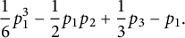$$\begin{align*}\frac{1}{6}p_1^3-\frac{1}{2}p_1p_2+\frac{1}{3}p_3-p_1. \end{align*}$$

The irreducible representations of $\operatorname {\mathrm {USp}}_{2g}$ are self-dual. As a consequence, if U is a representation of $\operatorname {\mathrm {USp}}_{2g}$ , then the number of times the representation $V_{\lambda }$ appears in U equals the number of times the trivial representation appears in $V_{\lambda } \otimes U$ . If $A \in \operatorname {\mathrm {USp}}_{2g}$ has eigenvalues $\alpha _1,\ldots ,\alpha _g,\alpha _1^{-1},\ldots ,\alpha _g^{-1}$ , with $\alpha _j=e^{i\theta _j}$ for $j=1,\ldots ,g$ , then $p_k(\alpha _1,\ldots ,\alpha _g)=w_k(\theta _1,\ldots ,\theta _g)$ . Statement (5) now follows from (2.1).

Remark 2.2 Why did we not define $\mathfrak {b}_n$ for $\mathcal {M}_{1,1}$ ? For every prime p and $n> 0$ , it follows from [Del71] (see also [Bir68] and [BFvdG14, Section 2]) that

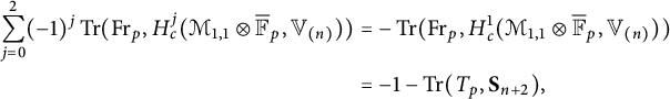$$ \begin{align*} \sum_{j=0}^{2} (-1)^j\operatorname{\mathrm{Tr}}(\operatorname{\mathrm{Fr}}_p,H^j_c(\mathcal{M}_{1,1} \otimes \overline{\mathbb{F}}_p, \mathbb{V}_{(n)})) &=-\operatorname{\mathrm{Tr}}(\operatorname{\mathrm{Fr}}_p,H^1_c(\mathcal{M}_{1,1} \otimes \overline{\mathbb{F}}_p, \mathbb{V}_{(n)}))\\ &=-1-\operatorname{\mathrm{Tr}}(T_p,\mathbf{S}_{n+2}), \end{align*} $$

where $T_p$ is the pth Hecke operator acting on $\mathbf {S}_{n+2}$ , the (complex) vector space of elliptic modular cusp forms of level $1$ and weight $n+2$ . Moreover, for every prime power q, the eigenvalues of $\operatorname {\mathrm {Fr}}_q$ acting on $H^1_c(\mathcal {M}_{1,1} \otimes \overline {\mathbb {F}}_p, \mathbb {V}_{(n)})$ will have absolute value $q^{(n+1)/2}$ . It is in general not clear that the limit

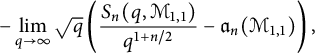(2.3) $$ \begin{align} -\lim_{q \to \infty} \sqrt{q} \left( \frac{S_n(q, \mathcal{M}_{1,1})}{q^{1+n/2}}-\mathfrak{a}_n(\mathcal{M}_{1,1})\right), \end{align} $$

which would be the way to define $\mathfrak {b}_n(\mathcal {M}_{1,1})$ , always exists when n is even. (For odd n, $S_n(q,\mathcal {M}_{1,1})=0$ ; hence, the limit (2.3) will be $0$ .)

For even $0 \leq n \leq 8$ , the limit (2.3) is also $0$ since there are no elliptic cusp forms level $1$ and weight less than or equal to $10$ . We then have that $S_{10}(p,\mathcal {M}_{1,1})=42p^6-\operatorname {\mathrm {Tr}}(T_p, \mathbf {S}_{12})+O(p^5)$ and $S_{12}(p,\mathcal {M}_{1,1})=132p^7-11p \cdot \operatorname {\mathrm {Tr}}(T_p, \mathbf {S}_{12})+O(p^6)$ . The so-called Frobenius angle, $0 \leq \varphi _p \leq \pi $ , of the Hecke eigenform (the Ramanujan $\Delta $ function) in the one-dimensional space $\mathbf {S}_{12}$ is defined by . The Sato–Tate conjecture for $\Delta $ (proven in [BLGHT11]) then tells us that there are sequences of primes $p^{\prime }_1,p^{\prime }_2,\ldots $ and $p^{\prime \prime }_1,p^{\prime \prime }_2,\ldots $ such that the Frobenius angles of $a_{p^{\prime }_1},a_{p^{\prime }_2},\ldots $ (respectively, $a_{p^{\prime \prime }_1},a_{p^{\prime \prime }_2},\ldots $ ) are all between $0$ and $\pi /3$ (respectively, $2\pi /3$ and $\pi $ ). This implies that the limit (2.3) does not exist for $n=10$ and $n=12$ . It is unlikely to exist for even $n>12$ , but the limit will then involve an interplay between different Hecke eigenforms.

In [BHLGR23, Theorem 3.9], it is shown that for fixed g, we have

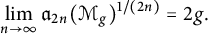$$\begin{align*}\lim_{n\rightarrow\infty}\mathfrak{a}_{2n}(\mathcal{M}_g)^{1/(2n)}=2g.\end{align*}$$

In the remainder of this section, we prove a similar result for $\mathfrak {b}_{2n+1}(\mathcal {M}_g)$ .

Proposition 2.3 For fixed $g \geq 3$ , one has

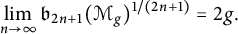$$\begin{align*}\lim_{n\rightarrow\infty} \mathfrak{b}_{2n+1}(\mathcal{M}_g)^{1/(2n+1)}=2g. \end{align*}$$

Proof Consider the functions $w_1$ and on . The maximum value of $\lvert w_1\rvert $ is attained at exactly two points in X, namely the points and . We have $w_1(x) = 2g$ and $w_1(y) = -2g$ , and we also have $f(x) = (2/3)(2g^3-3g^2-2g)> 0$ and $f(y) = (-2/3)(2g^3-3g^2-2g) < 0$ .

Let V be the (open) subset of X where $w_1 f> 0$ , so that x and y both lie in V, and let $W = X\setminus V$ . Let M be the supremum of $\lvert w_1\rvert $ on W, so that $M < 2g$ . For $\varepsilon \in (0,2g-M)$ , let $U_\varepsilon $ be the subset of X where $\lvert w_1 \rvert> 2g - \varepsilon $ , so that $U_\varepsilon \subset V$ , and let $V_\varepsilon = V\setminus U_\varepsilon $ .

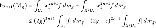
Then, for every n, we have

$$ \begin{align*} \mathfrak{b}_{2n+1}(\mathcal{M}_g) &= \int_X w_1^{2n+1} f \, d m_g \\ &= \int_{U_\varepsilon} w_1^{2n+1} f \, d m_g + \int_{V_\varepsilon} w_1^{2n+1} f \, d m_g + \int_{W} w_1^{2n+1} f \, d m_g \\ &\ge \int_{U_\varepsilon} w_1^{2n+1} f \, d m_g + \int_W w_1^{2n+1} f \, d m_g \\ &\ge (2g-\varepsilon)^{2n+1} \int_{U_\varepsilon} \lvert f\rvert \, d m_g - M^{2n+1} \int_W \lvert f\rvert\, d m_g, \end{align*} $$

where the third line follows from the fact that $w_1^{2n+1} f$ is positive on $V_\varepsilon $ and the fourth follows from the bounds on $\lvert w_1\rvert $ in $U_\varepsilon $ and W. Let and Then

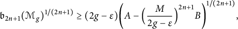$$\begin{align*}\mathfrak{b}_{2n+1}(\mathcal{M}_g)^{1/(2n+1)} \ge (2g-\varepsilon)\biggl(A - \Bigl(\frac{M}{2g-\varepsilon}\Bigr)^{2n+1} B\biggr)^{1/(2n+1)}, \end{align*}$$

and the rightmost factor tends to $1$ as $n\to \infty $ . Therefore, $\liminf \mathfrak {b}_{2n+1}(\mathcal {M}_g)^{1/(2n+1)} \ge 2g.$

We also have

$$ \begin{align*} \mathfrak{b}_{2n+1}(\mathcal{M}_g) &= \int_{U_\varepsilon} w_1^{2n+1} f \, d m_g + \int_{X\setminus U_\varepsilon} w_1^{2n+1} f \, d m_g\\ &\le (2g)^{2n+1}\int_{U_\varepsilon} \lvert f\rvert \, d m_g + (2g-\varepsilon)^{2n+1} \int_{X\setminus U_\varepsilon} \lvert f\rvert \, d m_g, \end{align*} $$

so if we let , then $\mathfrak {b}_{2n+1}(\mathcal {M}_g) \le (2g)^{2n+1} A + (2g-\varepsilon )^{2n+1} C,$ so

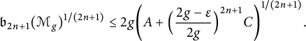$$\begin{align*}\mathfrak{b}_{2n+1}(\mathcal{M}_g)^{1/(2n+1)} \le 2g \biggl(A + \Bigl(\frac{2g-\varepsilon}{2g}\Bigr)^{2n+1} C\biggr)^{1/(2n+1)}. \end{align*}$$

Once again the rightmost factor tends to $1$ as $n\to \infty $ , so $\limsup \mathfrak {b}_{2n+1}(\mathcal {M}_g)^{1/(2n+1)} \le 2g,$ and the proposition is proven.

Remark 2.4 Let $\mathcal {X}_g$ be either $\mathcal {M}_g$ or $\mathcal {M}_{g,1}$ , where the latter denotes the moduli space of curves of genus g together with a marked point. For any $k \geq 0$ , $\lambda $ as in the proof of Theorem 2.1, and $g \geq \frac {3}{2}(k+1+|\lambda |)$ , there is an isomorphism in Betti cohomology, $H^k(\mathcal {X}_g,\mathbb {V}_{\lambda }) \cong H^k(\mathcal {X}_{g+1},\mathbb {V}_{\lambda })$ (see [Loo96, Theorem 1.1] and [Wah13]). These are called stable cohomology groups.

In [BDPW23, Theorem 3.5.12], there is an alternative formula to that of [Loo96, Theorem 1.1] for the dimensions of the stable cohomology groups of $\mathcal {M}_g$ . Using this formula, one can prove, in a way analogous to [BDPW23, Theorem 7.0.2], that if ${k < |\lambda |/3}$ and $g \geq \frac {3}{2}(k+1+|\lambda |)$ , then $H^k(\mathcal {M}_{g},\mathbb {V}_{\lambda })=0$ . It follows that for each k, there are finitely many $\lambda $ for which $H^k(\mathcal {M}_g,\mathbb {V}_{\lambda })$ , with $g = \lceil \frac {3}{2}(k+1+|\lambda |) \rceil $ , is nonzero. Again using [BDPW23, Theorem 3.5.12], we find, for instance, that there are 5 such $\lambda $ for $k=2$ (see below) and 14 such $\lambda $ for $k=3$ . Note also that for $g \geq \frac {3}{2}(k+1+|\lambda |)$ , $H^k(\mathcal {M}_{g},\mathbb {V}_{\lambda })$ is zero if $k+|\lambda |$ is odd.

The result above also holds in $\ell $ -adic cohomology. Moreover, every eigenvalue of Frobenius $F_q$ acting on the compactly supported $\ell $ -adic cohomology group $H_c^{6g-6-k}(\mathcal {M}_g,\mathbb {V}_{\lambda })$ , for $g \geq \frac {3}{2}(k+1+|\lambda |)$ , is equal to $q^{3g-3+(|\lambda |-k)/2}$ (see, for instance, [PTY21]).

In [MPPR24], it is shown that for $g \geq 3k+3$ (i.e., a bound that is independent of $\lambda $ ), there is an isomorphism in Betti cohomology, $H^k(\mathcal {M}_{g,1},\mathbb {V}_{\lambda }) \cong H^k(\mathcal {M}_{g+1,1},\mathbb {V}_{\lambda })$ . It should be possible to show that this leads to an isomorphism $H^k(\mathcal {M}_{g},\mathbb {V}_{\lambda }) \cong H^k(\mathcal {M}_{g+1},\mathbb {V}_{\lambda })$ for all $g \geq g_{\mathrm {stab}}(k)$ , with $g_{\mathrm {stab}}(k)$ a function that only depends upon k (cf. [CM09] and [BDPW23, Remark 3.5.11]). If we assume this to be true, then we can combine the results above with the techniques in the proof of Theorem 2.1 to conclude the following.

Let $d_{n,\lambda }$ denote the number of times the representation $V_{\lambda }$ appears in the $\operatorname {\mathrm {USp}}_{2g}$ -representation $V^{\otimes n}$ . Fix any $K\geq 0$ . Then, for any $n \geq 1$ and $g \geq g_{\mathrm {stab}}(K)$ , we have

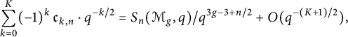(2.4) $$ \begin{align} \sum_{k=0}^K (-1)^k \, \mathfrak{c}_{k,n} \cdot q^{-k/2}=S_n(\mathcal{M}_g,q)/q^{3g-3+n/2}+O(q^{-(K+1)/2}), \end{align} $$

where

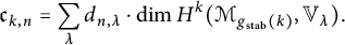$$\begin{align*}\mathfrak{c}_{k,n}=\sum_{\lambda}d_{n,\lambda} \cdot \dim H^k(\mathcal{M}_{g_{\mathrm{stab}}(k)},\mathbb{V}_{\lambda}). \end{align*}$$

From [BDPW23, Theorem 3.5.12], we can, for instance, compute that

$$\begin{align*}\mathfrak{c}_{2,n}=d_{n,(0)}+d_{n,(1^2)}+d_{n,(1^4)}+d_{n,(1^6)}+d_{n,(2^2,1^2)}. \end{align*}$$

Note that by Theorem 2.1, $\mathfrak {c}_{0,n}=\mathfrak {a}_n(\mathcal {M}_g)$ for $g \geq 2$ , $\mathfrak {c}_{1,n}=\mathfrak {b}_n(\mathcal {M}_g)$ for $g \geq 3$ , and equation (2.4) holds with $g_{\mathrm {stab}}(0)=2$ and $g_{\mathrm {stab}}(1)=3$ .

3 Convergence of moments of the measures $\mu _{q,g}$

Let $\mathcal {M}_g'(\mathbb {F}_q)$ be the set of $\mathbb {F}_q$ -isomorphism classes of curves of genus $g>1$ over $\mathbb {F}_q$ . If $g=1$ , we abuse notation and let $\mathcal {M}_1=\mathcal {M}_{1,1}$ be the moduli space of elliptic curves and $\mathcal {M}^{\prime }_1(\mathbb {F}_q)$ the set of $\mathbb {F}_q$ -isomorphism classes of elliptic curves over $\mathbb {F}_q$ . Define a measure $\mu _{q,g}$ by

where is the normalized trace of C and $\delta _{\tau (C)}$ is the Dirac $\delta $ measure supported at $\tau (C)$ . We see that $\mu _{q,g}$ is a discrete probability measure on , since

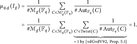$$ \begin{align*} \mu_{q,g}(I_g) &= \frac{1}{\# \mathcal{M}_g(\mathbb{F}_q)} \sum_{C\in \mathcal{M}_g'(\mathbb{F}_q)} \frac{1}{\#\operatorname{\mathrm{Aut}}_{\mathbb{F}_q}(C)} \\ &= \frac{1}{\# \mathcal{M}_g(\mathbb{F}_q)} \sum_{C\in \mathcal{M}_g(\mathbb{F}_q)} \underbrace{\sum_{C' \in \operatorname{\mathrm{Twist}}(C)} \frac{1}{\#\operatorname{\mathrm{Aut}}_{\mathbb{F}_q}(C)}}_{=\,1 \; \text{by [vdGvdV92, Prop. 5.1]}} = 1. \end{align*} $$

We can introduce $\mathcal {N}_{q,g}(\tau )$ defined by

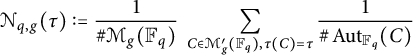
and rewrite $\mu _{q,g} = \sum _{\tau \in I_g} \mathcal {N}_{q,g}(\tau ) \delta _\tau $ . Note that the definition of $\mathcal {N}_{q,g}(\tau )$ differs from the ones of [LRRS14, Appendix B] and [LRR⁺19, Section 4], in particular by a factor of $\sqrt {q}$ (this factor will appear again in Section 4, but this definition is more natural for the measure).

From [Lac16, Remark 3.5], as a direct consequence of Katz–Sarnak results [KS99, Theorems 10.7.12 and 10.8.2], there exists a probability measure $\mu _g \colon I_g \to \mathbb {R}$ with a $\mathcal {C}^{\infty }$ density function ${\mathfrak {f}}_g$ such that we have weak convergence of $\mu _{q,g}$ to $\mu _g$ . Writing

$$\begin{align*}{\mathfrak{f}}_g(\tau)=\int_{A_{\tau}} dm_g \; \textrm{with} \; A_{\tau}=\bigl\{(\theta_1,...,\theta_g)\in[0,\pi]^g:\,\textstyle\sum_{j}2\cos\theta_j = \tau\bigr\},\end{align*}$$

we see this is equivalent to

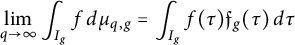(3.1) $$ \begin{align}\lim_{q \to \infty} \int_{I_g} f \, d\mu_{q,g} = \int_{I_g} f(\tau){\mathfrak{f}}_g(\tau)\,d\tau \end{align} $$

for all continuous functions $f\colon I_g \to \mathbb {R}$ . Moreover, for all polynomial functions ³ $P\colon I_g \to \mathbb {R}$ ,

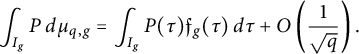(3.2) $$ \begin{align} \int_{I_g} P \, d\mu_{q,g} = \int_{I_g} P(\tau){\mathfrak{f}}_g(\tau)\,d\tau + O\left(\frac{1}{\sqrt{q}}\right). \end{align} $$

We will now find a refinement of (3.2) when $g \geq 2$ .

Theorem 3.1 Let

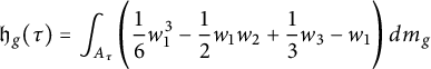(3.3) $$ \begin{align} {\mathfrak{h}}_g(\tau)=\int_{A_{\tau}} \Bigg(\frac{1}{6}w_1^3-\frac{1}{2}w_1w_2+\frac{1}{3}w_3-w_1 \Bigg)\, d m_g \end{align} $$

be the function whose nth moments are equal to the numbers $\mathfrak {b}_n(\mathcal {M}_g)$ given by the expression (2.1). For $g\geq 2$ and every polynomial function $P : I_g \to \mathbb {R}$ , we have

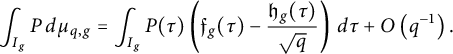(3.4) $$ \begin{align} \int_{I_g} P \, d\mu_{q,g} = \int_{I_g} P(\tau) \left({\mathfrak{f}}_g(\tau)-\frac{{\mathfrak{h}}_g(\tau)}{\sqrt{q}}\right)\,d\tau + O\left(q^{-1}\right). \end{align} $$

Proof Notice that

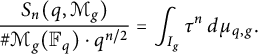$$\begin{align*}\frac{S_n(q,\mathcal{M}_g)}{\# \mathcal{M}_g(\mathbb{F}_q) \cdot q^{n/2}} = \int_{I_g} \tau^n \,d\mu_{q,g}. \end{align*}$$

Using Deligne’s theory of weights, as in the proof of Theorem 2.1, we find that

$$\begin{align*}\#\mathcal{M}_g(\mathbb{F}_q)= \operatorname{\mathrm{Tr}} \bigl(\mathrm{Fr}_q,H_c^{6g-6}(\mathcal{M}_g,\mathbb{Q}_{\ell})\bigr)+O\left(q^{3g-4}\right)=q^{3g-3}+O\left(q^{3g-4}\right), \end{align*}$$

since $\mathcal {M}_g$ is irreducible of dimension $3g-3$ . Hence,

$$\begin{align*}\frac{S_n(q,\mathcal{M}_g)}{\# \mathcal{M}_g(\mathbb{F}_q) \cdot q^{n/2}}= \frac{S_n(q,\mathcal{M}_g)}{q^{3g-3+n/2}}+ O(q^{-1}).\end{align*}$$

Using Theorem 2.1 (4) for $g \geq 2$ , we then get

$$ \begin{align*} \int_{I_g} \tau^n \,d\mu_{q,g} &= \frac{S_n(q,\mathcal{M}_g)}{\# \mathcal{M}_g(\mathbb{F}_q) \cdot q^{n/2}} \\ &= \frac{S_n(q,\mathcal{M}_g)}{q^{3g-3+n/2}}+ O(q^{-1})\\ &= \mathfrak{a}_n(\mathcal{M}_g) - \frac{\mathfrak{b}_n(\mathcal{M}_g)}{\sqrt{q}} + O(q^{-1}) \\ &= \int_{I_g} \tau^n \left({\mathfrak{f}}_g(\tau)-\frac{{\mathfrak{h}}_g(\tau)}{\sqrt{q}}\right)\,d\tau + O\left(q^{-1}\right).\\[-42pt] \end{align*} $$

4 The elliptic and hyperelliptic cases: results and experiments

Katz–Sarnak results show that for every interval $J\subseteq I_g$ , the probability that a random curve of genus g over $\mathbb {F}_q$ (or a random hyperelliptic curve of genus g over $\mathbb {F}_q$ ) has normalized trace in J tends toward a fixed value as $q\to \infty $ , this value being $\int _J {\mathfrak {f}}_g(\tau ) \,d\tau $ , where ${\mathfrak {f}}_g$ is the density function for the measure $\mu _g$ defined at the beginning of Section 3. Here, the interval J is fixed, and we let q tend to infinity. One can wonder how rapid this convergence is. For instance, suppose the interval J has length x. How large must q become in order for the actual probability that a normalized trace lies in J is well-approximated by the Katz–Sarnak prediction? Could it even be the case that the approximation is reasonably good when q is as large as $1/x^2$ , so that $x\approx 1/\sqrt {q}$ and there is exactly one integer t with $t/\sqrt {q}\in J$ ? In other words, can we use the Katz–Sarnak distribution to estimate the number of curves over $\mathbb {F}_q$ with a given trace? Since the measures $\mu _{q,g}$ converge weakly to $\mu _g$ , one might hope that for every $\tau \in I_g$ , the integral of $\mu _{q,g}$ over an interval of length $1/\sqrt {q}$ containing $\tau $ would be close to the integral of $\mu _g$ over this interval. If we let t be the unique integer such that $t/\sqrt {q}$ is contained in this interval, this optimistic approximation then translates to

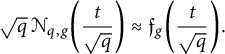$$\begin{align*}\sqrt{q}\,\mathcal{N}_{q,g}\biggl(\frac{t}{\sqrt{q}}\biggr) \approx {\mathfrak{f}}_g\biggl(\frac{t}{\sqrt{q}}\biggr). \end{align*}$$

Since $\mathcal {N}_{q,g}(t/\sqrt {q})$ gives us the weighted number of curves with trace t, if this approximation is close to the truth, we would have a good estimate for the number of such curves.

Remark 4.1 We do not know how to prove that this estimate holds, and indeed we will see below that it does not hold, without modification, for hyperelliptic curves. One consequence of this estimate, however, is the much weaker statement that for every fixed value of t, the value of $\mathcal {N}_{q,g}(t)$ converges to $0$ as q increases. It is at least easy to show that this weaker statement holds for $t=0$ , by the following argument.

Given $\varepsilon>0$ , let $f\colon I_g\to [0,1]$ be a continuous function with $f(0) = 1$ and with $f(\tau )=0$ when $\lvert \tau \rvert \ge \varepsilon $ . From (3.1), we find that for q large enough, we have

$$\begin{align*}\biggl\lvert\,\int_{I_g} f \, d\mu_{q,g} - \int_{I_g} f(\tau) {\mathfrak{f}}_g(\tau) \, d\mu_{g}\biggr\rvert \leq \varepsilon.\end{align*}$$

Hence,

$$\begin{align*}0 \leq \mathcal{N}_{q,g}(0) \leq \int_{I_g} f \, d\mu_{q,g} \leq \int_{\lvert\tau\rvert<\varepsilon} f(\tau) {\mathfrak{f}}_g(\tau)\,d\tau +\varepsilon \leq (2\left\|{\mathfrak{f}}_g\right\|_\infty+1) \varepsilon. \end{align*}$$

As we intimated in the preceding remark, for hyperelliptic curves, we can prove that the naïve approximation for $\mathcal {N}_{q,g}$ described above cannot hold. To state our result precisely, we introduce a function $\mathcal {N}^{\text {hyp}}_{q,g}(\tau )$ , which we define analogously to how we defined $\mathcal {N}_{q,g}(\tau )$ :

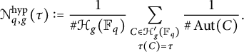
Here, by $\mathcal {H}_g(\mathbb {F}_q)$ , we mean the set of $\overline {\mathbb {F}}_q$ -isomorphism classes of hyperelliptic curves of genus g over $\mathbb {F}_q$ , and by $\mathcal {H}_g'(\mathbb {F}_q)$ , we mean the set of $\mathbb {F}_q$ -isomorphism classes of such curves. Note that for an integer t in $I_g$ , the value $q^{2g-1} \mathcal {N}^{\text {hyp}}_{q,g}(t/\sqrt {q})$ is then the weighted number of genus-g hyperelliptic curves over $\mathbb {F}_q$ with trace t.

Proposition 4.2 Fix $g>1$ and $\varepsilon \in [0,2g)$ , let , and let $v = \int _{2g-\varepsilon }^{2g} {\mathfrak {f}}_g(\tau ) \,d\tau $ . Suppose there are constants $b_g\le c_g$ such that for every sufficiently large prime power q and for every integer t in $[-(2g-\varepsilon )\sqrt {q}, (2g-\varepsilon )\sqrt {q}\,]$ , we have

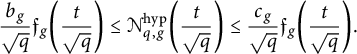$$\begin{align*}\frac{b_g}{\sqrt{q}} {\mathfrak{f}}_g\biggl(\frac{t}{\sqrt{q}}\biggr) \le \mathcal{N}^{\text{hyp}}_{q,g}\biggl(\frac{t}{\sqrt{q}}\biggr) \le \frac{c_g}{\sqrt{q}} {\mathfrak{f}}_g\biggl(\frac{t}{\sqrt{q}}\biggr). \end{align*}$$

Then $b_g\le (1-r_g)/(1-2v)$ and $c_g\ge (1 + r_g - 4v)/(1-2v)$ .

The proof is based on the following lemma.

Lemma 4.3 Fix $g>1$ , and let $r_g$ be as in Proposition 4.2. If q is an odd prime power, then

$$\begin{align*}\sum_{t\,\text{even}} \mathcal{N}^{\text{hyp}}_{q,g}\biggl(\frac{t}{\sqrt{q}}\biggr) = \frac{1+r_g}{2} + O\Bigg(\frac1q\Bigg) \quad \text{and}\quad \sum_{t\,\text{odd}} \mathcal{N}^{\text{hyp}}_{q,g}\biggl(\frac{t}{\sqrt{q}}\biggr) = \frac{1-r_g}{2} + O\Bigg(\frac1q\Bigg). \end{align*}$$

Proof Fix an odd prime power q, fix a nonsquare $n\in \mathbb {F}_q$ , and consider the set H consisting of all pairs $(c,f)$ , where $c\in \{1,n\}$ and $f\in \mathbb {F}_q[x]$ is a monic separable polynomial of degree $2g+1$ or $2g+2$ . A result of Carlitz [Car32, Section 6] shows that $\#H = 2q^{2g+2} - 2q^{2g}.$ The group $\operatorname {\mathrm {PGL}}_2(\mathbb {F}_q)$ acts on H: Given a matrix $[\begin {smallmatrix}r&s\\t&u\end {smallmatrix}]$ and an element $(c,f)$ of H, let $(d,g)$ be the unique element of H such that

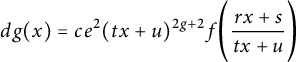$$\begin{align*}d g(x) = c e^2 (tx+u)^{2g+2} f\Bigg(\frac{rx+s}{tx+u}\Bigg) \end{align*}$$

for some $e\in \mathbb {F}_q^\times .$ Note that the stabilizer of $(c,f)$ is isomorphic to the reduced automorphism group $\operatorname {\mathrm {RedAut}}(C)$ of the hyperelliptic curve $C\colon y^2 = cf$ , that is, the quotient of the full automorphism group of C by the subgroup generated by the hyperelliptic involution.

The map $\gamma $ that sends $(c,f)\in H$ to the hyperelliptic curve $y^2 = c f$ takes H onto $\mathcal {H}^{\prime }_g(\mathbb {F}_q)$ . Given a curve $C\in \mathcal {H}^{\prime }_g(\mathbb {F}_q)$ , let $(c,f)\in H$ be such that $\gamma ((c,f)) = C$ . Then

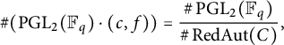$$\begin{align*}\#(\operatorname{\mathrm{PGL}}_2(\mathbb{F}_q)\cdot (c,f)) = \frac{\#\operatorname{\mathrm{PGL}}_2(\mathbb{F}_q)}{\#\operatorname{\mathrm{RedAut}}(C)}, \end{align*}$$

so that

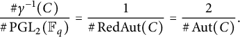(4.1) $$ \begin{align} \frac{ \#\gamma^{-1}(C)}{\#\operatorname{\mathrm{PGL}}_2(\mathbb{F}_q)} = \frac{1}{\#\operatorname{\mathrm{RedAut}}(C)} = \frac{2}{\#\operatorname{\mathrm{Aut}}(C)}. \end{align} $$

Let $H_{\text {even}}$ be the subset of H consisting of the pairs $(c,f)$ such that the curve $\gamma (c,f)$ has even trace. Let $H^{\prime }_{\text {even}}$ be the subset of H consisting of the pairs $(c,f)$ such that f has degree $2g+2$ and has an even number of roots. Then $H^{\prime }_{\text {even}}\subseteq H_{\text {even}}$ , and $H_{\text {even}}\setminus H^{\prime }_{\text {even}}$ consists of pairs $(c,f)\in H_{\text {even}}$ such that f has degree $2g+1$ . Therefore,

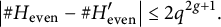$$\begin{align*}\bigl\vert \#H_{\text{even}} - \#H^{\prime}_{\text{even}}\bigr\vert \le 2q^{2g+1}. \end{align*}$$

Leont’ev [Leo06a, Lemma 4, p. 302] gives the generating function for the number of (not necessarily separable) monic polynomials of a fixed degree over $\mathbb {F}_q$ that have a given number of roots. To find the number of such polynomials with an even number of roots, we simply need to take the average of the values of this generating function evaluated at $-1$ and at $1$ . We find that

$$\begin{align*}\#\left\{\begin{array}{@{}ll@{}}\textrm{monic}\ \textrm{polynomials}\ \textrm{of}\ \textrm{degree}\ 2g+2\\ \textrm{over}\ {\mathbb{F}_q}\ \textrm{with}\ \textrm{an}\ \textrm{even}\ \textrm{number}\ \textrm{of}\ \textrm{roots}\end{array} \right\} = \frac{1+r_g}{2} q^{2g+2} + O(q^{2g+1}). \end{align*}$$

The result of Carlitz mentioned earlier shows that

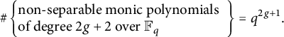$$\begin{align*}\#\left\{\begin{array}{@{}ll@{}} \textrm{non-separable}\ \textrm{monic}\ \textrm{polynomials}\\ \textrm{of}\ \textrm{degree}\ {2g+2}\ \textrm{over}\ {\mathbb{F}_q}\end{array}\right\} =q^{2g+1}. \end{align*}$$

Therefore, $\# H^{\prime }_{\text {even}} = (1+r_g) q^{2g+2} + O(q^{2g+1})$ , so that $\# H_{\text {even}} = (1+r_g) q^{2g+2} + O(q^{2g+1})$ as well.

Using (4.1), we see that

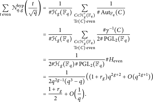$$ \begin{align*} \sum_{t \,\text{even}} \mathcal{N}^{\text{hyp}}_{q,g}\biggl(\frac{t}{\sqrt{q}}\biggr) &= \frac{1}{\#\mathcal{H}_g(\mathbb{F}_q)} \sum_{\substack{C\in \mathcal{H}^{\prime}_g(\mathbb{F}_q)\\ \operatorname{\mathrm{Tr}}(C)\, \text{even}}} \frac{1}{\#\operatorname{\mathrm{Aut}}_{\mathbb{F}_q}(C)}\\ &= \frac{1}{\#\mathcal{H}_g(\mathbb{F}_q)} \sum_{\substack{C\in \mathcal{H}^{\prime}_g(\mathbb{F}_q)\\ \operatorname{\mathrm{Tr}}(C)\, \text{even}}} \frac{\#\gamma^{-1}(C)}{2\#\operatorname{\mathrm{PGL}}_2(\mathbb{F}_q)}\\ &= \frac{1}{2\#\mathcal{H}_g(\mathbb{F}_q)\#\operatorname{\mathrm{PGL}}_2(\mathbb{F}_q)} \#H_{\text{even}}\\ &=\frac{1}{2 q^{2g-1} (q^3-q)}\bigl((1+r_g)q^{2g+2} + O(q^{2g+1})\bigr)\\ &=\frac{1+r_g}{2} + O\Bigl(\frac{1}{q}\Bigr). \end{align*} $$

This gives us the first equality in the conclusion of the lemma. The second follows analogously.

Proof of Proposition 4.2

Suppose the hypothesis of the proposition holds for a given g and $\varepsilon $ . For a given q, we let $m = \lfloor 2\sqrt {q} \rfloor $ and we consider several subintervals of $[-2g\sqrt {q},2g\sqrt {q}]$ :

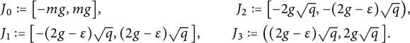
Now we interpret the sum

in two ways. On the one hand, from Lemma 4.3, we have

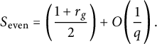$$\begin{align*}S_{\text{even}} = \biggl(\frac{1+r_g}{2}\biggr) + O\Bigg(\frac{1}{q}\Bigg)\,. \end{align*}$$

On the other hand, for q large enough, we have

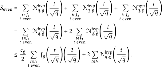(4.2) $$ \begin{align} S_{\text{even}} \notag &= \sum_{\substack{t\in J_1\\ t \ \text{even}}} \mathcal{N}^{\text{hyp}}_{q,g}\biggl(\frac{t}{\sqrt{q}}\biggr) + \sum_{\substack{t\in J_2\\ t \ \text{even}}} \mathcal{N}^{\text{hyp}}_{q,g}\biggl(\frac{t}{\sqrt{q}}\biggr) + \sum_{\substack{t\in J_3\\ t \ \text{even}}} \mathcal{N}^{\text{hyp}}_{q,g}\biggl(\frac{t}{\sqrt{q}}\biggr)\\ \notag &= \sum_{\substack{t\in J_1\\ t \ \text{even}}} \mathcal{N}^{\text{hyp}}_{q,g}\biggl(\frac{t}{\sqrt{q}}\biggr) + 2\sum_{\substack{t\in J_3\\ t \ \text{even}}} \mathcal{N}^{\text{hyp}}_{q,g}\biggl(\frac{t}{\sqrt{q}}\biggr)\\ & \le \frac{c_g}{2} \sum_{\substack{t\in J_1\\ t \ \text{even}}} {\mathfrak{f}}_g\biggl(\frac{t}{\sqrt{q}}\biggr) \biggl(\frac{2}{\sqrt{q}}\biggr) + 2\sum_{t\in J_3} \mathcal{N}^{\text{hyp}}_{q,g}\biggl(\frac{t}{\sqrt{q}}\biggr) \,. \end{align} $$

The first sum in (4.2) is a Riemann sum for the integral of ${\mathfrak {f}}_g(\tau ) \, d\tau $ over the interval $[-2g+\varepsilon , 2g-\varepsilon ]$ , so as $q\to \infty $ the first term in (4.2) approaches $c_g(1-2v)/2$ . The second sum is the measure, with respect to $\mu _{q,g}$ , of the interval $[2g-\varepsilon ,2g]$ . Since the $\mu _{q,g}$ converge weakly to $\mu _g$ , the second term of (4.2) approaches $2v$ as $q\to \infty $ .

Combining these two interpretations of $S_{\text {even}}$ , we find that

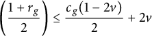$$\begin{align*}\biggl(\frac{1+r_g}{2}\biggr) \le \frac{c_g(1-2v)}{2} + 2v \end{align*}$$

so that $c_g \ge (1 + r_g - 4v)/(1-2v)$ .

Similarly, we can consider the sum

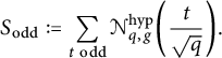
From Lemma 4.3, we see that

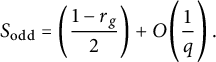$$\begin{align*}S_{\text{odd}} = \biggl(\frac{1-r_g}{2}\biggr) + O\Bigg(\frac{1}{q}\Bigg)\,. \end{align*}$$

But we also have

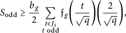$$\begin{align*}S_{\text{odd}} \ge \frac{b_g}{2} \sum_{\substack{t\in J_1\\ t \ \text{odd}}} {\mathfrak{f}}_g\biggl(\frac{t}{\sqrt{q}}\biggr) \biggl(\frac{2}{\sqrt{q}}\biggr), \end{align*}$$

and the expression on the right approaches $b_g(1-2v)/2$ as $q\to \infty $ . This shows that

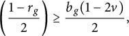$$\begin{align*}\biggl(\frac{1-r_g}{2}\biggr) \ge \frac{b_g(1-2v)}{2}, \end{align*}$$

so we find that $b_g\le (1-r_g)/(1-2v)$ .

Remark 4.4 In the statement of Proposition 4.2, we only assume that the condition on $\mathcal {N}^{\text {hyp}}_{q,g}(t/\sqrt {q})$ holds for t more than $\varepsilon \sqrt {q}$ away from the ends of the interval $[-2g\sqrt {q}, 2g\sqrt {q}\,]$ because when $\lvert t\rvert> g\lfloor 2\sqrt {q}\rfloor $ we have $\mathcal {N}^{\text {hyp}}_{q,g}(t/\sqrt {q}) = 0$ . If we did not exclude the tail ends of the interval, the hypothesis of the proposition would only hold if we took $b_g=0$ , which is not an interesting approximation.

Figure 1 shows the value of $\mathcal {N}^{\text {hyp}}_{q,g}(t/\sqrt {q})$ for all integers $t\in [-4\sqrt {q},4\sqrt {q}]$ , where $q = 1,009$ , together with the density function ${\mathfrak {f}}_2$ for the limiting Katz–Sarnak measure, scaled by the two factors $b=38/45$ and $c = 52/45$ given by Proposition 4.2 for $g=2$ and $\varepsilon =0$ .

The key to Proposition 4.2 is the imbalance between the likelihood of even versus odd traces for hyperelliptic curves. The obvious work-around would be to scale the counts for the even and odd traces by the factors given in the proposition for $\varepsilon =0$ . One can ask whether the scaled curve counts then better match the limiting Katz–Sarnak distribution. Figure 2 suggests that perhaps this parity factor is the main obstruction to obtaining decent estimates from the naïve Katz–Sarnak approximation.

The proof of Proposition 4.2 carries through for elliptic curves exactly as it does for hyperelliptic curves of a given genus $g>1$ . We do not include genus- $1$ curves in the statement of the proposition, however, because as we will see in Proposition 4.5, for $g=1$ there is no value of $c_1$ that satisfies the hypothesis of the proposition when $\varepsilon \le 1$ , while the conclusion of the proposition is trivial when $\varepsilon>1$ because the resulting upper bound on $b_1$ will be greater than $1$ and the lower bound on $c_1$ will be less than $1$ .

When $g=1$ , the density function of the limiting Katz–Sarnak measure on $I_1$ is ${{\mathfrak {f}}_1= (2\pi )^{-1}\sqrt {4-\tau ^2}}$ . Let $N_{q,t}$ denote the weighted number of elliptic curves over $\mathbb {F}_q$ with trace t. For some values of t in $[-2\sqrt {q},2\sqrt {q}\,]$ , we have $N_{q,t} = 0$ ; in addition to those t with $\lvert t\rvert> \lfloor 2\sqrt {q}\rfloor $ , this happens for most values of t that are not coprime to q. But even if we exclude these values, and even if we restrict attention to values of t that are near the center of the interval $[-2\sqrt {q},2\sqrt {q}\,]$ , the following proposition shows that we cannot hope to approximate $N_{q,t}$ by the quantity

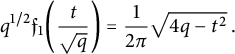$$\begin{align*}q^{1/2} {\mathfrak{f}}_1\biggl(\frac{t}{\sqrt{q}}\biggr) = \frac{1}{2\pi}\sqrt{4q - t^2}\,.\end{align*}$$

Proposition 4.5 For every $c>0$ , there are infinitely many values of q and t such that $\lvert t \rvert \le \sqrt {q}$ and $N_{q,t}> c \sqrt {4q-t^2}$ .

Proof Let $\Delta _0$ be a fundamental quadratic discriminant with $\Delta _0<-4$ , and let $\chi $ be the quadratic character modulo $\Delta _0$ . For a given value of n, let f be the product of the first n primes p that are inert in $\mathbb {Q}(\sqrt {\Delta _0})$ . Since the product over all inert primes of $1+1/p$ diverges (see [Cox13, Lemma 1.14] and [Apo76, Exercise 6, p. 176]), when n is large enough, we have

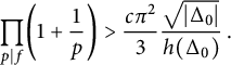$$\begin{align*}\prod_{p\mid f} \biggl(1 + \frac{1}{p}\biggr)> \frac{c\pi^2}{3} \frac{\sqrt{\lvert\Delta_0\rvert}}{h(\Delta_0)}\,. \end{align*}$$

Choose n so that this holds, and let $q_0$ be a prime of the form $x^2 - f^2\Delta _0 y^2$ , where x and y are positive integers. Note that x must be coprime to $q_0$ because $0<x<q_0$ . Let $\varpi = x + fy\sqrt {\Delta _0}$ , viewed as an element of the upper half plane. Since x is coprime to $q_0$ , $\varpi $ is the Weil number of an isogeny class of ordinary elliptic curves over $\mathbb {F}_{q_0}$ .

Let $\theta $ be the argument of $\varpi $ , and let m be the smallest integer such that $\pi /3\le m\theta < 2\pi /3$ . Write $\varpi ^m = u + fv\sqrt {\Delta }$ for integers u and v, let $q = q_0^m = u^2 - f^2v^2\Delta $ , and let $t = 2u$ . Then $\varpi ^m$ is the Weil number for an isogeny class $\mathcal {I}$ of ordinary elliptic curves over $\mathbb {F}_q$ , and the trace of this isogeny class is t. We have $\lvert t\rvert \le \sqrt {q}$ because the argument of $\varpi ^m$ lies between $\pi /3$ and $2\pi /3$ .

The number of elliptic curves in the isogeny class $\mathcal {I}$ is equal to the Kronecker class number $H(\Delta )$ of the discriminant . By [How22, p. 696], we have

$$\begin{align*}H(\Delta) = h(\Delta_0) \prod_{p^e\parallel F} \Bigl(1 + \Bigl(1 - {\textstyle\frac{\chi(p)}{p}}\Bigr) (p + \cdots + p^e)\Bigr)\,, \end{align*}$$

where $F = 2fv$ , so

$$\begin{align*}\frac{H(\Delta)}{\sqrt{4q-t^2}} = \frac{h(\Delta_0)}{\sqrt{\lvert\Delta_0\rvert}} \prod_{p^e\parallel F} \Bigl(p^{-e} + \Bigl(1 - {\textstyle\frac{\chi(p)}{p}}\Bigr) (1 + p^{-1} + \cdots + p^{1-e})\Bigr)\,. \end{align*}$$

Now,

$$\begin{align*}p^{-e} + \Bigl(1 - {\textstyle\frac{\chi(p)}{p}}\Bigr) (1 + p^{-1} + \cdots + p^{1-e}) \ge \begin{cases} 1 + 1/p, & \text{if}\ \chi(p) = -1,\\ 1 - 1/p^2, & \text{if}\ \chi(p) \neq -1, \end{cases} \end{align*}$$

so we have

$$ \begin{align*} \frac{H(\Delta)}{\sqrt{4q-t^2}} &\ge \frac{h(\Delta_0)}{\sqrt{\lvert\Delta_0\rvert}} \prod_{\substack{p \mid F\\ \chi(p)=-1}}\Bigl(1 + \frac{1}{p}\Bigr) \prod_{\substack{p \mid F\\ \chi(p)\ne -1}}\Bigl(1 - \frac{1}{p^2}\Bigr)\\ &\ge \frac{h(\Delta_0)}{\sqrt{\lvert\Delta_0\rvert}} \prod_{p \mid f}\Bigl(1 + \frac{1}{p}\Bigr) \prod_{p}\Bigl(1 - \frac{1}{p^2}\Bigr)\\ &\ge \frac{h(\Delta_0)}{\sqrt{\lvert\Delta_0\rvert}} \biggl(\frac{c\pi^2}{3} \frac{\sqrt{\lvert\Delta_0\rvert}}{h(\Delta_0)}\biggr) \biggl(\frac{6}{\pi^2}\biggr)\\ &\ge 2c. \end{align*} $$

Since the curves in $\mathcal {I}$ are ordinary and the discriminants of their endomorphism rings are neither $-3$ nor $-4$ , they all have automorphism groups of order $2$ , so $N_{q,t} = H(\Delta )/2$ . It follows that

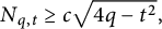$$\begin{align*}N_{q,t} \ge c \sqrt{4q-t^2}, \end{align*}$$

as claimed.

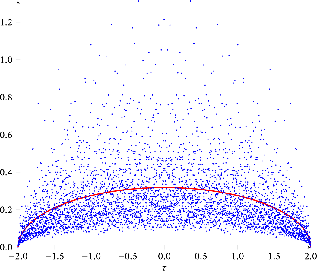
Figure 3: Data for elliptic curves over $\mathbb {F}_q$ for $q=1,000,003$ . The blue dots are the points $(t/\sqrt {q},N_{q,t}/\sqrt {q})$ for $t\in [-2000,2000]$ , where $N_{q,t}$ is the weighted number of elliptic curves over $\mathbb {F}_q$ with trace t. The red curve is the density function ${\mathfrak {f}}_1(\tau ) = (2\pi )^{-1}\sqrt {4-\tau ^2}$ of the distribution $\mu _1$ .

Figure 3 shows the weighted number of elliptic curves over $\mathbb {F}_{1000003}$ of each possible trace, as well as the limiting density function ${\mathfrak {f}}_1(\tau ) = (2/\pi )\sqrt {4-\tau ^2}$ . We see that the plotted points do not appear to be near the density function.

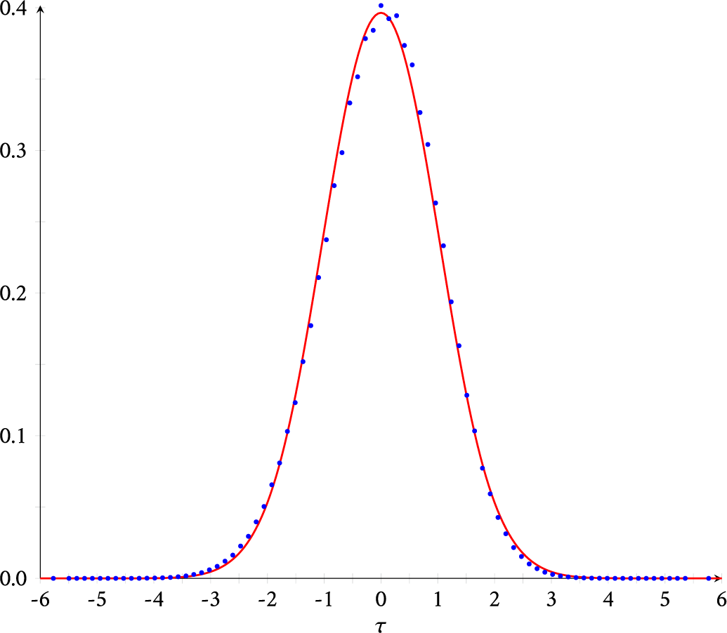
Figure 4: Data for non-hyperelliptic curves of genus $3$ over $\mathbb {F}_q$ for $q=53$ . The blue dots are the points $(t/\sqrt {q},\sqrt {q}\,\mathcal {N}_{q,3}(t/\sqrt {q}))$ for integers $t\in [-42,42]$ . The red curve is the function ${\mathfrak {f}}_3(\tau )$ .

5 The non-hyperelliptic case: experiments and conjectures

We consider now the case of non-hyperelliptic curves of genus $g=3$ . For this purpose, for $g\geq 3$ , we introduce the function $\mathcal {N}^{\text {nhyp}}_{q,g}(\tau )$ , which we define analogously to how we defined $\mathcal {N}_{q,g}(\tau )$ and $\mathcal {N}^{\text {hyp}}_{q,g}(\tau )$ :

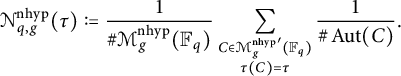
Here, by $\mathcal {M}^{\text {nhyp}}_g(\mathbb {F}_q)$ , we mean the set of $\overline {\mathbb {F}}_q$ -isomorphism classes of non-hyperelliptic curves of genus g over $\mathbb {F}_q$ , and by ${\mathcal {M}^{\text {nhyp}}_g}'(\mathbb {F}_q)$ , we mean the set of $\mathbb {F}_q$ -isomorphism classes of such curves. The associated measures will still weakly converge to the measure $\mu _g$ with density ${\mathfrak {f}}_g$ . But experimentally, the behavior looks much smoother than in the elliptic or hyperelliptic cases as illustrated by Figure 4 for $g=3$ and $q=53$ . ⁴ Note that a similar behavior would certainly hold considering all curves of genus $3$ . Heuristically, these patterns could be understood as an averaging for a given trace over several isogeny classes, but this idea does not work for the hyperelliptic locus as we have seen in Section 4 and something more is needed for a family of curves to “behave nicely.” Still, the experimental data in genus $3$ lead us to state the following conjecture.

Conjecture 5.1 Let $g \geq 3$ . For all $\tau \in I_g$ , for all $\varepsilon>0$ , and for all large enough q, there exists $t\in \mathbb {N}$ such that $\lvert \tau -t/\sqrt {q}\rvert <1/(2\sqrt {q})$ and $\lvert \sqrt {q} \cdot \mathcal {N}^{\text {nhyp}}_{q,g}(t/\sqrt {q})- {\mathfrak {f}}_g(t/\sqrt {q})\rvert <\varepsilon $ .

Another way to phrase this conjecture is to replace the measure $\mu _{q,g}$ by a measure with density given by the histogram with height $\sqrt {q} \cdot \mathcal {N}^{\text {nhyp}}_{q,g}(t/\sqrt {q})$ and base centered at $t/\sqrt {q}$ of length $1/\sqrt {q}$ for all $t\in [-2g \sqrt {q},2g \sqrt {q}]$ . The conjecture asserts that the densities of these measures converge to the density ${\mathfrak {f}}_g$ at each point of $I_g$ . This is stronger than weak convergence of the measures [Sch47].

We now conclude by looking at the symmetry breaking for the trace distribution of (non-hyperelliptic) genus 3 curves. In general, if C is a hyperelliptic curve of genus g over $\mathbb {F}_q$ with trace t, then its quadratic twist for the hyperelliptic involution has trace $-t$ and therefore the distribution of the number of hyperelliptic curves of genus g over $\mathbb {F}_q$ as a function of their trace is symmetric. For non-hyperelliptic curves, the distribution has no reason to be symmetric anymore. Actually, if a principally polarized abelian variety over $\mathbb {F}_q$ is the Jacobian (over $\mathbb {F}_q$ ) of a non-hyperelliptic curve, then its quadratic twist is never a Jacobian. This obstruction, known as Serre’s obstruction, is a huge obstacle to finding a closed formula for the maximal number of rational points for $g=3$ [Lau02], whereas such formulas are known for $g=1$ [Deu41] and $g=2$ [Ser83]. Although we cannot improve on the state-of-the-art of this question, we can study this asymmetry with the probabilistic angle and the results we got before.

To visualize this asymmetry, let us consider the signed measure $\nu _{q,g} = \mu _{q,g} - (-1)^* \mu _{q,g}$ where $(-1)^* \mu _{q,g}$ is the discrete image signed measure defined by

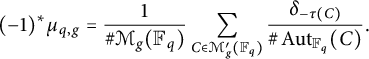$$\begin{align*}(-1)^* \mu_{q,g} =\frac{1}{\# \mathcal{M}_g(\mathbb{F}_q)} \sum_{C\in \mathcal{M}_g'(\mathbb{F}_q)} \frac{\delta_{-\tau(C)}}{\#\operatorname{\mathrm{Aut}}_{\mathbb{F}_q}(C)}.\end{align*}$$

We get the following consequence of Theorem 2.1.

Proposition 5.2 The sequence of signed measures $(\nu _{q,g})$ weakly converges to the $0$ measure.

Proof By definition, the even moments of $\nu _{q,g}$ are zero. By Theorem 2.1, the odd moments of $\sqrt {q}\, \nu _{q,g}$ are equal to

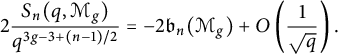$$\begin{align*}2 \frac{S_n(q,\mathcal{M}_g)}{q^{3g-3+(n-1)/2}} = -2 \mathfrak{b}_n(\mathcal{M}_g) + O\left(\frac{1}{\sqrt{q}}\right). \end{align*}$$

Hence, all moments of $\nu _{q,g}$ are $0$ . Now, if f is any continuous function on the compact interval $I_g=[-2g,2g]$ , then by the Stone–Weierstrass theorem, for every $\varepsilon>0$ , we can find a polynomial P such that $\lvert f(\tau )-P(\tau )\rvert \leq \varepsilon $ for all $\tau \in I_g$ . Therefore, we have

$$\begin{align*}\biggl\lvert \int_{I_g} f \,d\nu_{q,g} \biggr\rvert \leq \biggl\lvert\int_{I_g} (f-P) \,d\nu_{q,g} + \int_{I_g} P \,d\nu_{q,g}\biggr\rvert \leq \varepsilon \|\nu_{q,g}\| + \biggl\lvert \int_{I_g} P \,d\nu_{q,g}\biggr\rvert.\end{align*}$$

The last term is a sum of moments which converges to $0$ when q goes to infinity. The variation of $\nu _{g,q}$ is also uniformly bounded since

$$\begin{align*}\|\nu_{q,g}\| = \lvert\nu_{q,g}\rvert(I_g)=\sum_{\tau} \,\Bigl\lvert\mathcal{N}_{q,g}(\tau)-\mathcal{N}_{q,g}(-\tau)\Bigr\rvert \leq 2 \sum_{\tau} \mathcal{N}_{q,g}(\tau) = 2 \mu_{q,g}(I_g)=2.\end{align*}$$

Having a $0$ measure is not very interesting, and the proof of Proposition 5.2 shows that it would be much more interesting to study the weak convergence of the sequence of signed measures $(\sqrt {q} \,\nu _{q,g})$ . We have from the previous proof the following corollary.

Corollary 5.3 The even moments of $\sqrt {q} \,\nu _{q,g}$ are zero, and the odd nth moments of the sequence $(\sqrt {q}\, \nu _{q,g})$ converge to $-2 \mathfrak {b}_n(\mathcal {M}_g)$ .

Unfortunately, we cannot prove weak convergence: The rest of the proof fails as we do not know if one can bound $\sqrt {q}\, \|\nu _{q,g}\|$ uniformly in q (which is a necessary condition for weak convergence). Moreover, one cannot expect a general result from the convergence of moments alone as in the case of (positive) measures as the following counterexample shows.

Example 5.4 Consider the sequence of signed measures $(\mu _i)$ with density $i \sin i x$ on the interval $[0, 2\pi ]$ . The sequence of nth moments converges to $-(2\pi )^n$ which is the nth moment of the signed measure $\mu =-\delta _{2 \pi }$ . But $\|\mu _i\|=4i$ , which is not bounded and therefore the sequence $(\mu _i)$ does not weakly converge (to $\mu $ ) (see, for instance, [Bog18, Proposition 1.4.7]).

Recall from (3.3) that the nth moment of the function

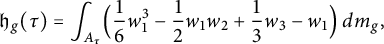$$\begin{align*}{\mathfrak{h}}_g(\tau)=\int_{A_{\tau}} \Bigl(\frac{1}{6}w_1^3-\frac{1}{2}w_1w_2+\frac{1}{3}w_3-w_1 \Bigr)\, d m_g, \end{align*}$$

with $A_{\tau }=\{(\theta _1,\dots ,\theta _g)\in [0,\pi ]^g:\,\sum _{j}2\cos \theta _j= \tau \}$ , is equal to $\mathfrak {b}_n(\mathcal {M}_g)$ . Because of the convergence of the moments above, we conjecture the following.

Conjecture 5.5 For $g \geq 3$ , the sequence of signed measures $(\sqrt {q} \,\nu _{q,g})$ weakly converges to the continuous signed measure with density $-2 {\mathfrak {h}}_g$ .

Such a result would, for instance, imply that $\sqrt {q}\, \|\nu _{q,g}\|$ is uniformly bounded; hence, there exists a constant $C>0$ such that for all q and all $\tau =t/\sqrt {q}$ , we have $\lvert \mathcal {N}_{q,g}(\tau )-\mathcal {N}_{q,g}(-\tau )\rvert \leq C/\sqrt {q}$ .

In genus $3$ , in the same spirit as in Section 4, one can run experiments which illustrate how the values

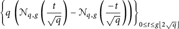$$\begin{align*}\left\{q \, \left(\mathcal{N}_{q,g}\left(\frac{t}{\sqrt{q}}\right)-\mathcal{N}_{q,g}\left(\frac{-t}{\sqrt{q}}\right)\right)\right\}_{0 \leq t \leq g \lfloor 2 \sqrt{q}\rfloor} \end{align*}$$

are close to the values $-2{\mathfrak {h}}_3(t/\sqrt {q})$ . See, for instance, Figure 5 for $q=53$ . Seeing the data, one may even wonder if something stronger would hold in the same line as Conjecture 5.1, at least for $g=3$ .

Under this conjecture, one can use the moments of the density function ${\mathfrak {h}}_3$ to revisit the result of [LRR⁺19]. Based on results of [BDFL10], the authors gave a heuristic explanation for the distribution of the points

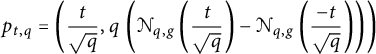$$\begin{align*}p_{t,q}=\left(\frac{t}{\sqrt{q}},q \, \left(\mathcal{N}_{q,g}\left(\frac{t}{\sqrt{q}}\right)-\mathcal{N}_{q,g}\left(\frac{-t}{\sqrt{q}}\right)\right)\right) \end{align*}$$

when $0 \leq t \leq g \lfloor 2\sqrt {q}\rfloor $ by comparing it with the distribution of differences around the mean in the binomial law [LRR⁺19, Corollary 2.3]. With the arguments given there, the distribution is approximated by the function

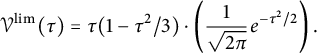$$\begin{align*}\mathcal{V}^{\lim}(\tau) = \tau (1-\tau^2/3) \cdot \left(\frac{1}{\sqrt{2\pi}} e^{-\tau^2 / 2}\right). \end{align*}$$

Graphically, for $q=53$ , the comparison looks acceptable but not perfect (see Figure 5). This is fair as the heuristic grew from a result true when the degree of the plane curves in play is larger than $2q-1$ . As presently we are dealing with non-hyperelliptic curves of genus $3$ , represented as plane curves of degree $4$ , the condition is obviously never fulfilled. It is therefore already stunning that a close, albeit imperfect, match was found in this way.

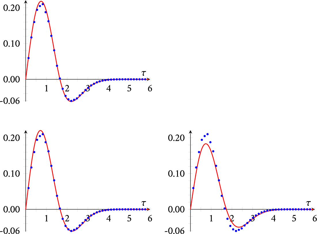
Figure 5: Comparison of genus- $3$ data for $q = 53$ with theoretical approximations. In each graph, the blue dots are the points $\left \{\left (\tau ,q \, \left (\mathcal {N}_{53,3}\left (\tau \right )-\mathcal {N}_{53,3}\left (-\tau \right )\right )\right )\right \}$ with $\tau =t/\sqrt {53}$ and $0 \leq t \leq 42$ . The upper-left graph shows $-2{\mathfrak {h}}_3$ in red. The bottom-left graph shows $\nu ^{\lim }$ in red. The bottom-right graph shows $\mathcal {V}^{\lim }$ in red.

We now take a different road based on Conjecture 5.5 and approximate the density $-2{\mathfrak {h}}_3$ by a function $\nu ^{\lim }$ using the moments $\mathfrak {b}_n(\mathcal {M}_3)$ . By Theorem 2.1, they can be efficiently computed using any symmetric polynomial package. We used Maple and the package SF [Ste95] to compute $\mathfrak {b}_{n}(\mathcal {M}_3)$ for $n=1,3,5,\ldots ,25$ , and found the following values:

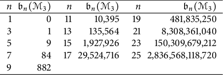
Taking $\nu ^{\lim }(\tau )$ of the form $P(\tau ) \left (\frac {1}{\sqrt {2 \pi }} e^{-\tau ^2/2}\right )$ with P an odd polynomial of degree $5$ , we want

$$\begin{align*}\int_{\mathbb{R}} \tau^{2n+1} \cdot \nu^{\lim}(\tau) \,d\tau = -2 \mathfrak{b}_{2 n+1}(\mathcal{M}_3), \end{align*}$$

for $n=0,1$ , and $2$ , and one finds that

$$\begin{align*}\nu^{\lim}(\tau)= \left(1/60\, \tau^5-1/2\, \tau^3+5/4\, \tau\right) \left(\frac{1}{\sqrt{2 \pi}} e^{-\tau^2/2}\right). \end{align*}$$

Remarkably, the moments of $\nu ^{\lim }(\tau )$ still agree with $-2 \mathfrak {b}_{2n+1}(\mathcal {M}_3)$ for $n=3,4$ , and $5$ . However, for $n=6$ , we find that $\int _{\mathbb {R}}\tau ^{13} \cdot \nu ^{\lim }(\tau )\, d\tau = -2 \cdot 135135 \ne -2 \cdot \mathfrak {b}_{13}(\mathcal {M}_3)$ .

In Figure 5, we see a comparison between the graph of points $\{p_{t,53}\}_{0 \leq t \leq 42}$ and the functions $\mathcal {V}^{\lim }(\tau )$ and $\nu ^{\lim }(\tau )$ , in favor of the latter.