


1 Introduction
The study of N-body problems over curved spaces has its origins in the works of Bolyai [Reference Bolyai4] and Lobachevsky, on the theory of parallels, published in German in 1849 (see part of this work translated into English and published over a century later in [Reference Lobachevsky9]). In [Reference Serret11], the gravitational potential is extended to the sphere
 $\mathbb {S}^2$
, where the potential obtained is of cotangent type. Using the cotangent potential leads to some nonintuitive behavior at a physical level, since it corresponds to a potential defined for a sphere without a point, namely, the punctured sphere
$\mathbb {S}^2$
, where the potential obtained is of cotangent type. Using the cotangent potential leads to some nonintuitive behavior at a physical level, since it corresponds to a potential defined for a sphere without a point, namely, the punctured sphere
 $\mathbb {S}_p^2$
, which gives rise to antipodal singularities (see, e.g., [Reference Boatto, Dritschel and Schaefer2]).
$\mathbb {S}_p^2$
, which gives rise to antipodal singularities (see, e.g., [Reference Boatto, Dritschel and Schaefer2]).
This paper considers the potential derived by considering the unit sphere from an intrinsic geometry point of view and using the Hodge decomposition theorem to derive the central force extension to the various surfaces of interest. In the case of the sphere, the resulting potential is a logarithmic one and it is defined over the entire sphere
 $\mathbb {S}^2$
. For more details, see [Reference Andrade, Boatto, Combot, Duarte and Stuchi1, Reference Boatto, Dritschel and Schaefer2]. Additionally, the corresponding Hodge potential for closed hyper-surfaces is derived by Dritschel in [Reference Dritschel5].
$\mathbb {S}^2$
. For more details, see [Reference Andrade, Boatto, Combot, Duarte and Stuchi1, Reference Boatto, Dritschel and Schaefer2]. Additionally, the corresponding Hodge potential for closed hyper-surfaces is derived by Dritschel in [Reference Dritschel5].
Thus, for the unit sphere
 $\mathbb {S}^2$
, a system of N masses
$\mathbb {S}^2$
, a system of N masses
 $m_1,m_2,\ldots ,m_N$
with positions
$m_1,m_2,\ldots ,m_N$
with positions
 $r_1,r_2,\ldots ,r_N$
, respectively, where
$r_1,r_2,\ldots ,r_N$
, respectively, where
 $r_j = (\varphi _j,\theta _j)$
(with
$r_j = (\varphi _j,\theta _j)$
(with
 $\varphi _j$
the longitude and
$\varphi _j$
the longitude and
 $\theta _j$
the co-latitude), the potential energy of the system is a function
$\theta _j$
the co-latitude), the potential energy of the system is a function
 $U(r)$
, with
$U(r)$
, with
 $$ \begin{align} U(r) = \gamma \sum_{j=1}^N\sum_{k>j}^N m_jm_k \ln(1 - d_{jk}), \end{align} $$
where
 $r = (r_1,r_2,\ldots ,r_N)$
,
$r = (r_1,r_2,\ldots ,r_N)$
,
 $d_{jk}= \cos \theta _j \cos \theta _k + \sin \theta _j \sin \theta _k \cos (\varphi _j -\varphi _k)$
and
$d_{jk}= \cos \theta _j \cos \theta _k + \sin \theta _j \sin \theta _k \cos (\varphi _j -\varphi _k)$
and
 $\gamma $
is the gravitational constant.
$\gamma $
is the gravitational constant.
We will focus on the analysis of stability of a ring of bodies lying on a fixed parallel and rotating uniformly with respect to the z-axis. For this purpose, we consider N bodies with identical masses
 $m_1=\cdots = m_N = 1$
in the Hamiltonian system associated with the potential (1.1). We will show that the regular N-gon configuration is a solution with position
$m_1=\cdots = m_N = 1$
in the Hamiltonian system associated with the potential (1.1). We will show that the regular N-gon configuration is a solution with position
 $\varphi _j = \nu t + \phi _j$
,
$\varphi _j = \nu t + \phi _j$
,
 $\phi _j= \frac {2\pi (j-1)}{N}$
,
$\phi _j= \frac {2\pi (j-1)}{N}$
,
 $\theta _j=\theta _0\in (0,\pi )$
, for
$\theta _j=\theta _0\in (0,\pi )$
, for
 $j=1,\ldots ,N$
and
$j=1,\ldots ,N$
and
 $\nu \neq 0$
, if and only if, the angular velocity is taken as
$\nu \neq 0$
, if and only if, the angular velocity is taken as
 $$\begin{align*}\nu=\frac{\sqrt{N-1}}{\sin\theta_0}.\end{align*}$$
In addition to the aforementioned articles, we can find more recent works in which similar problems defined in curved surfaces are studied for both the N-vortex problem and the N-body problem. The linear stability of a ring-poles configuration with total vorticity equal to zero is studied in [Reference Boatto and Simó3], whereas the linear stability of a ring solution in an infinite cylinder is studied in [Reference Andrade, Boatto, Combot, Duarte and Stuchi1]. Furthermore, the problem of determining the stability of a ring of bodies in the sphere
 $\mathbb {S}^2$
with a cotangent potential has been recently studied in [Reference Hernández-Garduño, Pérez-Chavela and Zhu8], obtaining results about spectral instability for a ring close to the poles and close to the equator. For logarithmic potential, this problem has not been studied previously and it will be totally characterized in this paper.
$\mathbb {S}^2$
with a cotangent potential has been recently studied in [Reference Hernández-Garduño, Pérez-Chavela and Zhu8], obtaining results about spectral instability for a ring close to the poles and close to the equator. For logarithmic potential, this problem has not been studied previously and it will be totally characterized in this paper.
1.1 Equations of motion
We consider a system of N masses
 $m_1, m_2,\ldots ,m_N$
with positions
$m_1, m_2,\ldots ,m_N$
with positions
 $r_1, r_2,\ldots ,r_N$
, respectively, where
$r_1, r_2,\ldots ,r_N$
, respectively, where
 $r_j = (\varphi _j,\theta _j)$
(with
$r_j = (\varphi _j,\theta _j)$
(with
 $\varphi _j$
the longitude and
$\varphi _j$
the longitude and
 $\theta _j$
the co-latitude). The potential energy of the system is the function
$\theta _j$
the co-latitude). The potential energy of the system is the function
 $U(r)$
, where
$U(r)$
, where
 $r = (r_1, r_2,\ldots ,r_N)$
and
$r = (r_1, r_2,\ldots ,r_N)$
and
 $U(r)$
is the potential energy obtained in [Reference Boatto, Dritschel and Schaefer2] and given in (1.1). On the other hand, if
$U(r)$
is the potential energy obtained in [Reference Boatto, Dritschel and Schaefer2] and given in (1.1). On the other hand, if
 $v_1, v_2,\ldots ,v_N$
are the velocity vectors, then the kinetic energy is defined by
$v_1, v_2,\ldots ,v_N$
are the velocity vectors, then the kinetic energy is defined by
 $$ \begin{align} \mathcal{K}=\frac{1}{2}\sum_{j=1}^Nm_jv_j^Tg_jv_j, \end{align} $$
where g is the metric tensor
 $$ \begin{align} g_j=\left( \begin{array}{cc} \sin^2\theta_j & 0 \\ 0 & 1 \\ \end{array} \right). \end{align} $$
Thus, the Lagrangian of the system is
 $\mathcal {L} = \mathcal {K} - U$
and the Legendre transformation allows to write the velocities in terms of the momentum
$\mathcal {L} = \mathcal {K} - U$
and the Legendre transformation allows to write the velocities in terms of the momentum
 $p_j = (p_{\varphi _j}, p_{\theta _j})$
. In fact,
$p_j = (p_{\varphi _j}, p_{\theta _j})$
. In fact,
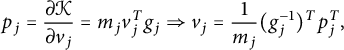 $$\begin{align*}p_j =\frac{\partial\mathcal{K}}{\partial v_j} = m_jv_j^Tg_j\Rightarrow v_j =\frac{1}{m_j}(g_j^{-1})^Tp^T_j,\end{align*}$$
and the kinetic energy in terms of the momentum takes the form
 $$ \begin{align} \mathcal{K}=\sum_{j=1}^N\frac{1}{2m_j}p_j(g_j^{-1})^Tp^T_j=\sum_{j=1}^N\frac{1}{2m_j}(p_{\varphi_j}^2\csc^2\theta_j+p_{\theta_j}^2). \end{align} $$
The Hamiltonian function is given by
 $$ \begin{align} H(Q,P) = \mathcal{K}(Q, P) + U(Q), \end{align} $$
with
 $Q = (r_1, r_2,\ldots , r_N )$
and
$Q = (r_1, r_2,\ldots , r_N )$
and
 $P = (p_1,p_2,\ldots , p_N)$
. Thus, the corresponding Hamiltonian equations take the form
$P = (p_1,p_2,\ldots , p_N)$
. Thus, the corresponding Hamiltonian equations take the form
 $$ \begin{align} \begin{split} \dot{\varphi}_j & = \frac{\partial H}{\partial p_{\varphi_j}}= \frac{1}{m_j}\csc^2\theta_jp_{\varphi_j}, \\ \dot{\theta}_j & = \frac{\partial H}{\partial p_{\theta_j}}= \frac{1}{m_j}p_{\theta_j}, \\ \dot{p}_{\varphi_j} & = -\frac{\partial H}{\partial\varphi_j}= -\gamma\sum_{k=1,k\neq j}^{N}\frac{m_jm_k\sin\theta_j\sin\theta_k\sin(\varphi_j-\varphi_k)}{1-d_{jk}}, \\ \dot{p}_{\theta_j} & = -\frac{\partial H}{\partial \theta_j}= \frac{1}{m_j}\cot\theta_j\csc^2\theta_jp_{\varphi_j}^2\\ &\quad -\gamma\sum_{k=1,k\neq j}^{N}\frac{m_jm_k\left(\cos\theta_k\sin\theta_j-\cos\theta_j\sin\theta_k\cos(\varphi_j-\varphi_k)\right)}{1-d_{jk}}. \end{split} \end{align} $$
1.2 Symmetries
The Hamiltonian (1.5) is invariant under the action of
 $SO(3)$
, in particular, by rotations of
$SO(3)$
, in particular, by rotations of
 $SO(2)$
about the z-axis, which implies the conservation of the total
$SO(2)$
about the z-axis, which implies the conservation of the total
 $\varphi $
component of the angular momentum
$\varphi $
component of the angular momentum
 $P_{\varphi }=\sum p_{\varphi _j}$
. Additionally, it is easy to see that the Hamiltonian function (1.5) also has the translation time-dependent symmetry
$P_{\varphi }=\sum p_{\varphi _j}$
. Additionally, it is easy to see that the Hamiltonian function (1.5) also has the translation time-dependent symmetry
 $\varphi _j\mapsto \varphi _j+v t$
.
$\varphi _j\mapsto \varphi _j+v t$
.
1.3 Ring solution
Let us consider a system of N bodies with identical masses
 $m_1 = \cdots = m_N = m$
. By this assumption, the Hamiltonian function becomes simpler. Moreover, we may assume without lost of generality that
$m_1 = \cdots = m_N = m$
. By this assumption, the Hamiltonian function becomes simpler. Moreover, we may assume without lost of generality that
 $m = \gamma = 1$
. Indeed, it is achieved by introducing the
$m = \gamma = 1$
. Indeed, it is achieved by introducing the
 $\left (\frac {1}{c}\right )-$
symplectic change of coordinates
$\left (\frac {1}{c}\right )-$
symplectic change of coordinates
 $(Q,P)\mapsto (Q, c P)$
and the scaling
$(Q,P)\mapsto (Q, c P)$
and the scaling
 $x\mapsto \frac {m}{c}x$
in time and energy, with
$x\mapsto \frac {m}{c}x$
in time and energy, with
 $c=\gamma ^{1/2}m^{3/2}$
. Thus, we arrive to the Hamiltonian function
$c=\gamma ^{1/2}m^{3/2}$
. Thus, we arrive to the Hamiltonian function
 $$ \begin{align} \mathcal{H}=\sum_{j=1}^N\frac{1}{2}(p_{\varphi_j}^2\csc^2\theta_j+p_{\theta_j}^2)+\sum_{j=1}^N\sum_{k>j}^N\ln(1-d_{jk}). \end{align} $$
Now, we consider a polygonal configuration formed by N identical masses placed at the vertices of a regular polygon, rotating with respect to its normal vector with constant angular velocity. Due to the
 $SO(3)$
-symmetry, we can consider without loss of generality that the polygon is rotating in a fixed latitude around the z-axis. Such a particular configuration must be of the form
$SO(3)$
-symmetry, we can consider without loss of generality that the polygon is rotating in a fixed latitude around the z-axis. Such a particular configuration must be of the form
 $$ \begin{align} \varphi_j = \nu t + \phi_j,\quad \theta_j = \theta_0\in(0, \pi),\quad p_{\varphi_j} = \nu\sin^2\theta_0,\quad p_{\theta_j}=0, \end{align} $$
where
 $\phi _j = \frac {2\pi (j-1)}{N}$
and
$\phi _j = \frac {2\pi (j-1)}{N}$
and
 $\nu $
is the constant angular velocity. It is verified that if
$\nu $
is the constant angular velocity. It is verified that if
 $\theta _0\neq \frac {\pi }{2}$
, then the configuration (1.8) will be a relative equilibrium of the system associated with (1.7), if and only if the angular velocity satisfies
$\theta _0\neq \frac {\pi }{2}$
, then the configuration (1.8) will be a relative equilibrium of the system associated with (1.7), if and only if the angular velocity satisfies
 $$ \begin{align} \nu^2 = \frac{N - 1}{\sin^2\theta_0}. \end{align} $$
For
 $\theta _0=\frac {\pi }{2}$
, the formula (1.9) is no longer valid and we get the nonisolated solution
$\theta _0=\frac {\pi }{2}$
, the formula (1.9) is no longer valid and we get the nonisolated solution
 $$ \begin{align} \varphi_j=p_{\varphi} t + \phi_j, \quad \theta_j=\frac{\pi}{2},\quad \quad p_{\varphi_j} = p_{\varphi}, \quad p_{\theta_j}=0. \end{align} $$
The structure of this work is as follows. In Section 1, we describe the equations of motion for the
 $ N$
-body problem over the entire sphere
$ N$
-body problem over the entire sphere
 $ \mathbb {S}^2 $
and for identical masses
$ \mathbb {S}^2 $
and for identical masses
 $m_1=\cdots =m_N$
, we can find a particular solution called ring solution. In Section 2, the spectral stability of the ring solution of the complete problem is studied, obtaining spectral stability for
$m_1=\cdots =m_N$
, we can find a particular solution called ring solution. In Section 2, the spectral stability of the ring solution of the complete problem is studied, obtaining spectral stability for
 $ 2 \leq N \leq 6 $
and spectral instability for
$ 2 \leq N \leq 6 $
and spectral instability for
 $ N \geq 7 $
. In Section 3, on the space of homothetic solutions, we reduce the system to two and one degrees of freedom, respectively. Additionally, we calculate the equilibrium solutions of both reduced systems and study the phase portraits near the equilibria of the reduced system with one degree of freedom. To examine the stability of the ring solution, we normalize the Hamiltonian to terms of degree three via the Lie algorithm, and we determine that the ring solution is unstable in the Lyapunov sense. Finally, in Section 4, we give conditions for the existence of periodic orbits in the complete system along with some examples.
$ N \geq 7 $
. In Section 3, on the space of homothetic solutions, we reduce the system to two and one degrees of freedom, respectively. Additionally, we calculate the equilibrium solutions of both reduced systems and study the phase portraits near the equilibria of the reduced system with one degree of freedom. To examine the stability of the ring solution, we normalize the Hamiltonian to terms of degree three via the Lie algorithm, and we determine that the ring solution is unstable in the Lyapunov sense. Finally, in Section 4, we give conditions for the existence of periodic orbits in the complete system along with some examples.
2 Spectral stability of the ring solution
From now on, we move to a co-rotating frame associated with the solution (1.8) (
 $\theta _0\neq \pi /2$
). Hence, it becomes a fixed equilibrium of the new Hamiltonian system. To analyze the spectral stability of the ring solution, we compute the Hessian matrix evaluated at the solution (1.8)
$\theta _0\neq \pi /2$
). Hence, it becomes a fixed equilibrium of the new Hamiltonian system. To analyze the spectral stability of the ring solution, we compute the Hessian matrix evaluated at the solution (1.8)
 $$ \begin{align} D_z^2\mathcal{H}(z)=\left( \begin{array}{cccc} S & 0_N & 0_N & 0_N \\ 0_N & R & \alpha I_N & 0_N \\ 0_N & \alpha I_N & \beta I_N & 0_N \\ 0_N & 0_N & 0_N & I_N \\ \end{array} \right), \end{align} $$
where
 $z=(\varphi _1, \ldots , \varphi _N, \theta _1, \ldots , \theta _N, p_{\varphi _1}, \ldots ,p_{\varphi _N}, p_{\theta _1},\ldots , p_{\theta _N})$
,
$z=(\varphi _1, \ldots , \varphi _N, \theta _1, \ldots , \theta _N, p_{\varphi _1}, \ldots ,p_{\varphi _N}, p_{\theta _1},\ldots , p_{\theta _N})$
,
 $\alpha =-2 \nu \cot \theta _0 $
,
$\alpha =-2 \nu \cot \theta _0 $
,
 $\beta =\csc ^2\theta _0 $
,
$\beta =\csc ^2\theta _0 $
,
 $0_N$
, and
$0_N$
, and
 $I_N$
are the zero and identity matrix of order
$I_N$
are the zero and identity matrix of order
 $N\times N$
, respectively, and
$N\times N$
, respectively, and
 $$\begin{align*}S=s I_N + P_N, \quad R=r I_N - \beta P_N,\end{align*}$$
with
 $$\begin{align*}s=-\frac{1}{6}(N^2-1),\quad r=\nu{}^2 \left(2+ \cos 2 \theta _0\right) +\frac{\beta }{6} (N-5) (N-1), \quad P_N=\left(\rho_{ij}\right)_{N\times N},\end{align*}$$
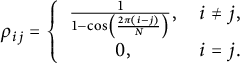 $$\begin{align*}\quad \rho_{ij}=\left\lbrace\begin{array}{cl} \frac{1}{1-\cos\left(\frac{2\pi (i-j)}{N}\right)}, & i\neq j,\\ 0,&i=j.\end{array} \right.\end{align*}$$
The spectral stability of the solution (1.8) is determined through the eigenvalues of the matrix
 $J D^2\mathcal {H}$
, where J is the standard symplectic matrix. The characteristic polynomial is
$J D^2\mathcal {H}$
, where J is the standard symplectic matrix. The characteristic polynomial is
 $$\begin{align*}p(\lambda)=\det [D^2\mathcal{H}+\lambda J] = \beta^N\det\left[-\beta P_N^2+\delta P_N+g(\lambda) I_N\right],\end{align*}$$
where
 $\delta =-{\alpha ^2}/{\beta }+r-\beta s, g(\lambda )={1}{/\beta }\lambda ^4 + \left ({r}/{\beta }+s\right ) \lambda ^2 +r s-{\alpha ^2 s}/{\beta } $
and
$\delta =-{\alpha ^2}/{\beta }+r-\beta s, g(\lambda )={1}{/\beta }\lambda ^4 + \left ({r}/{\beta }+s\right ) \lambda ^2 +r s-{\alpha ^2 s}/{\beta } $
and
 $P_N$
is a circulant matrix
$P_N$
is a circulant matrix
 $$\begin{align*}P_N=\left(\begin{array}{ccccccc} p_1&p_2&p_3&\ldots & p_{N-2} & p_{N-1}&p_N\\ p_N&p_1&p_2&\ldots &p_{N-3}& p_{N-2} & p_{N-1}\\ p_{N-1}&p_N&p_1 &\ldots &p_{N-4}& p_{N-3} & p_{N-2}\\ \vdots & \vdots&\vdots &\ddots &\vdots & \vdots&\vdots\\ p_2 &p_3&p_4&\ldots & p_3&p_2&p_1 \end{array}\right):=Circ\left[p_1,p_2, \ldots,p_N\right],\end{align*}$$
with
 $p_1=0 \mbox { and } p_k=\rho _{k1},\, k=2, \ldots , N$
. Furthermore, taking into account the following relation:
$p_1=0 \mbox { and } p_k=\rho _{k1},\, k=2, \ldots , N$
. Furthermore, taking into account the following relation:
 $$ \begin{align} p_{j}=p_{N-j+2}, \qquad j=2,\ldots, N, \end{align} $$
we have that
 $P_N$
is a symmetric circulant matrix. Therefore, the matrix
$P_N$
is a symmetric circulant matrix. Therefore, the matrix
 $\Lambda _N:=-\beta P_N^2+\delta P_N+g(\lambda ) I_N$
is also symmetric circulant, i.e.,
$\Lambda _N:=-\beta P_N^2+\delta P_N+g(\lambda ) I_N$
is also symmetric circulant, i.e.,
 $$\begin{align*}\Lambda_N:=Circ\left[x_1,x_2, \ldots,x_N\right], \mbox{ with } x_{j}=x_{N-j+2}, \,\, j=2,\ldots, N.\end{align*}$$
Thus, ignoring the constant factor
 $\beta ^N$
, we get the characteristic polynomial
$\beta ^N$
, we get the characteristic polynomial
 $$ \begin{align} p(\lambda)=\det\Lambda_N=\displaystyle\prod_{j=1}^N\left(x_1+x_2\omega_j+x_3\omega_j^2+\cdots +x_N\omega_j^{N-1}\right), \end{align} $$
where
 $\omega _j$
is the jth root of unity. The eigenvalues of the matrix
$\omega _j$
is the jth root of unity. The eigenvalues of the matrix
 $P_N$
are given by
$P_N$
are given by
 $$\begin{align*}\tau_j=p_1+p_2\omega_j+p_3\omega_j^2+\cdots +p_N\omega_j^{N-1}, j=1, \ldots, N,\end{align*}$$
and denoting
 $P_N^2=Circ\left [q_1, q_2, \ldots , q_N\right ]$
, it is verified that the eigenvalues of
$P_N^2=Circ\left [q_1, q_2, \ldots , q_N\right ]$
, it is verified that the eigenvalues of
 $P_N^2$
are given by
$P_N^2$
are given by
 $$\begin{align*}\sigma_j=q_1+q_2\omega_j+q_3\omega_j^2+\cdots +q_N\omega_j^{N-1}=\tau_j^2.\end{align*}$$
See [Reference Gelfand and Shenitzer6] for more details about circulant matrices results. Now, from the definition of
 $\Lambda _N$
it follows that
$\Lambda _N$
it follows that
 $$ \begin{align} x_1=-\beta q_1+g(\lambda), \mbox{ and } x_k=-\beta q_k+\delta p_k, \quad k=2,\ldots, N. \end{align} $$
By replacing the quantities (2.4) into (2.3), we arrive at
 $$ \begin{align} p(\lambda)=\displaystyle\prod_{j=1}^N\left(g(\lambda) +\delta \tau_j-\beta \tau_j^2\right). \end{align} $$
Note that from condition (2.2), using the fact that
 $\omega _j^{N-k+1}=\overline {\omega }_j^{k-1}$
and in virtue of the formula given in [Reference Hansen7, p. 271], we obtain an explicit expression for the eigenvalues of
$\omega _j^{N-k+1}=\overline {\omega }_j^{k-1}$
and in virtue of the formula given in [Reference Hansen7, p. 271], we obtain an explicit expression for the eigenvalues of
 $P_N$
, namely
$P_N$
, namely
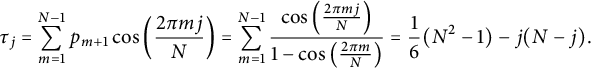 $$\begin{align*}\tau_j=\sum_{m=1}^{N-1}p_{m+1}\cos\left(\frac{2\pi mj}{N}\right)=\sum_{m=1}^{N-1}\frac{\cos\left(\frac{2\pi mj}{N}\right)}{1-\cos\left(\frac{2\pi m}{N}\right)}=\frac{1}{6}(N^2-1)-j(N-j).\end{align*}$$
Thus, we obtain that the
 $4N$
eigenvalues read as follows:
$4N$
eigenvalues read as follows:
 $$ \begin{align} \lambda_{1j}=\frac{1}{\sqrt{2}}\sqrt{a+\sqrt{b_j}},\,\, \lambda_{2j}=\frac{1}{\sqrt{2}}\sqrt{a-\sqrt{b_j}},\,\, \lambda_{3j}=-\lambda_{1j}, \,\, \lambda_{4j}=-\lambda_{2j}, \end{align} $$
with
 $j=1, \ldots , N,$
and
$j=1, \ldots , N,$
and
 $$ \begin{align} \begin{array}{rl} a =& -r-s\beta, \\ b_j=& 4 \alpha ^2 s+(r-\beta s)^2+4\tau _j \left(\alpha ^2+\beta ^2 \tau _j-\beta r+\beta ^2 s\right).\\ \end{array} \end{align} $$
By replacing the expressions
 $r,s,\alpha ,\beta ,\tau _j$
in terms of
$r,s,\alpha ,\beta ,\tau _j$
in terms of
 $\theta _0, N$
, and j, we obtain
$\theta _0, N$
, and j, we obtain
 $$\begin{align*}\lambda_{1j}=\sqrt{-(j-1) (j-N+1)-(N-1) \cos 2 \theta_0 }\csc \theta_0, \quad \lambda_{2j}=i\sqrt{j (N-j)}\csc \theta_0, \end{align*}$$
where we observe the following properties:
-
(i)
 $\lambda _{2j}\in i\mathbb {R}$
, for all
$j=1, \ldots , N-1$
.
$\lambda _{2j}\in i\mathbb {R}$
, for all
$j=1, \ldots , N-1$
. -
(ii)
$\lambda _{2N}=0$
. -
(iii)
$\lambda _{pj}=\lambda _{p,N-j}$
for all
$j=1, \ldots , \lfloor \frac {N-1}{2} \rfloor $
,
$p=1,2$
.


Note that property (iii) implies that for N even,
 $\pm \lambda _{p,\frac {N}{2}}, \pm \lambda _{1N}$
are the only eigenvalues with multiplicity one, while the remaining
$\pm \lambda _{p,\frac {N}{2}}, \pm \lambda _{1N}$
are the only eigenvalues with multiplicity one, while the remaining
 $4N-6$
eigenvalues have multiplicity two. For N odd,
$4N-6$
eigenvalues have multiplicity two. For N odd,
 $\pm \lambda _{1N}$
are the only eigenvalues with multiplicity one, while the remaining
$\pm \lambda _{1N}$
are the only eigenvalues with multiplicity one, while the remaining
 $4N-2$
eigenvalues have multiplicity two.
$4N-2$
eigenvalues have multiplicity two.
Finally, the spectral stability depends on the eigenvalues
 $\lambda _{1N}$
. It is easy to verify that
$\lambda _{1N}$
. It is easy to verify that
 $$\begin{align*}\lambda_{max}:=\sqrt{\max_{j}\lambda_{1j}^2}=\lambda_{1,\lfloor\frac{N}{2}\rfloor}=\left\lbrace\begin{array}{cl} \sqrt{\left(1-\frac{N}{2}\right)^2-(N-1) \cos 2 \theta_0 }\csc \theta_0 , &\mbox{ if }N \mbox{ is even},\\ & \\ \frac{1}{2} \sqrt{(N-1) (N-3 -4 \cos 2 \theta_0 )}\csc \theta_0, &\mbox{ if } N \mbox{ is odd}, \end{array} \right.\end{align*}$$
and it follows that
 $\lambda _{max}^2\leq 0$
, if and only if,
$\lambda _{max}^2\leq 0$
, if and only if,
 $\theta _0\in \left (0,\Theta _N\right ] \cup \left [\pi -\Theta _N,\pi \right )$
with
$\theta _0\in \left (0,\Theta _N\right ] \cup \left [\pi -\Theta _N,\pi \right )$
with
 $$\begin{align*}\Theta_N=\frac{1}{2} \left\lbrace \begin{array}{ll} \arccos\left(\frac{(N-2)^2}{4(N-1)}\right),& \mbox{if N is even,}\\ \arccos\left(\frac{N-3}{4}\right),& \mbox{if N is odd,} \end{array} \right.\end{align*}$$
which is a real number only for
 $2\leq N\leq 6$
.
$2\leq N\leq 6$
.
Therefore, we may conclude the following result.
Theorem 2.1. For
 $2\leq N\leq 6$
, there exists
$2\leq N\leq 6$
, there exists
 $\Theta _N\in (0,\pi )$
such that the ring solution is spectrally stable for any
$\Theta _N\in (0,\pi )$
such that the ring solution is spectrally stable for any
 $\theta _0\in \left (0,\Theta _N\right ) \cup \left (\pi -\Theta _N,\pi \right )$
(see Figure 1) if
$\theta _0\in \left (0,\Theta _N\right ) \cup \left (\pi -\Theta _N,\pi \right )$
(see Figure 1) if
 $N=2, 3$
and any
$N=2, 3$
and any
 $\theta _0\in \left (0,\Theta _N\right ] \cup \left [\pi -\Theta _N,\pi \right )$
if
$\theta _0\in \left (0,\Theta _N\right ] \cup \left [\pi -\Theta _N,\pi \right )$
if
 $N=4,5,6$
. For
$N=4,5,6$
. For
 $N\geq 7$
, the ring solution is unstable at any parallel where the ring is located.
$N\geq 7$
, the ring solution is unstable at any parallel where the ring is located.

Figure 1: Shaded regions correspond to zones of
 $\mathbb {S}^2$
where the ring solution is spectrally stable. These regions exist only for
$\mathbb {S}^2$
where the ring solution is spectrally stable. These regions exist only for
 $2\leq N\leq 6$
.
$2\leq N\leq 6$
.
The stability of the ring placed at the equator must be studied separately. Since the set
 $\theta _1=\cdots =\theta _N=\pi /2$
is an invariant set, we can restrict the system to the equator. The equations of motion restricted to the equator and written in a co-rotating frame are given by the N-d.o.f. Hamiltonian system:
$\theta _1=\cdots =\theta _N=\pi /2$
is an invariant set, we can restrict the system to the equator. The equations of motion restricted to the equator and written in a co-rotating frame are given by the N-d.o.f. Hamiltonian system:
 $$ \begin{align} \begin{split} \dot{\phi}_j & =p_{\phi_j} - \nu, \\\dot{\theta}_j & =0,\\\dot{p}_{\phi_j} & =-\sum_{k=1,k\neq j}^{N}\frac{\sin(\phi_j-\phi_k)}{1-\cos(\phi_j-\phi_k)},\\\dot{p}_{\theta_j} & =0.\\ \end{split} \end{align} $$
Solution (1.10) corresponds to the fixed equilibrium
 $\phi _j=2\pi (j-1)/N$
,
$\phi _j=2\pi (j-1)/N$
,
 $p_{\phi _j}=\nu $
. The matrix of the linearization at this equilibrium is given by
$p_{\phi _j}=\nu $
. The matrix of the linearization at this equilibrium is given by
 $$\begin{align*}\mathcal{A}=\left( \begin{array}{cc} R_N & 0_N \\ 0_N & I_N \\ \end{array} \right), \end{align*}$$
with
 $R_N=s I_N-P_N$
, where s and
$R_N=s I_N-P_N$
, where s and
 $P_N$
are defined in the previous case.
$P_N$
are defined in the previous case.
Similarly to the case
 $\theta _0\neq \pi /2$
, we get the eigenvalues
$\theta _0\neq \pi /2$
, we get the eigenvalues
 $$\begin{align*}\lambda_j=\pm\sqrt{\frac{1}{3}(N^2-1)-j(N-j)}\in \mathbb{R},\, j=1,\ldots,N.\end{align*}$$
Thus, we conclude the following result.
Theorem 2.2. For
 $\theta _0=\pi /2$
and
$\theta _0=\pi /2$
and
 $N\geq 2$
, the ring solution (1.10) is unstable.
$N\geq 2$
, the ring solution (1.10) is unstable.
Remark 2.3 The study stability of the ring relative equilibria for cotangent potential has been recently treated in [Reference Hernández-Garduño, Pérez-Chavela and Zhu8], where the authors prove spectral instability for a ring close to the poles for any
 $N\geq 2$
, which differs with the results obtained in Theorem 2.1 for
$N\geq 2$
, which differs with the results obtained in Theorem 2.1 for
 $2\leq N\leq 6$
.
$2\leq N\leq 6$
.
3 Nonlinear stability of the ring solution in the space of homothetic ring solutions
3.1 Reduction
In order to study the nonlinear stability, we consider identical masses such that at any time they form a regular polygon contained in a plane parallel to the
 $xy$
plane. Thus, we consider solutions with positions given by
$xy$
plane. Thus, we consider solutions with positions given by
 $$ \begin{align} r_j=(\varphi_j,\theta_j)=\left(\varphi+\frac{2(j-1)\pi}{N},\theta\right),\, j=1,\ldots,N. \end{align} $$
By replacing (3.1) into (1.6) with the Hamiltonian given in (1.7), we obtain that
 $\varphi $
is a cyclic variable and the system may be reduced by one degree of freedom:
$\varphi $
is a cyclic variable and the system may be reduced by one degree of freedom:
 $$ \begin{align} \begin{split} \dot{\varphi} & =p_{\varphi}\csc^2\theta, \\ \dot{\theta} & =p_{\theta},\\ \dot{p}_{\varphi} & =0,\\ \dot{p}_{\theta} & =\cot\theta\csc^2\theta p_{\varphi}^2-(N-1)\cot\theta.\\ \end{split} \end{align} $$
Thus, the reduction is carried out by fixing the integral of motion
 $p_{\varphi }=c$
, and the reduced Hamiltonian function read as follows:
$p_{\varphi }=c$
, and the reduced Hamiltonian function read as follows:
 $$ \begin{align} \mathcal{H}_c=\frac{1}{2}(p_{\theta }^2+c^2\csc^2\theta)+(N-1)\ln(\sin\theta), \end{align} $$
with associated Hamiltonian system:
 $$ \begin{align} \begin{split} \dot{\theta} & = p_{\theta },\\ \dot{p}_{\theta} & = c^2\cot\theta\csc^2\theta-(N-1)\cot\theta. \end{split} \end{align} $$
3.2 Equilibria and periodic solutions
The equilibrium points of (3.4) give rise to periodic solutions of the two degrees of freedom system (3.2) of the form
 $$\begin{align*}z(t)=(\nu t+\varphi_0, \theta_0, \nu \sin^2\theta_0, 0),\end{align*}$$
where
 $\nu $
is either a constant depending on
$\nu $
is either a constant depending on
 $(\theta _0,N)$
(for a nonequatorial ring) or an arbitrary value (for an equatorial ring). Furthermore, if
$(\theta _0,N)$
(for a nonequatorial ring) or an arbitrary value (for an equatorial ring). Furthermore, if
 $\theta _0\neq \frac {\pi }{2}$
, then this periodic solution coincides with the ring solution defined in Section 1.3. Such a particular periodic solution can also be obtained as a fixed equilibrium of the system (3.2) provided a co-rotating frame, i.e., by introducing the change of coordinates
$\theta _0\neq \frac {\pi }{2}$
, then this periodic solution coincides with the ring solution defined in Section 1.3. Such a particular periodic solution can also be obtained as a fixed equilibrium of the system (3.2) provided a co-rotating frame, i.e., by introducing the change of coordinates
 $\varphi =\nu t+\phi $
to obtain the new Hamiltonian
$\varphi =\nu t+\phi $
to obtain the new Hamiltonian
 $$ \begin{align} \mathcal{H}=\frac{1}{2}(\csc^2\theta p_{\phi}^2+p_{\theta}^2)-\nu p_{\phi}+(N-1)\ln(\sin\theta), \end{align} $$
with Hamiltonian equations:
 $$ \begin{align} \begin{split} \dot{\phi} & =p_{\phi}\csc^2\theta-\nu, \\ \dot{\theta} & =p_{\theta},\\ \dot{p}_{\phi} & =0,\\ \dot{p}_{\theta} & =\cot\theta \left( p_{\phi}^2 \csc^2\theta -(N-1) \right). \end{split} \end{align} $$
To characterize the equilibria of (3.6), we distinguish the following three cases:
-
(1) General equilibrium:
$\nu>0$
and
$\theta \neq \pi /2$
given by (3.7)
$$ \begin{align} X_0:\,\, \phi=0,\quad\theta=\theta_0\in(0,\pi)\backslash\{\pi/2\},\; p_{\phi}=\sqrt{(N-1)}\sin\theta_0,\;\text{and}\; p_{\theta}=0. \end{align} $$
-
(2) Equatorial equilibrium 1:
$\nu \neq 0$
and
$\theta =\pi /2:$
(3.8)
$$ \begin{align} X_0:\,\, \phi=0,\quad\theta=\theta_0=\pi/2,\quad p_{\phi}=\nu,\;\text{and}\quad p_{\theta}=0. \end{align} $$
-
(3) Equatorial equilibrium 2:
$\nu =0$
: (3.9)
$$ \begin{align} X_0:\,\, \phi=0,\quad\theta=\theta_0=\pi/2,\quad p_{\phi}=0,\quad\text{and}\quad p_{\theta}=0. \end{align} $$


3.3 Dynamics in the reduced
$1$
-d.o.f. system

Notice that the equilibrium points of the
 $1$
-d.o.f. reduced system (3.4) are of the form
$1$
-d.o.f. reduced system (3.4) are of the form
 $(\theta ,0)$
, where
$(\theta ,0)$
, where
 $\theta \in (0,\pi )$
is a zero of the function
$\theta \in (0,\pi )$
is a zero of the function
 $f_c(\theta )=\cot \theta (c^2\csc ^2\theta -(N-1))$
, with
$f_c(\theta )=\cot \theta (c^2\csc ^2\theta -(N-1))$
, with
 $c=p_{\phi }$
. Therefore, it follows that the equilibria are given by:
$c=p_{\phi }$
. Therefore, it follows that the equilibria are given by:
-
• The equatorial equilibrium:
(3.10)
$$ \begin{align} p_{\theta }=0, \quad \theta=\pi/2, \,\, \forall c\in\mathbb{R}. \end{align} $$
-
• The nonequatorial equilibria:
(3.11)
$$ \begin{align} p_{\theta }=0,\quad \theta=\pm \arcsin\left(\frac{c}{\sqrt{N-1}}\right)\in (0,\pi), \,\, \forall \, 0<|c|< \sqrt{N-1}. \end{align} $$


When we consider
 $c=0$
, the only type of equilibria is the equatorial one (see Figure 2). In the case of nonequatorial equilibria, we have that the eigenvalues are given by
$c=0$
, the only type of equilibria is the equatorial one (see Figure 2). In the case of nonequatorial equilibria, we have that the eigenvalues are given by
 $$\begin{align*}\lambda_{ne}^{\pm}=\frac{\sqrt{2(N-1)}}{c}\sqrt{c^2-(N-1)},\end{align*}$$
while in the equatorial equilibrium, the eigenvalues read as follows:
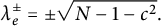 $$\begin{align*}\lambda_{e}^{\pm}=\pm \sqrt{N-1-c^2}.\end{align*}$$

Figure 2: Equilibria bifurcation diagram of system (3.4).
Thus, if
 $c=0$
, the only equilibrium is the equatorial one, which is a saddle. If
$c=0$
, the only equilibrium is the equatorial one, which is a saddle. If
 $0<|c|<\sqrt {N-1}$
, then the equatorial equilibrium is a saddle and the nonequatorial equilibria are centers. If
$0<|c|<\sqrt {N-1}$
, then the equatorial equilibrium is a saddle and the nonequatorial equilibria are centers. If
 $|c|\geq \sqrt {N-1}$
, then the only equilibrium is the equatorial one and it is a center. Note that the values
$|c|\geq \sqrt {N-1}$
, then the only equilibrium is the equatorial one and it is a center. Note that the values
 $c=\pm \sqrt {N-1}$
correspond to Hamiltonian pitchfork bifurcation values (see Figure 3).
$c=\pm \sqrt {N-1}$
correspond to Hamiltonian pitchfork bifurcation values (see Figure 3).

Figure 3: Phase portrait associated with the reduced Hamiltonian system (3.4).
Remark 3.1 Note that the nonequatorial relative equilibria are centers in the 1-d.o.f. reduced system, which implies that they are orbitally stable within homothetic ring solutions. On the other hand, in [Reference Hernández-Garduño, Pérez-Chavela and Zhu8], the authors prove for the cotangent potential that the orbital stability in the reduced manifold is guaranteed only for
 $\theta $
in a neighborhood of
$\theta $
in a neighborhood of
 $\pi /2$
,
$\pi /2$
,
 $\theta \neq \pi /2$
, and N odd.
$\theta \neq \pi /2$
, and N odd.
3.4 Nonlinear stability of the ring solution for
$\nu>0$
and
$\theta _0\in (0,\pi /2)$


It is clear that the nonlinear stability in the 1-d.o.f. system does not guarantee the nonlinear stability in the full system (1.6), but the instability in the reduced one is, in fact, a sufficient condition to assure instability in the full system.
In this section, we make a study of the nonlinear stability of the ring solution described in case (3.7).
The linearization matrix associated with the Hamiltonian system (3.6) along the equilibrium solution defined in (3.7) is given by
 $$\begin{align*}A=J Hess(\mathcal{H}(X_0))=\left( \begin{array}{cccc} 0 & 0 & 1 & 0 \\ -2\sqrt{N-1}\cot\theta_0\csc\theta_0 & 0 & 0 & \csc^2\theta_0 \\ -2(N-1)\cot^2\theta_0 & 0 & 0 & 2\sqrt{N-1}\cot\theta_0\csc\theta_0 \\ 0 & 0 & 0 & 0 \\ \end{array} \right),\end{align*}$$
whose eigenvalues are obtained as
 $$ \begin{align} \lambda_{1,2}=0,\quad \lambda_{3,4}=\pm i\sqrt{2(N-1)}\cot\theta_0, \end{align} $$
with
 $N\geq 2$
and
$N\geq 2$
and
 $\theta _0\in (0,\pi /2)$
is the colatitude angle of the ring. Although this solution is stable for the reduced system (3.4), we can not ensure that the full system will inherit this property (3.6).
$\theta _0\in (0,\pi /2)$
is the colatitude angle of the ring. Although this solution is stable for the reduced system (3.4), we can not ensure that the full system will inherit this property (3.6).
Let us denote by
 $a_2$
and
$a_2$
and
 $a_4$
the eigenvector and associated generalized eigenvector, respectively, associated with the null eigenvalue. Similarly, we denote by
$a_4$
the eigenvector and associated generalized eigenvector, respectively, associated with the null eigenvalue. Similarly, we denote by
 $a_1=r_1+is_1$
the eigenvector associated with the eigenvalue
$a_1=r_1+is_1$
the eigenvector associated with the eigenvalue
 $i\omega _1$
. A simple computation shows that
$i\omega _1$
. A simple computation shows that
 $a_2$
,
$a_2$
,
 $a_4$
,
$a_4$
,
 $r_1$
, and
$r_1$
, and
 $s_1$
are given by
$s_1$
are given by
 $$ \begin{align*} \begin{split} a_2=\left(\begin{array}{c}0\\1\\0\\0\end{array}\right), \,\, a_4=\left( \begin{array}{c} -\frac{\sin\theta_0\tan\theta_0}{\sqrt{N-1}}\\0\\0\\-\sin^2\theta_0\end{array}\right), \,\, r_1=\left(\begin{array}{c} 0\\ \frac{\sec\theta_0}{\sqrt{N-1}}\\ 1\\ 0\end{array}\right),\,\, s_1=\left(\begin{array}{c}-\frac{\tan\theta_0}{\sqrt{2(N-1)}}\\0\\0\\0\end{array}\right).\\ \end{split} \end{align*} $$
By using the algorithm provided in [Reference Markeev10], we construct the symplectic matrix
 $$\begin{align*}N=[\delta_1\kappa_ 1r_1\quad \delta_2\kappa_2a_2\quad \kappa_1s_1\quad \kappa_2a_4],\end{align*}$$
where
 $\delta _1=sgn(\lbrace r_1,s_1\rbrace )=1$
,
$\delta _1=sgn(\lbrace r_1,s_1\rbrace )=1$
,
 $\delta _2=sgn(\lbrace a_2,a_4\rbrace )=-1$
,
$\delta _2=sgn(\lbrace a_2,a_4\rbrace )=-1$
,
 $ \kappa _1 =\frac {1}{\sqrt {| \lbrace r_1,s_1\rbrace | }}$
, and
$ \kappa _1 =\frac {1}{\sqrt {| \lbrace r_1,s_1\rbrace | }}$
, and
 $ \kappa _2 =\frac {1}{\sqrt {|\lbrace a_2,a_4\rbrace |}}$
, where
$ \kappa _2 =\frac {1}{\sqrt {|\lbrace a_2,a_4\rbrace |}}$
, where
 $\{\, \cdot ,\cdot \}$
denotes the Poisson bracket between vectors, that is,
$\{\, \cdot ,\cdot \}$
denotes the Poisson bracket between vectors, that is,
 $\{u,v\}=u^TJv$
. By introducing the symplectic linear change of coordinates induced by the above matrix into the Hamiltonian (3.5), we obtain that the quadratic part assumes its normal form
$\{u,v\}=u^TJv$
. By introducing the symplectic linear change of coordinates induced by the above matrix into the Hamiltonian (3.5), we obtain that the quadratic part assumes its normal form
 $$ \begin{align} K_2=\frac{\omega_1}{2}(x^2+p_x^2)-\frac{p_y^2}{2}, \quad \omega_1=\sqrt{2(N-1)}\cot(\theta_0), \end{align} $$
with its corresponding transpose quadratic term
 $$ \begin{align} K^T_2=\frac{y^2}{2}-\frac{\omega_1}{2}(x^2+p_x^2). \end{align} $$
Remark 3.1 For the case where
 $\nu>0$
and
$\nu>0$
and
 $\theta \in (\pi /2,\pi )$
, the same steps of the previous case are followed and we obtain that
$\theta \in (\pi /2,\pi )$
, the same steps of the previous case are followed and we obtain that
 $$\begin{align*}K_2 = -\frac{\omega_1}{2}(x^2+p_x^2)-\frac{p_y^2}{2} \mbox{ and } K^T_2=\frac{y^2}{2}+\frac{\omega_1}{2}(x^2+p_x^2).\end{align*}$$
We are now assuming that the Hamiltonian (3.5) is written in the coordinates that normalize the quadratic terms of the Taylor expansion. We proceed to normalize the cubic terms by introducing a near identity symplectic coordinates obtained through a suitable generating function (see Appendix B) and taking into account the Lie equation
 $\{G_3, K_2^T\}=0$
, we get that the normalized third-order terms are given by
$\{G_3, K_2^T\}=0$
, we get that the normalized third-order terms are given by
 $$ \begin{align} G_3=y(x^2+p_x^2)g_{2100}+y^3 g_{0300}, \end{align} $$
with coefficients
 $$ \begin{align*} \begin{split} g_{0300} & = -\frac{\sqrt[4]{8(N-1)} (4+\cos(2\theta_0))\csc^4\theta_0\sec\theta_0}{3\sqrt{\tan\theta_0}},\\ g_{2100} & =-\frac{\sec^3\theta_0+\sqrt{2(N-1)^5}(4+\cos(2\theta_0))\csc^3(\theta_0)}{\sqrt[4]{8(N-1)^5}\tan ^{\frac{3}{2}}\theta_0} \end{split} \end{align*} $$
(see Appendix B.1 for the explicit coefficients of the generating function).
Therefore, we have that
 $g_{0300}\neq 0$
, for all
$g_{0300}\neq 0$
, for all
 $\theta _0\in (0,\pi /2)$
and, according to Sokol’skii’s Theorem (A.1), we conclude that the equilibrium is unstable in the Lyapunov sense.
$\theta _0\in (0,\pi /2)$
and, according to Sokol’skii’s Theorem (A.1), we conclude that the equilibrium is unstable in the Lyapunov sense.
Remark 3.2 In the case where
 $\nu>0$
and
$\nu>0$
and
 $\theta _0\in (\pi /2,\pi )$
, we have that the terms of degree three in their normal form is as in (3.15), where
$\theta _0\in (\pi /2,\pi )$
, we have that the terms of degree three in their normal form is as in (3.15), where
 $g_{0300}$
is given by
$g_{0300}$
is given by
 $$\begin{align*}g_{0300}=\frac{\sqrt[4]{8(N-1)} (4+\cos(2\theta_0))\csc^4\theta_0\sec\theta_0}{3\sqrt{|\tan\theta_0|}}\neq0.\end{align*}$$
Proposition 3.1 The ring solution is Lyapunov unstable for any
 $\nu $
and
$\nu $
and
 $\theta _0\in (0,\pi )\setminus \{ \pi /2 \}$
.
$\theta _0\in (0,\pi )\setminus \{ \pi /2 \}$
.
4 Periodic orbits
In this section, we will study some periodic solutions of the N-body problem on the sphere
 $\mathbb {S}^2$
emerging from the ring solution. More precisely, we look for periodic solutions that preserve the regular polygon configuration of the bodies, but not necessarily rotating uniformly in a fixed parallel. For this purpose, we first note that in the reduced 1-d.o.f. system, the nonequatorial equilibrium point
$\mathbb {S}^2$
emerging from the ring solution. More precisely, we look for periodic solutions that preserve the regular polygon configuration of the bodies, but not necessarily rotating uniformly in a fixed parallel. For this purpose, we first note that in the reduced 1-d.o.f. system, the nonequatorial equilibrium point
 $(\theta _0,0)$
given in (3.11) is surrounded by periodic orbits whenever
$(\theta _0,0)$
given in (3.11) is surrounded by periodic orbits whenever
 $c\in (0,\sqrt {N-1})$
. Let
$c\in (0,\sqrt {N-1})$
. Let
 $\eta (t)=(\theta (t), p_{\theta }(t))$
one of these periodic solutions with
$\eta (t)=(\theta (t), p_{\theta }(t))$
one of these periodic solutions with
 $\eta (0)=(\theta ,0)$
and period
$\eta (0)=(\theta ,0)$
and period
 $\tau (\theta )$
, then we need to find a suitable initial value
$\tau (\theta )$
, then we need to find a suitable initial value
 $\theta (0)=\theta \in (\pi /2,\theta _0)$
such that the variable
$\theta (0)=\theta \in (\pi /2,\theta _0)$
such that the variable
 $\varphi $
in (3.2) verifies the equation
$\varphi $
in (3.2) verifies the equation
 $$ \begin{align} \varphi(n \tau(\theta))=\varphi(0)\mod(2\pi), \end{align} $$
for some
 $n\in \mathbb {N}$
. By using the integral form of
$n\in \mathbb {N}$
. By using the integral form of
 $\varphi (t)$
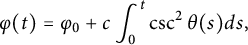 $$ \begin{align} \varphi(t) = \varphi_0 + c \int_0^t \csc^2\theta(s)ds, \end{align} $$
and taking into account that
 $\theta (s)$
is a
$\theta (s)$
is a
 $\tau (\theta )$
-periodic function, we get that equation (4.1) assumes the form
$\tau (\theta )$
-periodic function, we get that equation (4.1) assumes the form
 $$ \begin{align} \frac{c}{2\pi}\int_0^{\tau(\theta)} \csc^2\theta(s,\theta)ds = \frac{m}{n}. \end{align} $$
Now, we define
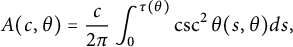 $$ \begin{align} A(c,\theta)=\frac{c}{2\pi}\int_0^{\tau(\theta)} \csc^2\theta(s,\theta)ds, \end{align} $$
and note that if we fix c in (4.4), we can take
 $A(c,\theta )$
as a function depending only on
$A(c,\theta )$
as a function depending only on
 $ \theta $
, namely,
$ \theta $
, namely,
 $f(\theta )$
. Next, we define the function
$f(\theta )$
. Next, we define the function
 $g(x,\theta )=f(\theta )-x$
. If
$g(x,\theta )=f(\theta )-x$
. If
 $\theta =\theta _0$
is a nonequatorial equilibrium and denoting by
$\theta =\theta _0$
is a nonequatorial equilibrium and denoting by
 $\tau _0=\tau (\theta _0)$
, with
$\tau _0=\tau (\theta _0)$
, with
 $\tau _0$
a value that will be suitable chosen later, then it follows that
$\tau _0$
a value that will be suitable chosen later, then it follows that
 $$ \begin{align} g(x,\theta_0) = \frac{\nu\tau_0}{2\pi}-x\,\, \mbox{ and }\,\, \varphi(t)= \varphi_0 + \nu t, \end{align} $$
with
 $\nu =c \csc ^2\theta _0$
. Since
$\nu =c \csc ^2\theta _0$
. Since
 $\varphi $
is
$\varphi $
is
 $\frac {2\pi }{\nu }$
-periodic, we can choose
$\frac {2\pi }{\nu }$
-periodic, we can choose
 $\tau _0=\frac {2\pi }{\nu }$
and obtain that
$\tau _0=\frac {2\pi }{\nu }$
and obtain that
 $g(x,\theta _0)=1-x$
. Now, we can easily see that
$g(x,\theta _0)=1-x$
. Now, we can easily see that
 $$\begin{align*}g(1,\theta_0)=0\quad \text{y}\quad \left.\frac{\partial g(x,\theta)}{\partial x}\right|{}_{(1,\theta_0)}=-1\neq 0.\end{align*}$$
Then, by the Implicit Function Theorem, we have that there are open intervals
 $I_{\varepsilon } =\left (\theta _0-\varepsilon ,\theta _0+\varepsilon \right )$
and
$I_{\varepsilon } =\left (\theta _0-\varepsilon ,\theta _0+\varepsilon \right )$
and
 $J=(1 -\delta , 1 + \delta )$
such that
$J=(1 -\delta , 1 + \delta )$
such that
 $g(x,\theta )=0$
, for all
$g(x,\theta )=0$
, for all
 $(x,\theta )\in J\times I_{\varepsilon }$
. Furthermore, there exists a
$(x,\theta )\in J\times I_{\varepsilon }$
. Furthermore, there exists a
 $C^k$
class function,
$C^k$
class function,
 $x : I_{\varepsilon } \rightarrow J$
, such that
$x : I_{\varepsilon } \rightarrow J$
, such that
 $g(x(\theta ),\theta )=0$
and
$g(x(\theta ),\theta )=0$
and
 $x(\theta _0)=1$
. Then, by density of
$x(\theta _0)=1$
. Then, by density of
 $\mathbb {Q}$
en
$\mathbb {Q}$
en
 $\mathbb {R}$
, we have that
$\mathbb {R}$
, we have that
 $J\cap \mathbb {Q}\neq \emptyset $
. Therefore, the set
$J\cap \mathbb {Q}\neq \emptyset $
. Therefore, the set
 $\Upsilon =x^{-1}(J\cap \mathbb {Q})\neq \emptyset $
, is such that given
$\Upsilon =x^{-1}(J\cap \mathbb {Q})\neq \emptyset $
, is such that given
 $m/n\in J\cap \mathbb {Q}$
, there exists
$m/n\in J\cap \mathbb {Q}$
, there exists
 $\theta ^*\in \Upsilon $
such that
$\theta ^*\in \Upsilon $
such that
 $g(m/n,\theta ^*)=0$
. Therefore, we conclude that there are initial conditions
$g(m/n,\theta ^*)=0$
. Therefore, we conclude that there are initial conditions
 $\theta ^*$
that generate periodic orbits in the complete system.
$\theta ^*$
that generate periodic orbits in the complete system.
4.1 Some examples of periodic orbits on the sphere
$\mathbb {S}^2$

In this section, we present some examples of periodic orbits on the sphere
 $\mathbb {S}^2$
obtained through the method described above. Note that the initial conditions that generate polygonal periodic orbits are the zeros of the equation (4.3). Thus, for a fixed value of c, we can consider the graph of the function
$\mathbb {S}^2$
obtained through the method described above. Note that the initial conditions that generate polygonal periodic orbits are the zeros of the equation (4.3). Thus, for a fixed value of c, we can consider the graph of the function
 $f(\theta )=A(c,\theta )$
and approximate their intersections with horizontal lines of the form
$f(\theta )=A(c,\theta )$
and approximate their intersections with horizontal lines of the form
 $y=m/n$
.
$y=m/n$
.
For the case
 $N=2$
, the value of c must be chosen such that
$N=2$
, the value of c must be chosen such that
 $|c|<1$
. In particular, for
$|c|<1$
. In particular, for
 $c=(2+\sqrt {3})/5$
the graph of
$c=(2+\sqrt {3})/5$
the graph of
 $A(c,\theta )$
is shown in Figure 4.
$A(c,\theta )$
is shown in Figure 4.

Figure 4: Graph of the function
 $f(\theta )=A(c,\theta )$
for
$f(\theta )=A(c,\theta )$
for
 $N=2$
and
$N=2$
and
 $ c=(2+\sqrt {3})/5$
.
$ c=(2+\sqrt {3})/5$
.
The following table gives initial conditions for some values of
 $(m,n)$
and their corresponding period.
$(m,n)$
and their corresponding period.
In Table 1, for different rationals
 $m/n$
, we find initial conditions
$m/n$
, we find initial conditions
 $\theta ^*$
giving rise to periodic orbits in the complete system. Some of them are located close to the equilibrium
$\theta ^*$
giving rise to periodic orbits in the complete system. Some of them are located close to the equilibrium
 $\theta _0=2.298941328617731`$
and others are close to the homoclinic orbit shown in Figure 3b, which also correspond to periodic orbits that cross the equator. Similarly, near the symmetric equilibrium
$\theta _0=2.298941328617731`$
and others are close to the homoclinic orbit shown in Figure 3b, which also correspond to periodic orbits that cross the equator. Similarly, near the symmetric equilibrium
 $\theta _0=0.8426513249720621`$
, we can also find initial conditions that give periodic solutions in the whole system (Figure 5).
$\theta _0=0.8426513249720621`$
, we can also find initial conditions that give periodic solutions in the whole system (Figure 5).

Figure 5: Periodic orbits on the sphere
 $\mathbb {S}^2$
for
$\mathbb {S}^2$
for
 $N=2$
,
$N=2$
,
 $c=(2+\sqrt {3})/5$
with initial condition given in Table 1.
$c=(2+\sqrt {3})/5$
with initial condition given in Table 1.
Table 1: Initial conditions
 $\theta ^*$
and periods
$\theta ^*$
and periods
 $T_F$
that give rise to periodic orbits in the complete system for
$T_F$
that give rise to periodic orbits in the complete system for
 $N=2$
and
$N=2$
and
 $ c=(2+\sqrt {3})/5$
.
$ c=(2+\sqrt {3})/5$
.

For the case
 $N=3$
, the value of c must be chosen such that
$N=3$
, the value of c must be chosen such that
 $|c|<\sqrt {2}$
. In particular, for
$|c|<\sqrt {2}$
. In particular, for
 $c=1-\sqrt {3}/5$
the graph of
$c=1-\sqrt {3}/5$
the graph of
 $A(c,\theta )$
is shown in Figure 6.
$A(c,\theta )$
is shown in Figure 6.

Figure 6: Graph of the function
 $f(\theta )=A(c,\theta )$
for
$f(\theta )=A(c,\theta )$
for
 $N=3$
and
$N=3$
and
 $ c=1-\sqrt {3}/5$
.
$ c=1-\sqrt {3}/5$
.
The following table gives initial conditions for some values of
 $(m,n)$
and their corresponding period.
$(m,n)$
and their corresponding period.
In Table 2, for different rationals
 $m/n$
, we can find initial conditions
$m/n$
, we can find initial conditions
 $\theta ^*$
that give rise to periodic orbits in the complete system. Some of them are close to the equilibrium
$\theta ^*$
that give rise to periodic orbits in the complete system. Some of them are close to the equilibrium
 $\theta _0=2.6611657363097923`$
(or in the symmetric equilibrium
$\theta _0=2.6611657363097923`$
(or in the symmetric equilibrium
 $\theta _0=0.48042691728000075`$
), and others are close to the homoclinic orbit shown in Figure 3b. Moreover, we chose all initial conditions except row 5 inside the homoclinic orbit (Figure 7).
$\theta _0=0.48042691728000075`$
), and others are close to the homoclinic orbit shown in Figure 3b. Moreover, we chose all initial conditions except row 5 inside the homoclinic orbit (Figure 7).

Figure 7: Periodic orbits on the sphere
 $\mathbb {S}^2$
for
$\mathbb {S}^2$
for
 $N=3$
,
$N=3$
,
 $c=1-\sqrt {3}/5$
with initial condition given in Table 2.
$c=1-\sqrt {3}/5$
with initial condition given in Table 2.
Table 2: Initial conditions
 $\theta ^*$
and periods
$\theta ^*$
and periods
 $T_F$
that give rise to periodic orbits in the complete system for
$T_F$
that give rise to periodic orbits in the complete system for
 $N=3$
and
$N=3$
and
 $ c=1-\sqrt {3}/5$
.
$ c=1-\sqrt {3}/5$
.

For the case
 $N=4$
, the value of c must be chosen such that
$N=4$
, the value of c must be chosen such that
 $|c|<\sqrt {3}$
. In particular, for
$|c|<\sqrt {3}$
. In particular, for
 $c=2\sqrt {5+\sqrt {2}}/5$
the graph of
$c=2\sqrt {5+\sqrt {2}}/5$
the graph of
 $A(c,\theta )$
is shown in Figure 8.
$A(c,\theta )$
is shown in Figure 8.

Figure 8: Graph of the function
 $f(\theta )=A(c,\theta )$
for
$f(\theta )=A(c,\theta )$
for
 $N=4$
and
$N=4$
and
 $ c=2\sqrt {5+\sqrt {2}}/5$
.
$ c=2\sqrt {5+\sqrt {2}}/5$
.
The following table gives initial conditions for some values of
 $(m,n)$
and their corresponding period.
$(m,n)$
and their corresponding period.
In Table 3, we find initial conditions
 $\theta ^*$
leading to periodic orbits in the complete system for different rationals
$\theta ^*$
leading to periodic orbits in the complete system for different rationals
 $m/n$
. Some of them are close to the equilibrium
$m/n$
. Some of them are close to the equilibrium
 $\theta _0=2.51685340624551`$
(or in the symmetric equilibrium
$\theta _0=2.51685340624551`$
(or in the symmetric equilibrium
 $\theta _0=0.6247392473442833`$
), and others are close to the homoclinic orbit shown in Figure 3b. Moreover, we chose all initial conditions except row 5 inside the homoclinic orbit (Figure 9).
$\theta _0=0.6247392473442833`$
), and others are close to the homoclinic orbit shown in Figure 3b. Moreover, we chose all initial conditions except row 5 inside the homoclinic orbit (Figure 9).

Figure 9: Periodic orbits on the sphere
 $\mathbb {S}^2$
for
$\mathbb {S}^2$
for
 $N=4$
,
$N=4$
,
 $c=2\sqrt {5+\sqrt {2}}/5$
with initial condition given in Table 3.
$c=2\sqrt {5+\sqrt {2}}/5$
with initial condition given in Table 3.
Table 3: Initial conditions
 $\theta ^*$
and periods
$\theta ^*$
and periods
 $T_F$
that give rise to periodic orbits in the complete system for
$T_F$
that give rise to periodic orbits in the complete system for
 $N=4$
and
$N=4$
and
 $ c=2\sqrt {5+\sqrt {2}}/5$
.
$ c=2\sqrt {5+\sqrt {2}}/5$
.

A Reduced system
A.1 Reduction to two degrees of freedom
In this section, we will see the details regarding the reduction of the system (1.6) to a Hamiltonian system with two degrees of freedom. For this, let us consider the Hamiltonian function defined in (1.7), then we see that from the first equation of the system (1.6) the moment
 $p_{\varphi _j}$
is given by
$p_{\varphi _j}$
is given by
 $$ \begin{align} p_{\varphi_j}=\dot{\varphi}_j\sin^2\theta_j. \end{align} $$
Differentiating with respect to time in this last relation and using the third equation defined in (1.6), we find the following equality:
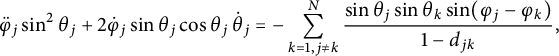 $$ \begin{align} \ddot{\varphi}_j\sin^2\theta_j+2\dot{\varphi}_j\sin\theta_j\cos\theta_j\,\dot{\theta}_j=-\sum_{k=1,j\neq k}^{N}\frac{\sin\theta_j\sin\theta_k\sin(\varphi_j-\varphi_k)}{1-d_{jk}}, \end{align} $$
and having into account that
 $$\begin{align*}\sum_{k=1,j\neq k}^{N}\frac{\sin\theta_j\sin\theta_k\sin(\varphi_j-\varphi_k)}{1-d_{jk}}=-\sum_{k=1,j\neq k}^{N}\frac{\sin\theta_k\sin\theta_j\sin(\varphi_k-\varphi_j)}{1-d_{kj}},\end{align*}$$
we finally get
 $$\begin{align*}\sum_{j=1}^N\sum_{k=1,j\neq k}^{N}\frac{\sin\theta_j\sin\theta_k\sin(\varphi_j-\varphi_k)}{1-d_{jk}}=0.\end{align*}$$
Therefore, using this last relation together with (3.1) in (A.2), we have
 $$ \begin{align*} \begin{split} 0&=\sum_{j=1}^N\ddot{\varphi}_j\sin^2\theta_j+2\dot{\varphi}_j\sin\theta_j\cos\theta_j\,\dot{\theta}_j\\ &=\sum_{j=1}^N\ddot{\varphi}\sin^2\theta+2\dot{\varphi}\sin\theta\cos\theta\,\dot{\theta}\\ &=N(\ddot{\varphi}\sin^2\theta+2\dot{\varphi}\sin\theta\cos\theta\,\dot{\theta})\\ &=\ddot{\varphi}\sin^2\theta+2\dot{\varphi}\sin\theta\cos\theta\,\dot{\theta}\\ &=\frac{d}{dt}(\dot{\varphi}\sin^2\theta)=\dot{p}_{\varphi}.\\ \end{split} \end{align*} $$
On the other hand, differentiating the second equation obtained in (1.6) and using the fourth equation of the system (1.6) together with (A.2), we obtain
 $$ \begin{align*} \begin{split} \ddot{\theta}_j&=\cot\theta_j\csc^2\theta_jp_{\varphi_j}^2-\sum_{k=1,j\neq k}^{N}\frac{\cos\theta_k\sin\theta_j-\cos\theta_j\sin\theta_k\cos(\varphi_j-\varphi_k)}{1-d_{jk}}\\ &=\cot\theta_j\csc^2\theta_j(\dot{\varphi}_j\sin^2\theta_j)^2-\sum_{k=1,j\neq k}^{N}\frac{\cos\theta_k\sin\theta_j-\cos\theta_j\sin\theta_k\cos(\varphi_j-\varphi_k)}{1-d_{jk}}\\ &=\cos\theta_j\sin\theta_j\,\dot{\varphi}_j^2-\sum_{k=1,j\neq k}^{N}\frac{\cos\theta_k\sin\theta_j-\cos\theta_j\sin\theta_k\cos(\varphi_j-\varphi_k)}{1-d_{jk}}.\\ \end{split} \end{align*} $$
Again, in this last relation, we can use the equations defined in (3.1) to get
 $$ \begin{align*} \begin{split} \ddot{\theta}&=\cos\theta\sin\theta\,\dot{\varphi}^2-\cos\theta\sin\theta\sum_{k=1,j\neq k}^{N}\frac{1-\cos(\varphi_j-\varphi_k)}{1-\cos^2\theta-\sin^2\theta\cos(\varphi_j-\varphi_k)}\\ &=\cos\theta\sin\theta\,\dot{\varphi}^2-(N-1)\cot\theta.\\ &=\frac{\cos\theta}{\sin^3\theta}(\sin^2\theta\,\dot{\varphi})^2-(N-1)\cot\theta.\\ &=\cot\theta\csc^2\theta\,p_{\varphi}^2-(N-1)\cot\theta.\\ \end{split} \end{align*} $$
Therefore, we obtain that our reduced Hamiltonian is a Hamiltonian with two degrees of freedom of the form
 $$\begin{align*}\mathcal{H}=\frac{1}{2}(\csc^2\theta p_{\varphi}^2+p_{\theta}^2)+(N-1)\ln(\sin\theta).\end{align*}$$
A.2 Sokol’skii stability theorem 1977
Suppose that the Hamiltonian function in its normal form admits the following form:
 $$ \begin{align} H=\frac{\delta_1}{2}q_1^2+\frac{\omega\delta_2}{2}(q_2^2+p_2^2)+\sum_{s=3}^{M}\sum_{j=0}^{[s/2]}a_{s-2j,j}\,p_1^{s-2j}(q_2^2+p_2^2)^j+H^{M+1}+\cdots, \end{align} $$
where
 $a_{s-2j,j}$
are real constants. The normalization must be carried out up to terms of order M such that
$a_{s-2j,j}$
are real constants. The normalization must be carried out up to terms of order M such that
 $a_{M,0}$
is different from zero.
$a_{M,0}$
is different from zero.
Theorem A.1 (A.G. Sokol’skii, 1977)
Suppose that a canonic system with two degrees of freedom has one zero frequency and multiple elementary divisors and that its Hamiltonian function has been reduced to form (A.3). Then:
-
(1) If M is odd, the equilibrium position is unstable.
-
(2) If M is even and
$\delta _1a_{M,0}<0$
, the equilibrium position is unstable. -
(3) If M is even and
$\delta _1a_{M,0}>0$
, the equilibrium position is Lyapunov-stable.


For more information, see [Reference Sokol’skii12].
B Normal form of high-order terms
Let us consider the Taylor expansion of H
 $$\begin{align*}H=H_2+H_3+H_4+\cdots+H_s+\cdots,\end{align*}$$
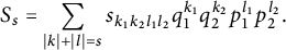
with
 $$\begin{align*}H_s=\sum_{|k|+|l|=s}h_{k_1k_2l_1l_2}q_1^{k_1}q_2^{k_2}p_1^{l_1}p_2^{l_2},\end{align*}$$
and
 $H_2$
in its normal form. The normalized Hamiltonian G of H is obtained via the Lie algorithm
$H_2$
in its normal form. The normalized Hamiltonian G of H is obtained via the Lie algorithm
 $$\begin{align*}G=G_2+G_3+G_4+\cdots+G_s+\cdots,\end{align*}$$
where
 $G_2=H_2$
and
$G_2=H_2$
and
 $G_s$
are homogeneous polynomials of degree s
$G_s$
are homogeneous polynomials of degree s
 $$\begin{align*}G_s=\sum_{|k|+|l|=s}g_{k_1k_2l_1l_2}q_1^{k_1}q_2^{k_2}p_1^{l_1}p_2^{l_2}.\end{align*}$$
Similarly, we define the generating function of the symplectic transformation that becomes H into G, denoted by
 $$ \begin{align} W=q_1p_1+q_2p_2+S_3+S_4+\cdots+S_s+\cdots, \end{align} $$
where
 $S_s$
are homogeneous polynomials of degree s, so that
$S_s$
are homogeneous polynomials of degree s, so that
 $$\begin{align*}S_s=\sum_{|k|+|l|=s}s_{k_1k_2l_1l_2}q_1^{k_1}q_2^{k_2}p_1^{l_1}p_2^{l_2}.\end{align*}$$
B.1 Normal form of the third-order terms with quadratic part as (3.13)
Since, in our case, the quadratic term is degenerated, the Lie equation takes the form
 $\{H^T_0,G_s\}=0$
. We start with the case
$\{H^T_0,G_s\}=0$
. We start with the case
 $s=3$
; that is, we will determine the Lie normal form of the terms
$s=3$
; that is, we will determine the Lie normal form of the terms
 $H_3$
of degree three of the Hamiltonian H under the assumption that the quadratic part
$H_3$
of degree three of the Hamiltonian H under the assumption that the quadratic part
 $H_2$
is already normalized. Furthermore, the matrix associated with the linear system is nondiagonalizable. Therefore, we must solve the system of equations generated by the following Lie equation:
$H_2$
is already normalized. Furthermore, the matrix associated with the linear system is nondiagonalizable. Therefore, we must solve the system of equations generated by the following Lie equation:
 $$\begin{align*}\{K^T_2,G_3\}=0,\end{align*}$$
where
 $K_2^T$
is defined in equation (3.14). From where we get that
$K_2^T$
is defined in equation (3.14). From where we get that
 $$ \begin{align*} \begin{split} &g_{3000}= 0,\,g_{2010}= 0,\,g_{2001}= 0,\,g_{1200}= 0,\,g_{1110}= 0,\,g_{1101}= 0,\,g_{1020}= 0,\\ &g_{1011}= 0,\,g_{1002}= 0,\,g_{0210}= 0,\,g_{0201}= 0,\,g_{0111}= 0,\,g_{0102}= 0,\,g_{0030}= 0,\\ &g_{0021}= 0,\,g_{0012}= 0,\,g_{0003}= 0,\,g_{0120}= g_{2100}. \end{split} \end{align*} $$
Therefore, the terms of degree three of the normalized Hamiltonian are given by
 $$ \begin{align} G_3=y(x^2+p_x^2)g_{2100}+y^3 g_{0300}. \end{align} $$
Furthermore, according to the Lie triangle and the recurrence formula, we have
 $$ \begin{align} G_3=H_3+\{H^T_0,S_3\}\equiv H_2+G_3\left|{}_{\left(q_1,q_2,\frac{\partial W}{\partial q_1},\frac{\partial W}{\partial q_2}\right)} \right.=H_2+H_3\left|{}_{\left(\frac{\partial W}{\partial p_1},\frac{\partial W}{\partial p_2},p_1,p_2\right)} \right.. \end{align} $$
It is verified that equation (B.3) is satisfied for
 $G_3$
is as it appears in (B.2), for this purpose, we must choose the coefficients of
$G_3$
is as it appears in (B.2), for this purpose, we must choose the coefficients of
 $S_3$
in a convenient way. More precisely,
$S_3$
in a convenient way. More precisely,
 $$ \begin{align*} \begin{split} s_{3000}&= \frac{3\sqrt[4]{2}\tan\theta_0\sec^2\theta_0+2^{7/4}(N-1)^{5/2}(4+\cos(2\theta_0))\csc^2\theta_0}{9(N-1)^{3/4} \omega_1\tan^{\frac{5}{2}}\theta_0},\\ s_{2100}&= -\frac{(2+\cos(2\theta_0))\csc^3\theta_0\sec\theta_0((N-1)\omega_1\cos(2\theta_0)+(N-1)\omega_1-2)}{2\sqrt{2}\omega_1},\\ s_{2010}&=0,\quad s_{2001}=0,\quad s_{0102}= 0,\quad s_{0003}=0,\\ s_{1200}&= \frac{\sqrt[4]{8(N-1)^3} (4+\cos(2\theta_0))\csc^4\theta_0}{\omega_1\sqrt{\tan\theta_0}},\\ s_{1110}&= \frac{\sqrt{2(N-1)^5}(4+\cos(2\theta_0))\csc^3\theta_0-\sec^3\theta_0}{\sqrt[4]{8(N-1)^5}\omega_1\tan ^{\frac{3}{2}}\theta_0},\\ s_{1101}&= -\frac{2\sqrt{2}\csc\theta_0(2(N-1)\omega_1+3(1-(N-1)\omega_1)\csc^2\theta_0+\sec^2\theta_0)}{\sqrt{N-1} \omega_1^2},\\ s_{1020}&= \frac{2^{3/4} (N-1)^{7/4} (4+ \cos (2 \theta_0)) \csc ^2\theta_0}{3 \omega_1 \tan ^{\frac{5}{2}}\theta_0},\\ s_{1011}&= \frac{(2+\cos (2 \theta_0)) \csc ^3\theta_0 \sec \theta_0 ((N-1) \omega_1 \cos (2 \theta_0)+(N-1) \omega_1-2)}{2\sqrt{2} \omega_1^2},\\ s_{1002}&= -\frac{\sqrt[4]{2} \left(2\omega_1\sec^2\theta_0-(N-1)\omega_1^2+2 \sqrt{2} (N-1)^{3/2} (4+\cos (2 \theta_0)) \csc ^3\theta_0 \sec \theta_0\right)}{(N-1)^{3/4} \omega_1^3 \tan ^{\frac{3}{2}}\theta_0},\\ s_{0300}&= -\frac{\sqrt{2}}{3}\csc\theta_0(3\cot\theta_0\csc\theta_0+\sec \theta_0),\\ s_{0210}&= -\frac{\sqrt{2}\csc\theta_0(3\csc^2\theta_0 +\sec^2\theta_0)}{\sqrt{N-1} \omega_1},\\ s_{0201}&= -\frac{\csc \theta_0}{\sqrt[4]{8(N-1)} \sqrt{\tan \theta_0}}, \end{split} \end{align*} $$
 $$ \begin{align*} \begin{split} s_{0120}&= -\frac{(2+\cos (2 \theta_0)) \csc ^3\theta_0 \sec \theta_0 ((N-1) \omega_1 \cos (2 \theta_0)+(N-1) \omega_1+2)}{2\sqrt{2} \omega_1},\\ s_{0111}&= -\frac{2 \sqrt[4]{2} \csc ^4\theta_0\left(\omega_1 \sin ^3\theta_0\sec\theta_0+\sqrt{2} (N-1)^{3/2}(4+\cos(2\theta_0))\right)}{(N-1)^{3/4} \omega_1^2 \sqrt{\tan\theta_0}},\\ s_{0030}&= -\frac{\sqrt{2(N-1)} (2+\cos (2 \theta_0)) \csc ^3\theta_0}{3 \omega_1},\\ s_{0021}&=-\frac{\sqrt{2(N-1)^5}(4+\cos (2 \theta_0))+4(N-1)\omega_1\sec\theta_0- \sec ^3\theta_0}{2\sqrt{2(N-1)^5}\omega_1^2 \tan ^{\frac{3}{2}}\theta_0},\\ s_{0012}&= \frac{2\sqrt{2}\csc\theta_0(2(N-1)\omega_1+3(1-(N-1)\omega_1)\csc^2\theta_0+\sec^2\theta_0)}{\sqrt{N-1} \omega_1^3}. \end{split} \end{align*} $$
This choice of the coefficients of the generating function implies that the terms of degree three of the normalized Hamiltonian are given by (B.2), where
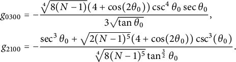 $$ \begin{align*} \begin{split} g_{0300} & = -\frac{\sqrt[4]{8(N-1)} (4+\cos(2\theta_0))\csc^4\theta_0\sec\theta_0}{3\sqrt{\tan\theta_0}},\\ g_{2100} & =-\frac{\sec^3\theta_0+\sqrt{2(N-1)^5}(4+\cos(2\theta_0))\csc^3(\theta_0)}{\sqrt[4]{8(N-1)^5}\tan ^{\frac{3}{2}}\theta_0}. \end{split} \end{align*} $$


