Antarctic regional modelling of atmospheric, sea-ice and oceanic processes and validation with observations

Abstract

High-latitude interactions of local-scale processes in the atmosphere-ice-ocean system have effects on the local, Antarctic and global climate. Phenomena including polynyas and leads are examples of such interactions which, when combined, have a significant impact on larger scales. These small-scale features, which are typically parameterized in global models, can be explicitly simulated using high-resolution regional climate system models. As such, the study of these interactions is well suited to a regional model approach and is considered here using the Arctic Regional Climate System Model (ARCSyM). This model has been used for many simulations in the Arctic, and is now implemented for the Antarctic. Observations of such processes in the Antarctic are limited, which makes model validation difficult. However, using the best available observations for an annual cycle, we have determined a suite of model parameterization which allows us to reasonably simulate the Antarctic climate. This work considers a fine-resolution (20 km) simulation in the Cosmonaut Sea region, with the eventual goal of elucidating the mechanisms in the formation and maintenance of the sensible-heat polynya which is a regular occurrence in this area. It was found in an atmosphere-sea-ice simulation that the ocean plays an important role in regulating the sea-ice cover in this region in compensating for the cold atmospheric conditions.

Introduction

The variability of sea-ice cover is of particular interest in studies of the effects of the Antarctic region on global climate. Simmonds and Budd (1991) found that the variable fractions of open water in the sea ice in global model simulations had a marked influence on the polar and global atmospheric circulation. Wu and others (1996b) showed that the instantaneous removal of the Antarctic sea-ice cover had a significant impact on the Southern Hemisphere climate. In addition, sea-ice processes are thought to contribute cold saline deep water to the global ocean thermohaline circulation through brine rejection during ice formation (Killworth, 1983).

One aspect of sea-ice variability is the occurrence of polynyas (large areas of open water or reduced ice concentration in the ice pack). Deep-ocean sensible-heat polynyas in particular are an important aspect of climate variability because of their relative size (up to 20% of the overall Antarctic sea-ice cover) and likely impact on ocean ventilation, Bottom Water formation and atmospheric circulation. For example, the exchange of heat and moisture between the atmosphere and ocean in the presence of the Weddell Sea polynya has been shown in global simulations to have a large effect on the variability of the Antarctic and global climate (Glowienka-Hense, 1995).

Deep-water or sensible-heat polynyas are thought to be initiated and maintained primarily by ice melt due to deep-ocean convection, as opposed to ice advection out of the area by atmospheric or oceanic forcing, as in the case of coastal or latent-heat polynyas. However, studies of these polynyas have not yet revealed the relative importance of ice melt and ice advection, nor identified the crucial mechanisms in polynya formation and maintenance. Hence, the true nature of such polynyas is not well understood.

Comiso and Gordon (1987) first noted the appearance of areas of reduced sea-ice concentration in the regions of Maud Rise and the Cosmonaut Sea (see Fig. 1), labelling them the Maud Rise and Cosmonaut polynyas, respectively. These features were discovered in 2 day averaged ice-concentration maps (1973–87) derived from the Nimbus 7 Scanning Multichannel Microwave Radiometer (SMMR). They also noted that both of these polynyas were of a more transient nature than the more persistent Weddell polynya. More recent (1987–93) satellite observations with the arrival of the Special Sensor Microwave/Imager (SSM/I) have indicated the continued recurrence of a deep-water polynya in the Cosmonaut Sea region (Comiso and Gordon, 1996). The Cosmonaut polynya is significant because of its large size (averaging 7.2 × 104^km2) and because it may provide a model for similar transient deep-water polynyas. The Cosmonaut polynya is thought to be initiated and maintained primarily by upwelling of warmer Circumpolar Deep Water causing ice melt and a divergence of surface water (Comiso and Gordon, 1996), as opposed to deep-ocean convection, the main mechanism in the formation of the Weddell polynya. During a voyage of the japanese Antarctic Research Expedition, the Cosmonaut polynya was found not to have the anomalously cold water typically associated with deep-ocean convection.

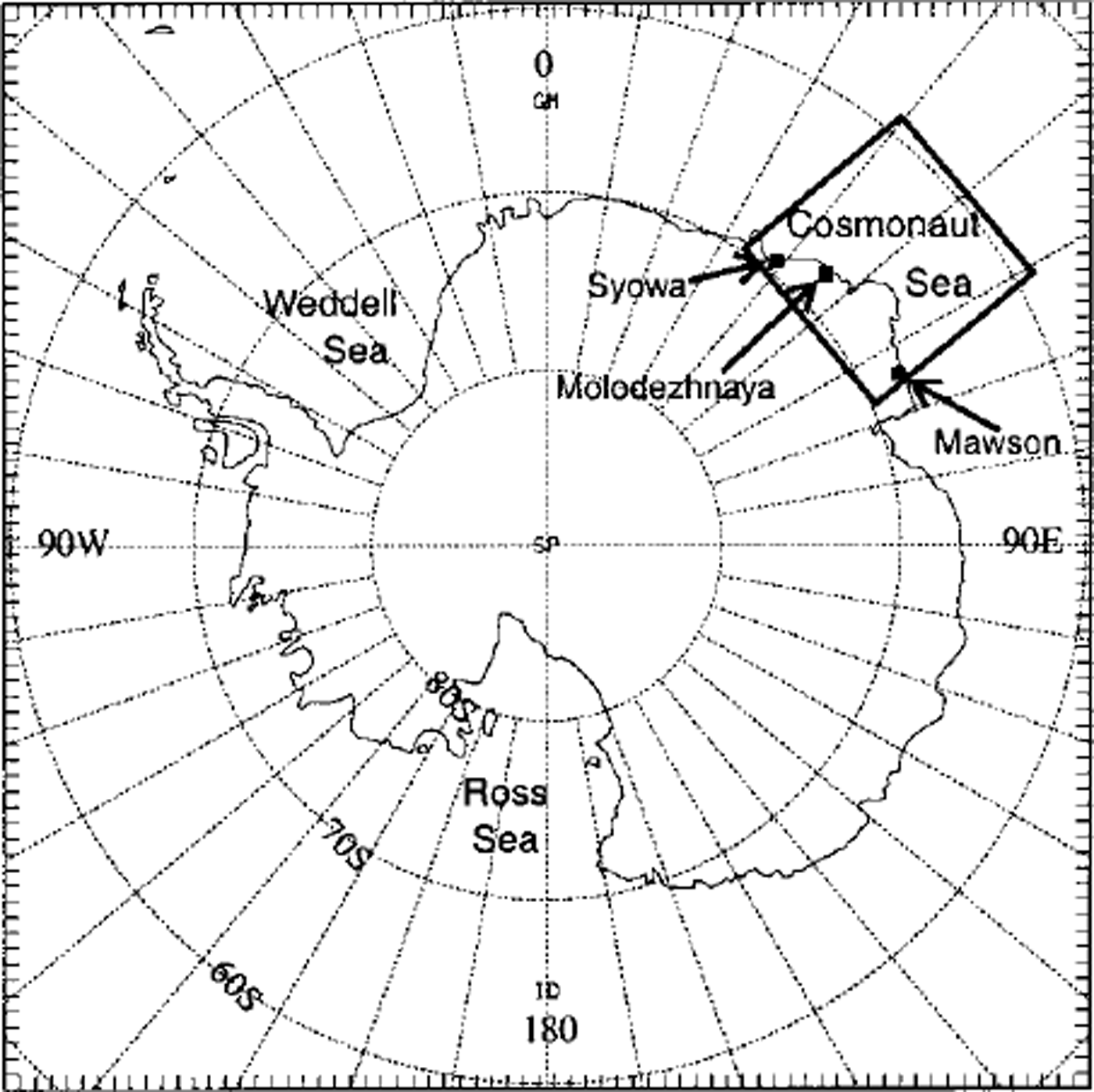
Fig. 1. Location of 20 km resolution Cosmonaut Sea domain, with the stations included m the domain.

Such polynyas involve complex interactions of the atmosphere-sea-ice-ocean system, the study of which is ideally suited to a coupled-model approach. This work presents a preliminary study of the Cosmonaut Sea region using an atmosphere-sea-ice model with prescribed deep-ocean heat flux, and, using a comparison with available satellite products and station data, will elucidate the strong influence of variable ocean-heat fluxes, and will evaluate the role of the atmosphere in the development of the winter sea-ice pack.

Model Description

As has been discussed, this type of phenomenon is well suited to a regional coupled-model approach which includes the interaction between the atmosphere-sea-ice-ocean system on higher resolutions than are possible with global models. The Antarctic Region Climate System Model (AntARCSyM) is a numerical model that includes comprehensive treatments of the atmosphere, ocean, sea ice and land surface for application over a limited region. AntARCSyM can be implemented at a range of grid resolutions (generally 10–100 km) and locations. This model has been adapted from the regional climate system model of the Arctic (ARCSyM), which has been used for simulations of the regional climate of Alaska (Lynch and others, 1995,1998,1999), in studies of the effects of the oceanic mixed layer and ocean circulation in the Beaufort Sea (Bailey and others, 1997), in studies of polynya formation in the Bering Strait (Lynch and others, 1997), in the analysis of sea-ice anomalies in the Arctic Ocean (Maslanik and others, 2000) and in investigations of clouds and radiation (Pinto and others, 1999). In the Antarctic region (Bailey and Lynch, 2000a, b), AntARCSyM has been shown to perform comparably to other limited-area atmospheric models (e.g. Walsh and McGregor, 1996; Hines and others, 1997a, b) which have fewer degrees of freedom than AntARCSyM.

ARCSyM has been described in detail in Lynch and others (1995); only a brief summary is given here. The atmospheric component is based on the NCAR RegCM2 (Giorgi and others, 1993a, b), a hydrostatic, primitive equation model with a terrain-following vertical coordinate and a staggered ’Arakawa B" horizontal grid. The sea-ice component used for this study is based on the elastic-viscous-plastic rheology of Hunke and Dukowicz (1997) and the thermodynamics of Parkinson and Washington (1979). The thermodynamics formulation is a simple two-layer model allowing for ice, open water and snow cover. The turbulent-heat and moisture fluxes are parameterized using the standard bulk aerodynamic formulae, with the turbulent transfer coefficient a function of the near-surface atmospheric stability. The bulk Richardson number is calculated separately over ice and open-water surfaces as a measure of the stability of the near-surface environment (Ebert and Curry, 1993). To our knowledge, there are no estimates of oceanic heat flux in the Cosmonaut Sea, and hence the seasonally varying oceanic heat flux prescribed from estimates for Prydz Bay from Heil and others (1996) is used with the standard mixed-layer formulation of Parkinson and Washington (1979). For the purposes of this sensitivity study, this specification is considered adequate, and is a small advance on the direct-tuning method of many models (e.g. Wu and others, 1996a), although clearly the use of an interactive ocean model is more desirable.

AntARCSyM is forced at the lateral boundaries using temperature, wind, moisture, surface-pressure and height fields, which may be provided from either observational analyses or output from a global climate model, and are updated every 6 or 12 h at every vertical level. The grid spacing of the model can be chosen depending on the application, and output from one AntARCSyM run can be used as lateral forcing for a higher-resolution AntARCSyM run over a smaller domain, in one-way nested mode. The AntARCSyM can be run with any combination of surface models, with boundary conditions specified for the remaining components (eg. atmosphere-ice-land with specified sea-surface temperatures). In this way the influence of each component can be evaluated independently.

Data and Experiment Description

Considerable data are available for various parts of the Antarctic region, which have been used for initial model evaluation and testing (Bailey and Lynch, 2000a, b). Antarctic station and upper-air data for all of the U.S. automatic weather-station (AWS) systems as well as radiosonde launches at several international stations around the continent for 1988–89, including Molodezhnaya, were obtained from the University of Wisconsin. Additional Australian station and upper-air data for Mawson were obtained from the Australian Bureau of Meteorology (BMRC), and station and upper-air data at the Japanese base (Syowa) were obtained from the National Institute of Polar Research (NIPR). Passive microwave (SSM/I) sea-ice concentrations were obtained from the U.S. National Snow and Ice Data Center.

The simulation considered here is a 20 km resolution domain centred at 65° S, 50° E (see Fig. 1) which contains three Antarctic stations at Syowa, Molodezhnaya and Mawson. The results of the simulation shown here are for July 1988, after 1 month of spin-up, driven by 12 hourly European Centre for Medium-range Weather Forecasts (ECMWF) forcing (interpolated to 20 km resolution) at the boundaries. The model sea ice was initialized on 1 June using the SSM/I-derived sea-ice concentration with a uniform thickness of 50 cm, and the atmospheric fields with the interpolated ECMWF analyses. The sea-surface temperatures were initialized using the climatology of Shea and others (1992). The model fields were compared to the analyses and available observed data.

Results

Figure 2 presents a comparison of the mean July sea-ice concentration from SSM/I and the model. The continental topography is included for orientation. The model sea-ice concentration is higher throughout the domain with a larger sea-ice extent. While the SSM/ I product may be underestimated by up to 5% (personal communication from J. A. Maslanik, 1998), there remains a significant bias. The model shows reduced concentration only in the coastal areas where the sea ice is removed by the continental winds.

Fig. 2. Mean July 1988 sea-ice concentration: (a) SSM/I-derived and (b) model-simulated.

Figure 3 shows a comparison of the lowest-sigma-level (about 40m height) mean July atmospheric temperature from the ECMWF analyses (Fig. 3a) and the model simulation (Fig. 3b). (The continental topography is included for orientation.) The model does not have a clear bias compared to the analyses, with an rms difference of 1.4 K. The model and analyses differ (Fig. 3c) up to ±4 K. These differences are expected as the analyses have been interpolated down to 20 km, whereas the model simulation is performed at 20 km.

Fig. 3. Mean July 1988 lowest-sigma-level atmospheric temperature (K)for (a) ECMWF analyses, (b) model simulation and ( c) model minus analyses.

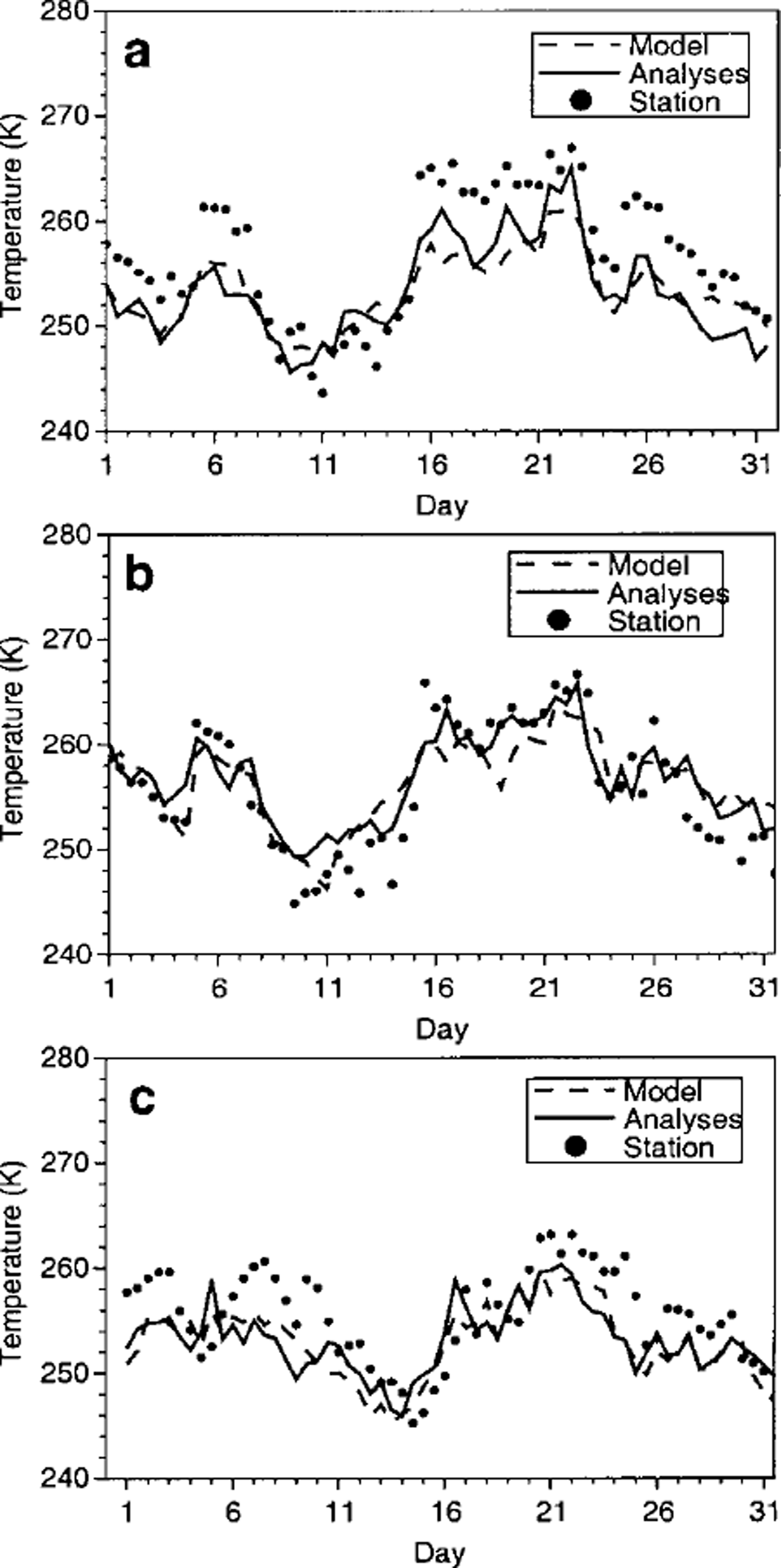
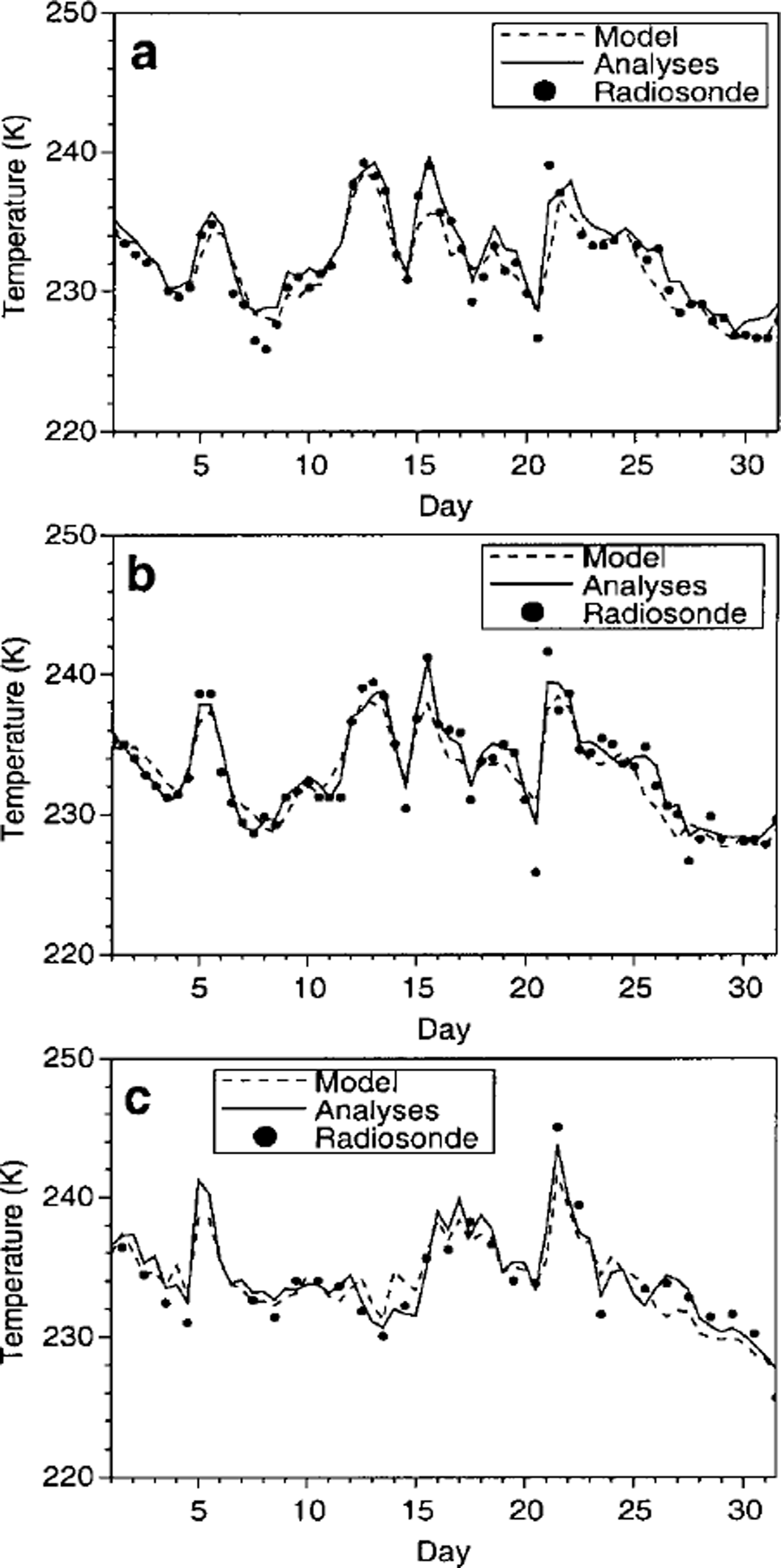
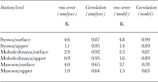
More importantly, consider a simple comparison of the ECMWF analyses and model temperatures with station data (Fig. 4) and radiosonde launches (Fig. 5) in the region. The root-mean-square (rms) errors and correlation coefficients are shown in Table 1. Notice that the upper-air agreement (Fig. 5) is much better at all stations than the surface-air agreement(Fig. 4) for both the model and analyses. The correlation coefficients are much lower for the upper-air Mawson comparison as a number of the radiosonde launches were missing. This is typical in model simulations of Antarctica, where most of the bias is found near the surface (Bailey and Lynch, 2000b). In general the analyses show lower rms errors and higher correlation coefficients than the model simulations when compared to the stations. While this is true for these coastal stations, the comparisons of Bailey and Lynch (2000b) showed that this is not generally true over the whole continent. Also, the quality of the analyses over the ocean is unknown due to lack of observations. Generally, the ECMWF analyses do capture the large-scale features and compare well with the stations because of the data-assimilation scheme which produces the analyses.

Fig. 4. Mean July surface-air temperature (K) comparison at (a) Syowa, (b) Molodezhnaya and (c) Mawson.

Fig. 5. Mean July upper-air (500 mb) temperature (K) comparison at (a) Syowa, (b) Molodezhnaya and (c) Mawson.

Table 1. Summary of analyses and model-to-station comparison

There is no clear warm or cold bias in the model simulations compared to the analyses and stations, yet the sea-ice concentration and extent are larger than in the SSM/ I-derived product. This implies that there must be another source of heat to melt the sea ice in this region, which must come from the ocean.

Summary and Discussion

The sea-ice concentration and extent are overestimated in the model when compared to the SSM/I-derived product. Despite a possible underestimation from the SSM/I, this would seem to be a real bias. Given the good level of skill in simulating the atmospheric conditions in this region (not shown; see Bailey and Lynch 2000a, b), based on the limited observations, this is attributed to a lack of heat from the ocean. This points to a need for the presence of upwelled Circumpolar Deep Water to provide a heat source to regulate the sea-ice cover in this region. Full continental simulations of the Antarctic with this model (Bailey and Lynch 2000a) show a much more realistic sea-ice distribution in the Cosmonaut Sea region, using the same oceanic heat-flux parameterization. So, while this parameterization is adequate at coarser resolution, it is not appropriate for all scales. If this approach is maintained, this implies a need to develop a new parameterization for each new domain of simulation.

The implication of this study is that the polynya in this region would not form in a model simulation under atmospheric forcing alone without a"tumng"⁰f the Parkinson and Washington (1979) oceanic heat flux. A better solution would be the incorporation of an interactive one-dimensional mixed-layer or three-dimensional primitive equation ocean model. Thus, oceanic processes provide the key to the formation and maintenance of the Cosmonaut polynya, which may still require atmospheric preconditioning. Work is underway to perform more sensitivity studies with the inclusion of these ocean components and evaluate the relative impacts of the atmosphere and ocean.