The extant literature is replete with studies of the effectiveness of generic advertising and promotion programs conducted by the already large and growing number of commodity “check-off” programs in the United States (e.g., Forker and Ward Reference Forker and Ward1993, Williams, Shumway, and Love Reference Williams, Shumway and Love2002, Kaiser et al. Reference Kaiser, Alston, Crespi and Sexton2005, Kaiser Reference Kaiser2006, Williams and Capps Reference Williams and Capps2006, Reference Williams and Capps2011, Williams, Capps, and Dang Reference Williams, Capps and Dang2010, Capps, Williams, and Málaga Reference Capps, Williams and Málaga2013, Capps et al. Reference Capps, Williams, Salin, Martini and Brown2013). Check-off programs are primarily cooperative efforts by producers of similar agricultural products to enhance their individual and collective profitability through advertising at the retail end of the supply chain. Virtually every U.S. agricultural commodity is associated with some type of organization dedicated to promoting the economic welfare of its producers through retail-level generic advertising programs funded through check-off fees imposed on sales by producers and sometimes others in the marketing chain. The term check-off comes from the concept of checking the appropriate box on a form such as a tax return to authorize a contribution for a specific purpose, such as public financing of election campaigns or, in this case, financing programs to enhance producer welfare.
Prior research on the effectiveness of generic advertising and promotion activities by U.S. commodity check-off programs has focused primarily on deriving stakeholders’ returns on investment or on benefit-cost ratios. The methodological thread common to the studies is a comparison of the results of two simulations: (i) a baseline “with promotion expenditures” scenario using actual expenditures in a period and (ii) a counterfactual “without promotion expenditures” scenario that eliminates the program by setting its expenditures to zero during the same period.Footnote 1
The counterfactual is rarely realized in practice, but in 2001 the Florida Department of Citrus (FDOC), which was responsible for virtually all of the orange juice industry's national generic advertising, went “nearly dark” when it almost completely defunded its massive program promoting orange juice for three months. We take advantage of this natural experiment to estimate the resulting loss in national consumption and sales revenue during that period. We also examine the length of time required for sales and consumption of orange juice to recover once the FDOC reversed its decision. Our analysis makes use of both a structural econometric model and a vector autoregression model of orange juice advertising. Consequently, our work adds to the literature by analyzing the consequences of a generic advertising program nearly going dark using alternative quantitative approaches.
The only other study that has addressed this situation is Crespi and Sexton (Reference Crespi, Sexton, Kaiser, Alston, Crespi and Sexton2005), which evaluated the effectiveness of promotion by the California Almond Board. The board's entire advertising program was suspended for three crop years (1994/95 through 1996/97) due to litigation. Crespi and Sexton (Reference Crespi, Sexton, Kaiser, Alston, Crespi and Sexton2005, p. 168) found that “the almond industry in California suffered substantially in terms of profits due to the suspension of the industry advertising program imposed by litigation,” costing the industry an accumulated profit that was estimated at between $84 million and $231 million.
The implications of this work are important for several reasons. First, funding for such check-off programs derives from sales of agricultural commodities and thus is susceptible to year-to-year variability. If, for example, funding is reduced by weather-related crop shortfalls, the effect of the lack of promotion on retail demand can extend into subsequent years. In addition, producers opposed to paying check-off assessments continually challenge the validity and effectiveness of the programs, often in court (Crespi and Sexton Reference Crespi and Sexton2001, Crespi Reference Crespi2003). Our study can elucidate the potential consequences of defunding a check-off program.
Methodology
To examine the repercussions of FDOC's nearly going dark from September 2001 through November 2001, we econometrically estimate the coefficients of a structural representation of U.S. retail demand for orange juice for January 1989 through August 2001. The estimated demand model is then used to forecast per capita consumption in the United States for September 2001 through September 2002. By calculating the difference between actual and forecasted per capita consumption, we can estimate foregone total consumption and sales of orange juice as a result of the lack of promotion.
To check the robustness of the findings, we employ vector autoregression to isolate the effects of FDOC advertising. This check is especially important since measurements of advertising impacts depend heavily on the ability to monitor carryover effects. That is, both contemporaneous (current) and lagged (past) advertising expenditures must be accounted for in the analysis.
From the time-series analysis, we calculate a historical partition of orange juice consumption at any date T + k into the information available at time t = T and the information revealed at period t = T + 1, T + 2, … , T + k. This partition depends on a linear combination of historical innovations from each variable indigenous to the vector autoregression. Based on information known in August 2001, we make monthly forecasts through September 2002. At each forecast date, the difference between actual and forecasted orange juice consumption is expressed as a function of the variables in the vector autoregression.
Though the length of the suspension is short (September through November 2001), it has no bearing on our analysis. It corresponds to the out-of-sample period so the estimated coefficients from the models are not affected by the nearly-going-dark period. Our methodology is particularly suited to the objective of determining the repercussions of the FDOC's program hiatus. A modified post-estimation analysis that depends on including the full sample period to estimate the respective coefficients of the models would co-mingle data from before and after the nearly-going-dark period, thus reflecting a mixture of effects and prohibiting the ability to determine the ramifications of nearly going dark statistically.
Structural Econometric Model
From economic theory, the primary drivers of demand for a product are (i) inflation-adjusted prices, (ii) prices of substitutes and/or complements, (iii) disposable personal income, (iv) advertising expenditures (in this case, both generic FDOC and brand advertising expenditures on orange juice and on competing fruit juices and drinks), and (v) seasonality given our use of intra-year (monthly) data in the analysis.
Our structural specification of the demand function for orange juice is consistent with the literature on demand for nonalcoholic beverages (e.g., Zheng and Kaiser Reference Zheng and Kaiser2008) and can be expressed as
where
q t = gallons (per capita) of orange juice consumed in period t where the per capita consumption in period t is total U.S. consumption divided by the U.S. population in period t.
p t = the real U.S. price of orange juice in period t: nominal orange juice price in period t deflated by the U.S. consumer price index (CPI) for nonalcoholic beverages in period t.
p st = the real U.S. price of grapefruit juice (the nominal price of grapefruit juice deflated by the CPI for nonalcoholic beverages in period t) as a substitute for orange juice. The prices of other nonalcoholic beverages are accounted for through use of the CPI, thus circumventing potential collinearity among prices of the numerous other potential substitute beverages.
y t = real U.S. disposable personal income per capita in period t: total U.S. disposable personal income divided by the population in period t and then divided by the CPI for all items.
FOJA t = real advertising expenditures for orange juice by FDOC in period t: nominal expenditures deflated by the CPI.
BOJA t = real brand advertising expenditures for orange juice in period t: nominal expenditures deflated by the CPI.
FJDA t = real advertising expenditures on fruit juices and drinks, excluding orange juice, in period t: nominal expenditures deflated by the CPI.
Seasonality is accounted for using a set of monthly indicator (0–1) variables.
This specification, which includes three measures of advertising effort, has not typically been used to analyze generic advertising. The variable FOJA t represents generic advertising and promotion activities by FDOC. However, numerous brands promote their orange juice products through substantial advertising campaigns. Generic advertising is often thought to increase the “size of the pie” and brand advertising to primarily alter the brand's “share of the pie,” but some studies have found evidence of interaction effects between the two types of advertising (e.g., Brester and Schroeder Reference Brester and Schroeder1995, Kaiser and Liu Reference Kaiser and Liu1998, Chakravarti and Janiszewski Reference Chakravarti and Janiszewski2004, Isariyawongse, Kudo, and Tremblay Reference Isariyawongse, Kudo and Tremblay2007). Consequently, BOJA t is included to account for the potential interaction effects of brand advertising. The variable FJDA t, which represents advertising of other fruit juices and drinks, is included to account for potential “beggar thy neighbor” effects of advertising by substitute products (Alston, Freebairn, and James Reference Alston, Freebairn and James2001).
We adopt a double logarithmic form of equation 1 to insure diminishing marginal returns, which are normally associated with advertising efforts. Comparable granular data on demand for nonalcoholic beverages were not available for a demand system analysis. Therefore, we do not capture inter-relationships among nonalcoholic beverages that may affect the magnitude of the impact of nearly going dark on consumer sales.
A Hausman test was employed to check for potential endogeneity of the real price of orange juice. It revealed that the real price of orange juice was indeed exogenous. Consequently, a single-equation specification was deemed appropriate.
Time-series Model
An alternative model for the econometric (structural) representation of the demand function is a time series. According to Sims (Reference Sims1980), equation 2 represents multiple economic time series in which lags (determined from the data and a priori knowledge) of each variable are allowed (in the most general case) to affect the current position of each series. The resulting model can be specified as a vector autoregressive representation (VAR):
 $$x_t = \sum\limits_{k = 1}^K {{\rm \alpha} \lpar k \rpar x_{t - k} + {\bf e}_t} $$
where α(k) is an autoregressive matrix of the dimension (n × n) at lag k that connects x t and x t–k, n represents the number of endogenous variables included in the vector autoregression, and et is a vector residual term of dimension (n × 1).
Most of the autoregressive parameters, α(k), equal zero and K is the maximum lag found through the loss-function search procedures. By moving all of the terms involving x t and x t–k to the lefthand side of the VAR and expressing the lags in terms of the lag operator (B), we can specify an autoregressive representation:
Merely inverting the autoregressive representation to the righthand side gives us the standard moving-average representation:
which can be written in more discernable terms as an infinite sum:
where π(i) represents matrices of the moving-average parameters (n × n) derived from the VAR equation and e t–i represents vectors of historical shocks of dimension (n × 1).
The structure of the VAR equation allows a decomposition of the x vector at t into its historical components. For any particular element of x t, say element i, we can write this expression as
 $$x_{it} = e_t + \sum\limits_{\,j = 1}^n {{\rm \pi} _{ij} \lpar 1 \rpar e_{\,jt - 1} +} \sum\limits_{\,j = 1}^n {{\rm \pi} _{ij} \lpar 2 \rpar e_{\,jt - 2} +\ldots }$$
where e t–k is the shock in series j in period t – k and πij(k) is the i, j element of the π matrix of the moving-average parameter matrix that gives the response of series i to the shock in period t – k in series x j. At any time t, we can determine the portion of the series associated with past shocks in any of the particular series (j) of the vector time series.
Historical decompositions of time-series models are not independent of the ordering of contemporaneous correlation. In this analysis, the causal flows in contemporaneous time are investigated using the directed graph procedures of Spirtes, Glymour, and Scheines (Reference Spirtes, Glymour and Scheines2000) and Swanson and Granger (Reference Swanson and Granger1997). Such methods allow for use of a nonrecursive ordering of contemporaneous correlation that avoids much of the criticism leveled at VAR work conducted with the standard Cholesky factorization (Cooley and LeRoy Reference Cooley and LeRoy1985). In this study, the historical decompositions allow us to examine movements in monthly consumption of orange juice in response to historical shocks associated with real FDOC advertising expenditures, brand advertising expenditures on orange juice, advertising expenditures on fruit juices and drinks other than orange juice, prices of orange and grapefruit juice, and per capita income.
Data
Table 1 describes the source of each type of data (sales, consumption, and advertising) and presents descriptive statistics associated with the variables used in the econometric and vector autoregression models before, during, and after the nearly-dark period. We obtained scanner data from Nielsen for January 7, 1989, through September 28, 2002, on weekly dollar sales, gallons sold, and price per gallon of orange juice and grapefruit juice. That data, however, did not align with the monthly periodicity of data on real disposable incomes, the U.S. population, the general CPI, the CPI for nonalcoholic beverages, or any of the measures of advertising expenditures. To match the periodicity of these variables, we adjusted the weekly Nielsen scanner data to monthly figures. The nominal prices of orange and grapefruit juices were adjusted for inflation using the seasonally adjusted series from the CPI for nonalcoholic beverages, and the nominal per-capita income and the respective nominal advertising variables were adjusted for inflation using the seasonally adjusted CPI series.
Table 1. Descriptive Statistics of the Variables, January 1989 through September 2002

Traditional Nielsen scanner data sets pertain to retail supermarkets for which sales exceed $2 million per year. Nielsen also provided additional data for supercenters plus Wal-Mart but only for September 1996 through September 2002, so further adjustments were made to combine the scanner data with the information from retail supermarkets. Consequently, monthly observations pertaining to nominal and real U.S. sales, consumption quantities, and prices for orange juice and grapefruit juice for January 1989 through September 2002 were available for analysis.
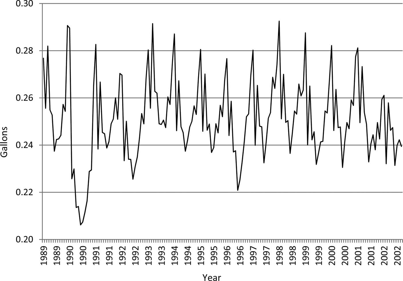
On average during the sample period, per capita consumption of orange juice was slightly more than 0.25 gallons per month and ranged from 0.20 to 0.30 gallons per month. Seasonality is clearly evident (see Figure 1). The mean nominal price of orange juice was $3.88 per gallon and the mean nominal price of grapefruit juice was $4.47 per gallon. The average for annual nominal per-capita income was $21,064 and ranged from $15,957 to $27,456.

Figure 1. U.S. Per Capita Orange Juice Consumption, January 1989 through September 2002
In the analysis of the effects of advertising on demand for orange juice, advertising effort is measured by the dollar amounts spent on FDOC and brand advertising of orange juice and on advertising of other fruit juices and drinks provided by Competitive Media Reporting (CMR) through the Richards Group, an advertising agency in Dallas, Texas. The CMR data set reports advertising expenditures for a variety of media categories, including magazines, Sunday magazines, newspapers, billboards, network television, spot television, syndicated television, cable television networks, network radio, and national spot radio. We aggregated the individual categories into total advertising dollars for the analysis.
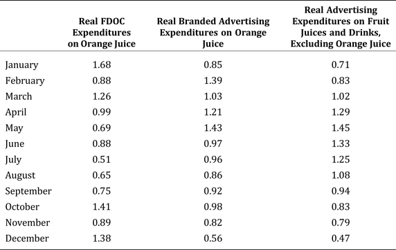
As shown in Table 1, FDOC's average nominal monthly expenditure for advertising was roughly $1.80 million and varied between $2,300 and $7.0 million over the sample period. Its real advertising expenditures were greatest in January, March, October, and December and least in May, July, August, and September. This seasonal pattern is similar to the seasonal pattern typical of consumption of orange juice.
In terms of brand advertising, the average nominal monthly expenditure was slightly less than $4.74 million over the sample period, about 2.6 times that of FDOC's (Table 1). The monthly expenditures ranged from $190,700 to almost $14.39 million. The top three brands accounted for about 88 percent of the average expenditure: Tropicana, 46.2 percent; Minute Maid, 24.8 percent; and Florida's Natural, 16.7 percent.
On average over the study period, branded advertising expenditures accounted for roughly 72 percent of total advertising of orange juice in the United States compared to 28 percent by FDOC. Like FDOC's advertising expenditures, branded advertising exhibited seasonal variations but the pattern was markedly different from that of FDOC. The branded advertising expenditures were greatest in February, April, and May and least in January, August, November, and December.
The nominal monthly advertising expenditures for all fruit juices other than orange juice averaged roughly $16.57 million and varied between $3.99 million and $36.86 million over the sample period. This category included apple juice, grape juice, cranberry juice, grapefruit juice, and other citrus juice products.
Because seasonality was evident in the advertising expenditures for FDOC, brands, and other fruit juices, we constructed seasonal adjustments for these variables using the X12 procedure from the U.S. Census Bureau. Those factors are presented in Table 2.
Table 2. Seasonal Factors Related to Advertising Expenditures

Note: Seasonal factors were obtained using the software package EViews 7.1 based on the X12 procedure from the U.S. Bureau of the Census.
Empirical Results
As previously noted, monthly data for January 1989 through August 2001 are used in the model estimation, and the monthly observations for September 2001 through September 2002 are withheld to assess the effects of nearly going dark.
Results of the Structural Econometric Model
Previous research has established that advertising has carryover or lagged effects (e.g., Nerlove and Waugh Reference Nerlove and Waugh1961, Waugh Reference Waugh1959, Ward and Lambert Reference Ward and Lambert1993, Ward and Dixon Reference Ward and Dixon1989, Wohlgenant and Clary Reference Wohlgenant and Clary1992). However, neither economic theory nor previous research has provided much guidance regarding the appropriate structure and duration of the dynamic processes involved. Conventionally, researchers have relied on the data in choosing the optimal number of lags to include when specifying a particular advertising stock variable using statistical criteria such as the Akaike information criterion (AIC), the Schwarz information criterion (SIC), and the Hannan-Quinn criterion (HQC). The coefficients associated with the contemporaneous and lagged advertising expenditures also are commonly assumed to be free-form lags or to follow some type of distribution, such as a geometric decay or a polynomial (Almon) distributed lag. Piggott et al. (Reference Piggott, Chalfant, Alston and Griffith1996) treated the advertising process as a free-form lag of four quarters. Cox (Reference Cox1992) and Brester and Schroeder (Reference Brester and Schroeder1995) used a second-order exponential lag distribution while Baye, Jansen, and Lee (Reference Baye, Jansen and Lee1992) employed a geometric lag. Williams, Shumway, and Love (Reference Williams, Shumway and Love2002) used a polynomial inverse lag. Kaiser (Reference Kaiser2006) in an investigation of demand for eggs, Williams and Capps (Reference Williams and Capps2011) in an investigation of demand for cotton, and Capps et al. (Reference Capps, Williams and Málaga2013) in an investigation of demand for fluid milk, cheese, and butter used polynomial distributed lags with endpoint restrictions.
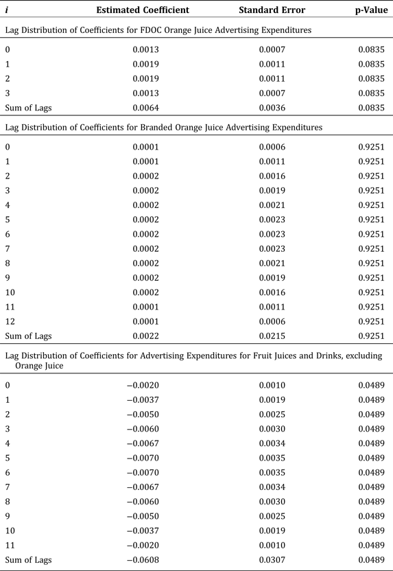
To characterize the carryover effects of advertising in this analysis, we use a second-degree polynomial (Almon) distributed lag with head and tail restrictions. With these restrictions and use of a second-degree polynomial lag, we only need to estimate a single coefficient associated with each of the three advertising expenditure variables. The estimation process allows for a minimum of two lags and a maximum of twelve lags in the carryover advertising responses. Experts in the U.S. citrus industry suggested using twelve lags, and use of the maximum lag length was supported by the literature on estimation of demand models with advertising effects. In an often-cited study, Clarke (Reference Clarke1976) concluded that 90 percent of the cumulative effects of advertising for frequently purchased products are captured within three to nine months. Identifying the optimal lag length for the three types of advertising expenditures collectively required estimation of 1,331 (113) alternative structural models to account for each possible permutation of lags. Thus, we chose the final structural specification to minimize the SIC statistic.
We use an indicator variable, SCO996, to represent a structural change in our data set for consumption of orange juice (gallons sold). From January 1989 through August 1996, only retail supermarkets are included; thereafter, the data set covers both retail supermarkets and mass merchandisers. The indicator variable equals 1 for monthly observations after August 1996 and 0 otherwise.
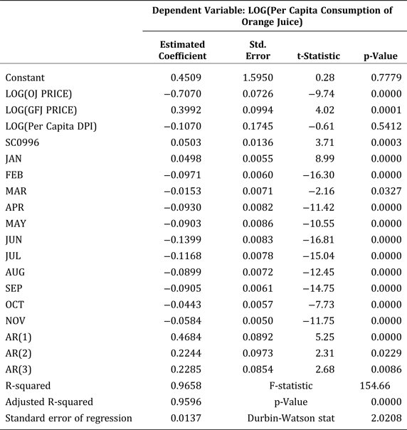
Table 3 presents the results of the structural econometric model for the period preceding FDOC's promotion hiatus (January 1989 through August 2001), leaving observations for September 2001 through September 2002 as out-of-sample predictions to assess orange juice consumption after the nearly-going-dark period. The level of significance chosen for this analysis is 0.05, and the reported p-values correspond to probability values associated with two-tailed t-tests. The appropriate p-values for one-tailed tests are half of the reported probability values.
Table 3a. Empirical Results of the Econometric Structural Model Using Data from January 1989 through August 2001

Table 3b. Empirical Results of the Econometric Structural Model Using Data from January 1989 through August 2001: Lag Distributions

We estimate the demand model using generalized least squares in which the residuals exhibit a third-order autoregressive process using EViews version 8.0 software. We find that about 96 percent of the variability in per capita consumption of orange juice is explained by the model. Significant drivers of demand for orange juice are the real price of orange juice (own-price elasticity of –0.707), the real price of grapefruit juice (cross-price elasticity of 0.399), real expenditures for FDOC generic advertising, real expenditures for advertising of fruit juices and drinks other than orange juice, seasonality, and the structural-change factor.
FDOC's generic advertising expenditures significantly shift the orange-juice demand curve outward. The optimal lag length associated with its advertising effort is three months. The cumulative advertising elasticity is 0.0064 so that a doubling of its advertising expenditures yields a 0.64 percent increase in monthly per-capita consumption. The cumulative (long-run) effect of FDOC's advertising is relatively small.
In contrast, expenditures for advertising of branded orange juice are found to have no statistically significant impact on monthly per-capita consumption of orange juice, a result that is consistent with Brown and Lee (Reference Brown and Lee1997, Reference Brown and Lee1999) and Brown (Reference Brown and Lee2002). The estimated optimal lag length is twelve months, and the cumulative advertising elasticity is 0.0022. This coefficient is not statistically different from zero, which suggests that generic advertising is more effective than branded advertising at increasing consumption of orange juice.
However, branded advertising may have maintained some of the demand for orange juice in the near absence of generic advertising. To analyze this possibility, we calculate sample means for the generic and branded advertising expenditures prior to, during, and after the roll-back period. In the near absence of generic advertising, the nominal branded advertising expenditure is 7 percent higher on average than the average brand expenditure prior to the roll-back. After FDOC's advertising resumed, the average nominal expenditure for branded advertising remains nearly 2 percent higher than prior to the roll-back. As noted, FDOC's advertising expenditures were nearly zero during the blackout; after FDOC resumed promotions, its average nominal expenditure for generic advertising was 66 percent higher than prior to nearly going dark.
A unique feature of our analysis is consideration of the impacts of three types of advertising: generic advertising by FDOC; branded advertising predominantly by Tropicana, Minute Maid, and Florida's Natural; and advertising of fruit juices and drinks other than orange juice. Expenditures on advertising of fruit juices and drinks other than orange juice negatively affect monthly per-capita consumption of orange juice as expected. The cumulative cross-advertising elasticity is statistically significant at –0.0608. The optimal lag length is eleven months. We find that this cross-advertising elasticity is larger in absolute value than the own-advertising elasticity. This result does not conflict with economic theory.
Seasonality is evident from the analysis of monthly consumption of orange juice. Per capita consumption for January is roughly 5.1 percent higher than consumption for the base/reference month of December and is lower than December's consumption for all other months. The difference ranges from 1.4 percent in March to 12.9 percent in June. The estimates are consistent with the descriptive statistics; consumption is greatest in January and December and lowest in June and July.
The addition of supercenters and Wal-Mart to the monthly data after August 1996 yields roughly a 5.2 percent increase in per capita consumption of orange juice when all other factors remain the same. Disposable income does not statistically affect consumption.
Results of the Vector Autoregression Model
The seven-equation vector autoregression model involves the same variables as the econometric analysis, including per capita consumption and the real price of orange juice, the price of grapefruit juice, per capita disposable income, FDOC and branded advertising expenditures on orange juice, and advertising expenditures for other fruit juices. As in the structural model, we use monthly indicator variables to account for seasonality.
Initially, we examined the stationarity of the respective series using augmented Dickey-Fuller tests (Dickey and Fuller Reference Dickey and Fuller1981) and found that the real price of orange juice, real price of grapefruit juice, and per capita disposable income were nonstationary series. Per capita consumption of orange juice, real FDOC advertising expenditures, real branded advertising expenditures, and real advertising expenditures for other fruit juices were stationary. Based on Beaulieu and Miron (Reference Beaulieu and Miron1993), we determined that seasonal nonstationary behavior was not evident in any of the series. Additional information regarding the tests of nonstationarity are available from the authors upon request.
Based on the stationarity tests, we specified the vector autoregression equations for per capita orange juice consumption, real FDOC advertising expenditures for orange juice, branded advertising expenditures for orange juice, and advertising expenditures for other fruit juices in levels. The equations pertaining to the prices and per capita income were specified in first differences.
The number of lags to include in the model was determined from the data. We used the SIC (also known as the Schwarz-loss criterion) and the AIC to determine the lags, t – k, for k = 1, 2, … , 6 (Geweke and Meese Reference Geweke and Meese1981). In addition to identifying the lag length, the two loss functions (SIC and AIC) were used to determine whether seasonal dummy variables should be included. Based on these metrics, we determined that the best model was a vector autoregression with a one-period lag and seasonal dummy variables. Equation 7 is a general statement of the optimal model according to the SIC and AIC.
 $$X_i \lpar t \rpar = {\rm \mu} _i + \sum\limits_{j = 1}^{11} {{\rm \delta} _{ij} D_j} + \sum\limits_{k = 1}^7 {B_{ik} X_k \lpar {t - 1} \rpar } + e_i \lpar t \rpar \quad i = 1\comma \; 2\comma \; . . . \comma \; 7$$
Each series (X i) in period t depends on a constant (μi); eleven monthly dummy (indicator) variables (D j) for j = 1, 2, … , 11; one lag for each of the seven variables (including itself); and a current-period error (innovation) term, e i(t).
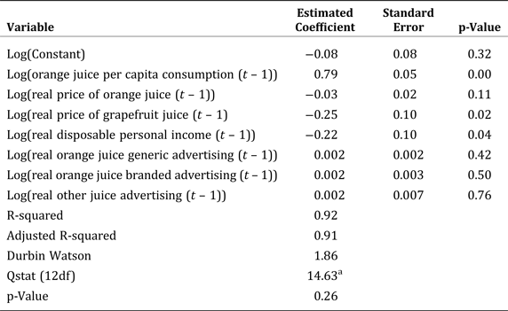
Table 4 presents the estimated coefficients, standard errors, and goodness-of-fit statistics for the equation that specifies per capita consumption of orange juice. Significant coefficients are obtained for lagged per capita consumption, real price of orange juice, real price of grapefruit juice, and real per capita disposable income and for the set of seasonal indicator variables. Based on use of Ljung-Box Q-statistics, we find that the residuals associated with the per-capita orange-juice-consumption equation exhibit no serial correlation at conventional levels of significance. The parameter estimates, standard errors, and p-values associated with this autoregression model are available from the authors upon request.
Table 4. Empirical Results for the Consumption Equation from the Autoregression Model Using Data for January 1989 through August 2001

a Ljung-Box Q-statistics check for the presence of serial correlation.
Notes: The parameter estimates, standard errors, and p-values of the remaining equations from the model are available from the authors upon request. Indicator variable coefficients and statistics are not reported due to space limitations.
To account for innovation, the contemporaneous structure of the error covariance must be orthogonal, a condition that cannot generally be met. To obtain orthogonal innovations, we use a Bernanke ordering (Bernanke Reference Bernanke1985) in lieu of a Choleski ordering (Lütkepohl Reference Lütkepohl1991) since the Choleski decomposition may not reflect the true causal pattern for a set of contemporaneous innovations (Park, Jin, and Bessler Reference Park, Jin and Bessler2008). Furthermore, we apply a directed acyclic graph (DAG) identified using an algorithm developed by Spirtes, Glymour, and Scheines (Reference Spirtes, Glymour and Scheines2000) to identify vector autoregression innovations (Swanson and Granger Reference Swanson and Granger1997, Haigh and Bessler Reference Haigh and Bessler2004, Awokuse and Bessler Reference Awokuse and Bessler2003, Hoover Reference Hoover2005, Attavanich, McCarl, and Bessler Reference Attavanich, McCarl and Bessler2011). Details are available from the authors.
With the algorithm-DAG causal inference method, one can explore dynamic interactions among the variables in a model using various types of innovation-accounting analyses, the main ones being impulse response functions, forecast error-variance decompositions, and historical decompositions. The forecasted error decompositions summarize the relative importance of each variable to itself and the other variables in the model. Impulse responses summarize the dynamic pattern of movement of each variable in response to a shock in a particular variable.
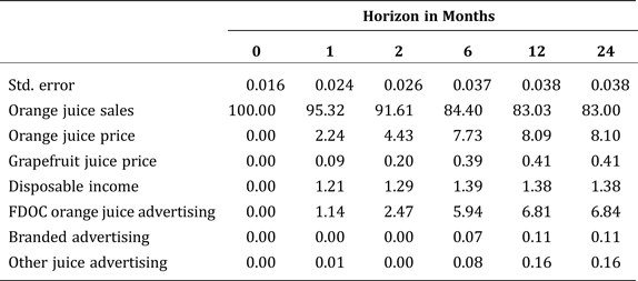
Our primary interest is in the forecasted decomposition of the error variance for per capita orange juice consumption that is associated with the one-lag model. Those results for data for January 1989 through August 2001 are presented in Table 5. The decompositions show the relative importance of each variable in the seven-equation system to itself and to the other six variables for five forecast horizons: one, two, six, twelve, and twenty-four months ahead. The sum of all numbers in a column must be 100 but for rounding error. When a large percentage appears in a row, the row variable is identified as an important influence on consumption of orange juice. At horizons of one and two months, the real price of orange juice and real FDOC advertising expenditures begin to influence per capita consumption. This influence persists through the two-year horizon. Real per capita income appears to have a moderate influence at best on consumption of orange juice. The real price of grapefruit juice, branded advertising expenditures, and expenditures to advertise other fruit juices exert weak influences on consumption of orange juice.
Table 5. Forecasted Error-variance Decomposition on Per Capita Orange Juice Consumption, January 1989 through August 2001

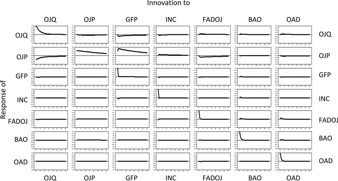
We normalize the impulse response of each series to a one-time-only shock by dividing each response by the historical standard deviation of its vector autoregression error (innovation) term (see Figure 2), placing each response on the same relative scale (–1, +1). The responses shown in the rows in Figure 2 are for 36 monthly periods following an initial one-time-only shock in the variable listed at the top of each column. Because the responses are normalized, it is legitimate to compare the graphs without regard to units of measurement. Presenting all of the graphs in a single figure demonstrates the dynamic structure of the responses in a relative sense.

Figure 2. Response of Vector Autoregression System with One-period Lag to a One-time-only Shock in Each Variable Using Data for January 1989 through August 2001
Figure 2 shows that all of the dynamics are essentially worked out within twelve months. In addition, the most important variable associated with per capita consumption of orange juice is its own shock, which is positive and equals one historical standard deviation in innovation (error) from the model.
The second most important variable in the dynamic behavior of consumption is the real price of orange juice. That response, in accord with expectations, is negative and peaks five months after the shock. Thereafter, the consumption response declines in a manner resembling a geometric decay and drops to zero in twelve months.
The third most important dynamic influence on orange juice consumption is real FDOC advertising expenditures. The consumption response is positive, as expected, for the first six months following the shock; subsequent relative responses decline and approach zero (consumption returns to its pre-shock level). The peak occurs in months three through six.
The elasticity of per capita consumption of orange juice with respect to real FDOC advertising expenditures after all of the dynamics have played out (after twelve months) is comparable to the cumulative advertising elasticity gleaned from the econometric model. The responses of orange juice consumption to shocks in branded advertising expenditures, advertising expenditures for other fruit juices, per capita income, and price of grapefruit juice essentially are negligible.
Econometric Analysis of the Repercussions of Nearly Going Dark
As previously discussed, FDOC expenditures on advertising of orange juice declined almost to zero in the latter part of 2001. Specifically, the nominal advertising expenditures were $13,000 in September, $2,300 in October, and $5,200 in November, well below the average of $1.8 million per month from January 1989 through September 2002. FDOC reinstated its promotion program in January 2002 and advertising expenditures gradually increased to $698,200 in July 2002 and to $7,012,200 in January 2003.
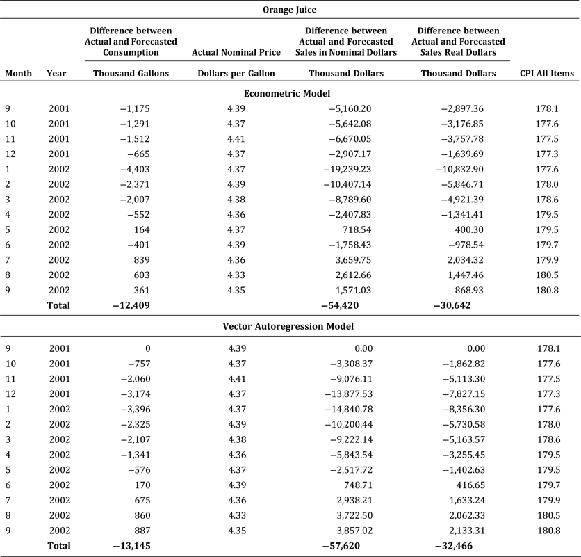
We use the results of the econometric and vector autoregression models to explore the repercussions of generic advertising of orange juice nearly going dark. We first forecast per capita consumption of orange juice for September 2001 through September 2002 with FDOC's generic advertising in place and then calculate the difference between actual and forecasted consumption to estimate foregone consumption (in gallons sold) and sales associated with the lack of generic advertising. Table 6 presents the results of this analysis.
Table 6. Calculations Associated with the Repercussions of Nearly Going Dark: Comparison of the Econometric and Vector Autoregression Models

We find that actual consumption and sales for September 2001 through April 2002 were lower than expected if regular FDOC advertising efforts had been maintained. Eventually, actual consumption and sales rebounded, reaching forecasted levels in July, August, and September of 2002 in response to FDOC efforts in calendar year 2002. Over the thirteen-month period, the total cumulative losses related to going nearly dark amounted to 12.41 million gallons of consumption and slightly more than $54 million in sales.
Repercussions of Nearly Going Dark in 2001—Vector Autoregression Analysis
From equation 7, the historical partition of the vector X at any date T + k can be divided into information available at time t = T and information revealed at period t = T + 1, T + 2, … , T + k. Specifically, the vector X at period T + k can be written as
 $${\bf X}_{T + k} = \sum\limits_{s = 0}^{k - 1} {\Theta _{s} v_{T + k - s} + \bigg[\sum\limits_{s = k}^\infty {\Theta _{s} v_{T + k - s} \bigg].}} $$
The position of the vector X that is due to information known up to period T is given by the term in brackets. Information revealed from T to T + k is given by the first summation expression on the righthand side of the equation. Each term (ΘsvT + k–s) is the product of a matrix (Θs) and the vector of innovations at period T + k – s (v T + k–s). For example, for k = 2, the representation of the moving average for per capita orange juice consumption can be written using the notation of the lowercase theta (θQOJ,FAD (0)), which denotes the element of the Θ matrix that corresponds to the row associated with the quantity of orange juice consumption per capita and the column associated with FDOC advertising expenditures at lag zero. The same holds for other variables and lags. Thus, the value of per capita consumption at period T + 2 can be expressed as a linear combination of historical innovations from each variable in the autoregression model as listed within brackets in equation 9.
 $$\eqalign{{X_{QOJ,T}}_{ + 2} & = {{\rm \theta }_{QOJ,QOJ}}\lpar 0 \rpar {v_{QOJ,T}}_{ + 2} + {{\rm \theta }_{QOJ,QOJ}}\lpar 1 \rpar {v_{QOJ,T}}_{ + 1} \cr & \quad \quad \quad \quad \quad \lsqb \hbox {per capita orange juice consumption} \rsqb \cr & \quad + {{\rm \theta }_{QOJ,POJ}}\lpar 0 \rpar {v_{POJ,T}}_{ + 2} + {{\rm \theta }_{QOJ,POJ}}\lpar 1 \rpar {v_{POJ,T}}_{ + 1} \quad \cr & \quad \quad \quad \quad \quad \lsqb \hbox {price of orange juice}\rsqb \cr & \quad + {{\rm \theta }_{QOJ,PGF}}\lpar 0 \rpar {v_{PGF,T}}_{ + 2} + {{\rm \theta }_{QOJ,PGF}}\lpar 1 \rpar {v_{PGF,T}}_{ + 1} \quad \cr & \quad \quad \quad \quad \quad \lsqb \hbox {price of grapefruit juice} \rsqb \cr & \quad + {{\rm \theta }_{QOJ,IN}}\lpar 0 \rpar {v_{IN,T}}_{ + 2} + {{\rm \theta }_{QOJ,IN}}\lpar 1 \rpar {v_{IN,T}}_{ + 1} \quad \cr & \quad \quad \quad \quad \quad \lsqb \hbox{ per capita income}\rsqb \cr & \quad + {{\rm \theta }_{QOJ,FAD}}\lpar 0 \rpar {v_{FAD,T}}_{ + 2} + {{\rm \theta }_{QOJ,FAD}}\lpar 1 \rpar {v_{FAD,T}}_{ + 1} \quad \cr & \quad \quad \quad \quad \quad \lsqb \hbox{ FDOC advertising expenditures on orange juice}\rsqb \cr & \quad + {{\rm \theta }_{QOJ,BAD}}\lpar 0 \rpar {v_{BAD,T}}_{ + 2} + {{\rm \theta }_{QOJ,BAD}}\lpar 1 \rpar {v_{BAD,T}}_{ + 1} \quad \cr & \quad \quad \quad \quad \quad \lsqb \hbox{branded advertising expenditures on orange juice}\rsqb \cr & \quad + {{\rm \theta }_{QOJ,OAD}}\lpar 0 \rpar {v_{OAD,T}}_{ + 2} + {{\rm \theta }_{QOJ,OAD}}\lpar 1 \rpar {v_{OAD,T}}_{ + 1} + bas{e_{QOJ,T}}\quad \cr & \quad \quad \quad \quad \quad \lsqb \hbox{advertising expenditures on other fruit juices}\rsqb }$$
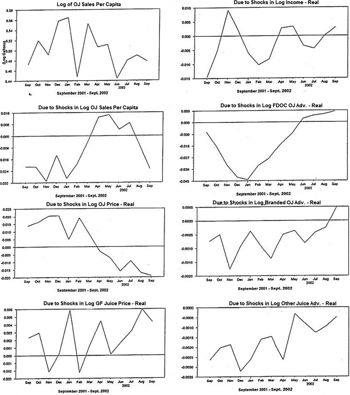
Figure 3 presents the historical decomposition of orange juice consumption based on information through August 2001 and the one-lag vector autoregression. Using the information known in August 2001, we forecast future months through September 2002. For each forecasted month, the difference between actual sales of orange juice and forecasted consumption can be expressed as effects arising from each of the seven variables included in the model. Each panel of Figure 3 shows the error made in forecasting orange juice sales based on information through August 2001 due to the actual realization of that particular series over subsequent months (September 2001, October 2001, November 2001, … , September 2002).

Figure 3. Historical Decompositions of the Logarithm of Orange Juice Sales per Capita
The uppermost lefthand panel in Figure 3 shows the logarithm of orange juice sales for September 2001 through September 2002. This actual series differs from the forecasted series (which was based on information known in August 2001) because of surprises (shocks) that actually occurred at each date in each of the seven series. These surprises (relative to what the series were thought to have been based on information through August 2001) contributed to the actual series as given in equation 9 by the amount plotted in each graph in Figure 3.
The shock effect of reduced advertising expenditures by FDOC is shown in the second righthand panel in Figure 3. The negative contributions of nearly going dark peak in January 2002 and get gradually weaker thereafter; in June 2002, actual consumption exceeded the predicted level. The panel shows lags associated with advertising expenditures and the subsequent response of sales, thus illustrating the “opportunity cost” of the near absence of advertising. As previously noted, FDOC made rather large advertising expenditures in the first six months of 2002. Those expenditures had a positive effect on orange juice consumption, but consumption did not fully rebound during that period.
Limitations
In our analysis, we highlight the ramifications of FDOC generic advertising nearly going dark with attention centered on impacts on consumer sales. We perform two quite different analyses using a structural econometric model and a vector autoregression model to examine the impact of the natural experiment presented by FDOC's actions. We hypothesized that the structural model consisted of a single quantity-dependent demand equation. A Hausman test revealed that the real price of orange juice was indeed exogenous so a single-equation specification was deemed appropriate. Therefore, we only addressed impacts on the quantity of retail sales in the marketing chain in the absence of a supply response. Taking the supply response appropriately into account would have required a multi-equation model to capture all of the agents in the marketing channel—orange growers, processers, and consumers. Measuring the impacts of advertising and promotion on all facets of the marketing chain exceeded the scope of the study.
The vector autoregression approach provided a multi-equation model that included per capita consumption of orange juice, the price of orange juice and grapefruit juice, disposable personal income, FDOC and branded advertising expenditures for orange juice, and advertising expenditures on fruit juices and drinks other than orange juice as endogenous variables. Consequently, we could consider a multi-equation specification to analyze the retail level of the marketing channel.
We did not include a demand system for the nonalcoholic beverage category because comparable data on grapefruit juice or other beverage products corresponding to the category were lacking. Therefore, the inter-relationships of nonalcoholic beverages are not captured, which may affect the magnitude of the impacts on consumer sales.
Concluding Comments
According to the estimation results from both the econometric (structural) and time-series (vector autoregression) models, the primary drivers of orange juice demand are the real price of orange juice, seasonality, and real FDOC expenditures for orange juice advertising. Additionally, the results from both methodological approaches agree that neither real per capita income nor real branded advertising expenditures on orange juice are statistically significant determinants of demand. The lack of significance of income as a driver of demand is at odds with Brown (Reference Brown1986), which estimated an income elasticity of 0.76. Our econometric analysis provides evidence that the real price of grapefruit juice and expenditures for advertising of other fruit juices are also key elements affecting orange juice demand. However, that conclusion is not supported by the time-series analysis.
Notably, the two approaches to analyzing repercussions of the lapse in FDOC's orange juice advertising in September, October, and November 2001 provide mutually supportive evidence of the opportunity cost of nearly going dark. The estimated cost in terms of lost orange juice consumption is 12.41 million gallons in the econometric analysis and 13.15 million gallons in the autoregression analysis. The estimated loss of sales revenue in nominal dollars is $54.4 million in the econometric analysis and $57.62 million in the autoregression analysis. Therefore, despite the limitations previously mentioned, the implication of our results is that even a short lapse in generic advertising can have a sizeable effect on consumption and sales revenue.
Our findings are similar to results reported by Crespi and Sexton (Reference Crespi, Sexton, Kaiser, Alston, Crespi and Sexton2005) in which the almond industry in California suffered substantially in terms of loss of profits due to the three-year suspension of the Almond Board's advertising program imposed by litigation; the study estimates range from $84 million to $231 million. The similarity of these results, which are both based on natural experiments that corresponded to counterfactual scenarios, points to the potential shortcomings of using theoretical counterfactuals to estimate the impacts of generic advertising.
Based on the vector autoregression analysis, a one-period lapse in generic advertising can affect demand well beyond the nearly-dark period. In the case of orange juice in the United States, a rebound in demand did not occur until eight or nine months after the lapse in advertising and six or seven months after advertising resumed. Thus, going dark for three months resulted in losses over a period two or three times longer than lapse.
The goal of generic advertising by commodity check-off groups is to create streams of revenue and therefore benefits to those who fund the advertising through a fee (check-off) on units they sell—primarily producers and sometimes others in the value chain. The highly variable nature of agricultural production year to year, both routinely and from less common events such as droughts and other natural causes experienced in the United States in recent years, leads inevitably to annual variability in the revenue received by check-off programs and thus in the availability of funds for generic advertising. The research presented here demonstrates that reductions in generic advertising are followed by losses that extend far beyond the period of little or no advertising. Whether the result of natural causes, legislative changes, internal decision-making, or legal challenges, a reduction in generic advertising is likely to result in a nontrivial opportunity cost for the associated commodity check-off organization.


