Profitability of Virginia's Agritourism Industry: A Regression Analysis

Abstract

Virginia's growing agritourism industry provides additional income to farms and mitigates risk. This study empirically analyzes the effect of demographic, operational, and financial factors on the profitability of agritourism operations using a primary data set collected from a survey of more than 500 agritourism operations. Results show that greater profitability is associated with operators who are motivated by additional income and have more education, larger operations with a greater percentage of income from agritourism, and visitors who spent more on average. Characteristics having a negative effect on profitability are wineries, locations farther from interstates, and difficulty accessing capital.

Agritourism is a value-added product that can generate additional income and introduce a farm brand to customers (Hawkes 2013). It also allows for diversification of income sources and decreases risks associated with market production and income. Tew and Barbieri (2010) suggested that diversification from purely production agriculture to production and agritourism is a low-risk mechanism farmers can use to cope with the rising cost of production inputs and technologies. Agritourism also can make it easier for farmers to weather bad crop years, disasters, and droughts (Hawkes 2013). Other economic and noneconomic benefits from agritourism include preservation of an agricultural heritage, maximization of productivity and resources, and improvements in the economy of the community (Tew and Barbieri 2012).

In the United States, agritourism has grown in popularity and, as a result, in economic importance. Demand for agritourism venues has been growing; according to Bernardo, Valentin, and Leatherman (2004), 62 percent of all U.S. adults in 2004 had visited a rural destination in the preceding three years. Furthermore, since 2002, income from agritourism nationwide more than doubled, generating an average of about $24,400 per farm for the 23,350 farms surveyed for the U.S. Department of Agriculture's (USDA's) 2007 Census of Agriculture (Hawkes 2013). The 2012 Census of Agriculture revealed an average farm income of $21,230 for 33,161 farms (National Agricultural Statistics Service (NASS) 2013a)—an increase in the number of agritourism operations and a decrease in their incomes, though the per-farm income still was greater than in 2002 despite the recession that took place between 2007 and 2012.

Despite the growing relevance of agritourism, empirical research on it remains underdeveloped and has focused mainly on motivations behind starting an agritourism operation. One important gap in the literature is financial analyses of the agritourism sector. With this in mind, we studied factors that contribute to the profitability of agritourism businesses in Virginia, including the demographic characteristics of operators and characteristics of the farms, for more than 500 agritourism operations in the state. For that analysis, we first developed a database of Virginia agritourism businesses that included more than 500 operations. We then conducted a survey that focused on assessment of the operations’ profitability following the Dillman method (Dillman, Smyth, and Christian 2014). In the empirical model, the dependent variable was the perceived profitability of respondents’ businesses rated on a 1–5 Likert scale. Because this variable was categorical, an ordered logit model was used to estimate the likelihood that an agritourism operation was profitable. The empirical results suggest that wineries, operations in which operators lack access to capital, and farms located relatively far from major transportation networks (interstate highways)¹ are less likely to be profitable. Variables associated with increased profitability are operators with a higher level of education, operators who were initially motivated by the potential for additional income, the number of acres, the percentage of gross income generated from agritourism, and the average amount of money spent by visitors. In summary, this study contributes to the agritourism literature by assessing the profitability of Virginia agritourism operations and identifying factors that affect their financial performance.

Literature Review

Agriculture is the largest industry in Virginia with an economic impact of about $52 billion and provision of more than 357,000 jobs (Virginia Department of Agriculture and Consumer Services (VDACS) 2013a). In addition, value-added industries that depend on farm products employ 76,000 individuals and generate another $34.6 billion in revenue (VDACS 2013a).

Despite the impact of the agriculture industry on Virginia's economy, some trends are concerning. First, small and medium sized farms have not been able to capture scale efficiencies due to resource constraints, and that inability has led many farmers to supplement their incomes. In this context, agritourism can be regarded as a feasible business venture that can decrease risk by supplementing and diversifying a farmer's income stream. According to Brown and Reeder (2007), agritourism can offset sudden changes in income associated with variation in weather, prices, and government payments. Furthermore, managers of small farms can position their businesses so that they can capitalize on ongoing increases in demand for locally sourced and sustainably produced agricultural products along with value-added products from their farms.

A second issue is the loss of 3,000 farms (6 percent) and 700,000 acres of farm land between 1998 and 2012 (NASS 2013a). An analysis of the size of such farms shows that the number of smallest farms (less than $2,500 in annual sales) and number of largest farms ($500,000 or more) have grown between 1997 and 2007 while the number of small and medium sized farms decreased (NASS 2013a). In addition, as shown in Table 1, the average age of farmers has been increasing, which could pose a threat to the sustainability of future agriculture operations. These constraints on land and human capital could potentially undermine the future of Virginia's agricultural industry, especially for small and medium sized operations.

Table 1. Virginia Farming Trends 1997–2012

Sources: NASS (2013a), VDACS (2013a, 2013b).

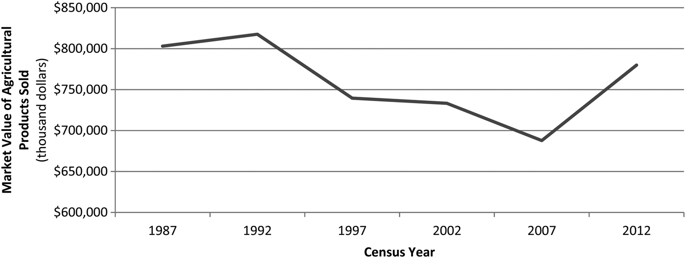
Along with the loss of farm land in Virginia, there has been a loss in the market value of agricultural production from the state (see Figure 1). Between 1992 and 2007 (pre-recession), the value of production from medium sized farms ($250,000 to $499,999) gradually declined. And while the market value of agricultural products sold by the smallest Virginia farms (less than $100,000) remained fairly constant from 1987 to 2007, the gross revenue of farms in the $100,000 to $500,000 range for annual sales mostly declined during that period. There was a modest rebound for the mid-range farms and a larger rebound for larger farms in 2012, after the economy improved. In contrast, the market value of products from the largest farms (sales of $500,000 or more) mostly increased. Consequently, operators of the largest farms may lack an economic incentive to add agritourism activities.

Source: NASS (2013a, 2013b).

Figure 1. Class Typology and the Market Value of Agricultural Products Sold in Virginia 1987–2007

Figure 1 also shows that incomes from farms with less than $100,000 in gross revenue have been relatively stable, which suggests that the significant decline in market value of products from the highest tier of small farms ($100,000 to $249,000) represents the overall topology of small farms in Virginia (see Figure 2). In addition, the revenue of mid-sized farms ($250,000 to $499,999) has gradually declined over the last 25 years. Consequently, Virginia's agricultural industry is arguably becoming bimodal—characterized mostly by small and large farms. According to Kirschenmann et al. (2008, p. 3), mid-sized farms are “too small to compete in the highly consolidated commodity markets and too large and commoditized to sell in the direct markets.” Overall, then, small and medium sized farms need to expand their incomes from on-farm and off-farm activities.

Source: NASS (2013a, 2013b).

Figure 2. Total Value of Agricultural Products Sold in Virginia for Small Farms 1987–2012

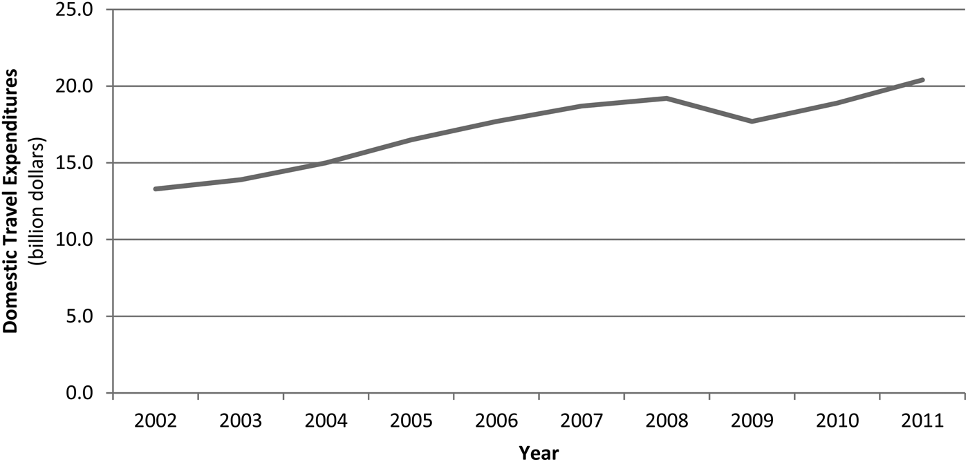
Virginia's tourism sector, on the other hand, has expanded and has had a positive effect on employment, incomes, and tax revenue, both directly and indirectly. According to electronic door counts at welcome centers in the state, there has been a steady increase in the number of visitors, growing from almost 1.4 million in 2007 to more than 2.3 million in 2012 (Virginia Tourism Corporation (VTC) 2013), a 64 percent increase.²Figure 3 shows that, with the exception of years surrounding the recent economic recession, there has been a steady increase in revenue from Virginia's tourism industry over the past decade. In 2012, the industry generated more than $21.2 billion for the commonwealth, a 4 percent increase over 2011. Tourism-related employment also increased, from 204,000 in 2010 to 210,000 in 2012 (VTC 2013), and tax revenue generated by tourism-related domestic travel in Virginia in 2012 reached $2.7 billion, a 3.3 percent increase over 2011 (VTC 2013). Thus, tourism has become increasingly important to Virginia's economy, and there is good reason for the state's agricultural industry to explore profitable ways to capitalize on agriculture-related tourism opportunities as part of an effort to offset recent economic losses.

Source: Virginia Tourism Corporation (2011).

Figure 3. Domestic Travel Expenditures in Virginia 2002–2011

Most recent analyses of agritourism have studied motivations behind the decision to start an operation (Brown and Reeder 2007, Nickerson, Black, and McCool 2001)³ and determined that the most common motive was generation of additional income or some other form of monetary incentive. Nickerson, Black, and McCool (2001) in a study of agritourism in Montana found that additional income ranked highest and was followed by more efficient use of resources and to assuage fluctuations in agricultural income, all of which are financial-based decisions. In a study of California agritourism (George et al. 2011), 75 percent of the respondents cited a need to increase profitability as a reason for entering into agritourism. Similar results were reported for the states of Virginia, Washington, and New Jersey and for Canada (McGehee and Kim 2004, Galinato et al. 2011, Schilling et al. 2006, Barbieri 2010). In summary, economic motivations, such as additional income or generation of profits, appear to be the main motivations for starting an agritourism venture.

According to Nickerson, Black, and McCool (2001), increasing financial strains on family farms had put pressure on those businesses to venture outside of traditional forms of agriculture to maintain their operations. A study by McGehee and Kim (2004) supported that view and cited a variety of reasons for the farmers’ desires to diversify: poor agricultural commodity prices, rising production costs, globalization, industrialization, encroachment by suburban development, loss of government-supported agriculture programs, and elasticity in commodities markets. Nickerson, Black, and McCool (2001) proposed two potential avenues for such farmers: (i) alter production and increase revenue or (ii) seek alternative sources of income to supplement the loss. The first is likely to be beyond the reach of operators of small farms due to land constraints that preclude them from expanding their operations. Agritourism, on the other hand, can increase and diversify returns on their investments through development of farm-based recreation (Brown and Reeder 2007). Tew and Barbieri (2012) found in a study in Missouri that the majority of respondents reported an increase in farm profit after adding an agritourism venture. The study also found that operators tended to profit more from sales of value-added items than from the agritourism activities themselves.

A prime illustration of how agritourism can support agriculture and rural communities is Virginia's wine industry and its notable growth. In 1979, Virginia had just six wineries. By 2007, there were 130 (VDACS 2013b), and by 2012 there were 250, a 75 percent increase from 2007 (Virginia Wine 2013). The economic impact of those wineries has been substantial; revenue from the wine industry almost doubled between 2005 and 2010, when it reached $750 million. The number of tourists associated with the wineries increased by 620,000 (Felberbaum 2012) and the number of jobs associated with the industry increased by nearly 1,600 (Virginia Wine 2013) over the same period. Wineries that are open to the public are considered agritourism operations since they offer tours, tastings, parties, and special events such as weddings. Thus, the recent increase in wineries in Virginia has provided an example of the potential for growth for other agritourism operations. Future synergies between the agricultural industry and an expanding tourism sector could provide additional revenue for farmers and create complementary sources of revenue for rural areas as exemplified by the wine industry.

Survey and Data

In terms of the mid-Atlantic and southern regions, several studies of agritourism have been conducted in surrounding states such as Tennessee (Jensen et al. 2006) and North Carolina (Xu and Rich 2014); however, they were limited to discussions of survey results and lacked an empirical analysis. The most recent study that focused on Virginia is McGehee and Kim (2004), which is likely outdated. The goal of this study is to provide updated information about Virginia's agritourism industry and to identify factors that have led to financial success. The first step is to define agritourism, which has not been formally defined nationwide. According to the Virginia General Assembly, an “agritourism activity” is

any activity carried out on a farm or ranch that allows members of the general public, for recreational, entertainment, or educational purposes, to view or enjoy rural activities, including farming, wineries, historical, cultural, harvest-your-own activities, or natural activities and attractions. Any activity is an agritourism activity whether or not the participant paid to participate in the activity. (Code of Virginia § 3.2-6400)

With this definition in mind, we developed a survey to obtain a detailed and more up-to-date picture of the outlook for agritourism operations in Virginia. The survey consisted of 33 questions presented in six sections: demographic attributes, characteristics of any agritourism operations, financial positioning, obstacles to success in the agritourism industry, contributors to success in the industry, and future plans and feedback. The demographic questions elicited gender, age, race, marital status, education, and experience with farming. The questions about the agritourism operation asked about the number of acres, seasonality, employees, and types of events offered. The contributors to success analyzed in the survey were use of promotion and advertising strategies and the farm's location. The section on future plans and feedback consisted of open-ended questions.

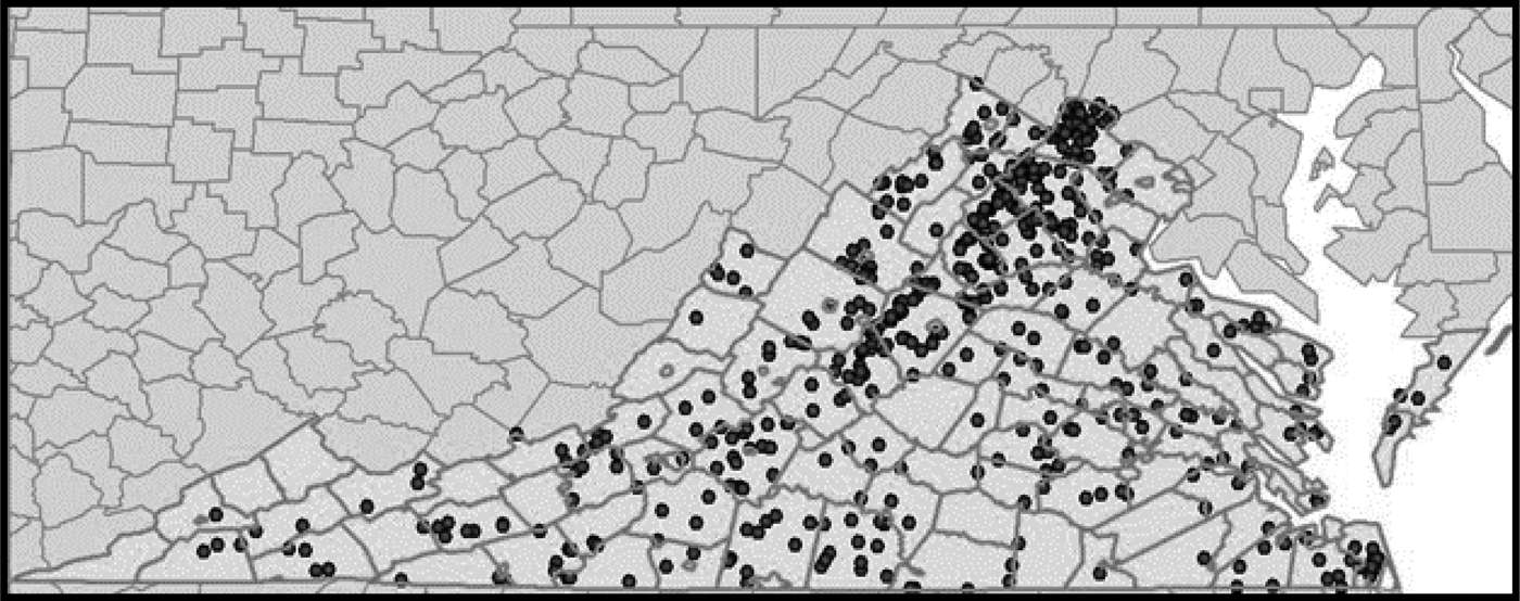
The study was based on a data set consisting of 511 agritourism enterprises in Virginia constructed using information from VDACS (2013a, 2013b), Virginia Wine (2013), Pickyourown.org (2013), and conversations with extension agents (see Figure 4). Forty enterprises were removed because they did not meet the research protocols,⁴ leaving a final data set of 471 operations.

Source: VDACS (2013a, 2013b), Virginia Wine (2013), Pickyourown.org (2013), extension agent correspondence, ArcMap 10.1.

Figure 4. Agritourism Operations in Virginia

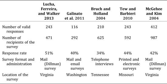
The survey was administered using a series of steps based on methods described by Dillman, Smyth, and Christian (2014)⁵ and generated 243 valid responses, a 52 percent response rate. The descriptive statistics of the data gathered from the survey are provided in an appendix that is available from the authors. Table 2 shows response rates for similar studies and the survey formats used in those studies; our response rate exceeded the rates for all of the studies listed.

Table 2. Comparison of Prior Surveys of Agritourism That Used Similar Methods

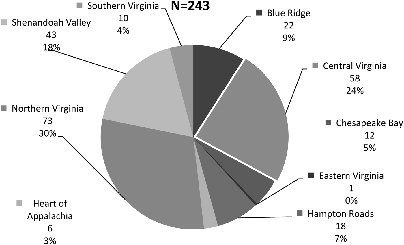
A temporal breakdown of the responses to our survey shows the diminishing response expected when using the Dillman method. The first mailing generated almost 59 percent of the total number of respondents, the second generated 25 percent, and the third generated 16 percent. A large portion of the respondents (44 percent) identified their operations as wineries. Figure 5 shows the percentage of respondents by region. The largest share, 30 percent, was from northern Virginia, which is located near a large population that has a high median income. Northern Virginia was followed by central Virginia at 24 percent and the Shenandoah Valley at 18 percent. The fewest respondents came from the eastern region (eastern shore). The lack of agritourism operations in that region is likely due to its limited number of population centers, lower median income, and lack of accessibility. Given the distribution of agritourism in 2013 (see Figure 4) and the fact that farmers are unlikely to establish agritourism enterprises in unprofitable regions, northern and central Virginia and the Shenandoah Valley are most likely to develop agritourism operations in the future.

Source: Lucha, Ferreira, and Walker (2013).

Figure 5. Breakdown of Respondents by Region

Empirical Model

First, the variables were analyzed to find each one's distribution and to adjust for scaling issues and other potential errors. An ordered logit is used in the empirical analysis because the dependent variable is a categorical that follows a sequential order in which the selection of level-2 profitability is better than the profitability of level 1, level-3 profitability is better than level-2 profitability, and so on.

Likert scales are often used to evaluate the qualitative type of data associated with this study. Tew and Barbieri (2010) evaluated the importance of accomplishing goals such as firm profitability on a five-point Likert scale, and other studies have evaluated motivations for starting agritourism ventures using a similar Likert-scale dependent variable (McGehee and Kim 2004, Galinato et al. 2011, Nickerson, Black, and McCool 2001, Tew and Barbieri 2012). In the survey, respondents were asked to evaluate the profitability of their agritourism ventures:

How would you rate the profitability of your agritourism operation or its contribution to the overall profitability of your farming operation on a scale from 1 to 5?

This question provided a discrete variable in which responses were ordered and mutually exclusive. An answer of 1 was coded as not at all profitable, a 3 as somewhat profitable, and a 5 as highly profitable.

According to Greene and Hensher (2010) and Badirwang (2012), the latent function is based on the following specification:

(1)$$y{^\ast} = {\bf \beta} {{\bf x}^{\prime}_i} + {{\rm \varepsilon} _i}\comma \; \quad i = 1\comma \; \, \ldots \, n$$

where y* is the unobserved dependent variable, i is the number of observations, x′;_i is a vector of independent or explanatory variables, β is the vector of coefficients associated with the independent variables, and ε_i is the error term. Following Badirwang (2012), and because there are five potential outcomes for the dependent variable Profit, the observed y _i is defined as

(2)$${y_i} = t\ {\rm if} \ {{\rm \theta} _t}_{-1} \le y{^\ast} \lt {{\rm \theta} _t}\, {\rm for}\, t = 1\comma \; \, 2\comma \; \, 3\comma \; \, 4\comma \; \, 5.$$

This general model can be transformed into five more-specific equations to describe each threshold parameter (Long and Freese 2006, Greene and Hensher 2010).⁶

(3)$${y_i} = \left\{\matrix{1\; {\rm if}\; {y^{\ast}} \lt {{\rm \theta} _1} \hfill \cr 2\; {\rm if}\; {{\rm \theta} _1} \le {y^{\ast}} \lt {{\rm \theta} _2} \hfill \cr 3\; {\rm if}\; {{\rm \theta} _2} \le {y^{\ast}} \lt {{\rm \theta} _3} \hfill \cr 4\; {\rm if}\; {{\rm \theta} _3} \le {y^{\ast}} \lt {{\rm \theta} _4} \hfill \cr 5\; {\rm if}\; {\theta _4} \le {y^{\ast}} \hfill} \right\}$$

This is a form of censoring, and the θs are unknown parameters to be estimated with β. Using equation 1 and substituting it into equation 2, we can specify the probability of observing one of the five categories of profitability as

(4)$$\eqalign{{\rm Pr}\lpar {y_i} = t \,\vert\, {x_i}\rpar &= {\rm Pr}\lpar {{\rm \theta} _{t - 1}} \le y{^\ast} \lt {{\rm \theta} _t}\rpar \cr &= {\rm Pr}\lpar {{\rm \theta} _{t - 1}} \le {\bf \beta} {{{\bf x}^{\prime}_i}} + {{\rm \varepsilon} _i} \lt {{\rm \theta} _t}\rpar .} $$

Simple mathematical transformation of the prior equation provides

(5)$${\rm Pr}\lpar {y_i} = t \,\vert\, {x_i}\rpar = {\rm Pr}\lpar {{\rm \theta} _t}_{ - 1} - {\bf \beta} {{\bf x}^{\prime}_i} \le {{\rm \varepsilon} _i} \le {{\rm \theta} _t} - {\bf \beta} {{\bf x}^{\prime}_i}\rpar \comma \; $$

and simple transformation results in

(6)$${\rm Pr}\lpar {y_i} = t \,\vert\, {x_i}\rpar = {\rm Pr}\lpar {{\rm \varepsilon} _i} \le {{\rm \theta} _t} - {\bf \beta} {{\bf x}^{\prime}_i}\rpar - {\rm Pr}\lpar {{\rm \varepsilon} _i} \le {{\rm \theta} _{t - 1}} - {\bf \beta x}^{\prime}_i\rpar .$$

Data Analysis and Model Development

The survey data are used in an ordered logit model to estimate maximum-likelihood parameters to identify factors that are most likely to be associated with profitability. For our application, the latent equation is

(7)$$\eqalign{Profit & = {\beta _1}lTimeIn{t_i} + {\beta _2}lCentral{2_i} + {\beta _3}North{7_i} + {\beta _4}East{345_i} \cr & \quad + {\beta _5}West{8_i} + {\beta _6}FarWest{16_i} + {\beta _7}Edu{c_i} + {\beta _8}Win{e_i} + {\beta _9}Even{t_i} \cr &\quad + {\beta _{10}}AgEx{p_i} + {\beta _{11}}AddIn{c_i} + {\beta _{12}}Hobb{y_i} + {\beta _{13}}DifAccCa{p_i} \cr & \quad + {\beta _{14}}lAcr{e_i} + {\beta _{15}}NatAme{n_i} + {\beta _{16}}Overnigh{t_i} + {\beta _{17}}ShareAgritou{r_i} \cr &\quad + {\beta _{18}}MsVisi{t_i} + {\beta _{19}}TotPro{m_i} + {\beta _{20}}CNA{S_i} + {\beta _{21}}Metr{o_i} \cr &\quad + {\beta _{22}}MetroCNA{S_i} + {\varepsilon _i}.} $$

The first variable, lTimeInt, accounts for the approximate time required to drive to the nearest interstate from the agritourism operation and is a measure of accessibility. lCentral2, North7, East345, West8, and FarWest16 are regional variables associated with the geographic location of each operation. Educ measures the education level of the primary operator. Wine and Event are variables for operational characteristics—whether the operation is a winery and the number of agritourism events offered at the farm. AgExp, AddInc, and Hobby assess the operator's experience in agriculture and motivations for starting the operation (as a hobby or for additional income). DifAccCap measures the degree of difficulty the operator has in accessing capital for the agritourism venture. lAcre represents the number of acres on which the venture operates, NatAmen represents the presence of natural amenities on the property, and Overnight designates operation of an overnight component. ShareAgritour represents the percentage of total income derived from agritourism, MsVisit denotes the average amount of money spent by each visitor, and TotProm represents the number of promotional channels the operator uses to advertise the business. CNAS represents the county's natural-amenity score (ERS 1999)⁷ and Metro is a variable calculated from the number of metropolitan areas near the operation and their respective populations. The last variable, MetroCNAS, is an interaction term for the two preceding variables to account for the effect of a geographic location that has a rural component and is accessible to consumers from more-urban areas. For a more detailed description of the variables in the empirical model, see the appendix, which is available from the authors.

Previous studies of the determinants of business success (Mary 2013) identified external and internal elements that affect performance. Thus, six hypotheses are used to test for links between various factors and the profitability of agritourism operations.

Hypothesis 1:

An agritourism operation located in northern Virginia is more likely to be profitable than agritourism operations in other regions of Virginia.

Northern Virginia offers a larger customer base, higher population density, and greater median income than other regions of the state. According to the U.S. Census Bureau (2013), Alexandria, Arlington, Falls Church, and Manassas Park have the highest population densities in the state among independent cities and counties with upwards of 5,000 people per square mile. In addition, Loudon, Fairfax, and Arlington were the top three counties in the United States in terms of income in 2011 (The Washington Post 2012). Clustering can also play a key role in the profitability of a region. Donaldson and Momsen (2011) argued that clustering can take on the role of networking among operations as well as allowing an easy flow of visitors from one agritourism operation to another. In this sense, northern Virginia is characterized by a high concentration of agritourism operations.

Hypothesis 2:

The operations farthest from an interstate are least likely to be profitable.

According to Sorupia (2005), modern transportation networks have created an ease and accessibility that have encouraged widespread growth of nature tourism in the United States. In terms of agritourism in particular, Jensen et al. (2006) found that easy transportation access was rated as extremely important or highly important by 71 percent of operators of Tennessee agritourism businesses who took part in a survey. Marrocu and Paci (2012) argued that a tourism destination that is easy to visit benefits from a greater inflow of tourists. Therefore, a variable that calculates driving time to the nearest interstate highway was included in the model as a proxy for ease of access and transportation costs.⁸

Hypothesis 3:

Operators who were motivated by additional income are more likely to be profitable than operators with all other motives.

It is reasonable to expect that operators who were motivated by income would focus on generating revenue and controlling costs by optimizing production and creating more-efficient methods.

Hypothesis 4:

Operations that have a more-diversified promotional portfolio are more likely to be profitable.

Promotional efforts lead to greater revenue streams. According to Sharma and Mehrotra (2007), multichannel promotion strategies can increase coverage by the firm, allowing it to reach a larger proportion of the customer base. Consequently, multichannel marketing strategies aid in consumer awareness and lead to enhanced sales and profits. Moreover, according to Bruch and Holland (2004), Tennessee operators identified advertising, marketing, and promotion as the most important factors in the success of an agritourism enterprise.

Hypothesis 5:

The presence of a greater number of natural amenities leads to a greater likelihood of being profitable.

Brown and Reeder (2007) cited two primary benefits of natural amenities: (i) providing consumers with more opportunities for recreation and (ii) enhancing the value of farm land. In addition, Bagi and Reeder (2012a) found that the percentage of U.S. farms involved in agritourism tended to be highest in areas that offered the most natural amenities, such as the Rocky Mountains. In general, tourism benefits from the presence of a certain natural element as tourists are attracted by the natural environment of a destination (Marrocu and Paci 2012). Therefore, the presence of natural amenities and recreation in a county could be important in defining a region's agritourism density due to the incentive those amenities provide to tourists.

Hypothesis 6:

Operations in proximity⁹ to relatively populated metropolitan areas are more likely to be profitable.

Relatively populated areas nearby provide a large supply of potential consumers. Bagi and Reeder (2012a), for example, found that distance to a city of at least 10,000 residents was negatively correlated with the probability of a farmer participating in agritourism. According to Bernardo, Valentin, and Leatherman (2004), the average distance a visitor in Kansas traveled to participate in on-farm activities was about 129 miles with 50 percent of the trips involving less than 50 miles. These results suggest that greater profits also come from this type of relatively easy access. Nasers (2009) found that 30 percent of Iowa State Fair attendees preferred to travel between 31 and 50 miles to an agritourism destination. In addition, Donaldson and Momsen (2011) found in a 2009 survey of agritourism in California that 50 percent of the state's 2.4 million visitors to agritourism venues came from within the county.

Before embarking on the empirical analysis, it is important to analyze the structure of the dependent variable because a Likert scale of profitability can be interpreted as a measure of perceived profitability rather than of actual profitability. To test the validity of the proxy in this study, the recorded answers on profitability were compared to other variables that were likely related to financial success: the average amount of money spent by visitors and the average number of visitors. These variables together represent the revenue generated by a farm's agritourism activities. The average money spent per visitor (median of each category (bin) for the variable denoting money spent per visitor) was averaged across profit levels.¹⁰ To estimate a median for the upper interval of money spent by visitors, $101 or more, an upper bound had to be designated.¹¹ Overall, this process revealed that the average amount of money spent per visitor increases as the agritourism operator's stated profit level increases, suggesting a monotonic link between average money spent per visitor and perceived profit (see Table 3). With the exception of outliers in profit level 3, the number of visitors also increases with perceived profit. These results provide further evidence for use of a perceived ordinal dependent variable (profit) since it is monotonically linked to more-concrete economic outcomes (money spent per visitor and number of visitors).

Table 3. Monotonic Links of Variables across Levels of Perceived Profit

Source: Authors’ calculations from the primary survey data.

A final argument for use of perceived profit over actual profit or some continuous function of revenue streams is the nature of the survey group. Farmers are typically reluctant to answer financial questions on surveys. According to Hoffman (1985), there is a need for data containing financial records of U.S. farmers because economic information and financial statistics are difficult to collect; however, it is difficult to collect financial data from farmers without running into nonsampling errors. Farmers may refuse to respond for a variety of reasons, including concerns about privacy and potential misuse of the data, not understanding the collection method, or lacking the time required to search for and provide the information (Thorpe 1985). Thus, asking for actual financial figures is likely to reduce the response rate.

Table 4 presents the distribution, which is symmetrical, and frequencies of the dependent variable. Most respondents (almost 48 percent) stated that they were profitable to some degree and selected a profit level of 3. Lower frequencies are found at the ends of the profitability spectrum; only 8.62 percent selected profit level 1 (not profitable at all) and more than 10 percent reported a large profit, selecting level 5. The distribution of the dependent variable was also analyzed by region and level of farm income generated by agritourism activities. Those results showed similar and stable distributions of the perceived profitability variable.

Table 4. Frequency of Perceived Profitability

Source: Authors’ calculations from the survey data.

Results and Discussion

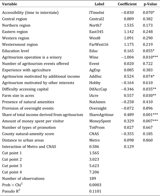
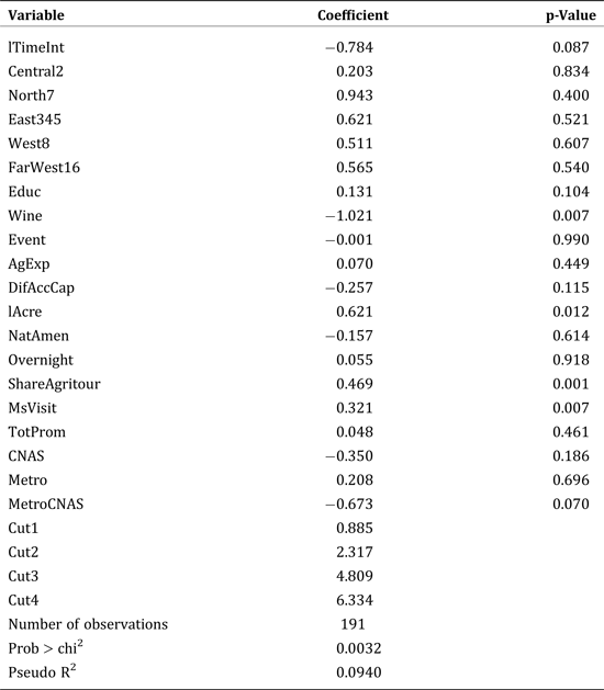
The ordered logit model (equation 8)¹² is estimated with White's robust standard errors, providing standard errors that are robust against heteroskedasticity and serial correlation and that partially correct for model misspecification (Long and Freese 2006). The results, which are presented in Table 5, are based on 189 observations¹³ and have a pseudo R² of 0.1101. The estimated p-value is 0.0003, which indicates that the model as a whole is statistically significant at the 1 percent level. A correlation matrix showed no multicollinearity issues between variables.

Table 5. Output of the Ordered Logit Model

Note: *** denotes a 1 percent significance level, ** denotes a 5 percent significance level, and * denotes a 10 percent significance level.

The estimation revealed no statistically significant difference in the profitability of agritourism operations in the southern region relative to operations elsewhere in the state so the southern region was used as the base level. This result contradicts hypotheses 1 and 6, which stated that operations located in northern Virginia and near large metropolitan areas were more likely to be profitable. This may be due, in part, to a lack of variation among the regions; the northern and central regions contain much of the state's population and supplied many of the observations. This is why some smaller groups (in terms of response rates) were combined into a single variable, which is signified by the number following the name of the variable.

The variable for time to the interstate (lTimeInt), a proxy for accessibility of an agritourism operation, shows the expected negative sign and is statistically significant. The longer it takes to reach the nearest interstate, the less likely an operation is to be profitable, which is in accordance with hypothesis 2. This is the only analysis made on the coefficient for an individual variable because coefficients in an ordered model do not tell us anything about the marginal effects of the variable on the probability of a certain outcome (Badirwang 2012).

The results also show that level of education of the operator is positively related to the operation's profitability. Being a winery has a significant and negative impact on profitability. This is particularly important since wineries account for nearly half of Virginia's agritourism operations. The lack of profitability may be explained by the fact that it takes about seven years from the day the vines are planted to generate returns from the vineyard and by the substantial initial capital investment required. As previously noted, the number of wineries in Virginia increased 75 percent between 2007 and 2013 (Virginia Wine 2013) so many of the state's wineries have been in business for less than ten years and are likely some years away from breaking even or making a profit.

The AddInc binary variable, which identifies additional income as an important motivation in starting an agritourism operation, has a positive and significant effect on profitably. This result confirms hypothesis 3 and supports the premise that operators who are motivated by money are also more focused on the financial management of their businesses and more attentive to the costs and revenue associated with their operations. Those who have greater difficulty in gaining access to capital are less likely to be profitable, perhaps because of the greater cost they incur when borrowing. However, there could be simultaneity between this variable and profitability in the sense that less profitable businesses are also less likely to have access to capital.

Firm size has been widely studied as an internal determinant of firm performance. However, the empirical findings are mixed, and evidence of links between firm size and performance remain inconclusive (Garcia-Fuentes, Ferreira, and Kennedy 2013). The results from this study indicate that large operations (by acres) are more likely to be profitable as the coefficient for the acreage variable is positive and statistically significant. This is likely explained by efficient use of larger tracts of land to generate revenue, the ability to accommodate a larger number of visitors, or economies of scale. To assess for the presence of economies of scale, the model was estimated with the square of the operation's acreage to determine if acreage that was increasing at an exponential rate changed or increased the significance. The resulting term was significant but not as significant as the one in the original model, suggesting that there is a threshold in the relationship of acres and profitability.

Results for the variable representing the percentage of annual gross farm income attributed to agritourism show that farms that obtain a greater share of income from agritourism are more likely to be profitable. This may point to payoffs associated with specialization in the agritourism activities on a farm. Wineries, for example, may be focused mostly on organizing events and tours because those activities can generate greater revenue than individual wine sales. On the other hand, operations at which customers spend relatively more during their visits are also more likely to be profitable. Thus, agritourism businesses should both increase the number of visitors to their premises and provide incentives for those visitors to spend. It is important to recognize a potential effect associated with wine expenditures in terms of the overall results. Expenditures at wineries typically involve higher dollar amounts than expenditures for other kinds of agritourism services and products.

Although not statistically significant, the variable for promotion activities shows the hypothesized positive sign. A larger number of observations might reveal a positive and significant relationship between a diverse promotional portfolio and profitability.

To analyze the estimated results from the logit model further, we calculate the marginal effects of each independent variable for each outcome using the average-marginal-effects method. According to Long and Freese (2006), the marginal change in the probability of occurrence of a specified outcome for the dependent variable is given by

(8)$$\displaystyle{{\partial \Pr {\rm \lpar }y\; = \; t\; {\rm \vert} \; x\rpar } \over {\partial {x_k}}} = \displaystyle{{\partial F\lpar {{\rm \theta} _t}\; - \; x\beta \rpar } \over {\partial {x_k}}} - \displaystyle{{\partial F\lpar {{\rm \theta} _{t - 1\; }} - \; x\beta \rpar } \over {\partial {x_k}}}.$$

This is the slope of the curve relating the independent variable x _k to Pr(y = m | x) when holding all other variables constant.

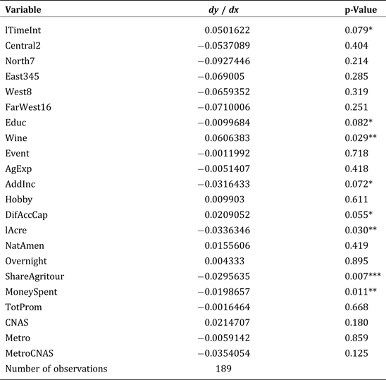
Table 6 reports the marginal effects of the independent variables for the predicted outcome of Profit = 1 (not profitable at all) using White's robust standard errors. The results show that the marginal effect of an operation going from non-winery to winery increases the likelihood of no perceived profitability by 0.06. When an agritourism operation increases the money spent by visitors by one category,¹⁴ the likelihood of no perceived profitability decreases by 0.02. For education, results suggest that a one-category increase in the operator's education level (from some college to a college degree, for example) decreases the likelihood of being at profit level 1 by 0.01. Other significant variables are the income motive and share of income from agritourism, which have negative signs. That is, a one-unit increase results in a reduction in the likelihood of the operation having no profit. For the accessibility variable (lTimeInt), there is a positive relationship with no perceived profit; a one-unit increase in the log of time to the nearest interstate increases the likelihood of being in the lowest level of profitability.

Table 6. Predicted Average Marginal Effects for No Profitability

Note: *** denotes a 1 percent significance level, ** denotes a 5 percent significance level, and * denotes a 10 percent significance level.

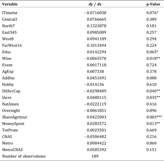
Table 7 shows the predicted average marginal effect of each variable on the probability of reporting profit level 5, very profitable, using White's robust standard errors. The sign of the winery variable changes, and the probability of an operation being very profitable is smaller when the venture is a winery. In addition, a one-level increase in the difficulty in accessing capital (from somewhat easy to somewhat difficult, for example) decreases the probability of being perceived as highly profitable by 0.03. Education, operation size, share of income from agritourism, and amount of money spent by visitors all have positive marginal effects; a one-category increase in each variable increases the likelihood of an operation being highly profitable. For the accessibility measure, a one-unit increase in time to the interstate leads to a decrease in the likelihood of the operation being highly profitability by 0.07.

Table 7. Predicted Average Marginal Effects for High Profitability

Note: *** denotes a 1 percent significance level, ** denotes a 5 percent significance level, and * denotes a 10 percent significance level.

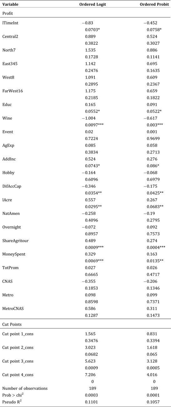
To further analyze the effect of these factors on profitability, an ordered probit model was estimated, and those coefficients and p-values are compared with the results of the ordered logit model in Table 8. There are no significant qualitative or quantitative differences between the two models’ outputs. It is important to note the difference between an ordered logit and a binary regression form of the logit model. An ordered logit reports cut points as threshold parameters while a logit model presents the cut point as a constant. The cut point is identical to the constant except that it has the opposite sign (Long and Freese 2006, Greene and Hensher 2010).

Table 8. Ordered Logit Model versus Ordered Probit Model

Note: *** denotes a 1 percent significance level, ** denotes a 5 percent significance level, and * denotes a 10 percent significance level.

A comparison of the results of the models reveals that the coefficients in the ordered logit point to larger impacts in most cases than the coefficients in the ordered probit. The ordered logit also has a slightly higher pseudo R² than the ordered probit. Furthermore, estimation of the Akaike and Bayesian information criterions shows that the ordered logit model has smaller values, making it a better fit.

The proportional odds assumption (also known as the parallel regression assumption) is an integral supposition in an ordered model. However, the assumption is often violated in the base specification of the model since it is common for the βs to differ across values of j (Williams 2006). According to Long and Freese (2006), the assumption states that βs are not allowed to differ across thresholds or cut points. For example, the coefficient that describes the lowest category against those higher is the same as the coefficients that describe the second lowest category and all higher categories. Based on equation 6, the probability that the dependent variable is equal to any of the outcomes is given by the following.

(9)$$\eqalign{& {\rm Pr}\lpar y \le 1 \,\vert\, x\rpar = F\lpar {{\rm \theta} _1} - {\rm \beta} {{x^{\prime}_j}}\rpar \cr & {\rm Pr}\lpar y \le 2 \,\vert\, x\rpar = F\lpar {{\rm \theta} _2} - {\rm \beta} {{x^{\prime}_j}}\rpar \cr & {\rm Pr}\lpar y \le 3 \,\vert\, x\rpar = F\lpar {{\rm \theta} _3} - {\rm \beta} {{x^{\prime}_j}}\rpar \cr & {\rm Pr}\lpar y \le 4 \,\vert\, x\rpar = F\lpar {{\rm \theta} _4} - {\rm \beta} {{x^{\prime}_j}}\rpar } $$

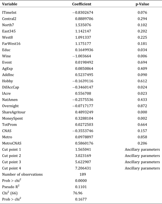
Thus, the coefficients are parallel because it is assumed that the β for each independent variable is equal for each equation. To test for the parallel regression assumption, an approximate likelihood-ratio test was performed. Those results are reported in Table 9. The null hypothesis posits that there is no difference in the coefficients of the models and that the parallel regression assumption holds (University of California Los Angeles (UCLA) 2014). The resulting p-value is 0.1677, and we therefore fail to reject the null hypothesis.

Table 9. Test of the Parallel Regression Assumption in the Ordered Logit Model

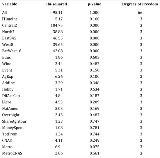
To test the parallel regression hypothesis for individual variables, the Wald test developed by Brant (1990) is used. A significant test statistic provides evidence that the parallel regression assumption has been violated. The results of this test are reported in Table 10. Again, the results show that the model as a whole does not violate the assumption of parallel regression. However, Wald tests for individual variables reveal some issues—the regional variables violate the assumption as their βs change depending on the outcome of the dependent variable. Despite these regional variables, the model as a whole rejects the fact that the assumption has been violated so a partial proportional odds model is not needed. For more on partial proportional odds models, see Williams (2006).

Table 10. Results of the Brant Test of the Parallel Regression Assumption

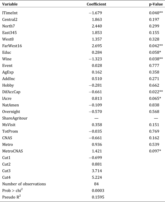
In a further investigation, we estimated the model using only operators who had indicated that 76–100 percent of their gross farm income was attributed to agritourism (ShareAgritour = 5). The objective of this regression was to test whether any of the factors are relatively more important to operators who invested heavily in their agritourism ventures. The results, which are presented in Table 11, suggest stronger relationships across the board; most of the significant variables from the original logit model became more significant. The largest difference from the original model is for the far western region, comprised of the Blue Ridge and Heart of Appalachia regions, which is now significant and positive. Because of the potential for lack of variance (there are only thirteen observations for the variable and eleven are from the Blue Ridge region), this result should be interpreted with caution.

Table 11. Results of Ordered Logit for Operators Who Obtained 76–100 Percent of Their Incomes from Agritourism

Note: *** denotes a 1 percent significance level, ** denotes a 5 percent significance level, and * denotes 10 percent significance level.

Another new finding is the significance of the interaction term for the natural amenities score and the normalized metropolitan area (MetroCNAS), which is positive. The significance of this coefficient suggests that these two factors reinforce each other. That is, operations located in an area that offers natural amenities and is near metropolitan centers are likely to be more profitable.

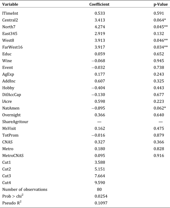
Table 12 shows estimates from the ordered logit model for operations in which agritourism accounted for less than 75 percent of income. Most of the regional variables are now significant. Thus, for operations in which agritourism is a relatively small contributor to income, the central, northern, western, and westerly-most regions all increase the likelihood of such operations being profitable relative to the base region (southern Virginia). In addition, the binary variable representing the presence of natural amenities is now significant and negative. When the agritourism operation accounts for a relatively small portion of the farm's income, a greater number of natural amenities on the property reduces the likelihood that the agritourism operation is profitable. Counties that have high natural-amenity scores may be more isolated geographically from major roads and metropolitan areas. In addition, perhaps additional visitors and related fees do not compensate for the cost to maintain the natural amenities and/or increased property values that result from their presence.

Table 12. Results of Ordered Logit for Operators Who Obtained Less than 50 Percent of Their Incomes from Agritourism

Notes: Operators reporting an agritourism share of level 1, 2, or 3. ShareAgritour = 4 is not included because at this level the share of agritourism revenue is still relatively high and the purpose was to capture those who had small-scale operations in terms of contribution to income. *** denotes a 1 percent significance level, ** denotes a 5 percent significance level, and * denotes a 10 percent significance level.

The estimates for operators who received a large share of their incomes from agritourism involved 84 observations. The p-value of the model is 0.0003 and the pseudo R² is 0.1595. The second model for all other operators involved 80 observations. In it, the p-value of 0.2753 is not significant and the pseudo R² is 0.1097. Despite the limitations of these models and their small sample sizes, the analysis sheds light on possible differences between farms that rely heavily on agritourism and those that do not.

Realizing the potential for endogeneity between the motivation factors (especially income) and profitability, we conducted one final test. Operators who are strongly motivated by income may also tend to work hardest to obtain a greater profit margin and to perceive themselves as more profitable. Thus, the variable for income as a motivation, AddInc,¹⁵ was dropped from the original model. Those results are presented in Table 13. Once again, the results are similar; there are only a few exceptions. The variables representing education level and difficulty accessing capital are no longer significant while the MetroCNAS interaction term is now insignificant and negative. Given the large body of literature on motivation factors in agritourism, it seems reasonable to focus on the original model that included income motivation as a factor in Virginia's agritourism sector.

Table 13. Results of Ordered Logit Model without the Motivation Variables

Note: *** denotes a 1 percent significance level, ** denotes a 5 percent significance level, and * denotes a 10 percent significance level.

The empirical results provide evidence that a series of factors influence the profitability of Virginia agritourism operations. The results do not support hypothesis 1; the regional variable for northern Virginia showed a positive sign but was not statistically significant in the original model. The negative and significant coefficient on the accessibility variable lTimeInt suggests that operations located farther from an interstate are less likely to be profitable, which confirms hypothesis 2. The empirical results also confirm the third hypothesis—operators who were motivated to start their agritourism operation by a desire for additional income are more likely to perceive their operations as profitable. The results fail to confirm the anticipated positive impact of a more diverse promotional portfolio on profitability (hypothesis 4). Further evaluation of individual methods of promotion¹⁶ may reveal more about the effectiveness of specific promotional strategies.

The fifth hypothesis posited that the presence of natural amenities on a farm has a positive impact on profitability. To evaluate the relationship between natural amenities and profitability, we used two variables: the number of natural amenities on the property (NatAmen) and the county's natural-amenity score (CNAS). In the original model, neither one was statistically significant, but in the model that included only operations with a large share of income from agritourism, the interaction term for the variables was significant. This indicates that an area that both offers natural amenities and is located near urban centers is likely to host relatively profitable agritourism businesses. It is important to note that the proxies for natural amenities have some limitations. Examples of such amenities were provided in the survey, but there could be some degree of subjectivity when operators responded regarding amenities on their properties. While the data on the natural-amenity scores (ERS 1999) may appear dated, it is reasonable to assume that natural amenities do not change significantly over time. The inconclusive results for hypothesis 5 justify further research.

The final hypothesis evaluated the impact of proximity to metropolitan areas on profitability. In the original model, the Metro variable was not statistically significant. In the analysis of operators who reported a large share of income from agritourism, this variable was interacted with the county natural-amenity score and the results were statistically significant. Thus, for operators who obtain a large part of their incomes from agritourism, a location that maintains natural amenities and is located near more densely populated metropolitan areas is important to the overall profitability of the operation. This result supports hypothesis 6 for some cases.

Conclusions and Policy Implications

Numerous factors could be associated with the recent growth of the agritourism industry in the United States, including a combination of lower agricultural commodity prices and rising production costs (a cost-price squeeze), globalization, industrialization, urban sprawl, loss of government programs that supported agricultural production, and elasticity in commodities markets (McGehee and Kim 2004). Tew and Barbieri (2012) attributed the growth to the fact that agritourism can increase a farm's revenue while serving other goals, such as enhancing quality of life. Agritourism may be a viable way to revive and restore mid-sized farms in Virginia, which have declined significantly in number since 1998.

Many studies have identified important drivers of agritourism development, but few have analyzed the profitability of this sector. To the best of our knowledge, this is the first empirical study of the effects of a series of factors on perceived profitability of agritourism operations. To complete the analysis, we developed a statewide survey of agritourism operators to collect data for the econometric analyses. Analysis of the data from the survey, which generated 243 valid responses and a 52 percent response rate, showed that almost 77 percent of the agritourism operators perceived their operations as profitable. The empirical analysis revealed several factors that affect the profitability of agritourism operations—farm size, accessibility by the public, access to capital, and the motivation for establishing the agritourism venue.

With respect to the optimal location, the results highlight the importance of the agritourism operation having ready access to transportation networks in the form of interstate highways. The other geographic conditions examined—proximity to urban areas, the region, and a greater number of natural amenities in the county—did not appear to impact profitability.

Specific features of the agritourism operation and some management practices are associated with profitability. Larger farms and operators who are especially focused on agritourism tend to be relatively profitable. Operators who are better educated and whose initial motivation for agritourism was to increase their incomes tend to be more profitable. At the management level, easier access to capital, obtaining a greater share of income from agritourism, and convincing visitors to spend more increases the likelihood of profitability. Wineries are found to be significantly less likely to be profitable than other types of agritourism operations. This is likely because most of Virginia's wineries were established less than ten years ago and so have yet to reap the benefits of their significant initial investments.

Perceived profitability provided a good proxy for actual profitability based on our robustness tests, but it has some limitations as well and the results should be interpreted with a degree of caution. In a study of 73 Iowa farms, for example, Duffy and Nanhou (2002) found that there were differences between perceived and actual profitability; some farm operators who perceived themselves as profitable were not. That study also found that prestige is important since the unsuccessful farms were larger than their counterparts were. Thus, bias can be introduced if operators of larger farms begin to associate the size of their operations or prestige with profitability.

Several policy recommendations can be drawn from the results of the empirical analysis. First, efforts to preserve natural amenities and their value must be balanced with increasing the accessibility of agritourism areas via transportation infrastructure. Second, state and/or local government authorities could develop programs to support wineries financially in terms of the initial fixed costs and lags in production. Finally, government and/or extension education programs could be developed for agritourism operators to improve their knowledge of business practices, management, agricultural practices, and other related fields. Those programs should address the need for certain economies of size and activity-focus in agritourism and the importance of improving their access to external financial resources. The latter could be achieved by increasing the quality of their accounting information, promoting the success of their products in the market, and demonstrating the viability of their business models (Amat and Elvira 2010).

Future research should further analyze the role of natural and constructed amenities. Bagi and Reeder (2012b) suggested a similar need for experimentation with “rurality” and its county-based demographic measures. Further analysis is also needed to accurately measure the profitability of agritourism operations, a task that will require information on the operations’ costs.