Evaporation from a cylindrical cavity: effect of gravity on the vapour cloud

Abstract

We examine the vapour cloud of a pure liquid evaporating from a millimetric cylindrical well/cavity/aperture. This is accomplished by injecting the liquid up a vertical pipe towards its outlet onto a horizontal substrate. The injection is halted before the liquid surpasses the substrate level. The resulting final state is a meniscus at or near the pipe's end. The analysis is realised by vapour interferometry (side view over the substrate) closely intertwined with simulations (including Stefan flow), which also help to fill up certain gaps in the measurements and provide computed evaporation rates. Comparison with experiment is facilitated by converting the computed vapour clouds into interferometric images, especially helpful when an inverse (Abel-type) conversion is difficult. Experiments are conducted in both microgravity (via parabolic flights) and ground conditions, thus enabling direct assessment of the role of gravity. The contrast is accentuated by a working liquid with heavy vapour (refrigerant HFE-7100), when instead of being flattened on ground the vapour cloud assumes a roughly hemispherical shape in microgravity. Furthermore, a non-trivial vapour-cloud response to the flight ${\rm g}$-jitter (residual gravity oscillations) is unveiled, ${\rm g}$-jitter vibrations posing a challenge for interferometry itself. A number of undesired but curious side issues are revealed. One concerns vapour formed deep inside the pipe during rapid injection and subsequently ejected into the field of view, which is detected experimentally and quantified in terms of vapour Taylor dispersion in the pipe. Others are an injection volume anomaly and parasitic postinjection specifically observed in microgravity conditions.

1. Introduction

In the majority of experimental studies concerning evaporation, the dynamics of the liquid phase alone are often emphasized, with limited attention given to direct measurements of the processes occurring in the gas phase. Nonetheless, a vapour cloud is a key imprint of the evaporation process. Its visualization contributes to a better understanding of the factors influencing the evaporation and, in particular, the evaporation rates. By employing the subtle science of digital vapour interferometry, the dynamics of the vapour cloud surrounding an evaporating surface can be assessed. The application of vapour interferometry for studying evaporating droplets and films has been successfully realised by a few researchers in the past (O'Brien & Saville 1987; Dehaeck, Rednikov & Colinet 2014; Braig et al. 2021). In the current study, we focus on quantifying the vapour cloud emitted from a localized evaporation site into an extended volume of ambient gas. Our particular interest lies in understanding the impact of gravity levels on the vapour cloud. To this purpose, we conduct experiments using a specially designed set-up both on ground and in the microgravity environment of a parabolic flight. Additionally we perform extensive modelling of the vapour cloud behaviour to complement and support the experimental analysis.

Under the auspices of the European Space Agency (ESA), several experiments exploring evaporation (as well as condensation and boiling) in microgravity have either been realized or are planned for the different near-future onboard platforms. As gravity is likely to mask specific physical mechanisms, weightlessness serves as a valuable tool to investigate them. The duration of microgravity ranges from a few seconds (drop tower) and tens of seconds (parabolic flights) to several minutes (sounding rocket) and months (International Space Station (ISS)). In particular, parabolic flights can serve as independent studies or be conducted as a part of the preparation or support for a space experiment planned for other space vehicles. Designing space host modules is a challenging task that often requires a rigorous preparatory testing phase and automatization.

The present parabolic flight experiment was intended to fulfil both these roles. Its conception aimed to test the essentials of vapour cloud measurement in a simplified set-up for use in space experiments involving evaporating sessile droplets (Kumar et al. 2020; Dehaeck et al. 2023). To this purpose, a reduced approach was followed as far as the localized vapour source is concerned: an evaporating meniscus inside a millimetric vertical pipe with an outlet onto a flat horizontal substrate was formed (stopping short of injecting a sessile droplet upon the substrate). At the same time, such a configuration forms a subject in itself, serving as a prototype for evaporation from millimetric wells and cavities (Shukla & Panigarhi 2020) and from the pipe's exit (Buffone, Sefiane & Christy 2017). Besides, such a configuration can also bear upon evaporation from micropores (Lu, Narayanan & Wang 2015), especially the microgravity part of the present study (gravity being negligible on the micropore scales). Furthermore, it represents an intermediate case between two more commonly studied scenarios. The first of them is the aforementioned case of sessile droplets (Popov 2005; Tsoumpas et al. 2015; Kumar et al. 2020; Dehaeck et al. 2023), while the menisci at the pipe's outlet can be regarded as an extension (to ‘negative heights’) within the family of sessile droplets. The other common scenario involves evaporation from a meniscus deep inside the pipe (Moosman & Homsy 1980; Wayner 1999; Morris 2003; Zhang & Nikolayev 2021). Even if this latter scenario is not studied in itself in the present paper, it can nevertheless be observed in the form of an unexpected vapour eruption into the field of view at the end of the injection.

The microgravity quality achieved in parabolic flights is not as high as in other microgravity platforms (approximately $10^{-2}$ of Earth's gravity level, potentially reaching $10^{-3}$ for brief periods as discussed later in this paper, whereas it can reach $10^{-5}$ or less on sounding rockets and the ISS (Pletser & Russomano 2020)). Notably, there is an appreciable ${\rm g}$-jitter present and its significance varies depending on the phenomenon studied. Exploring the significance of ${\rm g}$-jitter on vapour cloud shapes is one of the storylines followed in this paper. Additionally, this serves as an opportunity to examine the vapour cloud's response to such disturbances.

Simulations of evaporating menisci are supposed to play a special role in the present study. Apart from clarifying the physical aspects, they will also help to fill certain gaps in the measurements (such as diagnostics inside the pipe) and, in this regard, serve as a diagnostic tool. A novel way of comparison with experiment, although already tested by Dehaeck et al. (2023), is used, by converting the simulated concentration fields to phase images equivalent to those obtained from postprocessing the experimental ones. This conveniently enables an immediate active one-on-one comparison, considering that an inverse conversion (from interferometric images to the concentration field) is not always feasible for various reasons in the present experiment.

The set-up, interferometry and operational sequence are detailed in § 2. The evaporation model is described in § 3. The results of ground and flight tests and the corresponding simulations are analysed in § 4. The conclusions are drawn in § 5. Certain details like the material properties, an auxiliary consideration of the vapour formation in the pipe during the injection, and the challenging intricacies of interferometric postprocessing under vibrations caused by ${\rm g}$-jitter are given in the appendices.

2. Experiment

2.1. Set-up

The testing hardware consists of an experimental rig, control rack with touchscreen monitors, interface hardware systems and CPUs, as well as nitrogen (N$_2$) canisters. The experimental rig consists of a cylindrical test cell with four optical access ports (figure 1). Additional ports are provided for instrumentation and gas transport. A metallic pipe with 4 mm internal diameter and 80 mm in length is welded to the centre of a stainless-steel substrate (or platform). The bottom of the pipe is connected to a flexible polytetrafluoroethylene (PTFE) tube (3 mm internal diameter) through a metallic connector. The length of the flexible tube is roughly 130 mm. The other end of the flexible tube is connected to an electrically operated three-way valve which acts as the inlet port to allow the injected volume of liquid from the syringe pump. The same port also serves as an exit port during the evacuation of the test cell. The HFE-7100 (NOVEC 3M) fluid has been used as a working fluid in all the cases presented in this study.

Figure 1. Schematic of the experimental set-up and Mach–Zehnder interferometry: LS, laser source; BS, beam splitter; TC, test cell; CL, condensing lens; M, mirror; C, camera with optics.

A Mach–Zehnder interferometry set-up (Dehaeck et al. 2014) is employed to capture the vapour distribution in the vicinity of the pipe outlet located in the centre of the platform (figure 1). The (horizontal) field of view is focused just above the substrate with the outlet, as accessed through the optical windows. A stable and reliable laser source (Cobolt Samba $\lambda =532$ nm laser with fibre pigtailing and coherence length $>100$ m) has been used to obtain high-quality interferometric images through the camera optics. The light from the laser is directed into a flat mirror (M1) through a condenser lens (CL). The circular condensed beam from M1 is split into two equal beams by the beam splitter (BS1). One beam is allowed to enter the test cell through the mirror M1, and the other beam serves as the reference beam. Both beams are again recombined by the beamsplitter (BS2) and captured using a camera (make IDS) with optics. The mirrors M1 and M2 (Newport:625-RC4-M) are adjusted to get raw interferometric fringes of the required period and orientation (finite-fringe mode).

All the optics, test cell, electronic devices and instruments are mounted on a custom-made breadboard ($1600 \times 600$ mm$^2$). The entire set-up is enclosed inside a Zarges box, as shown in figure 2, to contain any possible HFE-7100 and optical leakages.

Figure 2. Three-dimensional representation of the present experimental set-up enclosed in a Zarges box: NDF, neutral density filter; PS, ports for thermocouples, pressure sensor and N$_2$ inlet; OA, optical access; other acronyms are as in figure 1.

2.2. Interferometric postprocessing

The raw interferometric images are postprocessed into the so-called phase-wrapped images that capture the spatial variation of the optical phase increment $\Delta \varphi$ (hereafter simply the phase). These variations are mainly due to the presence of the vapour relative to pure nitrogen at the same ambient pressure and temperature in the cell. This is related to the corresponding increment of the gas refractive index $\Delta n$ by

(2.1)\begin{equation} \Delta\varphi(t,y,z)= \frac{2{\rm \pi}}{\lambda} \int \Delta n(t,x,y,z) \,\mathrm{d}\kern 0.06em x \quad \mathrm{modulo}\ 2{\rm \pi}, \end{equation}

where the integration is realized along the optical path across the test cell parallel to the substrate; $x$, $y$ and $z$ are the Cartesian coordinates (cf. also figure 2); $t$ is the time. For any time $t$, the phase-wrapped image is actually a density plot of the phase $\Delta \varphi (t,y,z)$ modulo $2{\rm \pi}$, which thus consists of zones where the function value varies just between $0$ and $2{\rm \pi}$. The boundaries between the zones (hereafter referred to as ‘fringes’) are obviously isocontours of $\Delta \varphi (t,y,z)$.

The mentioned basic postprocessing consists of the following steps. The fast Fourier transform is applied to the raw images, the necessary frequencies containing the phase information are filtered using a window (also known as window Fourier filtering), centred, and an inverse fast Fourier transform is applied after a shift to finally yield a phase-wrapped field. This process is implemented using an in-house MATLAB code. For more details of the postprocessing procedure, readers can refer to the previous articles (Takeda, Ina & Kobayashi 1982; Kreis 1986; Dehaeck et al. 2014), although in the present context one aspect of it (reference images) is worth examining further and we shall come back to it shortly.

A quick postprocessing tool is in-built with the camera viewer. With this tool, it is possible to view the phase-wrapped images (preferably at a low-sampling frequency) during the tests. This allows us to visualize the vapour distribution on the ‘live-mode’ camera feed. The postprocessing of the entire dataset is realized upon the completion of the tests.

Postprocessing of the measured interferometric images of the vapour cloud also involves argument subtraction of the so-called reference image obtained in the absence of the cloud. The alignment of the mirrors (cf. figure 1) is most certainly affected by the gravity level in view of the presence of spring elements, whereas it is obviously desirable to have the same alignment for the reference and actual measurements. Therefore, for flight runs, we strive for taking the reference images when the microgravity phase, corresponding to the flight ‘parabola’, has already began (cf. § 2.3). The parabolas for which this did not happen (when the reference images without the vapour cloud were taken at a still appreciable gravity level) were excluded from further consideration, because no meaningful interferometric analysis turned out to be possible in those cases. Furthermore, an added difficulty is that the presence of a strong ${\rm g}$-jitter (cf. § 2.3) during the parabola renders such precautions not fully sufficient as the mirrors still undergo vibrations with consequences on their alignment. The intricacies of interferometric postprocessing in such conditions are discussed in Appendix C, which is better read in conjunction with the flight results presentation in § 4.3.

Further postprocessing could in principle be considered, such as phase unwrapping, i.e. getting rid of modulo $2{\rm \pi}$ in (2.1) and obtaining a full value of $\Delta \varphi$. Then applying the inverse Abel transform to the result would yield $\Delta n(t,r,z)$ under the assumption of its axial symmetry, where $r=(\sqrt {x^2+y^2})$ is the cylindrical radial coordinate. Then knowing (or independently measuring) the proportionality factor between $\Delta n$ and the vapour concentration, the underlying axisymmetric vapour concentration maps could experimentally be reconstructed (Dehaeck et al. 2014; Shukla & Panigarhi 2020). Yet such further steps are not pursued here as they are deemed to be either not feasible or unpractical within the present study on account of the following reasons. First, except for the very initial moments, the vapour cloud extends horizontally beyond the actual field of view, rendering such a full reconstruction problematic. Second, the axial symmetry quality is somewhat compromised for the flight runs due to ${\rm g}$-jitter. Third, the fringes in the phase-wrapped images already provide a convenient and adequate visualization of the vapour cloud shape, as we shall see. Fourth, as far as comparison between experiment and theory is concerned, it can readily be carried out in terms of the phase-wrapped images. Indeed, in numerical simulations, the phase-wrapped field is readily obtained from (2.1) once the vapour concentration field has been computed (knowing the earlier mentioned proportionality factor).

2.3. Operational sequences in flight and on ground

A typical experimental flight sequence consists mainly of two alternating phases, as shown in figure 3: the test phase (T) and the preparation phase (P). The test phase corresponds to the parabola of the flight when the actual microgravity experiment test is performed. The ‘$g$’ (gravity level) data along the three directions is obtained from a triaxial accelerometer (make MEGGITT) positioned close to the experimental cell (cf. figure 3 for the typical course of the $z$ component). The total period and the gravity value during the parabolic flight manoeuvres depend on parameters such as the flight altitude, meteorological conditions, and sometimes even the pilot's experience and timings. During the microgravity phase, there is always a residual acceleration known as g-jitter, which disturbs the symmetry and may have a significant effect on the vapour cloud as we eventually find out in the present study.

Figure 3. A typical pressure and gravity-level cycle during the flight. The microgravity experiment run corresponds to the test phase T, which alternates with the preparation phase P. The operation timeline (OTL) with the steps 1–8 is described in the text.

Let us define the gravity vector $\boldsymbol {g}$ and its components $g_x$, $g_y$ and $g_z$ as

(2.2a,b)\begin{equation} \boldsymbol{g}=g_x \boldsymbol{e}_x+g_y \boldsymbol{e}_y-g_z \boldsymbol{e}_z,\quad \hat{\boldsymbol{g}}\equiv \frac{\boldsymbol{g}}{g_*}=\hat{g}_x \boldsymbol{e}_x+\hat{g}_y \boldsymbol{e}_y-\hat{g}_z \boldsymbol{e}_z, \end{equation}

where in view of certain convenience and conventions the $z$ axis is directed ‘upwards’ (cf. figure 2) whereas the $z$-component is defined as positive when directed ‘downwards’. The hat denotes the values normalized to the ground gravity level $g_*=9.81$ m s$^{-2}$.

The OTL in figure 3 details the intermediate steps during the two phases. All the operations, controls and data saving have been automated and can be executed just by pressing a digital button, as required in parabolic flight campaigns. The preparatory phase starts with filling the test cell with nitrogen to evacuate the residual liquid and the vapour from the previous test. The nitrogen (N$_{2}$) is supplied from an external gas bottle. The operation is indicated as step 1 in the OTL (filled green circle indicating the opening of the valve). An electrically operated, normally closed, two-way valve controls nitrogen flow into the cell. A pressure sensor (TERPS 8000 series, make GE) continuously monitors and records the pressure inside the cell. The pressure cycle of a typical parabolic manoeuvre is also presented in figure 3. The test cell is filled with N$_{2}$ up to approximately 1040 mbar, and the two-way valve is shut off, indicated as step 2 in the OTL (filled red circle indicating the shutting of the valve). In step 3, the three-way valve connected to the PTFE tube is opened to flush out the residual liquid in the pipe that is left over from the previous experiment along with the residual HFE-7100 vapour and $\mathrm {N}_{2}$ into a liquid trap. The three-way valve remains open to the liquid trap until the cabin pressure of approximately 860 mbar is recovered inside the cell. The flushing of liquid and gas mainly occurs when the flight is levelled at 1 g; however, before entering the next subsequent test (microgravity) phase, the gravity level attains a value of approximately 1.8 g. As any physical movement of the experimentalists during hypergravity (1.8 g) is not recommended due to motion sickness, the steps for the initiation of the test phase already start just before the hypergravity, as indicated in step 4 of the OTL. Though step 4 is initiated (by pressing a digital button), the sequence does not start right away. Instead, programming ensures that the exit port of the three-way valve first closes (step 5), and then the actual injection sequence is triggered (step 6) ideally a few seconds after the start of microgravity (as required for taking the right reference images, cf. § 2.2). This is quite challenging as the exact timing of the hypergravity phase is not the same for each parabola. Therefore, only specific cases where the injection sequences happened to be correctly initiated have been considered for our analysis.

The test phase consists of the injection stage (steps 6 to 7) and the evaporation stage (steps 7 to 8). During the injection stage, a predefined volume ($V_{inj}$) of HFE-7100 is injected into the pipe through the inlet port of the three-way valve at a given flow rate ($J_{inj}$) and an injection time ($t_{inj}=V_{inj}/J_{inj}$). During these stages, all necessary data, such as pressure, temperature and gravity level, are stored along with the vapour cloud evolution captured through interferometry. Several thermocouples have been fixed to the platform and the internal walls of the test cell to monitor the substrate and the gas temperatures. Finally, after another passage through 1.8 g, the test phase is ended by returning to 1 g conditions (step 1). This operational sequence is repeated for each parabola.

On ground, this sequence is similar, except that the internal test cell pressure is maintained at an ambient pressure of 1013 mbar (instead of 860 mbar during the flight) and the gravity level is normal (1 g). Also, the cell pressure is increased up to 1200 mbar during the preparation phase, after which the cell is flushed until the ambient pressure is reached.

Experiments were initially performed in ground conditions (1 g), and the liquid injection volume necessary to position the meniscus close to the outlet of the pipe was estimated to be $V_{inj}=1.95$ ml (the injection rate used being $J_{inj}=0.5$ ml s$^{-1}$). The position of the meniscus was confirmed visually by opening the top cover of the cell for a trial test case. However, during microgravity conditions, when the same volume was injected (although at a higher injection rate of $J_{inj}=1$ ml s$^{-1}$ to make the most of a limited time of microgravity), the liquid overflowed out of the pipe outlet, wetting the platform. Therefore, it was necessary to find the right injection volume whilst already in flight. To our surprise, in microgravity, $V_{inj}=1.60$ ml already turned out to be sufficient to ensure a meniscus position at the pipe outlet (without overflow). This is appreciably less (by 17 %) than the value precalibrated on ground. This newly calibrated injection volume turned out to be quite reproducible for at least three consecutive parabolas, manifesting a systematic character of the phenomenon. Our conjecture is that such a notable volume anomaly is related to gas trapping in the injection systems, which seems to occur only in microgravity. This could be the subject of a separate study, with a significance well beyond the present set-up. A similar volume anomaly (although in a weaker form than here) was arguably observed in sounding rocket experiments, when the injected sessile droplets turned out to be larger than intended and precalibrated on ground (Kumar et al. 2020).

For this injection volume recalibration in flight, the only observation method at our disposal were the live-mode phased-wrapped images (although at a quality appreciably inferior to any images shown in the present paper). For instance, when the injection volume exceeds the limit, the liquid overflows out of the opening onto the platform. This leads to the formation of a sessile droplet-like puddle (highlighted zone) as shown in figure 4(a), which is also understandably accompanied by a large number of fringes (large amount of vapour). Then the decision was to slightly lower the position of the meniscus. The injection volume was systematically reduced by small steps until no overflow was observed. This resulted in the observation of fewer fringes (figure 4b). Inversely, when the meniscus position was too deep (below 2 mm, as confirmed from ground experiments), the vapour concentration in the vicinity of the pipe opening was too low to produce any noticeable changes in the refractive index, resulting in no visible fringes. In that case, the injection volume was slightly increased until two to three fringes were visible. Hereby, we must note that there was no possibility of visually verifying the meniscus position in flight conditions as already mentioned. In this way, we are reasonably sure that the meniscus is eventually located at the opening (either pinned or slightly below, cf. figure 5 with further explanations later on). However, its precise position remained unmeasured and will be regarded as a fitting parameter when comparing the experiment with simulations.

Figure 4. Phase-wrapped images for the case where the liquid overflow creates a large number of fringes: (a) $V_{inj}=1.62$ ml. Typical images when there is no overflow for comparison: (b) $V_{inj}\approx 1.6$ ml.

Figure 5. Meniscus configurations used in simulations, cf. (3.8).

3. Theory

3.1. Basic assumptions, equations and boundary conditions

We now turn to the mathematical formulation used in the present simulations of the vapour cloud from an evaporating meniscus. The gravity acceleration $\boldsymbol {g}$ is therein set equal to either zero ($\boldsymbol {g}=0$) or the measured $z$-component of the ${\rm g}$-jitter as a function of time, $\boldsymbol {g}=-g_z(t)\boldsymbol {e}_z$, cf. also (2.2). An example of such a ${\rm g}$-jitter can be found in figure 3. Here, we limit ourselves to an axisymmetric formulation and hence discard the $x$- and $y$-components of the ${\rm g}$-jitter. When simulating for the ground runs, we have $\boldsymbol {g}=-g_* \boldsymbol {e}_z$ (where $g_*\equiv 9.81$ m s$^{-2}$), directed downwards orthogonally to the substrate.

The gas density $\rho _g$ varies by the order of itself throughout the vapour cloud. This is due to HFE-7100 being rather volatile (saturation pressure $p_{sat}\sim 0.2$ bar here) and having a relatively high molar mass relative to ambient nitrogen ($M_{HFE}\gg M_{N2}$). Hence, we cannot make the Boussinesq approximation. However, we still remain in the usual framework of an incompressible flow, in the sense that $\rho _g$ is not affected by hydrodynamic and hydrostatic pressure variations, which are much smaller than the ambient pressure $p_{amb}$. Furthermore, for simplicity, we shall here rely upon an isothermal model, disregarding evaporative cooling. The temperature is simply an input parameter (ambient temperature $T_{amb}$) and not a dependent variable. Thus, $\rho _g=\rho _g(\chi )$ is taken as a function of the vapour molar fraction $\chi$ at given $T_{amb}$ and $p_{amb}$. In contrast with $\rho _g$, the gas molar density $n_g$ is constant (under those assumptions and the ideal-gas assumption). The gas dynamic viscosity $\mu _g$ is defined as $\mu _g=\mu _g(\chi )$, similarly to $\rho _g$. The vapour diffusion coefficient $D_g$, following Bird, Steward & Lightfoot (2006), is assumed constant as well (depending on $T_{amb}$ and $p_{amb}$); cf. table 1 and Appendix A for further details on these and other properties.

Table 1. Basic properties (cf. Appendix A for additional details).

The Navier–Stokes equations in the gas (continuity and momentum) are then written as

(3.1)$$\begin{gather} \partial_t \rho_g + \boldsymbol{\nabla}\boldsymbol{\cdot}(\rho_g\boldsymbol{v}_g)= 0, \end{gather}$$

(3.2)$$\begin{gather}\rho_g (\partial_t\boldsymbol{v}_g + \boldsymbol{v}_g\boldsymbol{\cdot} \boldsymbol{\nabla}\boldsymbol{v}_g) =-\boldsymbol{\nabla} p_g + \boldsymbol{\nabla}\boldsymbol{\cdot} (\mu_g (\boldsymbol{\nabla}\boldsymbol{v}_g+\boldsymbol{\nabla}\boldsymbol{v}_g^T-\tfrac{2}{3}\boldsymbol{\mathsf{I}} \,\boldsymbol{\nabla}\boldsymbol{\cdot}\boldsymbol{v}_g) ) + \rho_g\boldsymbol{g}, \end{gather}$$

where $\boldsymbol {v}_g$ is the gas velocity field, $p_g$ is the hydrodynamic gas pressure (defined up to a constant) and $\boldsymbol{\mathsf{I}}$ is the unit tensor. As already mentioned, we have an incompressible flow in the sense that $\rho _g$ is not affected by $p_g$ ($\rho _g\neq \text {const.}$ being entirely due to the vapour field $\chi$). As a consequence, in spite of $\boldsymbol {\nabla }\boldsymbol {\cdot }\boldsymbol {v}_g\neq 0$, the bulk viscosity is immaterial and is not accounted for in (3.2) because the corresponding gradient term would merely amount to a redefinition of the hydrodynamic pressure $p_g$ without affecting the flow field.

The vapour molar fraction $\chi$ is governed by an advection–diffusion equation:

(3.3)\begin{equation} \partial_t\chi+\left(\boldsymbol{v}_g + D_g \frac{M_{HFE}-M_{N2}}{M_{HFE}\chi+M_{N2} (1-\chi)} \boldsymbol{\nabla}\chi\right) \boldsymbol{\cdot}\boldsymbol{\nabla}\chi= D_g \nabla^2\chi, \end{equation}

where the advection is realized by means of a so-called molar-averaged velocity (the term in parentheses on the left-hand side (Bird et al. 2006)). The form (3.3) is convenient when $\rho _g$ is greatly variable while the molar density $n_g$ is constant (as is here the case).

The boundary conditions include no slip and impermeability

(3.4)\begin{equation} \boldsymbol{v}_g=0,\quad \partial_n\chi=0 \quad \mathrm{at\ solid\ surfaces}. \end{equation}

On the other hand,

(3.5)\begin{equation} v_{g,n}=\frac{j}{\rho_g},\quad v_{g,\tau}=0,\quad \chi=\chi_{sat} \quad \mathrm{at\ the\ meniscus\ surface}, \end{equation}

where $\chi _{sat}$ is the saturation molar fraction,

(3.6)\begin{equation} j=-\frac{n_g M_{HFE} D_g}{1-\chi}\, \partial_n\chi \quad \mathrm{at\ the\ meniscus\ surface} \end{equation}

is the evaporation flux density [kg m$^{-2}$ s$^{-1}$], the denominator different from unity accounting for Stefan flow, $\boldsymbol {n}$ is the normal pointing to the gas, the subscripts ‘$n$’ and ‘$\tau$’ denote the normal and tangential components, respectively. According to (3.5), the normal velocity of the gas is due to evaporation; the tangential velocity is set equal to zero disregarding flow in the liquid relative to the one in the gas (in particular, disregarding a possible Marangoni convection, which is consistent with the present isothermal model). With (3.6), the evaporation rate $J_{evap}$ [kg s$^{-1}$] is obtained by integrating over the meniscus surface area:

(3.7a,b)\begin{equation} J_{evap}=\iint j\,\mathrm{d}S, \quad J_{evap}^*=\frac{J_{evap}}{\rho_{sat} D_g R}, \end{equation}

where a normalized evaporation rate $J_{evap}^*$ is also introduced with the scale given by the denominator, $\rho _{sat}$ being the saturation density. Note also that to express $J_{evap}$ in $\mathrm {\mu }$l s$^{-1}$ (as often used in the literature), one should multiply $J_{evap}^*$ by the scale provided in table 1.

Although we know that the meniscus is located inside the (circular) pipe close to the opening, its exact position and shape remain unmeasured. In view of this, when attempting a comparison between the experiment and simulations later on, those will just be treated as fitting parameters. Given such a level of detail, we limit ourselves to two particularly simple meniscus shapes in the simulations, which is deemed sufficient to capture the essence of the observed vapour clouds. Namely, we just consider spherical caps as well as flat menisci located at a certain depth, i.e.

(3.8)\begin{equation} h(r)=\left\{\begin{array}{@{}l} \sqrt{\dfrac{(R^2+h_a^2)^2}{4 h_a^2} -r^2} - \dfrac{R^2-h_a^2}{2 h_a} \quad (h_a\le R) \\ \sqrt{R^2 -r^2} + h_a-R \quad (h_a\ge R) \end{array} \right. \quad\text{and} \quad h(r)=h_a, \end{equation}

respectively, where $r\le R$, cf. figure 5. Here $r$ is the cylindrical radial coordinate, $h$ the local gas depth in the pipe (from the substrate to the meniscus surface) and $h_a$ is the depth along the symmetry axis. The latter will serve as the mentioned fitting parameter. In (3.8a), we consider at first (when $h_a< R$) spherical caps pinned at the edge of the opening. At $h_a=R$, the spherical cap becomes a hemisphere, and for $h_a>R$ we just consider hemispheres depinned from the opening and shifted down by $(h_a-R)$. Furthermore, we shall assume the meniscus shape unchanged during the evaporation, thus disregarding its possible receding for the time period of vapour cloud measurements. All simulations here are two-dimensional (2-D) axisymmetric.

3.2. Two kinds of simulations: benchmark quasisteady and real-set-up transient. Phase images

The simulations are carried out using the COMSOL Multiphysics software. Two kinds of simulations are realized in the present paper:

1. (i) Benchmark simulations. These are simulations in a somewhat reduced, more ‘standard’ arrangement representing the essence of the problem. Here, given that the evaporation cell dimensions are much greater than the pipe opening size, we disengage ourselves from the real cell geometry and rather resort to asymptotic boundary conditions $\boldsymbol {v}\to 0$ and $\chi \to 0$ far away from the pipe opening (formally at infinity, the gas phase thus occupying the half-space above the meniscus and the otherwise flat substrate, cf. figure 6). Furthermore, we just solve a (quasi)steady problem, with $\partial _t\equiv 0$ in (3.1)–(3.3). This is of relevance in the present context given that the typical diffusion time is ${\sim }R^2/D_g<1\ \mathrm {s}$. One of the goals is to represent in a concise and systematic way the typical vapour cloud distributions and evaporation rates as functions of the meniscus geometry (depth) and gravity level. Note, though, that such benchmark steady simulations are generally of limited utility as far as reduction to phase images is concerned, in terms of which, as earlier mentioned, comparison with experiment will be carried out. The matter is that the integral in (2.1) may not be converging for steady concentration fields $\chi (r,z)$ in a domain of a formally infinite extent ($\chi \to 0$ not sufficiently fast at infinity), where $\chi (r,z)$ gives rise to $\Delta n(r,z)$ through a proportionality factor provided in table 1. Thus, for phase images, we need to resort to the real-set-up transient simulations, where this impediment is remedied both by an eventually faster decay of $\chi$ in the transient case and by a finite domain considered (be it even large). Moreover, this will also be suitable for the initial stage, and not only for the already established vapour clouds.

2. (ii) Real-set-up simulations. These are transient simulations in a configuration as close to the experiment as possible. In particular, we adhere to the real (axisymmetric) geometry of the evaporation cell, as schematized in figure 7. Boundary conditions (3.4) are then used at all walls (not only at the substrate). Note that this corresponds, in fact, to a hermetically sealed cell, while a slight evaporation-related pressure increase is disregarded in the simulations, which can be justified by a large cell size and a limited time of observation. It is such real-set-up simulations that are used for a direct comparison with the experiment in terms of the wrapped-phase images. To this purpose, the computed axisymmetric vapour concentration field $\chi (t,r,z)$ is converted to $\Delta n(t,r,z)$ by means of table 1 and then used in (2.1) to compute $\Delta \varphi (t,y,z)$ (modulo $2{\rm \pi}$).

Figure 6. Geometry used in benchmark simulations. Asymptotic boundary conditions are imposed far away from the meniscus (symbolised by the dashed contour). The meniscus is represented just schematically (for shapes used in simulations rather cf. figure 5).

Figure 7. Basic evaporation cell geometry (axisymmetric, not drawn to scale), used in the real-set-up simulations. The gas phase, for which the simulations are carried out, occupies the space beyond the pedestal and the liquid column in the pipe. The meniscus is represented schematically (for shapes used in simulations rather cf. figure 5).

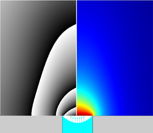
An important point for our analysis, already underscored in § 2.2, is illustrated in figure 8. It shows the typical phase-wrapped images alongside the underlying axisymmetric vapour concentration fields obtained in simulations for a flight parabola. Here we can see that the shape of our (heavy) vapour cloud in response to the flight ${\rm g}$-jitter (elongation along the axis for $g_z<0$ and flattening for $g_z>0$) is well representable by the fringes, even if they do not coincide with the isoconcentration lines. More detailed results will be provided in due course in § 4.

Figure 8. Typical phase-wrapped images together with the corresponding vapour concentration map for simulations in flight conditions.

While the problem formulation provided in § 3.1 is complete for the benchmark quasisteady simulations, it still needs to be complemented by the initial conditions for the real-set-up transient simulations. In experiments, a rather non-negligible amount of vapour is observed to be ejected from the opening into the field of view already during the injection. This still happens before the meniscus reaches its topmost position and the injection stops (the moment at which the formulation of § 3.1 is implied to enter into effect). Therefore, an appropriate initial condition can only be formulated upon considering the injection stage.

3.3. Injection stage: vapour cloud formation and Taylor dispersion in the pipe

The vapour is forming in the pipe while the liquid is still deep inside during the injection. It is eventually ejected into the field of view. One of the reasons why it is so noticeable is deemed to be because of the relatively large internal radius of the pipe used here, eventually the same as the meniscus radius ($R=2$ mm), giving rise to much vapour.

In the present paper, such a vapour cloud formation in the pipe during the injection is accounted for in a semiheuristic way, by making use of a one-dimensional (1-D) self-similar solution for a concentration boundary layer developing towards $z>0$ from a flat evaporating surface located at $z=0$:

(3.9)\begin{equation} \chi=\frac{\chi_{sat}}{2-\mathrm{erfc}\, A} \,\mathrm{erfc}\left(\frac{z}{2\sqrt{D_g t}}-A \right), \end{equation}

with the evaporation flux density given by $j=n_g M_{HFE} \sqrt {D_g} A/\sqrt {t}$. Note that this is a solution of the equation $\partial _t\chi +(\,j/(n_g M_{HFE}))\,\partial _z\chi = D_g \partial _{zz}\chi$. It is an appropriate 1-D version of (3.3) on account of the fact that the $z$-component of the molar-averaged velocity, the term between the parentheses in (3.3), is here given by $j/(n_g M_{HFE})$ throughout (spatially constant since the molar density $n_g$ is also assumed spatially constant). The solution (3.9) satisfies the boundary condition $\chi =\chi _{sat}$ at $z=0$, cf. (3.5). The prefactor $A$ is then determined from (3.6) applied at $z=0$, yielding a transcendental equation

(3.10)\begin{equation} A=\frac{{\rm e}^{-A^2} \chi_{sat}}{\sqrt{\rm \pi} (1-\chi_{sat})(2-\mathrm{erfc}\,A)}, \end{equation}

where the value of $A$ is obtained numerically (cf. table 1 for results). This completes the 1-D boundary-layer solution. Note that the classical pure-diffusion solution will be recovered in (3.9) in the dilute-vapour limit $\chi _{sat}\to 0$ (hence $A\to 0$), the terms with $A$ accounting for Stefan flow.

In application to the injection stage, the solution (3.9) is meant in the reference frame of the injected meniscus in the pipe, moving at a velocity $u_{inj}=J_{inj}/({\rm \pi} R^2)$ (cf. the values in table 1). Furthermore, in view of non-1-D and advective effects in the pipe, one can expect the diffusion coefficient within a 1-D representation (3.9) to be effectively greater than given by molecular diffusion, which would also imply a larger amount of vapour formed in the pipe. Inspired by the Taylor dispersion result (Taylor 1953), such an effective diffusion coefficient, which serves to substitute $D_g$ in (3.9), is represented as

(3.11)\begin{equation} D_{g,{eff}}=D_g \left(1+\frac{f_{Tay}}{48} Pe_{inj}^2 \right), \end{equation}

where the injection Péclet number $Pe_{inj}=u_{inj} R/D_g$ turns out to be quite appreciable (cf. table 1). Here $f_{Tay}$ is a ‘correction factor’ introduced for later convenience, whose value will be discussed in due course (not a fitting parameter). For the moment, just note that $f_{Tay}=1$ would correspond to the classical result, whereas $f_{Tay}=0$ would correspond to the absence of Taylor dispersion.

Now, at the injection stage $0< t< t_{inj}$, we return to the following heuristic simplification. We do not directly follow the moving meniscus in the pipe. Rather, we formally use the same geometry as described in §§ 3.1 and 3.2 for the ‘evaporation stage’ $t>t_{inj}$ (real-set-up simulations), with the meniscus already in its final, topmost location. However, the boundary conditions (3.5) and (3.6) are replaced with

(3.12a,b)\begin{equation} \boldsymbol{v}_g=2 u_{inj} \left(1-\frac{r^2}{R^2}\right) \boldsymbol{e}_z,\quad \chi=\frac{\chi_{sat}}{2-\mathrm{erfc}\, A} \,\mathrm{erfc}\left(\frac{u_{inj}(t_{inj}-t)}{2\sqrt{D_{g,{eff}}\, t}}-A \right) \end{equation}

applied for $0< t< t_{inj}$ at the final meniscus location. Here $\boldsymbol {e}_z$ is the unit vector in the $z$ direction. The expressions (3.12) are inspired, respectively, by the Poiseuille profile and by the boundary layer solution (3.9) showing up its front at the final meniscus location at a height $z=u_{inj}(t_{inj}-t)$ relative to the moving meniscus in the pipe. For $t>t_{inj}$, the boundary conditions (3.5) and (3.6) enter in effect, while (3.12) are abandoned.

4. Results and discussion

4.1. Benchmark quasisteady simulation results

The computation results are shown in figure 9. A good reference point for rationalizing the presented $J_{evap}^*$ values is provided by $J_{evap}^*=4$, which stands for a flat top meniscus ($h_a=0$, equivalently an infinitesimally thin sessile droplet) in the pure diffusion regime of evaporation (Popov 2005). With the help of 0 g simulations, we see that the present inclusion of Stefan flow leads to somewhat higher $J_{evap}^*$ (cf. the lower point at the ordinate axis), which is of no surprise also in view of the denominator in (3.6). For lower meniscus positions in the pipe, the evaporation rates expectedly decrease. The decrease is far more drastic within the family of flat menisci than the spherical-cap ones. This is associated with the well-known (integrable) evaporation flux singularity at the contact line (Popov 2005), which can be observed in figure 10. The singularity takes place for the pinned spherical-cap menisci, but is relaxed for a flat meniscus inside the pipe (when the contact angle is formally equal to $90^\circ$). In 1 g, the evaporation rates are appreciably higher due to the natural convection, especially taking into account the heavy vapour we are dealing with here. The insets (figure 9) put into evidence a drastic buoyancy flattening of the vapour cloud. Otherwise, similar tendencies are observed at both gravity levels as a function of $h_a$.

Figure 9. Benchmark (quasisteady) simulation results. Dimensionless evaporation rate $J_{evap}^*$ (cf. table 1 for the scale) versus $h_a/R$ (meniscus position depth in the pipe along the symmetry axis normalized to the radius of the opening) in 0 and 1 g. Results for the spherical-cap and flat menisci (cf. figure 5 and (3.8)). The insets show the vapour cloud distributions in selected points. The 1 g simulations were carried out for the fluid properties from ground runs (cf. table 1). The 0 g simulations were realized using the fluid properties from both flight and ( just for comparison) ground runs. Notably, the results from the former were found to be only approximately 3 % higher than those from the latter, in terms of dimensionless $J_{evap}^*$.

Figure 10. Benchmark simulation results. Evaporation flux density distributions along the meniscus surface, where $s$ is the arclength counted from the symmetry axis and $j^*=j/(\rho _{sat} D_g/R)$ is a dimensionless representation. The cases depicted here include both flat and hemispherical menisci, mirroring the eight scenarios presented in the insets of figure 9.

4.2. Vapour cloud evolution in ground conditions

Experiments have been performed in ground conditions, under normal gravity. As described earlier, the precise location of the meniscus is not known, and a mutual validation between the interferometry and numerical simulations will in particular be used to estimate the depth $h_a$ of HFE-7100 in the pipe. The temporal variation of vapour cloud shapes obtained in the experiments is presented in figure 11(a). The parameters of the ground experiments were already detailed in table 1. The injection starts at $t=0$ and ends roughly at $t=t_{inj}=3.95\ \mathrm {s}$. After that, the vapour cloud spreads until a quasisteady state is apparently reached (no appreciable change after $t=10\ \mathrm {s}$). There is no visible vapour cloud for a time less than $t=3.5\ \mathrm {s}$ as the meniscus and the vapour that has already been generated are still deep inside the pipe. At approximately 3.5 s, the movement of the interface towards the opening effuses enough precursor vapour to produce a vapour jet. Shortly thereafter, a pancake-shaped cloud is being formed with several layers of fringes that spreads laterally on the platform.

Figure 11. Evolution of the phase-wrapped vapour cloud images in experiment and simulations (parametric study) in ground conditions: (a) experiment; (b) simulation for a flat meniscus at a depth $h_a=0.5\ \mathrm {mm}$ without Taylor dispersion during the injection stage ($\,f_{Tay}=0$); (c) idem but with 100 % Taylor dispersion ($\,f_{Tay}=1$); (d) idem but with 20 % Taylor dispersion ($\,f_{Tay}=0.2$); (e) comparison between experiment (right-hand side in each image) and simulation for the optimal values of a flat meniscus depth $h_a=0.5\ \mathrm {mm}$ and 20 % Taylor dispersion (left-hand side); (f) simulation for a flat meniscus at a depth $h_a=0.2\ \mathrm {mm}$ with 20 % Taylor dispersion; (g) idem but for $h_a=1\ \mathrm {mm}$; (h) simulation for a hemispherical meniscus pinned at the opening with 20 % Taylor dispersion; (i) comparison between the latter simulation (left-hand side in each image) and experiment (right-hand side).

As discussed in § 3.3, the effective diffusion correction factor $f_{Tay}$, here described in the framework of Taylor dispersion, may play an important role in the initial distribution of the vapour cloud. Both extremes $f_{Tay}=0$ and $f_{Tay}=1$ are tested in the simulations and compared with the experiments. Simulations without Taylor dispersion ($\,f_{Tay}=0$) showed fewer fringes with a constrained spreading of the vapour in comparison with the experimental phase-wrapped image (figure 11b). When full Taylor dispersion is considered ($\,f_{Tay}=1$), more fringes appear in comparison with the experiments, as shown in figure 11(c). Then, to find out what values of $f_{Tay}$ can be expected under normal gravity, an auxiliary test computation has been carried out, cf. Appendix B for details. The test concerns a vapour boundary layer developing from a meniscus that steadily moves upward inside an infinite pipe. A full 2-D axisymmetric formulation has been used with the present geometric and material parameter values. It turns out that an optimal approximation with the help of (3.9), where $D_g$ is replaced with $D_{g,{eff}}$ from (3.11), is achieved for roughly $f_{Tay}=0.2$. Notwithstanding, even with $f_{Tay}=0.2$ (i.e. 20 % Taylor dispersion), $D_{g,{eff}}$ is here almost twice greater than $D_g$ (cf. table 1), rendering its effect quite detectable. The simulated variation of the vapour cloud with 20 % Taylor coefficient is shown in figure 11(d). We see that the number of fringes and the lateral distribution are quite close to the experimental results. A separate comparison with the corresponding experimental images is presented in figure 11(e).

For all simulation results presented in figure 11(b–d), the meniscus position was maintained flat at a depth of $h_a=0.5\ \mathrm {mm}$. However, numerical simulations were also performed with different meniscus depths of $h_a=0.2$, 0.5 and 1 mm from the pipe opening (for the optimal value $\,f_{Tay}=0.2$). In the simulation with a depth of $h_a=0.2\ \mathrm {mm}$ shown in figure 11(f), the initial vapour distribution is very similar to the experimental case. However, an additional fringe appears close to the opening for $t=4.0\ \mathrm {s}$ and greater. This implies that the meniscus position $h_a=0.2\ \mathrm {mm}$ must be too high to represent the experiment. For simulations with a depth $h_a=1\ \mathrm {mm}$, as seen from figure 11(g), the initial evolution of the vapour cloud is still very similar to the experiments, but for $t>4.0\ \mathrm {s}$, the lateral span of the vapour cloud distribution is small and different from experiment. This indicates that the meniscus position $h_a=1\ \mathrm {mm}$ is a bad shot (too low). It is curious to note that even though the final meniscus positions in the cases of figures 11(d), 11(f) and 11(g) are different, the initial vapour cloud evolution is always similar to the experimental results. This emphasizes that the initial stage is predominantly influenced by the amount of vapour generated in the pipe during the injection, rather than by the final position $h_a$ of the meniscus. Herewith, a correct estimation of the effective diffusion coefficient (here with 20 % Taylor dispersion) is a key for a correct prediction of the vapour cloud. In contrast, at a later stage, the eventual distribution of the vapour cloud rather turns out to be related to the position $h_a$ of the meniscus (quite in accordance with figure 9), while the vapour produced in the pipe during the injection stage is no longer important.

In most of the present simulations, a flat meniscus has been assumed for simplicity, as the shape and position of the meniscus were unmeasured. However, to assess the effect of the meniscus shape on the vapour cloud, a simulation with a spherical-cap meniscus has also been carried out for comparison. We chose the case of a hemispherical meniscus pinned at the edge of the pipe outlet, with $h_a=R=2\ \mathrm {mm}$ within the family of spherical-cap menisci in (3.8a), under the assumption that the evaporation rate $J_{evap}^*$ in this case is not much different (cf. figure 9) from the earlier indicated optimal case $h_a=0.5\ \mathrm {mm}$ within the family of flat menisci. The Taylor correction factor was still the earlier established optimal one of 20 %, i.e. $f_{Tay}=0.2$ in (3.11). The simulation result is shown in figure 11(h), where one can observe no appreciable difference with the mentioned corresponding flat-meniscus simulation shown in figure 11(d). This points to the versatility of our conclusions in spite of no precise details of the meniscus shape. A side-by-side comparison with experiment is now represented in figure 11(i), similar to figure 11(e) earlier.

Finally, note that the present consideration is practically not affected by lowering the meniscus level in the pipe due to evaporation. Indeed, as inferred from figure 9 (cf. 1 g results), the dimensionless evaporation rate for the mentioned optimal cases is $J_{evap}^*\sim 5$. With the $J_{evap}$ scale for ground conditions inferred from table 1, one arrives at an estimation $J_{evap}\sim 0.075$ $\mathrm {\mu }$l s$^{-1}$. Figure 11 shows the results up to $t=10\ \mathrm {s}$. During this time, the meniscus lowers by just $(t-t_{inj}) J_{evap}/({\rm \pi} R^2)\sim 0.035\ \mathrm {mm}$, which is insignificant in the present context.

4.3. Vapour cloud evolution in microgravity and effect of $g$-jitter

The experimental phase-wrapped images of the vapour cloud for two different parabolas are presented in figure 12(a,b) together with the corresponding ${\rm g}$-jitter data and simulation results. The in-flight parameters can be recalled in table 1. The simulations are conducted assuming axisymmetric geometry and use the actual vertical ${\rm g}$-jitter data $\hat {g}_z(t)$ obtained during the flight (shown in the upper insets as well as for each row of images). The horizontal ${\rm g}$-jitters ($\hat {g}_x$ and $\hat {g}_y$) are thus disregarded in such simulations, although they may cause a certain asymmetry of the vapour cloud in experiments.

Figure 12. The ${\rm g}$-jitter data and evolution of the vapour cloud for two of the flight parabolas (a,b). Experimental and simulation results in terms of phase-wrapped images. Various meniscus depths are tested in the simulations.

Similarly to what we did in § 4.2 for the ground case, a parametric study on the meniscus position and shape, and the Taylor dispersion correction factor has been carried out in the simulations in order to assess their influence on the vapour cloud. This is all the more pertinent recalling that the meniscus shape and position remain unmeasured in the experiments. Some key results of the parametric study are already represented in figure 12 for the two parabolas, while additional results for the first parabola are shown in figure 13. As we can see from figure 12, an optimal fair agreement with experiment is achieved for the first parabola with a meniscus depth $h_a=1.2 R=2.4\ \mathrm {mm}$ in the realm of the hemispherical menisci. For the second parabola, a slightly deeper position $h_a=1.3 R=2.6\ \mathrm {mm}$ is preferred. In contrast, the case $h_a=R,\,\mathrm {mm}$ (hemispherical meniscus pinned at the opening) generally yields more fringes than in experiment, thus overpredicting the amount of vapour, whereas a deeper meniscus, located at $h_a=1.5 R=3\ \mathrm {mm}$, underpredicts the number of fringes and the vapour cloud.

Figure 13. Additional parametric study (simulations) for the first parabola of figure 12.

A consistency check is that the optimal meniscus position found here with the help of interferometry and simulations corresponds well to the injection volume difference that can be consulted in the caption to figure 4. Indeed, the injection volume at which overflow was observed, i.e. $V_{inj}=1.62\ \mathrm {ml}$, exceeds by 20 $\mathrm {\mu }$l the injection volume that is used in the present experiment, i.e. $V_{inj}=1.6\ \mathrm {ml}$. Now, for a hemispherical meniscus at a depth $h_a=1.2 R=2.4\ \mathrm {mm}$, the volume still required to fill the pipe up to the top is $(h_a-R) {\rm \pi}R^2+({2{\rm \pi} }/{3}) R^3\approx 22\ \mathrm {\mu } {\rm l}$, which compares reasonably well with the earlier mentioned difference.

However, a persistent impression one can get from the comparison between experiment and simulations in figure 12 is that the meniscus keeps rising (even after the injection ended at $t=t_{inj}=1.6\ \mathrm {s}$): a lower meniscus position in simulations seems to fit the experiment in the beginning (from the viewpoint of the fringe size and number), but eventually a higher position is preferred. Incidentally, another piece of evidence to the same phenomenon could already be seen in figure 4, where the overflow occurred clearly later than $t=2\ \mathrm {s}$, already after the normal injection had stopped. We refer to it as ‘parasitic postinjection’. We speculate that it could be related to the volume anomaly, described in § 2.3, with supposedly trapped gas in the pipe system during injection in microgravity (but not in normal gravity). Namely, the parasitic postinjection could be due to progressive liquid vaporization into the trapped gas, which would lead to a volume increase in the latter (up to $\sim$20 %, cf. $\chi _{sat}$ in table 1) and, as a consequence, further liquid displacement from the pipe.

Another related issue is that, unlike the ground runs (§ 4.2), no substantial comparison with experiment around the injection stage ($t\sim t_{inj}=1.6\ \mathrm {s}$) turns out to be feasible here, and this stage is not included in figure 12. Once again, the disruption of our injection scenario is attributed to the potential presence of trapped gas. For instance, even at $t=2\ \mathrm {s}$ (the first time moment shown in figure 12), one can still see traces of a vapour jet emanating upwards from the opening in the simulations (vapour formed in the pipe and ejected due to gas displacement from the pipe at injection), but not in experiment. A further illustration is provided in figure 14 in relation to the very end of the regular injection, $t=t_{inj}=1.6\ \mathrm {s}$. We observe a barely visible vapour trace in experiment, whereas the simulations show a noticeable vapour jet even if the meniscus had stopped as low as $h_a/R=5$ (i.e. $h_a=1\ \mathrm {cm}$).

Figure 14. Vapour cloud (phase-wrapped images) at the end of injection ($t=t_{inj}=1.6\ \mathrm {s}$) for the first flight parabola of figure 12. The interferometric signal corresponds to a vapour jet from the pipe's outlet. Experiment and simulations for various meniscus depths.

The parametric study helps to additionally clarify a number of other points. First, it is only for the first moment shown in figures 12 and 13 (viz. $t=2\ \mathrm {s}$) that the effect of vapour generated in the pipe during the injection appears to be noticeable in the simulations. Indeed, at $t=2\ \mathrm {s}$, one can observe a more pronounced jet emanating upwards in the simulation with 100 % Taylor dispersion ($\,f_{Tay}=1$) as compared with that with no vapour Taylor dispersion ($\,f_{Tay}=0$) in the pipe (figure 13). Herewith, the case 30 % ($\,f_{Tay}=0.3$) is used as a baseline throughout, as estimated similarly to Appendix B, but now in 0 g. At later moments ($t\ge 3\ \mathrm {s}$), no difference is any longer observable. Thus, for the 0 g simulations we can draw quite similar conclusions as for the ground runs (cf. figure 11): the role of the amount of vapour ejected from the pipe on the observed vapour cloud fades away at later moments. The small difference, however, is that, in microgravity, it fades away immediately given that the ejected vapour is merely blown upwards out of the field of view (cf. the above mentioned upward jet at $t=2\ \mathrm {s}$). In contrast, on ground, such a jet must be turned down by gravity already at a modest height of $u_{inj}^2/(2g_*)\sim 1\ \mathrm {mm}$ for our heavy vapour and hence the ejected vapour keeps near the substrate affecting the observed vapour cloud for a longer period of time, as pointed out in § 4.2.

Second, as in the ground study (§ 4.2), the vapour cloud shapes we hereby observe cannot be readily associated with a specific shape of the meniscus. For instance, as evidenced by figure 13, quite similar results are obtained for $h_a/R=0.25$ in the realm of flat menisci and for $h_a/R=1$ in the realm of spherical caps and hemispherical menisci (besides, the evaporation rates are not much different between these two cases either, cf. figure 9). Thus, for our purposes in the present paper, we could have just proceeded with the flat menisci (e.g. for the sake of simplicity), as we largely did in § 4.2. However, the hemispherical meniscus must here be closer to reality, as indicated by both other measurements and physical considerations. Indeed, the volume difference of $\sim$20 $\mathrm {\mu }$l mentioned in the consistency check above would not be covered by a flat meniscus at the appropriate depth. This is evident from the fact that the volume in the pipe above the hemispherical meniscus with $h_a/R=1$ is equal to $({2{\rm \pi} }/{3}) R^3\approx 17\ \mathrm {\mu }{\rm l}$, whereas it is only $h_a {\rm \pi}R^2\approx 6\ \mathrm {\mu }{\rm l}$ above the flat meniscus with $h_a/R=0.25$ yielding an equivalent phase-wrapped image. As for physical considerations, our HFE-7100 liquid is perfectly wetting, hence demonstrating a vanishing (Young's) contact angle and leading to a hemispherical meniscus when stabilized inside the pipe in microgravity. Note though that a finite even if small contact angle of an evaporation-induced nature ($<9^\circ$ for HFE-7100 (Tsoumpas et al. 2015)) should in reality be expected, which would not make a difference within the roughness of the present analysis.

Third, an unexpected simulation result that can be inferred from figure 13 is a non-monotonic vapour cloud height variation ( judged qualitatively from the vertical extent of the fringe pattern) as the depth $h_a$ is decreased from $h_a/R=1$ (hemispherical meniscus pinned at the opening) to $h_a/R=0.5$ (pinned spherical-cap meniscus) and then to $h_a=0$ (top flat meniscus), even if the evaporation rate in figure 9 behaves monotonically. We attribute it to a slight vapour cloud focalization by Stefan flow (blowing from the meniscus surface), which is inclined more towards the axis in the hemispherical case in view of the obvious geometrical reasons.

Fourth, the response of the vapour cloud to ${\rm g}$-jitters can clearly be observed, although slightly delayed. This can be seen in figure 13 by comparing the last column of images, simulated for a pinned hemispherical meniscus at 0 g exactly, with the corresponding fourth column, simulated using the ${\rm g}$-jitter of the first parabola. For instance, at $t=8\ \mathrm {s}$, the measured $\hat {g}_z$ is approximately 0.008, with a slightly positive value indicating that the vapour is pushed downwards (the cloud is flattened). However, at $t=10\ \mathrm {s}$, even though the $\hat {g}_z$ is negative, the vapour cloud takes a few seconds to catch up with the continuously changing upward gravity. Eventually, for later times $t=12$, 14 and 16 s, the vapour cloud is elongated along the axis, forming a cone-like structure in response to the negative ${\rm g}$-jitters. The noticeable deformations of the vapour cloud under ${\rm g}$-jitter obviously point to equally noticeable modifications of the evaporation rate, because the latter is determined by the vapour concentration gradients (changing as the vapour cloud deforms). A confirmation is presented in figure 15, which shows that the ${\rm g}$-jitter gives rise to higher evaporation rates. This is especially true for the periods of negative ${\rm g}$-jitter (evaporation rate maximum at $t\sim 16\ \mathrm {s}$).

Figure 15. Simulated evolution of the dimensionless evaporation rate (cf. (3.7) and table 1) for a hemispherical meniscus pinned at the opening under 0 g exactly (dashed line) and under the ${\rm g}$-jitter of the first parabola (solid line).

Similar ${\rm g}$-jitter response tendencies can be discerned for the experimental results too (figure 12), although perhaps in a somewhat tarnished way. The responses to ${\rm g}$-jitters in the $x$ direction ($\hat {g}_x$), arguably resulting in a shortening of the vapour cloud heights, and to ${\rm g}$-jitters in the $y$ direction ($\hat {g}_y$), resulting in an asymmetry of the vapour cloud, cannot be captured within the present axisymmetric simulations. At $t>20\ \mathrm {s}$, the microgravity phase ends with a transition to the hypergravity phase, where the vapour cloud drastically flattens (and the evaporation rate drastically increases in figure 15). The two different parabolas represented in figure 13 emphasize the fact that even though the experimental parameters such as the injection volume, injection speed, temperature and pressure may be similar, reproducing the same vapour cloud evolution is not possible, as every parabola has a unique ${\rm g}$-jitter signature.

5. Conclusions

Vapour interferometry in conjunction with fluid-dynamic simulations has reconfirmed itself as an effective tool in analysing vapour clouds, a principal visualizable imprint of the evaporation process. Its effectiveness persists even when a complete tomographic reconstruction of the vapour concentration field is impractical for various reasons. In such a case, it is the simulation results that can take a step forward towards interferometry by being rendered in terms of interferometric images. Many details of the ‘puzzle’ can be restored in this way even when certain information is missing and certain quantities remain unmeasured (like the meniscus position/shape and the evaporation rates in the present set-up).

The configuration studied here represents a borderline/transition case between more classical cases of evaporation from a (generally moving) meniscus in a pipe and evaporation of a sessile droplet on a horizontal substrate. In particular, this has permitted us to study the intricacies of the injection process such as the amount and role of a precursor vapour preceding the advancing liquid meniscus in the pipe. This vapour eventually ends up ejected over the substrate. Its role in the beginning of the evaporation process from a final steady meniscus at the pipe outlet (and potentially from a sessile droplet if we chose to proceed with the injection up to that state) is found to be significant under normal gravity and for millimetric pipes such as ours, although confirmed to fade away at later moments (after several seconds). A good agreement between experiment and simulations is achieved as far as the amount of such precursor vapour is concerned, the result for which is expressed in terms of vapour Taylor dispersion in the pipe at injection (the corresponding Péclet number being rather high).

The final disposition, with a meniscus at the opening, actually corresponds to the problem of evaporation from a well or cavity on a flat substrate. It can also be viewed as an extension of the sessile-droplet family to ‘negative heights’. A vast parametric study has been carried out to extend the known evaporation-rate results to such a case.

A peculiar feature of the present study is that the same experiment (together with corresponding simulations) has been repeated both in microgravity (parabolic flights) and in normal gravity. The consequences of the gravity level on the vapour cloud are found to be remarkable. We visualize and confirm in simulations a drastic flattening of the vapour cloud on ground under normal gravity, the working liquid being a refrigerant HFE-7100 with a particularly heavy vapour. In microgravity, the vapour cloud assumes a largely hemispherical shape. Yet, a more non-trivial result consists in revealing its sensitivity to the ${\rm g}$-jitter present during the parabolas, of the order of a few per cent of normal gravity and with a main period of the order of a few seconds. Its ‘breathing’ under the ${\rm g}$-jitter (periodic elongation and flattening along the vertical axis with a certain delay relative to the ${\rm g}$-jitter) is one of the spectacular phenomena observed in the present study and also confirmed in simulations. As the ${\rm g}$-jitter signature is unique for each parabola, so are inevitably the fine details of the vapour cloud evolution.

The ${\rm g}$-jitter also impacts the development of vapour-cloud measurement as such in the current paper. In situations where the mirrors experience vibrations due to ${\rm g}$-jitter, making it challenging to establish a definitive reference image, alternative approaches have been suggested.

A number of unforeseen phenomena occurred on the way. These include an injection volume anomaly rendering on-ground precalibrations useless for the experiments in flight (hypothesized to be due to gas trapping in the pipe system in microgravity) and a parasitic postinjection after the controlled injection had already stopped (perhaps due to liquid vaporization into the trapped gas). On the positive side, interferometry and simulation permitted certain diagnostics of such issues, with repercussions no doubt beyond the present set-up.

This study has revealed the main mechanisms that describe the behaviour of the vapour originating from a pipe opening, both during the injection stage and after the injection, under normal gravity and parabolic-flight ${\rm g}$-jitter. The understanding acquired from the results, both experimental and numerical, will be useful for conceiving and preparing future evaporation experiments on ground, in parabolic flights and in space.