Hydrodynamic instabilities of two successive slow/fast interfaces induced by a weak shock

Abstract

Shock-induced instability developments of two successive interfaces have attracted much attention, but remain a difficult problem to solve. The feedthrough and reverberating waves between two successive interfaces significantly influence the hydrodynamic instabilities of the two interfaces. The evolutions of two successive slow/fast interfaces driven by a weak shock wave are examined experimentally and numerically. First, a general one-dimensional theory is established to describe the movements of the two interfaces by studying the rarefaction waves reflected between the two interfaces. Second, an analytical, linear model is established by considering the arbitrary wavenumber and phase combinations and compressibility to quantify the feedthrough effect on the Richtmyer–Meshkov instability (RMI) of two successive slow/fast interfaces. The feedthrough significantly influences the RMI of the two interfaces, and even leads to abnormal RMI (i.e. phase reversal of a shocked slow/fast interface is inhibited) which is the first observational evidence of the abnormal RMI provided by the present study. Moreover, the stretching effect and short-time Rayleigh–Taylor instability or Rayleigh–Taylor stabilisation imposed by the rarefaction waves on the two interfaces are quantified considering the two interfaces’ phase reversal. The conditions and outcomes of the freeze-out and abnormal RMI caused by the feedthrough are summarised based on the theoretical model and numerical simulation. A specific requirement for the simultaneously freeze-out of the instability of the two interfaces is proposed, which can potentially be used in the applications to suppress the hydrodynamic instabilities.

1. Introduction

Rayleigh–Taylor instability (RTI) develops when lighter fluids accelerate heavier fluids (Rayleigh 1883; Taylor 1950), then bubbles (lighter fluids penetrating heavier ones) and spikes (heavier fluids penetrating lighter ones) arise, and a flow transition to turbulent mixing may finally appear (Zhou et al. 2019; Livescu 2020). Richtmyer–Meshkov instability (RMI) is a comparable phenomenon when a shock wave accelerates an interface separating two fluids (Richtmyer 1960; Meshkov 1969). As reviewed by Zhou et al. (2021), both instabilities play essential roles in various industrial and scientific fields, including inertial confinement fusion (ICF), supernova explosions, ejecta, material strength, chemical reactions, solar prominence and ionospheric flows. The RTI and RMI on a semi-infinite single-mode interface (as the simplest mathematical form) have been widely studied (Sharp 1984; Brouillette 2002; Zhou 2017a,b; Zhai et al. 2018b). The RTI and RMI, however, are frequently involved in shock-induced multiple interface evolutions (Liang 2022a). For example, the RMI occurs when powerful lasers or X-rays interact with the multiple interfaces of an ICF capsule, determining the seed of the RTI during the ICF implosion. The mixing induced by the RTI and RMI significantly reduces and even eliminates the thermonuclear yield (Miles et al. 2004; Qiao & Lan 2021). Furthermore, the shocks produced by star collapse in a supernova interact with multiple heavy elements throughout interstellar space. The mixing induced by the RTI and RMI shapes the filament structures in the remnant of the historical supernova. Therefore, studying the hydrodynamic instabilities of multiple interfaces driven by a shock wave is crucial.

In the ICF, the disturbance at the hotspot–fuel interface originates from its initial perturbation, the feedthrough of the perturbation on the ablation surface and the driven inhomogeneity (Hsing & Hoffman 1997; Weir, Chandler & Goodwin 1998; Shigemori et al. 2002; Regan et al. 2004; Haan et al. 2011; Simakov et al. 2014; Knapp et al. 2017; Desjardins et al. 2019). Milovich et al. (2004) showed that the feedthrough of the ablation surface leads to a significant decrease in the implosion efficiency of a double-shell ignition target. Moreover, simulations indicated that the performance of the ignition target obviously depends on the distance between the successive interfaces, and a longer distance reduces the feedthrough between the interfaces (Haan et al. 2011; Simakov et al. 2014). Therefore, the feedthrough between two successive interfaces is a significant parameter to evaluate in applications. However, it is still an open problem to exactly quantify the feedthrough effect on the hydrodynamic instabilities of two successive interfaces with arbitrary initial conditions. Therefore, it is essential to study the solution and outcome of the feedthrough effect on the hydrodynamic instabilities.

Theoretically, Taylor (1950) was the first to consider the RTI of two successive interfaces and discovered that the feedthrough is significant when the initial distance between the two interfaces is limited. Ott (1972) derived a nonlinear solution describing the asymmetry of the RTI of a thin massless layer. The linear models for the RMI of successive fast/slow and slow/fast interfaces were separately derived by Mikaelian (1985, 1995, 1996) and Jacobs et al. (1995). It was proved that the feedthrough becomes more evident as the initial distance decreases. Based on the point-vortex model, Jacobs et al. (1995) proposed a nonlinear model to quantify the mixing width growth of the fluid layer consisting of two successive interfaces. Recently, the third-order weakly nonlinear solutions for the RTI and RMI of two superimposed fluid layers in a vacuum were separately deduced by Wang et al. (2014) and Liu et al. (2018b). The density ratio of the two fluid layers has a non-negligible influence on the instability development of the middle interface. It is evident that most previous theoretical studies considered the hydrodynamic instabilities of A/B/A-type successive interfaces, i.e. two successive interfaces separating two kinds of fluids (fluids A and B). However, compared with A/B/A-type successive interfaces, A/B/C-type successive interfaces, i.e. two successive interfaces separating three kinds of fluids (fluids A, B and C), are more general in applications. Therefore, a general, analytical solution for the hydrodynamic instabilities of two successive interfaces separating three kinds of fluids is urgently needed.

Experimentally, the gas curtain technology combined with a particle image velocimetry or/and planar laser-induced fluorescence system was primarily used to investigate the RMI of a thin SF$_6$ gas curtain surrounded by air. The experiments measured the shocked gas curtain's mixing widths, circulation, mixedness and other parameters with the quantitative measurement technique. It was discovered that the shock-induced SF$_6$ gas curtain morphologies are sensitive to the initial curtain shape (Jacobs et al. 1993; Budzinski, Benjamin & Jacobs 1994; Jacobs et al. 1995; Rightley, Vorobieff & Benjamin 1997). Moreover, the initial spectrum of perturbations, shock strength and reshock also influence the late-time mixing (Prestridge et al. 2000; Tomkins et al. 2008, 2013; Balakumar et al. 2008; Orlicz et al. 2009; Orlicz, Balasubramanian & Prestridge 2013; Balakumar et al. 2012; Balasubramanian et al. 2012). However, the concentration of the test gas inside the gas curtain is non-uniform (Tomkins et al. 2008; Orlicz et al. 2009; Balasubramanian et al. 2012), and the gas curtain actually consists of an infinite number of gas interfaces. Therefore, it is difficult to analyse the wave patterns and flow features, especially the evolution of each interface, during the shock–gas-curtain interaction. Moreover, the profile of the gas curtain is mainly cylindrical or elliptical (Bai et al. 2010), which means that the perturbations of the upstream and downstream interfaces are corrugated with opposite phases. The other cases, such as two successive interfaces corrugated with the same phase perturbations, have rarely been studied.

The soap film technique was recently used to create a shape-controllable and layer-thickness-controllable SF$_6$ or helium gas layer surrounded by air (Liang et al. 2020a; Liang & Luo 2021a,b, 2022b). The soap film interfaces are discontinuous, and the number of gas interfaces is definite. It was determined that the reverberating waves between the two successive interfaces of a gas layer induce various additional interfacial instabilities. For example, the reflected rarefaction waves inside an SF$_6$ gas layer impose the additional RTI (Rayleigh 1883; Taylor 1950) on the upstream interface, and the compression waves inside an SF$_6$ gas layer impose the additional RTI or Rayleigh–Taylor stabilisation (RTS) on the downstream interface (Liang & Luo 2021a). The reflected shocks inside a helium gas layer also induce the additional RMI on the two interfaces (Liang & Luo 2022b).

Numerically, several independent simulations were performed to analyse the parameters dominating the instabilities of two successive interfaces. It was found that the initial perturbations of the two interfaces, the number of interfaces, the geometry of the computational domain (i.e. planar, cylindrical and spherical geometries) and reshocks have different and significant influences on the hydrodynamic instabilities of the multiple interfaces (Mikaelian 1996, 2005; de Frahan, Movahed & Johnsen 2015; Li, Samtaney & Wheatley 2018; Qiao & Lan 2021; Ouellet et al. 2022).

In the weak-shock limit, Liang & Luo (2022a) developed a linear model for the RMI of two successive fast/slow interfaces which are A/B/C-type successive interfaces. It was proved that the density ratios of the distributed fluids, the amplitude ratio of the two interfaces and the dimensionless distance between them determine the feedthrough effect on the RMI. However, the linear model only quantifies the feedthrough between the two interfaces owning the same wavenumber and the same or opposite phases. The perturbation on the material interfaces in applications should be random. Therefore, extending the linear model by considering arbitrary wavenumber and phase combinations is essential. Moreover, the reverberating waves between two successive slow/fast interfaces differ significantly from those between two fast/slow interfaces. As a result, the additional instabilities caused by the reverberating waves are completely different. Rarefaction waves are expected to reverberate between the shocked two successive interfaces. On comparing with the shock–interface interaction, it is more challenging to quantify the flow field during and after the interaction of rarefaction waves and interfaces. Furthermore, because a shocked slow/fast interface generally experiences phase reversal (Brouillette 2002), quantifying the waves’ effect on the two successive slow/fast interfaces is more complicated than on the two fast/slow interfaces. In addition, an abnormal phase reversal phenomenon (i.e. phase reversal occurs on a shocked fast/slow interface) was discovered in the shock-tube experiments on the two successive fast/slow interfaces (Liang & Luo 2022a), which is one kind of the abnormal RMI. Nevertheless, it is uncertain whether the abnormal RMI happens on two successive fast/slow interfaces. The necessary and sufficient conditions of the abnormal RMI also need further investigation.

In this work, we shall first extend the soap film technique to generate two successive slow/fast interfaces with the upstream gas of SF$_6$, the middle gas of a mixture of air and SF$_6$, and the downstream gas of air. Second, we use the shock-tube facility to perform three quasi-one-dimensional (1-D) experiments by varying the initial distance between the two interfaces to understand the reverberating rarefaction waves effect on the two interfaces’ movements. We also conduct six quasi-two-dimensional (2-D) experiments by considering various initial distances and interface perturbations to explore the hydrodynamic instabilities. Numerical simulations are performed to provide more quantitative data. Third, an analytical, linear solution is established considering the arbitrary wavenumber and phase combinations and compressibility in the weak-shock limit. Fourth, the influences of the reverberating rarefaction waves on the hydrodynamic instabilities of the two interfaces are quantified. Last, the conditions and outcomes of the freeze-out and abnormal RMI caused by the feedthrough are summarised according to the extended linear model and numerical results.

2. Experimental and numerical methods

2.1. Experimental setup

The soap film technique is extended to form two shape-controllable, discontinuous slow/fast interfaces, mainly reducing the additional short-wavelength disturbances, interface diffusion and three-dimensionality (Liu et al. 2018a; Liang et al. 2019, 2021). As shown in figure 1(a), three transparent devices (i.e. left device, middle device and right device) with a width of 140.0 mm and a height of 10.0 mm are first manufactured using transparent acrylic sheets with a thickness of 3.0 mm. Next, the middle device's adjacent boundaries are carefully engraved to be of a sinusoidal shape with a depth of 1.8 mm. Then, on two sides of the middle device, four thin filaments with a height of 2.0 mm are attached to the inner surfaces of the upper and lower plates to restrict the shape of the soap film (marked by green in figure 1a). Thus the filament bulges in the flow field with only 0.2 mm height. Finally, before the interface formation, the filaments are appropriately wetted with a soap solution containing 78 % (in mass fraction) distilled water, 2 % sodium oleate and 20 % glycerine.

Figure 1. Schematics of (a) the soap film interface generation, (b) the shock-tube and schlieren photography, and (c) the initial configuration of two successive slow/fast interfaces, where $L_0$ denotes the initial distance between the two interfaces, II$_1$ denotes the initial upstream interface and II$_2$ denotes the initial downstream interface.

First, a small rectangular frame is drawn along the sinusoidal filaments on both sides of the middle device, with moderate soap solutions dipped on its edges. The middle device is closed, and two soap film interfaces are created. Second, SF$_6$ is pumped into the closed space through an inflow hole to discharge air through an outflow hole. Third, an oxygen concentration detector is placed at the outflow hole to monitor the concentration of SF$_6$ inside the closed space. The inflow and outflow holes are sealed when the volume fraction of oxygen at the outflow hole reduces to 10 %. Fourth, the left and right transparent devices are gently connected to the middle device, and the combined one is inserted into the test section of the shock-tube. Fifth, the air in the driven section of the shock-tube is entirely replaced by SF$_6$, as sketched in figure 1(b). Finally, high-pressure air is pumped into the driver section of the shock-tube, breaking the diaphragm between the driver section and the driven section and generating a shock wave. The two successive slow/fast interfaces are impacted by the shock wave in the open-ended test section.

In the Cartesian coordinate system, as sketched in figure 1(c), the perturbations on the two interfaces are single-mode. In this work, the perturbation wavenumbers on the two interfaces are fixed as $104.7$ m$^{-1}$, and the initial amplitude of the upstream interface ($a_{1}(0)$) and the downstream interface ($a_{2}(0)$) are fixed as 2.0 mm. To minimise the wall effect of the shock-tube on the interface evolution, a short flat part with 10.0 mm on each side of the two interfaces is adopted (Vandenboomgaerde et al. 2014). Its influence on interface evolution is limited (Luo et al. 2019). Here, $L_0$ is defined as the distance between the average positions of the initial upstream interface (II$_1$) with the initial downstream interface (II$_2$). We shall perform three quasi-1-D experiments and six quasi-2-D experiments. The three cases (i.e. cases L10-IP, L30-IP and L50-IP) in which the initial perturbations on the two interfaces are in-phase are defined as the in-phase cases and the three cases (i.e. cases L10-AP, L30-AP and L50-AP) in which the initial perturbations on the two interfaces are anti-phase are defined as the anti-phase cases. As sketched in figure 1(c), gas A is SF$_6$, gas B is a mixture of air and SF$_6$, and gas C is air. The mass fraction of SF$_6$ in gas B, $MF$, is listed in table 1. Moreover, $R_1$ ($=\rho _{A}/\rho _{B}$) and $R_3$ ($=\rho _{C}/\rho _{B}$) separately denote the density ratios of the fluids on the two sides of the upstream interface and downstream interface, with $\rho _{A}$ ($=6.14$ kg m$^{-3}$), $\rho _{B}$ (as listed in table 1) and $\rho _{C}$ ($=1.20$ kg m$^{-3}$) being the pre-shock densities of gases A, B and C, respectively. In addition, $A_1$ ($=(\rho _{B}-\rho _{A})/(\rho _{B}+\rho _{A})$) and $A_2$ ($=(\rho _{C}-\rho _{B})/(\rho _{C}+\rho _{B})$) are the Atwood numbers of the upstream interface and downstream interface, respectively.

Table 1. Initial physical parameters of two successive slow/fast interfaces, where $L_0$ denotes the initial distance between the two interfaces; $MF$ denotes the mass fraction of SF$_6$ in gas B; $\rho _{B}$ denotes the density of gas B; $R_1$ and $R_3$ denote the density ratios of the fluids on the two sides of the upstream interface and downstream interface, respectively; and $A_1$ and $A_2$ denote the Atwood numbers of the upstream interface and downstream interface, respectively.

The ambient pressure and temperature are 101.3 kPa and $295.5\pm 1.0$ K, respectively. In the experiments, the incident shock wave travels from left to right with a Mach number of $1.24\pm 0.01$ and a velocity ($v_{{IS}}$) of $167\pm 2$ m s$^{-1}$. The velocity of the flow behind the incident shock wave ($v_{{ps}}$) is $56\pm 1$ m s$^{-1}$. We choose schlieren photography combined with a high-speed camera to monitor the flow field and capture the density gradient induced by the reverberating waves between the two interfaces. The frame rate of the high-speed video camera (FASTCAM SA5, Photron Limited) is 60 000 f.p.s., and the shutter time is 1.0 $\mathrm {\mu }$s. The spatial resolution of schlieren images is 0.4 mm pixel$^{-1}$. The flow field visualisation is limited within the range of $x\in [-50,50]\,\mathrm {mm}$, as shown in figure 1(c).

2.2. Numerical scheme

Numerical simulation is performed to obtain quantitative data considering more initial conditions. The process of a planar shock interacting with two successive slow/fast interfaces examined in this study is described by compressible Euler equations, which coincides with the numerical studies focusing on the early to intermediate regimes of RMI with or without reshocks (Grove et al. 1993; Holmes & Grove 1995; Holmes et al. 1999; Herrmann, Moin & Abarzhi 2008; Niederhaus et al. 2008; Leinov et al. 2009; Ding et al. 2017, 2018; Zhai et al. 2017, 2018a; Zou et al. 2019; Igra & Igra 2020). An upwind space–time conservation elements/solution elements (CE/SE) scheme is used with second-order accuracy in both space and time (Shen et al. 2015a; Shen, Wen & Zhang 2015b; Shen & Wen 2016). A volume-fraction-based five-equation model (Abgrall 1996; Shyue 1998) is used to illustrate the different species residing on both sides of the inhomogeneous interface. The contact discontinuity restoring Harten–Lax–van Leer contact Riemann solver (Toro, Spruce & Speares 1994) is used to determine the numerical fluxes between the conservation elements. The use of this scheme in capturing shocks and details of complex flow structures for the RMI issues and shock–droplet interactions has been well validated (Shen & Parsani 2017; Shen et al. 2017; Guan et al. 2018; Fan et al. 2019; Liang et al. 2020b; Liang 2022b). A comprehensive review of the scheme and its extensive applications was recently reported by Jiang, Wen & Zhang (2020). The initial settings of the 2-D simulation are presented in figure 2. Open boundary conditions are enforced on the left and right boundaries ($y=-40.0$ and $y=200.0$ mm) to eliminate the waves reflected from the left and right boundaries (Liang et al. 2020b; Liang 2022b), and reflection conditions are imposed at the top and bottom boundaries ($x=-70.0$ and $x=70.0$ mm), respectively.

Figure 2. Schematics of the initial simulation setup, where $a_1$ and $a_2$ represent the amplitudes of the upstream interface and downstream interface, respectively.

2.3. Code validation

The experimental results of cases L10-1D and L10-AP are used for the code validation. For the data of numerical simulations, the nodes with a mass fraction of SF$_6$ between 0.99 with $(MF+0.01)$ are chosen as the upstream interface, and the nodes with a mass fraction of SF$_6$ between $(MF-0.01)$ with 0.01 are chosen as the downstream interface. Then, the mean value of $y$ of these nodes on each row is taken as the average position of the local interface.

First, the time-varying displacements of the shocked upstream interface (SI$_1$), $y_{{SI1}}$, and the shocked downstream interface (SI$_2$), $y_{{SI2}}$, in the L10-1D case, are extracted from the experiments, as shown with solid symbols for the upstream interface and hollow symbols for the downstream interface in figure 3(a). The moment when the incident shock wave impacts the average position of the II$_1$ at $y_{01}$ is defined as $t=0$. The numerical results with four mesh sizes of 0.40 mm, 0.20 mm, 0.10 mm and 0.05 mm are compared with the experiments, as shown with lines in figure 3(a). It is found that all the numerical results agree well with the experimental ones.

Figure 3. Code validation based on (a) the time-varying displacements of the shocked upstream interface (SI$_1$) and downstream interface (SI$_2$) in the L10-1D case, and (b) the time-varying amplitudes of the SI$_1$ and SI$_2$ in the L10-AP case, where $n=1$ for the upstream interface and $n=2$ for the downstream interface in this study. Solid (or hollow) symbols represent the experimental results for the SI$_1$ (or SI$_2$), and dash–dot (or dashed) lines represent the numerical results for the SI$_1$ (or SI$_2$), considering various mesh sizes.

Second, the time-varying amplitudes of the upstream interface ($a_1$) and downstream interface ($a_2$) are extracted from the experiments in the L10-AP case, as shown in figure 3(b). Here, $a_1$ and $a_2$ are defined as half of the streamwise distances between the bubble tip and spike tip of the upstream interface and downstream interface, respectively, as sketched in figure 2. It is found that the numerical results with mesh sizes of 0.20 mm, 0.10 mm and 0.05 mm quantitatively agree well with the experiments within the experimental measurement errors. Moreover, the values of $a_1$ and $a_2$, acquired from the simulations, separately converge when the mesh size is reduced to 0.10 mm and 0.05 mm in the numerical simulations. Therefore, an initial mesh size of 0.10 mm is adopted for all simulations to ensure accuracy and minimise the computational cost.

3. Quasi-1-D wave pattern and interface movement

We shall first discuss the reverberating waves observed from schlieren images. The interface displacements and velocities are then measured and compared between various initial distance cases. Last, the velocities of the two interfaces are calculated after the reverberating rarefaction waves have impacted them. A general 1-D theory for characterising the interface movement is established in this way.

3.1. Experimental observation

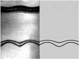
Experimental schlieren images of the evolutions of two successive, quasi-1-D slow/fast interfaces driven by a shock wave are shown in figure 4(a–c) for $L_0=10.0$, 30.0 and 50.0 mm, respectively. Taking the L50-1D case as an example, the wave pattern and interface movement are discussed in detail. After the incident shock wave (IS) impacts the II$_1$, the reflected rarefaction waves (RW$_1$) and the transmitted shock (TS$_1$) are immediately generated, and the shocked upstream interface (SI$_1$) begins to move forwards (116 $\mathrm {\mu }$s). Then the TS$_1$ impacts the II$_2$, and the TS$_2$ is refracted downstream, followed by the shocked downstream interface (SI$_2$) (299 $\mathrm {\mu }$s). Meanwhile, the rarefaction waves (rRW$_2$) are reflected upstream since the II$_2$ is a slow/fast interface relative to the movement of the TS$_1$. After the rRW$_2$ impacts the SI$_1$ (449 $\mathrm {\mu }$s), the transmitted rarefaction waves (tRW$_1$) and reflected rarefaction waves (rRW$_1$) are immediately generated since the SI$_1$ is a fast/slow interface relative to the movement of the rRW$_2$. However, due to the limited strength of the rRW$_1$, the density variation induced by the rRW$_1$ is restricted such that it is challenging to distinguish the rRW$_1$ between the two interfaces. Finally, all waves are refracted away from the two interfaces, and the two interfaces move forward at the same velocity.

Figure 4. Schlieren images of evolutions of two successive, quasi-1-D slow/fast interfaces driven by a shock wave in cases (a) L10-1D, (b) L30-1D and (c) L50-1D, where SI$_1$ (or SI$_2$) denotes the shocked upstream (or downstream) interface, RW$_1$ (or TS$_1$) denotes the reflected rarefaction waves (or transmitted shock) after the IS impacts II$_1$, rRW$_2$ (or TS$_2$) denotes the reflected rarefaction waves (or transmitted shock) after the TS$_1$ impacts II$_2$, and tRW$_1$ denotes the transmitted rarefaction waves after the rRW$_2$ impacts the SI$_1$. Numbers indicate time in $\mathrm {\mu }$s.

The interface displacements ($y_{{SIn}}$) and velocities ($v_{{SIn}}$) of the two interfaces, with $n=1$ for the upstream interface and $n=2$ for the downstream interface, are measured from experiments, as shown in figures 5(a) and 5(b), respectively. Time is scaled as $tv_{{t1}}/L_0$ with $v_{{t1}}$ denoting the velocity of the TS$_1$. Interface displacement is scaled as $(y_{{SIn}}-y_{01})/L_0$, and interface velocity is scaled as $v_{{SIn}}/v_{1}^\alpha$ with $v_{1}^\alpha$ denoting the velocity jump of the upstream interface induced by the IS. The values of $v_{{t1}}$ and $v_{1}^\alpha$ in all cases are calculated according to the 1-D gas dynamics theory (Drake 2018), as listed in table 2. The dimensionless displacements and velocities of the upstream (or downstream) interface converge in all $L_0$ cases, as shown in figure 5(a,b), indicating that the dimensionless movements of the two interfaces are independent of the initial distance between the two interfaces.

Figure 5. The dimensionless (a) displacements and (b) velocities of the upstream interface (solid symbols) and the downstream interface (hollow symbols). Black, yellow and orange solid (or dashed) lines represent the 1-D theory predictions for the upstream (or downstream) interface movements in Stages I, II and III, respectively. The vertical dash–dot lines represent the specific times calculated with (3.1) and (3.9a,b).

Table 2. Physical parameters of the waves and interfaces in the laboratory reference, where $v_{{t1}}$ denotes the velocity of the TS$_1$; $v_{{rRW}_2}$ (or $v_{{rRW_1}}$) denotes the velocity of the rRW$_2$ head (or rRW$_1$ head); $v_{1}^\alpha$ (or $v_{2}^\alpha$) denotes the velocity of the SI$_1$ (or SI$_2$) in Stage I; $v_{1}^\beta$ (or $v_{2}^\beta$) denotes the velocity of the SI$_1$ (or SI$_2$) in Stage II; $v_{fn}$ denotes the asymptotic velocity of the two interfaces; $t_{2}^\alpha$ denotes the specific time when the TS$_1$ impacts the II$_2$; $t_{1}^\beta$ denotes the time when the rRW$_2$ head impacts the SI$_1$ and $t_{2}^\beta$ denotes the time when the rRW$_1$ impacts the SI$_2$; $t_1^\sigma$ (or $t_2^\sigma$) represents the time when the rRW$_2$ (or rRW$_1$) leaves the SI$_1$ (or SI$_2$). The units for velocity and time are m s$^{-1}$ and $\mathrm {\mu }$s, respectively.

3.2. Characteristics of reverberating rarefaction waves

The reverberating rarefaction waves between the two successive slow/fast interfaces are sketched in figure 6. Here, we define the time when the TS$_1$ impacts the II$_2$ as $t_2^\alpha$, the time when the rRW$_2$ impacts the SI$_1$ as $t_1^\beta$, and the time when the rRW$_1$ impacts the SI$_2$ as $t_2^\beta$. Then $t_2^\alpha$, $t_1^\beta$ and $t_2^\beta$ can be derived as

(3.1)\begin{equation} \left. \begin{aligned} t_2^\alpha & =\frac{L_0}{v_{{t1}}},\\ t_1^\beta & =t_2^\alpha+\frac{L_0-t_2^\alpha v_1^\alpha}{v_1^\alpha-v_{{rRW}_2}},\\ t_2^\beta & =t_1^\beta+\frac{L_0-t_2^\alpha v_1^\alpha+(t_1^\beta-t_2^\alpha)(v_2^\alpha-v_1^\alpha)}{v_{{rRW_1}}-v_2^\alpha}, \end{aligned} \right\} \end{equation}

in which $v_2^{\alpha }$ represents the velocity jump of the downstream interface induced by the TS$_1$; $v_{{rRW}_2}$ and $v_{{rRW_1}}$ separately represent the velocity of the rRW$_2$ head and that of the rRW$_1$ head, and they can be stated as

(3.2a,b)\begin{equation} v_{{rRW}_2}=v_1^{\alpha}-c_B^{\alpha},\quad v_{{rRW}_1}=v_2^{\alpha}+c_B^{\beta}, \end{equation}

where $c_B^{\alpha }$ denotes the sound speed of gas B between the TS$_1$ and SI$_1$, and $c_B^{\beta }$ denotes the sound speed of gas B between the rRW$_2$ tail and SI$_2$, as sketched in figure 6(a,b). The values of $v_2^{\alpha }$, $v_{{rRW}_2}$ and $v_{{rRW}_1}$ are calculated according to the 1-D gas dynamics theory (Drake 2018) and (3.2a,b), as listed in table 2. Then $t_2^\alpha$, $t_1^\beta$ and $t_2^\beta$ are calculated based on (3.1), as listed in table 2. As $L_0$ increases, $t_2^\alpha$, $t_1^\beta$ and $t_2^\beta$ increase.

Figure 6. Sketches of (a) the interaction of the TS$_1$ and II$_2$, (b) the interaction of the rRW$_2$ and SI$_1$, (c) the interaction of the rRW$_1$ and SI$_2$, and (d) the movements of the SI$_1$ and SI$_2$ after all waves are refracted away, where $\gamma _A$, $\gamma _B$ and $\gamma _C$ denote the specific heat ratios of gas A, gas B and gas C, respectively; $c_A$ denotes the sound speed of gas A after the IS impacts the II$_1$, $c_B^\alpha$ denotes the sound speed of gas B between the TS$_1$ with the II$_2$, $c_B^\beta$ denotes the sound speed of gas B between the rRW$_2$ tail and the SI$_2$, $c_B^\sigma$ denotes the sound speed of gas B between the rRW$_1$ tail and the SI$_1$, $c_C$ denotes the sound speed of gas C behind TS$_2$; $p_1$ denotes the pressure of gas B behind the TS$_1$, $p_2$ denotes the pressure of gas B behind the rRW$_2$ tail, $p_3$ denotes the pressure of gas B behind the rRW$_1$ tail, and $p_4$ denotes the pressure of gas B after the interaction of the rRW$_1$ and SI$_2$. (a) $t=t_2^\alpha$, (b) $t=t_1^\beta$, (c) $t=t_2^\beta$, (d) $t>t_2^\beta$.

After the rRW$_2$ impacts the SI$_1$, the velocity of the SI$_1$ increases from $v_1^\alpha$ to $v_1^\beta$ since the pressure behind the rRW$_2$ tail ($p_2$) is lower than the pressure in front of the rRW$_2$ head ($p_1$), as sketched in figure 6(a,b). Differently, after the rRW$_1$ impacts the SI$_2$, the velocity of the SI$_2$ reduces from $v_2^\alpha$ to $v_2^\beta$ since the pressure behind the rRW$_1$ tail ($p_3$) is lower than $p_2$, as sketched in figure 6(b,c). The solutions of $v_1^\beta$ and $v_2^\beta$ are discussed in detail.

First, based on the 1-D gas dynamics theory for the interaction of rarefaction waves and a fast/slow interface (Drake 2018; Liang & Luo 2022a), $v_1^{\beta }$ can be solved as

(3.3)\begin{equation} v_1^{\beta}=v_1^{\alpha}-\frac{2c_A}{\gamma_A-1}\left[\,p_{31}^{(\gamma_A-1)/2\gamma_A}-1\right], \end{equation}

where $\gamma _A$ is the specific heat ratio of gas A, and $c_A$ is the sound speed of gas A after the IS impacts the II$_1$, as sketched in figure 6(a). The only unknown parameter $\,p_{31}$, i.e. the ratio of the $p_3$ to $p_1$, satisfies

(3.4)\begin{equation} \frac{c_A}{c_B^{\alpha}}=\frac{(\gamma_A-1)\left[\,p_{31}^{(\gamma_B-1)/2\gamma_B}-2\,p_{21}^{(\gamma_B-1)/2\gamma_B}+1\right]}{(\gamma_B-1)\left[1-\,p_{31}^{(\gamma_A-1)/2\gamma_A}\right]}, \end{equation}

where $\gamma _B$ is the specific heat ratio of gas B, $c_B^\alpha$ is the sound speed of gas B between the TS$_1$ with the II$_2$, and $\,p_{21}$ is the ratio of $p_2$ to $p_1$. Then $v_1^\beta$ in all cases can be calculated by solving (3.3)–(3.4), as listed in table 2.

Second, based on the 1-D gas dynamics theory for the interaction of rarefaction waves and a slow/fast interface (Drake 2018; Liang & Luo 2021a), $v_2^{\beta }$ can be calculated as

(3.5)\begin{equation} v_{2}^\beta=v_{2}^\alpha+\frac{2c_B^\beta}{\gamma_B-1}\left[(\,p_{32})^{(\gamma_B-1)/2\gamma_B}-1\right]-\frac{\sqrt{2}c_B^\beta(\,p_{42}/p_{32}-1)}{\sqrt{\gamma_B(\gamma_B+1)\,p_{42}/p_{32}}}, \end{equation}

where $c_B^\beta$ is the sound speed of gas B between the rRW$_2$ tail and the SI$_2$, and $\,p_{32}$ is the ratio of $p_3$ to $p_2$. The only unknown parameter $\,p_{42}$, i.e. the ratio of the pressure of the flow after the rRW$_1$ leaves the SI$_2$ ($p_4$) to $p_2$, satisfies

(3.6)\begin{equation} \frac{c_C}{c_B^\beta}=\frac{\gamma_C-1}{\,p_{42}^{(\gamma_C-1)/2\gamma_C}-1} \left\{\frac{2}{\gamma_B-1}\left[\,p_{32}^{(\gamma_B-1)/2\gamma_B}-1\right] -\frac{\sqrt{2}(\,p_{42}/p_{32}-1)\,p_{32}^{(\gamma_B-1)/2\gamma_B}} {\sqrt{(\gamma_B+1)\gamma_B\,p_{42}/p_{32}+(\gamma_B-1)\gamma_B}}\right\}, \end{equation}

where $c_C$ is the sound speed of gas C after the TS$_1$ impacts the II$_2$, and $\gamma _C$ is the specific heat ratio of gas C. Then $v_{2}^\beta$ in all cases can be calculated by solving (3.5)–(3.6), as listed in table 2.

We note that the number of reverberating waves between the two interfaces should be infinite. However, the consecutive pressure and velocity changes imparted by these reverberations decrease, eventually converging to a well-defined asymptotic 1-D post-shock state. The influences of the reverberating waves on the 1-D and 2-D dynamics of the two interfaces should be considered until the two interfaces enter the asymptotic post-shock state (Aglitskiy et al. 2006; Liang & Luo 2022a). A simple and advantageous method is adopted to judge whether the higher-order reverberations should be accounted for or not. The interaction of an incident shock wave with a semi-infinite interface separating two fluids with $\rho _A$ and $\rho _C$ is considered, ignoring the intermediate layer of gas B. The post-shock final velocity, $v_{{fn}}$, is calculated according to the 1-D gas dynamics theory (Drake 2018), as listed in table 2. The differences among the $v_1^\beta$, $v_2^\beta$ and $v_{{fn}}$ are limited: $v_{{fn}}$ is only 0.2 % smaller than $v_1^\beta$ and 0.1 % larger than $v_2^\beta$. Therefore, it is reasonable to regard that after the rRW$_1$ impacts the SI$_2$, the movements of the two interfaces enter the asymptotic state.

The interaction between rarefaction waves and an interface is a continuous process (Li & Book 1991; Li, Kailasanath & Book 1991; Morgan, Likhachev & Jacobs 2016; Morgan et al. 2018; Liang et al. 2020b; Wang et al. 2022). The length of the rRW$_2$ at $t_1^\beta$ ($L_{rRW_2}$), the interaction time of the rRW$_2$ with the SI$_1$ ($T_{{rRW_2}}$), and the average acceleration imposed on the SI$_1$ by the rRW$_2$ ($\bar {g}_{{rRW_2}}$) are respectively deduced as

(3.7)\begin{equation} \left. \begin{aligned} L_{rRW_2} & =(c_B^\alpha+v_2^\alpha-c_B^\beta-v_1^\alpha)(t_1^\beta-t_2^\alpha),\\ T_{{rRW_2}} & =\frac{2L_{rRW_2}}{2(c_B^\beta-v_2^\alpha)+v_1^\alpha+v_1^\beta},\\ \bar{g}_{{rRW_2}} & =\frac{v_1^\beta-v_1^\alpha}{T_{{rRW_2}}}. \end{aligned} \right\} \end{equation}

Similarly, the length of the rRW$_1$ at $t_2^\beta$ ($L_{rRW_1}$), the interaction time of the rRW$_1$ with the SI$_2$ ($T_{{rRW_1}}$), and the average deceleration imposed on the SI$_2$ by the rRW$_1$ ($\bar {g}_{{rRW_1}}$) are respectively derived as

(3.8)\begin{equation} \left. \begin{aligned} L_{rRW_1} & =(c_B^\beta+v_2^\alpha-c_B^\sigma-v_1^\beta)(t_2^\beta-t_1^\beta),\\ T_{{rRW_1}} & =\frac{2L_{rRW_1}}{2(c_B^\sigma+v_1^\beta)-v_2^\alpha-v_2^\beta},\\ \bar{g}_{{rRW_1}} & =\frac{v_2^\beta-v_2^\alpha}{T_{{rRW_1}}}, \end{aligned} \right\} \end{equation}

in which $c_B^\sigma$ ($=c_B^\beta -(\gamma _B-1)(u_2^\alpha -u_1^\beta )/2$) is the sound speed of gas B behind the rRW$_1$, as sketched in figure 6(c). The values of $L_{rRW_2}$, $T_{{rRW_2}}$ and $\bar {g}_{{rRW_2}}$ in all cases are calculated based on (3.7), and the values of $L_{rRW_1}$, $T_{{rRW_1}}$ and $\bar {g}_{{rRW_1}}$ in all cases are calculated according to (3.8), as listed in table 3. As $L_0$ increases, $L_{rRW_2}$, $L_{rRW_1}$, $T_{{rRW_2}}$ and $T_{{rRW_1}}$ increase, whereas both $\bar {g}_{{rRW_2}}$ and $|\bar {g}_{{rRW_1}}|$ decrease.

Table 3. Physical parameters of the reverberating rarefaction waves, where $L_{rRW_2}$ denotes the length of the rRW$_2$ at $t_1^\beta$, $T_{{rRW_2}}$ denotes the interaction time of the rRW$_2$ and the SI$_1$, $\bar {g}_{{rRW_2}}$ denotes the average acceleration imposed on the SI$_1$ by the rRW$_2$, $L_{rRW_1}$ denotes the length of the rRW$_1$ at $t_2^\beta$, $T_{{rRW_1}}$ denotes the interaction time of the rRW$_1$ and the SI$_2$, and $\bar {g}_{{rRW_1}}$ denotes the average deceleration imposed on the SI$_2$ by the rRW$_1$. The units for length, time and acceleration are mm, $\mathrm {\mu }$s and $10^6\ \textrm {m}\ \textrm {s}^{-2}$, respectively.

In summary, the shocked two successive slow/fast interfaces’ movements can be separated into Stages I, II and III, as listed in table 4, where $t_1^\sigma$ (or $t_2^\sigma$) represents the time when the rRW$_2$ (or rRW$_1$) leaves the SI$_1$ (or SI$_2$),

(3.9a,b)\begin{equation} t_1^\sigma=t_1^\beta+T_{{rRW_2}},\quad t_2^\sigma=t_2^\beta+T_{{rRW_1}}. \end{equation}

As a result, a general 1-D theory is established to describe the movements of the two interfaces based on the derived specific times ((3.1) and (3.9a,b)) and interface velocities ((3.2a,b)–(3.8)). The predictions of the 1-D theory for the interface movements in Stages I, II and III are marked with black, yellow and orange lines, respectively, as shown with solid lines for the upstream interface and dashed lines for the downstream interface in figure 5(a,b), and they agree well with the experimental results. Significantly, the specific times when the reverberating waves impact the two interfaces (e.g. $t_1^\beta$, $t_1^\sigma$, $t_2^\beta$, and $t_2^\sigma$) and the velocity jumps at these moments predicted by the 1-D gas dynamic theory agree well with the experiments.

Table 4. The movements of the shocked two successive slow/fast interfaces in different stages, where ‘Uni.’ is short for ‘Uniform movement’, ‘Acc.’ is short for ‘Acceleration movement’ and ‘Dec.’ is short for ‘Deceleration movement’.

4. Quasi-2-D hydrodynamic instabilities

We shall first examine the deformations of the two interfaces observed from experimental and numerical schlieren images. The amplitude growth rates are then acquired from the experiments and simulations. Next, an analytical, linear model is further extended by considering the arbitrary wavenumber and phase combinations and compressibility, which successfully describes the RMI of the two successive slow/fast interfaces. Later, the influences of the reverberating rarefaction waves on the hydrodynamic instabilities of the two interfaces are quantified. Last, the conditions and outcomes of the freeze-out and abnormal RMI are summarised.

4.1. Experimental and numerical results

Schlieren images of the shock-induced two successive slow/fast interface evolutions acquired from experiments and simulations are shown in figure 7(a–f). The magnitude of the density gradient ($\boldsymbol {\nabla }\rho$) field in the simulations is calculated as (Quirk & Karni 1996; Sembian, Liverts & Apazidis 2018)

(4.1)\begin{equation} |\boldsymbol{\nabla}\rho|=\left[\left(\frac{\partial\rho}{\partial x}\right)^2+\left(\frac{\partial\rho}{\partial y}\right)^2\right]^{{1}/{2}}. \end{equation}

Taking the L50-IP case as an example, the deformations of the two interfaces are discussed in detail. After the IS impacts the perturbed II$_1$, the rippled RW$_1$ is reflected upstream, and the rippled TS$_1$ moves towards the II$_2$ (121 $\mathrm {\mu }$s). Meanwhile, the perturbation on the SI$_1$ decreases due to phase reversal (Brouillette 2002). After the TS$_1$ impacts the perturbed II$_2$, the rippled TS$_2$ is refracted downstream, and the rippled rRW$_2$ is reflected towards the SI$_1$ (304 $\mathrm {\mu }$s). Meanwhile, the perturbation on the SI$_2$ decreases due to phase reversal (Brouillette 2002). After the rRW$_2$ impacts the SI$_1$, the tRW$_1$ is refracted upstream (454 $\mathrm {\mu }$s) and, theoretically, the rRW$_1$ is reflected towards the SI$_2$. Finally, the perturbations on the two interfaces increase gradually with phases opposite to their initial perturbations.

Figure 7. Schlieren images of evolutions of quasi-2-D two successive slow/fast interfaces driven by a shock wave acquired from experiments (upper) and simulations (below) in cases (a) L10-IP, (b) L10-AP, (c) L30-IP, (d) L30-AP, (e) L50-IP and (f) L50-AP. The upstream interface in panel (b) is highlighted with a white dashed line. Although the upstream interface in panel (b) is a slow/fast one, it does not experience phase reversal. Numbers denote time in $\mathrm {\mu }$s.

In addition, we observe that the SI$_1$ in the L10-AP case does not experience phase reversal (see the white dashed lines in figure 7b), which is different from the other cases and the RMI of a semi-infinite slow/fast interface reported before (Jourdan & Houas 2005; Mariani et al. 2008). The phenomena, including the perturbation of a shocked slow/fast interface growing with the same phase as its initial state and the perturbation of a shocked fast/slow interface growing with the opposite phase as its initial state, are called ‘abnormal RMI’. This study is the first to provide observational evidence of the abnormal RMI.

The amplitude growth rate of the upstream interface obtained from experiments ($\dot {a}_1^{{exp}}$) and simulations ($\dot {a}_1^{{num}}$), and that of the downstream interface obtained from experiments ($\dot {a}_2^{{exp}}$) and simulations ($\dot {a}_2^{{num}}$) in Stage I are acquired by linearly fitting the quantitative data, as listed in table 5. First, it is found that $\dot {a}_1^{{num}}$ and $\dot {a}_2^{{num}}$ separately agree well with $\dot {a}_1^{{exp}}$ and $\dot {a}_2^{{exp}}$ within the experimental measurement errors, further validating the code adopted in this study. Second, in the three in-phase cases, as $L_0$ increases, both $|\dot {a}_1^{{exp}}|$ and $|\dot {a}_2^{{exp}}|$ decrease. However, in the three anti-phase cases, as $L_0$ increases, both $|\dot {a}_1^{{exp}}|$ and $|\dot {a}_2^{{exp}}|$ increase. The results indicate that the RMI of two successive interfaces is influenced by the initial distance and perturbations of the two interfaces, i.e. the feedthrough between the two interfaces. Third, due to the feedthrough effect, the sign of $\dot {a}_1^{{exp}}$ is the same as the sign of $a_1(0)$ in the L10-AP case, which goes against the classical RMI where the sign of the amplitude growth rate of a semi-infinite slow/fast interface is opposite to the sign of its initial perturbation (Jourdan & Houas 2005; Mariani et al. 2008). As we mentioned above, this is called abnormal RMI. Unlike the present results, an opposite amplitude growth rate to the initial perturbation amplitude of a fast/slow interface was found by Liang & Luo (2022a). Therefore, the outcomes of the abnormal RMI are dependent on the fluid distribution.

Table 5. The linear amplitude growth rates of the two interfaces, where $\dot {a}_1^{{exp}}$, $\dot {a}_1^{{num}}$ and $\dot {a}_1^{{lin}}$ denote the experimental, numerical and theoretical results of the upstream interface, respectively; $\dot {a}_2^{{exp}}$, $\dot {a}_2^{{num}}$ and $\dot {a}_2^{{lin}}$ denote the experimental, numerical and theoretical results of the downstream interface, respectively; and $\psi _1$ and $\psi _2$ denote the feedthrough effect on the RMI of the upstream and downstream interfaces, respectively.

4.2. The feedthrough effect on the RMI

Because the influences of the feedthrough and reverberating rarefaction waves on the hydrodynamic instabilities of the two interfaces are coupled, it is essential to quantify the two effects separately and analytically. Based on the linear stability analysis, Liang & Luo (2022a) deduced a linear model for evaluating the amplitude growth rates of the upstream interface ($\dot {a}_1^{{lin}}$) and downstream interface ($\dot {a}_2^{{lin}}$) owning the same wavenumber ($k$) as

(4.2)\begin{equation} \left. \begin{aligned} & \dot{a}_1^{{lin}}=\frac{kv_1^{\alpha} \left[Z_1a_1(0)(1-R_1)(2R_3\xi+\xi^2+1)+Z_2a_2(0)(R_3-1)(1-\xi^2)\right]}{2\xi(R_1R_3+1)+(R_1+R_3)(\xi^2+1)},\\ & \dot{a}_2^{{lin}}=\frac{kv_2^{\alpha} \left[Z_1a_1(0)(R_1-1)(\xi^2-1)+Z_2a_2(0)(R_3-1)(2R_1\xi+\xi^2+1)\right]}{2\xi(R_1R_3+1)+(R_1+R_3)(\xi^2+1)}, \end{aligned} \right\} \end{equation}

in which three compression factors $Z_1$ ($=1-v_1^\alpha /v_{s}$), $Z_2$ ($=1-v_2^\alpha /v_{{t1}}$) and $Z_L$ ($=1-v_1^\alpha /v_{{t1}}$) are introduced; $\xi =\tanh (kh_0)$ and $h_0=Z_LL_0/2$ are included. However, this model can only quantify the RMI of two successive fast/slow interfaces with the same wavenumber and initially in-phase or anti-phase perturbations. In this work, we extend the linear model by considering the arbitrary wavenumber and phase combinations and compressibility.

We set the single-mode perturbation on the initial upstream interface as $\eta _1(0)=a_1(0)\cos (k_1x)$ and the single-mode perturbation on the initial downstream interface as $\eta _2(0)=a_2(0)\cos (k_2x+\theta )$, where $\theta$ represents the phase difference between the two interfaces’ perturbations. If there is no perturbation on the downstream interface, then the amplitude growth rates of the two interfaces at $x=0$ are

(4.3)\begin{equation} \left. \begin{aligned} & \dot{a}_1^{{lin}}(a_1(0),0)=\frac{k_1v_1^{\alpha}Z_1a_1(0)(1-R_1)(2R_3\xi+\xi^2+1)}{2\xi(R_1R_3+1)+(R_1+R_3)(\xi^2+1)},\\ & \dot{a}_2^{{lin}}(a_1(0),0)=\frac{k_1v_2^{\alpha}Z_1a_1(0)(R_1-1)(\xi^2-1)\cos(\theta)}{2\xi(R_1R_3+1)+(R_1+R_3)(\xi^2+1)}. \end{aligned} \right\} \end{equation}

If there is no perturbation on the upstream interface, then the amplitude growth rates of the two interfaces at $x=-\theta /k_2$ are

(4.4)\begin{equation} \left. \begin{aligned} & \dot{a}_1^{{lin}}(0,a_2(0))=\frac{k_2v_1^{\alpha}Z_2a_2(0)(R_3-1)(1-\xi^2)\cos(\theta)}{2\xi(R_1R_3+1)+(R_1+R_3)(\xi^2+1)},\\ & \dot{a}_2^{{lin}}(0,a_2(0))=\frac{k_2v_2^{\alpha}Z_2a_2(0)(R_3-1)(2R_1\xi+\xi^2+1)}{2\xi(R_1R_3+1)+(R_1+R_3)(\xi^2+1)}. \end{aligned} \right\} \end{equation}

Based on the linear superposition principle, if there are perturbations imposed on the two initial interfaces simultaneously, then the amplitude growth rates of the two interfaces can be derived by superposing (4.3) and (4.4) as

(4.5)\begin{equation} \dot{a}_1^{{lin}}=\psi_1\dot{a}_1^{SI},~\dot{a}_2^{{lin}}=\psi_2\dot{a}_2^{SI}, \end{equation}

in which $\dot {a}_1^{SI}$ and $\dot {a}_2^{SI}$ denote the linear amplitude growth rates of the upstream interface and downstream interface when they are semi-infinite, respectively; and $\psi _1$ and $\psi _2$ quantify the feedthrough effect on the RMI of the upstream and downstream interfaces, respectively,

(4.6)\begin{equation} \left. \begin{aligned} & \psi_1 = \frac{(R_1 + 1)(2R_3\xi + \xi^2 + 1) - (R_1 + 1)(R_3 - 1)(1 - \xi^2)\cos(\theta)/[\kappa(R_1 - 1)]}{2\xi(R_1R_3 + 1) + (R_1 + R_3)(\xi^2 + 1)},\\ & \psi_2 = \frac{\kappa(R_1 - 1)(R_3 + 1)(\xi^2 - 1)\cos(\theta)/(R_3 - 1) + (R_3 + 1)(2R_1\xi + \xi^2 + 1)}{2\xi(R_1R_3 + 1) + (R_1 + R_3)(\xi^2 + 1)}, \end{aligned} \right\} \end{equation}

with $\kappa =k_1Z_1a_1(0)/k_2Z_2a_2(0)$.

Liang & Luo (2022a) adopted the original prescription introduced by Richtmyer (1960) to evaluate $\dot {a}_1^{SI}$ and $\dot {a}_2^{SI}$ considering the shock-reflected case in incompressible flow,

(4.7a,b)\begin{equation} \dot{a}_1^{SI}=k_1Z_1a_1(0)v_1^{\alpha}A_1,\quad \dot{a}_2^{SI}=k_2Z_2a_2(0)v_2^{\alpha}A_2. \end{equation}

Therefore, the original linear model only applies to two successive fast/slow interfaces in the weak-shock limit. In this work, we extend the linear model considering the compressibility by using the linearised compressible solution for a shocked slow/fast interface introduced by Wouchuk & Nishihara (1996, 1997). Then, the expressions of $\dot {a}_1^{SI}$ and $\dot {a}_2^{SI}$ can be written as

(4.8)\begin{equation} \left. \begin{aligned} & \dot{a}_1^{SI}=k_1a_1(0)v_1^{\alpha}\frac{v_{{IS}}-v_{{t1}} -R_1(1-v_{{ps}})(v_{{IS}}+c_A-v_1^{\alpha}) }{(R_1+1)v_{{IS}}},\\ & \dot{a}_2^{SI}=k_2a_2(0)v_2^{\alpha}\frac{v_{{t1}}-v_{{t2}} -R_3(1-v_1^{\alpha})(v_{{t1}}+c_B^{\beta}-v_2^{\alpha}) }{(R_3+1)v_{{t1}}}, \end{aligned} \right\} \end{equation}

in which $v_{{t2}}$ denotes the velocity of the TS$_2$. Equation (4.8) not only quantifies the baroclinic contribution to the vorticity but also considers the tangential velocity perturbations along the contact surface separately generated by the corrugated transmitted shock and the corrugated rarefaction waves.

Moreover, Liang & Luo (2022a) concluded that the feedthrough effect on RMI is partially related to the amplitude ratio of the two interfaces, which is not rigorous. From (4.6), it is noted that the feedthrough $\psi$ is not only related to the density ratios $R_1$ and $R_3$, the dimensionless distance $\xi$ and the phase difference $\theta$, but is also related to the ratio of the products of the wavenumber and amplitude of the two interfaces $\kappa$.

The values of $\dot {a}_1^{{lin}}$ and $\dot {a}_2^{{lin}}$ are calculated with the extended linear model (i.e. (4.5)–(4.8)) and listed in table 5. It can be seen that they agree well with all experimental and numerical results. Notably, the extended linear model successfully predicts the abnormal RMI of the upstream interface in the L10-AP case. Therefore, the extended linear model is proved to be applicable for describing the RMI of two successive slow/fast interfaces with various initial conditions.

The values of $\psi _1$ and $\psi _2$ in all experimental cases are listed in table 5. In the L10-AP case, $\psi _1<0$ indicates the abnormal RMI of the upstream interface caused by the feedthrough. Moreover, it is found that $|\psi _1|>1$ and $|\psi _2|>1$ in the three in-phase cases and $|\psi _1|<1$ and $|\psi _2|<1$ in the three anti-phase cases, indicating that the feedthrough leads to the two in-phase slow/fast interfaces being more unstable and the two anti-phase slow/fast interfaces being more stable in the six experimental cases. However, this conclusion is not rigorously applied to all possibilities. Some exceptions are found under specific initial conditions. The values of $\psi$ versus $kh_0$ under different $\kappa$ conditions when the two interfaces are initially in-phase and anti-phase are calculated based on (4.6), as shown in figures 8(a) and 8(b), respectively. It is found that when $kh_0>2$, the feedthrough has negligible influence on the RMI of the two interfaces.

Figure 8. The values of $\psi$ versus $kh_0$ under different $\kappa$ conditions when (a) $\theta =0$ and (b) $\theta ={\rm \pi}$. Hollow circles represent the instability freeze-out of the upstream or downstream interface.

In figure 8(a), we plot $\psi _1$ and $\psi _2$ as functions of $kh_0$ for the case $\kappa$ varying from 0.1 to 10.0, $R_1=1.5$, $R_3=0.5$ and $\theta =0$. It is found that when $kh_0<2$, except for the $\kappa =0.1$ case, $\psi _1>1$ and $\psi _2>1$, indicating that the feedthrough results in the two interfaces being more unstable. However, when $\kappa$ and $kh_0$ are limited (e.g. $\kappa =0.1$ and $kh_0<1$), $\psi _1>1$ and $1>\psi _2>0$, demonstrating that the feedthrough leads to the upstream interface being more unstable and the downstream interface being more stable. Therefore, the two successive interfaces with initially in-phase perturbations are generally destabilised by the feedthrough, but the downstream interface might be stabilised if $\kappa$ is limited.

In figure 8(b), we plot $\psi _1$ and $\psi _2$ as functions of $kh_0$ for the case $\kappa$ varying from 0.1 to 10.0, $R_1=1.5$, $R_3=0.5$ and $\theta ={\rm \pi}$. First, $\psi _1=0$ or/and $\psi _2=0$ under specific $kh_0$ conditions demonstrate that the feedthrough might cause the RMI of the upstream interface or/and the downstream interface to be frozen. Notably, the freeze-out RMI concerned in this study is caused by the feedthrough between the two interfaces, not the compressibility as discussed by previous studies (Fraley 1986; Mikaelian 1993, 1994; Wouchuk & Nishihara 1997, 2004; Wouchuk & Sano 2015). Moreover, $\psi _1<0$ or $\psi _2<0$ demonstrates that the abnormal RMI of the upstream interface or downstream interface occurs. Although the two slow/fast interfaces are initially anti-phase, $|\psi _1|>1$ under the small $\kappa$ condition (e.g. $\kappa =0.1$ and 0.5) indicates the RMI of the upstream interface is promoted, and $|\psi _2|>1$ under the large $\kappa$ condition (e.g. $\kappa =10.0$) indicates the RMI of the downstream interface is promoted.

Overall, the feedthrough generally leads to the two in-phase slow/fast interfaces being more unstable and the two anti-phase slow/fast interfaces being more stable, but there are exceptions under specific conditions: first, the downstream one of the two initially in-phase interfaces might be stabilised if $\kappa$ is limited; second, the upstream one of the two initially anti-phase interfaces might be destabilised if $\kappa$ is limited; third, the downstream one of the two initially anti-phase interfaces might be destabilised if $\kappa$ is large. It is evident that the freeze-out and abnormal RMI complicate the analysis of the hydrodynamic instabilities of the two interfaces and will be discussed in detail later.

4.3. The reverberating rarefaction waves effect

The time-varying amplitudes of the upstream interface and downstream interface are scaled to eliminate the feedthrough effect and highlight the reverberating rarefaction waves effect, as shown in figures 9(a) and 9(b), respectively. For the upstream interface, time is scaled as $\tau _1=|k_1\dot {a}_1^{{lin}}t|$ and amplitude is scaled as $\eta _1=|k_1a_1|$. For the downstream interface, time is scaled as $\tau _2=|k_2\dot {a}_2^{{lin}}(t-t_2^\alpha )|$ and amplitude is scaled as $\eta _2=|k_2a_2|$. Except for $\eta _1$ in the L10-AP case, both $\eta _1$ and $\eta _2$ decrease to zero at first due to phase reversal (Brouillette 2002) and then increase. The rarefaction waves have short-time influences on the hydrodynamic instabilities due to the short duration times of the interaction of the rarefaction waves and the two interfaces in this study (see $T_{{rRW}_2}$ and $T_{{rRW}_1}$ in table 3). However, it is found that the perturbation of the upstream interface in the L10-AP case is suddenly stretched by the rRW$_2$, as seen in the inset of figure 9(a). The rarefaction waves influence the hydrodynamic instabilities of the two interfaces in two ways: on the one hand, the rarefaction waves stretch the two interfaces in the streamwise direction during the interaction; on the other hand, the rarefaction waves impose the short-time RTI or RTS on the two interfaces since the interaction of the rarefaction waves and an interface is not instantaneous but a process (Li & Book 1991; Li et al. 1991; Morgan et al. 2016, 2018; Liang et al. 2020b; Wang et al. 2022).

Figure 9. The time-varying dimensionless amplitudes of the (a) upstream interface and (b) downstream interface obtained from experiments.

To simplify the analysis, the interaction of 1-D rarefaction waves and 2-D interfaces are considered. For the upstream interface, since the rRW$_2$ accelerates the spike then the bubble of the upstream interface, the rRW$_2$ stretches the perturbation of the upstream interface during the interaction. The amplitude of the upstream interface when the rRW$_2$ head impacts the upstream interface is $a_1^\beta$ ($=Z_1a_1(0)+\dot {a}_1^{{lin}}t_1^\beta$), the relative velocity difference between the upstream interface and the rRW$_2$ is $c_B^\alpha$, and the upstream interface velocity increment induced by the rRW$_2$ is ($v_1^\beta -v_1^\alpha$). Therefore, the time-varying stretching effect of rRW$_2$ on the upstream interface amplitude ($a_{{rRW_2}}$) is

(4.9)\begin{equation} a_{{rRW_2}}=\frac{(v_1^\beta-v_1^\alpha)(t-t_1^\beta+a_1^\beta/c_B^\alpha)}{2}, \end{equation}

with $(t_1^\beta +a_1^\beta /c_B^\alpha )>t>(t_1^\beta -a_1^\beta /c_B^\alpha )$.

For the downstream interface, since the rRW$_1$ decelerates the bubble tip then the spike tip of the downstream interface, the rRW$_1$ also stretches the perturbation of the downstream interface during the interaction. The amplitude of the downstream interface when the rRW$_1$ head impacts the downstream interface is $a_2^\beta$ ($=Z_2a_2(0)+\dot {a}_2^{{lin}}(t_2^\beta -t_2^\alpha )$), the relative velocity difference between the downstream interface and the rRW$_1$ is $c_B^\beta$, and the downstream interface velocity decrement induced by the rRW$_1$ is ($v_2^\alpha -v_2^\beta$). Therefore, the time-varying stretching effect of rRW$_1$ on the downstream interface amplitude ($a_{{rRW_1}}$) is

(4.10)\begin{equation} a_{{rRW_1}}=\frac{(v_2^\alpha-v_1^\beta)(t-t_2^\beta+a_2^\beta/c_B^\beta)}{2}, \end{equation}

with $(t_2^\beta +a_2^\beta /c_B^\beta )>t>(t_2^\beta -a_2^\beta /c_B^\beta )$.

Except for the freeze-out and abnormal RMI cases, the two slow/fast interfaces generally experience phase reversal, resulting in the difficulty of modelling the additional instabilities imposed by the rarefaction waves on the two interfaces. Since the post-shock amplitude of the upstream (or downstream) interface is $Z_1a_1(0)$ (or $Z_2a_2(0)$) and the perturbation amplitude of the upstream (or downstream) interface decreases at a linear rate ${\dot {a}}_1^{{lin}}$ (or ${\dot {a}}_2^{{lin}}$), the time when the perturbation of the upstream (or downstream) interface decreases to zero, i.e. the end time of the phase reversal of the upstream (or downstream) interface $t_1^{{pr}}$ (or $t_2^{{pr}}$), can be evaluated as

(4.11a,b)\begin{equation} t_1^{{pr}}=|Z_1a_1(0)/\dot{a}_1^{{lin}}|,\quad t_2^{{pr}}=t_2^\alpha+|Z_2a_2(0)/\dot{a}_2^{{lin}}|. \end{equation}

The values of $t_1^{{pr}}$ and $t_2^{{pr}}$ in all cases are listed in table 6. On comparing $t_1^{{pr}}$ with $t_1^{\beta }$ in table 2, it is found $t_1^{{pr}}>t_1^{\beta }$ in all cases except for the case L10-AP, indicating that the rRW$_2$ impacts the upstream interface before the end of the upstream interface's phase reversal. Because of the baroclinic vorticity created by the misalignment of the density gradient ($\boldsymbol {\nabla }\rho$) and the pressure gradient ($\boldsymbol {\nabla } p$), the rRW$_2$ continuously deposits the vorticity with the same direction as the vorticity deposited by the IS on the upstream interface, as sketched in figure 10(a). Therefore, the rRW$_2$ imposes the short-time RTI on the upstream interface, resulting in the upstream interface being more unstable. Due to the abnormal RMI in the L10-AP case, the vorticity deposited on the upstream interface by the IS is opposite to that in other cases, as sketched in figure 10(b). As a result, the rRW$_2$ imposes the short-time RTS on the upstream interface in the L10-AP case, leading to the upstream interface being more stable.

Table 6. The end times of the upstream (or downstream) interface's phase reversal $t_1^{{pr}}$ (or $t_2^{{pr}}$) calculated with (4.11a,b). The unit of time is $\mathrm {\mu }$s.

Figure 10. Sketches of (a) the interaction of the rRW$_2$ and SI$_1$ in all cases (except for the L10-AP case), (b) the interaction of the rRW$_2$ and SI$_1$ in the L10-AP case, (c) the interaction of the rRW$_1$ and SI$_2$ under $L_0=10.0$ and 30.0 mm conditions, and (d) the interaction of the rRW$_1$ and SI$_2$ under $L_0=50.0$ mm conditions. The blue (or orange) arcs with an arrow in panels (a,b) illustrate the vorticity deposited by the IS (or rRW$_2$) on the upstream interface. The blue (or orange) arcs with an arrow in panels (c,d) represent the vorticity deposited by the TS$_1$ (or rRW$_1$) on the downstream interface. The purple (or green) arrows represent the pressure (or density) gradient $\boldsymbol {\nabla } p$ (or $\boldsymbol {\nabla }\rho$).

Similarly, by comparing $t_2^{{pr}}$ with $t_2^{\beta }$ in table 2, it is found that $t_2^{{pr}}>t_2^{\beta }$ under $L_0=10.0$ and 30.0 mm conditions and $t_2^{{pr}}< t_2^{\beta }$ under $L_0=50.0$ mm conditions. In other words, the rRW$_1$ impacts the downstream interface before the end of the downstream interface's phase reversal under $L_0=10.0$ and 30.0 mm conditions, depositing the vorticity in the opposite direction to the vorticity deposited by the TS$_1$ on the upstream interface, as sketched in figure 10(c). In contrast, the rRW$_1$ impacts the downstream interface after the downstream interface's phase reversal under $L_0=50.0$ mm conditions, depositing the vorticity with the same direction as the vorticity deposited by the TS$_1$ on the downstream interface, as sketched in figure 10(d). As a result, the rRW$_1$ imposes the short-time RTS on the downstream interface, resulting in the downstream interface being more stable under $L_0=10.0$ and 30.0 mm conditions. In contrast, the rRW$_1$ imposes the short-time RTI on the downstream interface, leading to the upstream interface being more unstable under $L_0=50.0$ mm conditions.

Here, we modify the nonlinear model proposed by Zhang & Guo (2016), considering the universal curves of all spikes and bubbles at any density ratio, to quantify the short-time RTI or RTS imposed by the rRW$_2$ on the upstream interface and that imposed by the rRW$_1$ on the downstream interface. The expressions of the modified nonlinear model for the bubble/spike amplitude growth rate of the upstream interface ($\dot {a}_{1b/1s}$) and the downstream interface ($\dot {a}_{2b/2s}$) in Stage II are

(4.12)\begin{equation} \ddot{a}_{ns/nb}=({-}1)^i\alpha_{ns/nb}k_n\left[(\dot{a}_{ns/nb})^{2}-(\dot{a}_{ns/nb}^{qs})^2\right]. \end{equation}

For the upstream interface, $i=0$ when $t_1^{{pr}}>t_1^{\beta }$ or $\psi _1<0$, and $i=1$ when $t_1^{{pr}}< t_1^{\beta }$; for the downstream interface, $i=0$ when $t_2^{{pr}}< t_2^{\beta }$ or $\psi _2<0$, and $i=1$ when $t_2^{{pr}}>t_2^{\beta }$;

(4.13)\begin{equation} \dot{a}_{ns/nb}^{qs}=\sqrt{\frac{|A_n\bar{g}_{{rRW_{(3-n)}}}|}{3k_n}\frac{8}{(1\pm A_n)(3\pm A_n)}\frac{\left[3\pm A_n+\sqrt{2(1\pm A_n)}\right]^{2}}{\left[4(3\pm A_n)+\sqrt{2(1\pm A_n)}(9\pm A_n)\right]}}, \end{equation}

and

(4.14)\begin{equation} \alpha_{ns/nb}=\frac{3}{4}\frac{(1\pm A_n)(3\pm A_n)}{\left[3\pm A_n+\sqrt{2(1\pm A_n)}\right]}\frac{\left[4(3\pm A_n)+\sqrt{2(1\pm A_n)}(9\pm A_n)\right]}{\left[\sqrt{3\pm A_n}+2\sqrt{2(1\pm A_n)}(3\mp A_n)\right]}. \end{equation}

The upper (or lower) signs of $\pm$ and $\mp$ in all equations apply to the spike (or bubble). Note that the feedthrough is considered since $\dot {a}_{ns/nb}$ equals $\dot {a}_n^{{lin}}$ at $t_n^\beta$.

After the rRW$_2$ (or rRW$_1$) leaves the upstream (or downstream) interface, only the RMI dominates the perturbation growths of the upstream (or downstream) interface in Stage III. The upstream (or downstream) interface evolves linearly with the amplitude growth rate almost the same as in Stage I. The predictions of the models established in this work for the upstream (or downstream) interface amplitude in Stages I, II and III are marked as solid blue (or dashed orange) lines in figure 11(a–f) in all cases, and they agree well with the experimental and numerical results. Notably, the stretching effect imposed by the rarefaction waves on the upstream interface perturbation growth is well described in the inset of figure 11(b).

Figure 11. Comparisons of the amplitudes of the upstream interface and downstream interface measured from experiments and simulations with theories in cases (a) L10-IP, (b) L10-AP, (c) L30-IP, (d) L30-AP, (e) L50-IP and (f) L50-AP. The solid and hollow symbols represent the experimental results for the upstream interface and downstream interface, respectively; the solid red and dashed green lines represent the simulation results for the upstream interface and downstream interface, respectively; and the solid blue and dashed orange lines represent the theoretical predictions for the upstream interface and downstream interface, respectively.

4.4. The freeze-out and abnormal RMI

The freeze-out and abnormal RMI will be discussed in detail using the extended linear model and numerical simulations. It is evident that the sufficient condition for the perturbation growth freeze-out of the upstream interface is $\psi _1=0$, and that of the downstream interface is $\psi _2=0$. Based on (4.6), the freeze-out RMI of the upstream interface occurs when

(4.15)\begin{equation} (\xi^2-1)\cos(\theta)=\frac{\kappa(2R_3\xi+\xi^2+1)(R_1-1)}{1-R_3}, \end{equation}

and the freeze-out RMI of the downstream interface occurs when

(4.16)\begin{equation} (\xi^2-1)\cos(\theta)=\frac{(1-R_3)(2R_1\xi+\xi^2+1)}{\kappa(R_1-1)}. \end{equation}

For two successive slow/fast interfaces, $R_1>1$ and $R_3<1$, indicating that the right-hand side of the equality signs in (4.15) and (4.16) are larger than 0. Since $\xi \in (0,1)$, the terms $(\xi ^2-1)$ must be negative on the left-hand side of the equality signs, and, therefore, the term $\cos (\theta )$ must also be negative. As a result, the phase difference between the perturbations of the two interfaces $\theta$ should be within the range of $(0.5{\rm \pi}, {\rm \pi}]$. Suppose the fluid distribution and perturbations of the two interfaces are known. In that case, the values of $R_1$, $R_3$, $\kappa$ and $\theta$ are given. Then, we can deduce the value of the initial distance between the two interfaces $L_0$ for the freeze-out RMI of the upstream interface or the downstream interface by solving (4.15) or (4.16).

First, we take case F-1 as an example to freeze the RMI of the upstream interface. The initial parameters in case F-1 are the same as the experimental case L10-AP, including $R_1=1.37$, $R_3=0.33$, $\kappa =1.0$ and $\theta ={\rm \pi}$. Then, we can deduce that when the initial distance $L_0$ equals 11.8 mm, the RMI of the upstream interface is frozen. The time-varying amplitudes of the two interfaces in the F-1 case are shown in figure 12(a). The perturbation growth of the upstream interface is frozen by the feedthrough (see the solid symbols), which can be well described by the models established in this work (see the solid lines).

Figure 12. The time-varying amplitudes of the upstream interface and downstream interface in cases (a) F-1 and (b) F-2. The solid and hollow symbols represent the numerical results for the upstream interface and downstream interface, respectively; the solid red and dashed blue lines represent the theoretical predictions for the upstream interface and downstream interface, respectively, and similarly hereinafter.

Second, we take case F-2 as an example to freeze the RMI of the downstream interface. Most of the initial parameters in case F-2 are the same as in case F-1, including $R_1=1.37$, $R_3=0.33$ and $\theta ={\rm \pi}$. Differently, we adopt $\kappa =4$ in the F-2 case. Then, we can deduce that when the initial distance $L_0$ equals 9.1 mm, the RMI of the downstream interface is frozen. The time-varying amplitudes of the two interfaces in the F-2 case are shown in figure 12(b). The perturbation growth of the downstream interface is frozen by the feedthrough (see the hollow symbols), which can be well described by the models established in this work (see the dashed lines). However, we note that $a_1$ does not decrease to 0 when the upstream interface finishes its phase reversal (see $a_1$ at approximately 1160 $\mathrm {\mu }$s), which goes against the theoretical prediction. We conjecture that this phenomenon is ascribed to the effect of high-order harmonics introduced by the feedthrough on the RMI of the upstream interface at a later time. The feedthrough accompanied by the nonlinearity effect on the RMI of two interfaces will be investigated in further studies.

In the ICF, we prefer the perturbations on all surfaces to be frozen by the feedthrough. Based on (4.15) and (4.16), it is easy to write the sufficient condition for the simultaneously freeze-out RMI of the two interfaces as

(4.17)\begin{equation} \kappa(2R_3\xi+\xi^2+1)(R_1-1)^2=(2R_1\xi+\xi^2+1)(1-R_3)^2. \end{equation}

It can be found that the simultaneously freeze-out RMI can be achieved by carefully choosing the combinations of $R_1$, $R_3$, $\kappa$ and $\xi$. Moreover, we can find a specific solution for (4.17): $\kappa =1$, $R_1+R_3=2$ and $\xi \ll 1$. Here, we take case F-3 as an example to freeze the RMI of both the upstream and downstream interfaces and validate the specific solution. The initial parameters in case F-3 include the incident shock Mach number of 1.24, $\rho _A=6.14$ kg m$^{-3}$, $\rho _B=4.10$ kg m$^{-3}$, $\rho _C=2.05$ kg m$^{-3}$, $L_0=4.0$ mm, $k_1=k_2=20.9$ m$^{-1}$, $a_1(0)=a_2(0)=0.5$ mm and $\theta ={\rm \pi}$. In other words, we set $R_1=1.5$, $R_3=0.5$, $\kappa =1.0$ and $\xi =0.03$ in case F-3. The time-varying amplitudes of the two interfaces in the F-3 case are shown in figure 13. The feedthrough freezes the perturbation growths of both the upstream and downstream interfaces (see the solid and hollow symbols), which can be well described by the models established in this work (see the solid and dashed lines).

Figure 13. The time-varying amplitudes of the upstream and downstream interfaces in case F-3.

Next, we focus on the abnormal RMI of the upstream or downstream interface. It is evident that the sufficient condition for the abnormal RMI of the upstream interface is $\psi _1<0$, and that of the downstream interface is $\psi _2<0$. Because the denominators on the right-hand side of (4.6) are larger than 1, the numerators on the right-hand side of (4.6) should be negative if the abnormal RMI occurs. Therefore, for two successive slow/fast interfaces, the abnormal RMI of the upstream interface occurs when

(4.18)\begin{equation} (\xi^2-1)\cos(\theta)>\frac{\kappa(2R_3\xi+\xi^2+1)(R_1-1)}{1-R_3}, \end{equation}

and the abnormal RMI of the downstream interface occurs when

(4.19)\begin{equation} (\xi^2-1)\cos(\theta)>\frac{(1-R_3)(2R_1\xi+\xi^2+1)}{\kappa(R_1-1)}. \end{equation}

Similar to the abnormal RMI of the two interfaces, the right-hand sides of the equality signs in (4.18) and (4.19) are larger than 0. Therefore, the term $\cos (\theta )$ must be negative. As a result, the phase difference $\theta \in (0.5{\rm \pi}, {\rm \pi}]$ is not only the necessary condition for the freeze-out RMI but also the necessary condition for the abnormal RMI.

We plot $\psi _1$ and $\psi _2$ as functions of $kh_0$ for the case $\theta$ varying from 0 to ${\rm \pi}$, $R_1=1.5$, $R_3=0.5$, and $\kappa =0.1$ and 10.0 in figures 14(a) and 14(b), respectively. It is again confirmed that the abnormal RMI cannot occur when $\theta \leq 0.5{\rm \pi}$. Furthermore, if the abnormal RMI occurs on the upstream (or downstream) interface, then the downstream (or upstream) interface must experience phase reversal. In other words, the abnormal RMI cannot occur on the two interfaces simultaneously. For example, if the abnormal RMI occurs on the downstream interface, then (4.19) holds. Because $\xi \in (0,1)$ and $\cos (\theta )\in [-1,1]$, the product of the two terms on the left-hand side of (4.19) is smaller than 1, and, therefore, the product of the terms on the right-hand side of (4.19) must be smaller than 1, too. As a result, we can derive an inequality as

(4.20)\begin{equation} \kappa(R_1-1)>(1-R_3)(2R_1\xi+\xi^2+1). \end{equation}

Then, we substitute (4.20) to the right-hand side of (4.18) and acquire

(4.21)\begin{equation} (\xi^2-1)\cos(\theta)>(2R_1\xi+\xi^2+1)(2R_3\xi+\xi^2+1). \end{equation}

However, (4.21) cannot hold because the product of the terms on the left-hand side is less than 1, but the product of the terms on the right-hand side is larger than 1. Therefore, the abnormal RMI of the upstream interface cannot occur. As a result, we have proved that the abnormal RMI cannot occur on the two interfaces simultaneously.

Figure 14. The values of $\psi$ versus $kh_0$ under different $\theta$ conditions when (a) $\kappa =0.1$ and (b) $\kappa =10.0$.

5. Conclusions

Shock-tube experiments and simulations on two successive slow/fast interfaces are performed to investigate wave patterns, interface movements and hydrodynamic instabilities of the two interfaces. Three quasi-1-D cases with different initial distances between the two interfaces and six quasi-2-D cases with various initial distances and perturbations are created using the extended soap film approach in the experiments. Schlieren photography combined with a high-speed camera is used to capture legible experimental pictures, providing the first observational evidence of the abnormal RMI. The reverberating rarefaction waves between the two interfaces are focused. The rarefaction waves, on the one hand, stretch the two interface perturbations; on the other hand, they impose the short-time RTI or RTS on the two interfaces depending on the phases of the two interfaces when the rarefaction waves impact them. Theoretical models for quantifying the various hydrodynamic instabilities are examined. For the first time, the conditions and outcomes of the freeze-out and abnormal RMI caused by the feedthrough between the two interfaces are summarised.

First, the wave patterns and interface movements of two successive slow/fast interfaces are studied. The rarefaction waves reflected from the downstream interface accelerate the upstream interface, and the rarefaction waves reflected from the upstream interface decelerate the downstream interface. The movements of the two interfaces finally enter the asymptotic state. A general 1-D theory is adopted to describe the two interfaces’ movements in three stages.

Second, the hydrodynamic instabilities of two successive slow/fast interfaces induced by a shock wave are investigated. The final phases of the two interfaces are generally opposite to the two interfaces’ initial perturbations. However, the abnormal RMI, that is, phase reversal of a shocked slow/fast interface is inhibited, is observed when the initial distance is limited, and the two interfaces are initially anti-phase. The hydrodynamic instabilities can be separated into three stages: Stage I. The RMI affected by the feedthrough dominates the two interface perturbation growths. Compared with the semi-infinite RMI, the feedthrough destabilises the two in-phase interfaces but stabilises the two anti-phase interfaces in the experiments. Stage II. On the one hand, the rarefaction waves stretch the two interfaces’ streamwise perturbations. On the other hand, if the end time of the upstream interface's phase reversal is larger (or smaller) than the time when the rarefaction waves impact the upstream interface, i.e. $t_1^{{pr}}>t_1^{\beta }$ (or $t_1^{{pr}}< t_1^{\beta }$), the rarefaction waves impose the short-time RTI (or RTS) on the upstream interface, destabilising (or stabilising) the upstream interface; if the end time of the downstream interface's phase reversal is larger (or smaller) than the time when rarefaction waves impact the downstream interface, i.e. $t_2^{{pr}}>t_2^{\beta }$ (or $t_2^{{pr}}< t_2^{\beta }$), the rarefaction waves impose the short-time RTS (or RTI) on the downstream interface, stabilising (or destabilising) the downstream interface. Stage III. After the rarefaction waves are refracted away from the two interfaces, only the RMI dominates the two interfaces’ developments.

Third, the linear solution proposed by Liang & Luo (2022a) is extended by considering arbitrary wavenumber and phase combinations and the compressibility, which is proved to apply to two successive slow/fast interfaces and successfully quantify the feedthrough. It is proved that the feedthrough generally leads to the two in-phase slow/fast interfaces being more unstable and the two anti-phase slow/fast interfaces being more stable, but there are exceptions under specific conditions. During the interaction of the reverberating rarefaction waves and the two interfaces, on the one hand, the stretching effect imposed by the rarefaction waves on the two interfaces is quantified; on the other hand, the nonlinear model proposed by Zhang & Guo (2016) is modified to describe the RTI or RTS imposed by the rarefaction waves on the two interfaces with the consideration of the two interfaces’ phase reversal.

The freeze-out and abnormal RMI caused by the feedthrough are discussed in detail. The necessary condition for both the freeze-out and abnormal RMI is $\theta \in (0.5{\rm \pi}, {\rm \pi}]$. The sufficient conditions for the instability freeze-out of the upstream interface or/and the downstream interface are $\psi _1=0$ or/and $\psi _2=0$. The sufficient condition of the abnormal RMI of the upstream interface or the downstream interface is $\psi _1<0$ or $\psi _2<0$. It has been proved that the simultaneous freeze-out RMI of the two interfaces occurs under specific conditions, but the abnormal RMI cannot occur on the two interfaces simultaneously. Our study suggests that when the initial distance between two successive surfaces is limited, and the perturbations on the two surfaces are comparable, it is potentially favourable to adopt the fluid distribution satisfying ($R_1+R_3=2$) in the ICF capsule design to freeze the instability of the two interfaces simultaneously.

In the ICF, the initial perturbations on the surfaces are essentially multi-mode with wavenumbers spanning many orders of magnitude. It is believed that the coupling occurs not only between the constituent modes of each interface but also between the constituent modes of all interfaces. We look forward to performing the experiments and simulations on two successive interfaces consisting of multi-mode perturbations and proposing a general nonlinear theory to quantify the complicated mode coupling mechanism.