Inertial solution for high-pressure-difference pulse-decay measurement through microporous media

Abstract

We present a theoretical asymptotic solution for high-speed transient flow through microporous media in this work by addressing the inertia effect in the high-pressure-difference pulse-decay process. The capillaric model is adopted, in which a bundle of straight circular tubes with a high length–radius ratio is used to represent the internal flow paths of microporous media so that the flow is described by a simplified incompressible Navier–Stokes equation based on the mean density, capturing the major characteristics of mass flow rate. By order-of-magnitude analysis and asymptotic perturbation, the inertial solution with its dimensionless criterion for the high-pressure-difference pulse-decay process is derived. To be compared with experimental data, the theoretical solution involves all three related effects, including the inertia effect, the slippage effect and the compressibility effect. A self-built experimental platform is therefore established to measure the permeability of microporous media by both pulse-decay and steady-state methods to validate the theoretical solution. The results indicate that the relative difference between two methods is less than 30 % even for permeability at as low as $48.2$ nD $(10^{-21}\,{\rm m}^2)$, and the present theoretical solution can accurately capture the inertia effect in the high-pressure-difference pulse-decay process, which significantly accelerates the measurements for ultra-low-permeability samples.

1. Introduction

Flows and transports in microporous media have many important applications both in nature and engineering (Huppert & Neufeld 2014; Lionel Pullum & Sofra 2018; Neuzil 2019). Darcy's law is an acknowledged underlying physical law (Adler & Brenner 1988), in which the permeability is defined as an intrinsic property that demonstrates the ability of porous media to let fluid flow through. Quantitative measurement of this physical parameter is a basic demand for actual applications.

The steady-state measurement, in which the flow rate is measured under a constant pressure difference, is a straightforward application of Darcy's law. Cylindrical samples with lateral area sealed are commonly used. The choice of the working fluid, gas or liquid, may influence the measurement and the effects related to the working fluid need to be eliminated to get the intrinsic permeability in the steady-state measurement. For gas flow through microporous media, the compressibility effect, slippage effect and inertia effect need to be considered carefully. For liquid flow, in contrast, the rheology effect and the saturation influence have to be taken into account. The compressibility effect can be corrected by integrating Darcy's law, capturing the characteristics of a constant mass flow rate (Muskat 1937). The slippage effect in microporous media was first thoroughly reported by Klinkenberg (1941), and the Klinkenberg plot, i.e. the apparent permeability under different mean pressures with a small pressure difference versus the reciprocal of mean pressure, whose intercept is the intrinsic permeability, is widely used to correct the effect of slippage (Neuzil 2019). The inertia effect originates from the high Reynolds number and makes the Q-P plot (the mean flow rate versus the pressure gradient) deviate from linearity (Mei & Auriault 1991; Andrade et al. 1999; Hill, Koch & Ladd 2001; Wood, He & Apte 2020). This can be avoided by carefully checking the linearity of the Q-P plot and choosing a small enough pressure difference. The rheology effect can be avoided by using a Newtonian fluid as the working fluid so that the measured permeability is believed to be equal to the intrinsic permeability. The elimination of saturation influence requires a time-consuming pretreatment (Mahabadi et al. 2019). Only after corrections by eliminating these effects, can the intrinsic permeability be obtained accurately and safely. However, these corrections may cost large amounts of time and effort for low-permeability materials with micro/nanoscale pores. For example, quantitatively, one measurement with one regular pressure gradient for a low-permeability sample at 0.1 mD, ($1\,\rm {mD} = 10^{-3}\,\rm {D}$ with $1\,\rm {D} \approx 10^{-12}\,{\rm m}^{2}$), took on average 5.5 hours in Wang, Du & Wang (2017). Therefore, the steady-state method is not suitable for measurements of tight porous samples because of difficulties in measuring ultra-low flow rate and the long time taken for measurements.

To overcome the difficulties in steady-state measurements, transient measurement methods have been developed, where a pressure pulse is implemented on one side and the pressure evolution is monitored instead of the measurement of flow rate (Gensterblum et al. 2015; Neuzil 2019), including the pulse-decay method (Brace, Walsh & Frangos 1968; Hsieh et al. 1981; Morrow & Lockner 1994; Jones 1997; Cui, Bustin & Bustin 2009; Darabi et al. 2012; Sander, Pan & Connell 2017) and the pressure oscillation method (Kranz, Saltzman & Blacic 1990). To calculate the permeability from the pressure evolution data in the pulse-decay process, the analytical solutions have been derived from the linear parabolic equation, which is based on Darcy's law and the conservation law, under the assumption of small pressure difference (Brace et al. 1968). This linearized pulse-decay method has been very successful, but as pointed out by Jones (1997) and Cui et al. (2009) the magnitude of the initial pressure difference should be smaller than 10 % of the initial mean pressure to avoid the compressibility and inertia effects. This model has been also developed to involve the slippage effect (Jones 1972; Wu & Pruess 1998). Recent studies have discovered that this linearized model only used the pressure evolution data at the late-time stage of the linearized-equation domain and developed further the early-time solution for pulse-decay method with a higher efficiency (Wang et al. 2021, 2022).

Intuitively, a higher-efficiency measurement could be further obtained by implementing a higher pressure difference between inlet and outlet, whereas the consequential local or overall high-speed flow may break down the linearization of governing equations. The inertia effect caused by the high Reynolds number has never been clarified in transiently measuring permeability of microporous media. In fact, both the compressibility effect and the slippage effect may be important simultaneously as well in ultra-low-permeability materials, which bring us much more challenges. This research is to present a new theoretical framework for predicting the intrinsic permeability with the inertia effect addressed together with the other two effects considered in the high-pressure- difference pulse-decay measurements through microporous materials.

2. Physical and mathematical models

2.1. Asymptotic analysis and simplification of governing equations

Consider fluid flow through homogeneous, isotropic and rigid porous media driven by a given pressure difference. In the flow direction, the capillaric model is adopted as the classical theory used to do (Klinkenberg 1941): the fluid pathway is treated ideally as a bundle of straight parallel circular tubes with uniform length, $L$, and radius, $R$, as shown in figure 1. A functional radius distribution rather than a uniform one may represent possible heterogeneity of real samples for further improvement of accuracy. In the capillaric model, the intrinsic permeability is calculated by $\kappa = {\phi R^2}/{8}$ with $\phi$ representing the porosity. For a microporous sample, $R$ is usually much smaller than $L$. Subsequently, the flow of a compressible fluid through each tube driven by a pressure gradient can be described by the Navier–Stokes equation as:

(2.1)\begin{equation} \rho \frac{\partial u_z }{\partial t} + \rho u_z\frac{\partial u_z}{\partial z} = \mu \left( \frac{\partial ^2 u_z}{\partial r^2} +\frac{1}{r} \frac{\partial u_z}{\partial r} + \frac{\partial ^2 u_z}{\partial z^2} \right) - \frac{\partial P}{\partial z}, \end{equation}

where $u_z$ is the flow velocity, ${\partial P}/{\partial z}$ is the pressure gradient, $\rho$ and $\mu$ are density and dynamic viscosity of fluid, respectively, and $z$ and $r$ are the flow and radial directions, respectively, in the cylindrical coordinates, and $t$ is the time.

Figure 1. Diagram of the physical model. A porous medium connects the upstream and downstream chambers, whose volumes and pressures are $V_u, P_u, V_d, P_d$, respectively. The internal flow paths in porous medium are ideally modelled as a bundle of straight circular tubes with uniform radius $R$ and length $L$.

This governing equation of a compressible fluid is difficult to solve analytically. However, due to large demands of actual applications, the compressible flow in a circular tube has been thoroughly studied by Arkilic, Schmidt & Breuer (1997), Zohar et al. (2002), Cai, Sun & Boyd (2007), Veltzke & Thöming (2012) and Wang, Wang & Chen (2018) and their results have shown that the mass flow rate of a compressible fluid can be calculated by $({{\rm \pi} R^4 (P_u - P_d)}/(8 \mu L)) ({(\rho _u + \rho _d)}/{2})$ with good accuracy for a slender circular tube as long as the radius is much smaller than the length. Here, $\rho _u, \rho _d, P_u, P_d$ are the density and the pressure of upstream and downstream chambers, respectively. This is consistent with the mass flow rate of an incompressible fluid in a circular tube, with an assumption of a constant density of $\bar {\rho } = {(\rho _u + \rho _d)}/{2}$. Following this idea, the major characteristics of the permeability, i.e. the mass flow rate, can be captured by adopting the governing equation of an incompressible fluid with an average density $\bar {\rho }$:

(2.2)\begin{equation} \frac{\partial u_z}{\partial t} + u_z\frac{\partial u_z}{\partial z} = \bar{\nu} \frac{\partial ^2 u_z}{\partial z^2} + \bar{\nu} \left( \frac{\partial ^2 u_z}{\partial r^2} + \frac{1}{r} \frac{\partial u_z}{\partial r} \right) - \frac{1}{\bar{\rho}} \frac{\partial P}{\partial z}, \end{equation}

where $\bar {\nu } = {(\nu _u + \nu _d)}/{2}$ is the averaged kinematic viscosity of the upstream and downstream working fluid, respectively.

To solve (2.2) analytically, a non-dimensionalization of the equation is necessary. It is very important to find the right non-dimensionalization factor for each term of the equation. Here, equating the orders of magnitude of the driving force imposed by the pressure difference and the viscous stress may lead to the magnitude of the mean velocity $\bar {u}$ at ${\Delta P (t) R^2}/{\bar {\mu } L}$, where $\Delta P(t)=P_u(t) - P_d(t)$, $\bar {\mu } = {(\mu _u + \mu _d)}/{2}$ are the pressure difference at $t$ and the average dynamic viscosity of the upstream and downstream fluid, respectively. By this way, we non-dimensionalize the physical quantities in the equation as

(2.3a–e)\begin{equation} \tilde{z}=\frac{z}{L}, \quad \tilde{r}=\frac{r}{R},\quad \tilde{u}_z=\frac{u_z}{\bar{u}},\quad \tilde{P}=\frac{P}{\Delta P(0)},\quad \tilde{t}=\frac{R^2 P_u(0)}{\bar{\mu} L^2} t, \end{equation}

where the tilde-headed ones are non-dimensionalized. As a result, (2.2) is non- dimensionalized as

(2.4)\begin{equation} \frac{R^4 P_u(0)}{\bar{\mu} \bar{\nu} L^2} \frac{\partial \tilde{u}_z}{\partial \tilde{t}} + \frac{\bar{u}L}{\bar{\nu}} \frac{R^2}{L^2}\tilde{u}_z\frac{\partial \tilde{u}_z}{\partial \tilde{z}} = \frac{R^2}{L^2} \frac{\partial ^2 \tilde{u}_z}{\partial \tilde{z}^2} + \left(\frac{\partial ^2 \tilde{u}_z}{\partial \tilde{r}^2} + \frac{1}{\tilde{r}} \frac{\partial \tilde{u}_z}{\partial \tilde{r}} \right) - \frac{\Delta P(0) R^2}{\bar{\mu} \bar{u} L} \frac{\partial \tilde{P}}{\partial \tilde{z}}. \end{equation}

In the physical process, the unsteady term originates from the fluid transport from the upstream to the downstream and it must be balanced by the viscous dissipation. Therefore, the magnitude of the unsteady term should be of the same order as the viscous dissipation term in the $z$ direction, which is ${R^4 P_u(0)}/(\bar {\mu } \bar {\nu } L^2) \simeq {R^2}/{L^2}$. Combining this with the magnitude of the mean velocity leads to ${\bar {u}L}/{\bar {\nu }} \simeq {\Delta P(0)}/{P_u(0)}$. For a high-pressure-difference pulse-decay process, the ratio between the initial pressure difference and the initial upstream pressure is of the order of magnitude of 1, which is

(2.5a,b)\begin{equation} \frac{\bar{u} L}{\bar{\nu}} \simeq \frac{R^2 \Delta P(0)}{\bar{\mu} \bar{\nu}} \simeq 1,\quad \frac{\Delta P(0)}{P_u(0)} \simeq 1. \end{equation}

Thus, (2.4) can be expressed as

(2.6)\begin{equation} \epsilon ^2 \frac{\partial \tilde{u}_z}{\partial \tilde{t}} + \epsilon ^2 \tilde{u}_z\frac{\partial \tilde{u}_z}{\partial \tilde{z}} = \epsilon ^2 \frac{\partial ^2 \tilde{u}_z}{\partial \tilde{z}^2} + \left(\frac{\partial ^2 \tilde{u}_z}{\partial \tilde{r}^2} + \frac{1}{\tilde{r}} \frac{\partial \tilde{u}_z}{\partial \tilde{r}} \right) - \frac{\partial \tilde{P}}{\partial \tilde{z}}, \end{equation}

where $\epsilon = R/L$ is much smaller than 1.

Consequently, the asymptotic perturbation can be conducted by $\epsilon$:

(2.7)$$\begin{gather} \tilde{u}_z = \tilde{u}_z ^{(0)} + \epsilon \tilde{u}_z ^{(1)} + \epsilon ^2 \tilde{u}_z ^{(2)} + \cdots, \end{gather}$$

(2.8)$$\begin{gather}\tilde{P} = \tilde{P} ^{(0)} + \epsilon \tilde{P} ^{(1)} + \epsilon ^2 \tilde{P} ^{(2)} + \cdots. \end{gather}$$

A series of equations are obtained by substituting (2.7) and (2.8) into (2.6) as:

(2.9a)$$\begin{gather} {O} (1):0 = \left(\frac{\partial ^2 \tilde{u}_z ^{(0)}}{\partial \tilde{r}^2} + \frac{1}{\tilde{r}} \frac{\partial \tilde{u}_z ^{(0)}}{\partial \tilde{r}} \right) - \frac{\partial \tilde{P}^{(0)}}{\partial \tilde{z}}, \end{gather}$$

(2.9b)$$\begin{gather}{O} (\epsilon): 0 = \left( \frac{\partial ^2 \tilde{u}_z ^{(1)}}{\partial \tilde{r}^2} + \frac{1}{\tilde{r}} \frac{\partial \tilde{u}_z ^{(1)}}{\partial \tilde{r}} \right) - \frac{\partial \tilde{P}^{(1)}}{\partial \tilde{z}}, \end{gather}$$

(2.9c)$$\begin{gather}{O} (\epsilon ^2): \frac{\partial \tilde{u}_z ^{(0)}}{\partial \tilde{t}} + \tilde{u}_z ^{(0)}\frac{\partial \tilde{u}_z ^{(0)}}{\partial \tilde{z}} = \frac{\partial ^2 \tilde{u}_z ^{(0)}}{\partial \tilde{z}^2} + \left( \frac{\partial ^2 \tilde{u}_z ^{(2)}}{\partial \tilde{r}^2} + \frac{1}{\tilde{r}} \frac{\partial \tilde{u}_z ^{(2)}}{\partial \tilde{r}} \right) - \frac{\partial \tilde{P}^{(2)}}{\partial \tilde{z}}, \end{gather}$$

where ${O} (1), {O} (\epsilon ), {O} (\epsilon ^2)$ mean the orders of magnitude of the corresponding equations at $1, \epsilon, \epsilon ^2$, respectively. The equations of ${O} (1)$ and ${O} (\epsilon )$ suggest that $0 = ({\partial ^2 \tilde {u}_z}/{\partial \tilde {r}^2} + ({1}/{\tilde {r}}) ({\partial \tilde {u}_z}/{\partial \tilde {r}})) - {\partial \tilde {P}}/{\partial \tilde {z}}$ is always true so that $0 = ( {\partial ^2 \tilde {u}_z ^{(2)}}/{\partial \tilde {r}^2} + ({1}/{\tilde {r}}) ({\partial \tilde {u}_z ^{(2)}}/{\partial \tilde {r}})) - {\partial \tilde {P}^{(2)}}/{\partial \tilde {z}}$. As a result, the asymptotic analysis simplifies the governing equation (2.2) into two equations of $\tilde {u}_z ^{(0)}$ as

(2.10)$$\begin{gather} \left(\frac{\partial ^2 \tilde{u}_z ^{(0)}}{\partial \tilde{r}^2} + \frac{1}{\tilde{r}} \frac{\partial \tilde{u}_z ^{(0)}}{\partial \tilde{r}} \right) - \frac{\partial \tilde{P}^{(0)}}{\partial \tilde{z}} = 0, \end{gather}$$

(2.11)$$\begin{gather}\frac{\partial \tilde{u}_z ^{(0)}}{\partial \tilde{t}} + \tilde{u}_z ^{(0)} \frac{\partial \tilde{u}_z ^{(0)}}{\partial \tilde{z}} = \frac{\partial ^2 \tilde{u}_z ^{(0)}}{\partial \tilde{z}^2}. \end{gather}$$

Next, we have to solve equations (2.10) and (2.11) analytically in sequence.

2.2. Analytical and truncated solutions

The new governing equations are to be solved analytically with corresponding definite conditions. To involve the slippage effect, the slip boundary conditions are introduced into (2.10) by

(2.12)$$\begin{gather} \tilde{u}_z ^{(0)}| _{\tilde{r}=1} ={-} Kn \left.\frac{\partial \tilde{u}_z ^{(0)}}{\partial \tilde{z}}\right| _{\tilde{r}=1} + \frac{Kn ^2}{2} \left.\frac{\partial ^2 \tilde{u}_z ^{(0)}}{\partial \tilde{z} ^2}\right| _{\tilde{r}=1}, \end{gather}$$

(2.13)$$\begin{gather}\tilde{u}_z ^{(0)} | _{\tilde{r}=0} \ne \infty, \end{gather}$$

where $Kn$ is the Knudsen number defined by $Kn = \lambda / R$ with $\lambda$ denoting the mean free path of gas molecules. A higher-order slip boundary treatment may further enhance the accuracy. The analytical solution of the velocity in the circular tubes is

(2.14)\begin{equation} \tilde{u}_z ^{(0)} ={-} \frac{1}{4} \frac{\partial \tilde{P}^{(0)}}{\partial \tilde{z}} (1 - \tilde{r}^2 + 2Kn - Kn^2). \end{equation}

Substituting (2.14) into (2.11), integrating over $\tilde {z}$, averaging across $\tilde {r}$, we obtain the governing equation for the transient pressure as

(2.15)\begin{equation} \frac{\partial \tilde{P} ^{(0)}}{\partial \tilde{t}} = \frac{\partial ^2 \tilde{P} ^{(0)}}{\partial \tilde{z}^2} + \frac{F(Kn)}{16} \left(\frac{\partial \tilde{P} ^{(0)}}{\partial \tilde{z}} \right) ^2, \end{equation}

where $F(Kn) = 1 + 4Kn - 2Kn^2$. The boundary conditions of (2.15) can be derived based on mass conservation at inlet and outlet. It should be noticed that, as fluid in the upstream chamber flows into the porous sample, the mass in the upstream chamber decreases with time, described by

(2.16)\begin{equation} \frac{\partial (\rho _u V_u)}{\partial t} ={-} \left.\left(\bar{\rho} \overline{\tilde{u}_z ^{(0)} }\times \bar{u} \right)\right| _{z=0} N {\rm \pi}R^2, \end{equation}

where $( \bar {\rho } \overline {\tilde {u}_z ^{(0)} }\times \bar {u} )| _{z=0}$ is the mass flow rate at the inlet for a single tube and $N {\rm \pi}R^2$ is the cross-sectional area of $N$ tubes. The equation of state of compressible gas is used here, $P = \mathbb {Z} \rho R_m T$, where $R_m$ is the gas constant, $T$ the temperature and $\mathbb {Z}$ the compressibility factor. A non-dimensionalized form of (2.16) is thus obtained as

(2.17)\begin{equation} \frac{\partial \tilde{P} ^{(0)}}{\partial \tilde{t}} = \frac{N {\rm \pi}R^2 L}{16 V_u} \frac{\bar{\mu} \bar{u} L}{R^2 P_u (0)} \frac{2 \bar{P}^{(0)}}{\Delta P ^{(0)} (0)} \frac{\partial \tilde{P} ^{(0)}}{\partial \tilde{z}} F(Kn). \end{equation}

As stated, the order of magnitude of both ${\bar {\mu } \bar {u} L}/(R^2 P_u (0))$ and ${2 \bar {P}^{(0)}}/{\Delta P ^{(0)} (0)}$ is 1, and in actual measurements their values are usually chosen close to 1. Therefore, the formula (2.17) can be further simplified as

(2.18)\begin{equation} \left.\frac{\partial \tilde{P} ^{(0)}}{\partial \tilde{t}}\right| _{\tilde{z}=0} = a F(Kn) \left.\frac{\partial \tilde{P} ^{(0)}}{\partial \tilde{z}}\right| _{\tilde{z}=0}, \end{equation}

and, similarly, the condition at downstream is simplified as

(2.19)\begin{equation} \left.\frac{\partial \tilde{P} ^{(0)}}{\partial \tilde{t}}\right| _{\tilde{z}=1} ={-}b F(Kn) \left.\frac{\partial \tilde{P} ^{(0)}}{\partial \tilde{z}}\right| _{\tilde{z}=1}, \end{equation}

where $a$ is 1/16 of the volume ratio between the pore volume of the sample and the volume of the upstream chamber, and $b$ is 1/16 of the volume ratio between the pore volume of the sample and the volume of the downstream chamber.

To make it concise, a new variable $\tilde {w}$ is introduced as follows:

(2.20)\begin{equation} \tilde{P} ^{(0)} = \frac{16}{F(Kn)} \ln \tilde{w}. \end{equation}

Therefore, (2.15) is deformed to

(2.21)\begin{equation} \frac{\partial \tilde{w} }{\partial \tilde{t}} = \frac{\partial ^2 \tilde{w} }{\partial \tilde{z}^2}, \end{equation}

with the boundary conditions at upstream and downstream ((2.18) and (2.19)) deformed as

(2.22)$$\begin{gather} \left.\frac{\partial \tilde{w}}{\partial \tilde{t}}\right| _{\tilde{z}=0} = a F(Kn) \left.\frac{\partial \tilde{w}}{\partial \tilde{z}}\right| _{\tilde{z}=0}, \end{gather}$$

(2.23)$$\begin{gather}\left.\frac{\partial \tilde{w}}{\partial \tilde{t}}\right| _{\tilde{z}=1} ={-}b F(Kn) \left.\frac{\partial \tilde{w}}{\partial \tilde{z}}\right| _{\tilde{z}=1}. \end{gather}$$

The third term in (2.15) naturally disappears due to direct substitution of (2.20) into (2.15). Clearly, this is a classical linear partial differential equation with an infinite series solution (Polyanin & Nazaikinskii 2015):

(2.24)\begin{equation} \tilde{w}\left( \tilde{z},\tilde{t} \right) =\mathcal{A} _0+ \sum_{m=1}^{\infty}{\mathcal{A} _m\left[ \varTheta _m\sin \left( \varTheta _m\tilde{z} \right) -aF\left( Kn \right) \times \cos \left( \varTheta _m\tilde{z} \right) \right] \exp({-\varTheta _{m}^{2}\tilde{t}})}, \end{equation}

where $\varTheta _m$ is the $m$th root of transcendental equation $\tan \varTheta _m=( a+b ) F( Kn ) \varTheta _m/(\varTheta _{m}^{2} -abF( Kn ))$, $\mathcal {A} _m$ is constant and $m=0,1, \ldots$. It is easy to prove that all the following terms decay to zero much faster than the first one. For experimental usage, this infinite series can be truncated to the first term. Besides, we truncate $\tilde {P}$ to the zeroth order based on (2.8), i.e. $\tilde {P}=\tilde {P}^{(0)}$. The pressure difference between upstream and downstream can be calculated in a dimensional form by

(2.25)\begin{equation} \ln (\tilde{w} _u - \tilde{w} _d) = \ln \left(\exp\left({\frac{F(Kn)}{16} \tilde{P} _u}\right) - \exp\left({\frac{F(Kn)}{16}\tilde{P} _d }\right)\right) = \mathbb{A}^{\prime}+ \mathbb{B} ^{\prime} t. \end{equation}

The slope of formula (2.25) is the same as that of the following equation:

(2.26)\begin{equation} \ln ({\rm e}^{\tilde{P}_u} - {\rm e}^{\tilde{P} _d }) = \mathbb{A}^{\prime \prime}+ \mathbb{B} ^{\prime} t, \end{equation}

where

(2.27)\begin{equation} \mathbb{B} ^{\prime} ={-} \frac{\varTheta ^2 _1 R^2 P_u(0)}{\bar{\mu} L^2}, \end{equation}

$\mathbb {A}^{\prime }$ and $\mathbb {A}^{\prime \prime }$ are constant, $\tilde {P} _u = {P_u(t)}/{(P_u(0) - P_d(0))}$, $\tilde {P} _d = {P_d(t)}/{(P_u(0) - P_d(0))}$, $\varTheta _1$ is the smallest positive solution of $\tan \varTheta _1 = {(a+b)F(Kn)\varTheta _1}/{(\varTheta _1 ^2 - abF(Kn))}$. After substitution of $F(Kn)$, the equation $\tan \varTheta _1 = {(a+b)F(Kn)\varTheta _1}/{(\varTheta _1 ^2 - abF(Kn))}$ is expressed as

(2.28)\begin{align} [ \varTheta _1 ^2 -ab(1 + 4 \mathcal{C} \varTheta _1 - 2 \mathcal{C}^2 \varTheta _1^2) ] \tan \varTheta _1 - (a+b) (1 + 4 \mathcal{C} \varTheta _1 - 2 \mathcal{C}^2 \varTheta _1^2) \varTheta _1 = 0, \end{align}

where $\mathcal {C} = \lambda (\bar {P})({1}/{L})\sqrt {{P_u(0)}/(-\bar {\mu }\mathbb {B} ^{\prime })}$. This equation is used to calculate the value of $\varTheta _1$.

Finally, the permeability can be formulated by several measurable parameters in experiments as

(2.29)\begin{equation} \kappa = \frac{\phi R^2}{8} = \frac{-\mathbb{B} ^{\prime} \bar{\mu} \phi L^2}{8 \varTheta _1^2 P_u(0)} \end{equation}

where $\mathbb {B} ^{\prime }$ is the slope of the best-fit straight line by (2.26); $\phi$ is the material porosity of the sample. This formula requires no low-pressure-difference and low-flow-velocity conditions anymore, and takes care of all unconventional effects to extract the intrinsic permeability of tight porous materials. It is worth mentioning that only when the dimensionless criterion, (2.5a,b), is satisfied, is (2.29) able to predict the correct and accurate value of intrinsic permeability for the sample. The current method inherits the limitations of classical pulse-decay methods, i.e. homogeneous and non-deformable samples, constant temperature and pure single-phase and non-reactive fluid, while also exhibiting potentials for inclusion of other mechanisms, provided they can be appropriately modelled in tubes.

3. Experiments and validation

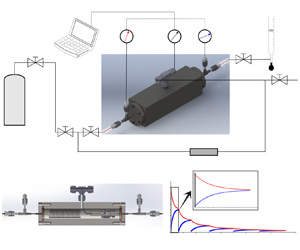
To validate the analytical solution, we build up an experimental platform as shown in figure 2. The platform can switch between pulse-decay and steady-state measurements. The steady-state measurements are used as a benchmark for the transient solution. The testing gas is nitrogen. The porous samples are polymer material and are made into cylinders with $R=1.10$ and $L=6.50$ mm. The sample is put into a metal nut and the whole nut is put into the confining chamber as shown in figure 2.

Figure 2. The diagram of experimental set-up. The confining chamber is made by mechanical finishing. The volumes of upstream and downstream chambers are 1428.68 and 1498.80 mm$^3$ respectively. The set-up can switch between the transient and steady-state measurements.

The pressure evolution data of transient measurements for one sample is shown in figure 3(a). The downstream pressure is kept at atmospheric pressure, and the upstream pressure is raised to different values. Once released, the downstream pressure rises up while the upstream pressure goes down until equilibrium is reached. Six sets of pressure data are used to calculate the permeability by our inertial solution. The full range of pressure evolution is presented in figure 3(a) to indicate no gas leakage in the measurements. Only the very beginning of the range is used to calculate permeability based on (2.29). Figure 3(b) shows the permeability under different initial pressures over the values of ${R^2 \Delta P(0)}/(\bar {\mu } \bar {\nu })$, where the intrinsic permeability, ${R^2 \Delta P(0)}/(\bar {\mu } \bar {\nu }) = 1$, can be calculated by a cubic spline interpolation. The steady-state measurements for the same sample are also performed for validation. In our experimental system, the steady-state measurements can be conducted by maintaining the upstream and downstream pressures with a low-pressure difference at one measurement. Different mean pressures are used to eliminate the slippage effect by adopting the Klinkenberg plot (Klinkenberg 1941) as figure 3(c) shows. The extrapolated intercept of the best-fit straight line represents the intrinsic permeability by the steady-state measurements.

Figure 3. Typical measurement data: (a) pressure evolutions in a pulse-decay measurement. Six sets of data are obtained by changing the initial upstream pressure. (b) Interpolation for the intrinsic permeability $\kappa _{iner}$ based on (2.29) for the pulse-decay measurements. (c) Extrapolation for intrinsic permeability $\kappa _{in}$ in the Klinkenberg plot for the steady-state measurements.

The comparisons between the high-pressure-difference transient measurements and the steady-state measurements are shown in figure 4. Each point represents a data pair $(\kappa _{in}, \kappa _{iner})$. A $45^\circ$ line is plotted and all the data points lie very near to this line, which shows clearly the consistency between these two measurements.The maximum relative difference between $\kappa _{in}$ and $\kappa _{iner}$ is 29.05 % at $\kappa _{in}=48.2$ nD $(10^{-21}\,{\rm m}^2)$. This verifies the correctness of our analytical solution for the high-pressure-difference pulse-decay method. Besides, the high-pressure difference also benefits us with a much shorter time for measurements and higher accuracy. For our measurements with a permeability at 10 nD, the measurement time is no more than 10 minutes. For a platform fabricated by classical mechanical finishing, the accuracy can reach 0.1 nD, which is two orders of magnitude lower than that of cutting-edge commercial ones. Precise machining or microfabrication techniques may further improve the accuracy.

Figure 4. The comparison between the permeability measurements by the high-pressure-difference pulse-decay method and the steady-state method. Each point was obtained by the procedure described in figure 3. The dashed line is the $45^\circ$ line.

4. Conclusions

This work presents a theoretical asymptotic solution for high-speed transient flow through microporous media by addressing the inertia effect as well as the compressibility effect and the slippage effect in the high-pressure-difference pulse-decay process. An experimental platform was designed and built to measure the permeability of tight porous materials by both transient and steady-state methods to validate the theoretical solution. The good agreements indicate that the present theoretical solution can accurately capture the inertia effect in the high-pressure-difference pulse-decay process, which can significantly shorten the time for measurements for ultra-low-permeability samples.