On the wall-bounded model of fingering double diffusive convection

Abstract

The present work aims at clarifying the effects of a solid boundary on the salt fingers in the wall-bounded double diffusive convection turbulence driven by the salinity and temperature differences between the top and bottom plates. The fluid properties are the same as the seawater, and two-dimensional direct numerical simulations are conducted over a wide range of the thermal and salinity Rayleigh numbers which measure the strength of driving salinity difference and stabilising temperature difference. We find that the bulk density ratio $\varLambda _b$, defined by the mean temperature and salinity gradients at the bulk, controls the flow morphology. As $\varLambda _b$ exceeds unity, the bulk flow shifts from wide convection rolls to slender salt fingers. Two different regimes are further identified for the cases of salt-finger type. One is the confined salt-finger regime where the characteristic height of salt fingers is comparable to the bulk height and the influences of the solid boundary are noticeable. The other is the free salt-finger regime where the salt fingers are much shorter than the bulk height. In this latter regime, the transport properties versus $\varLambda _b$ are in quantitative agreement with those obtained in the fully periodic domain (e.g. Traxler et al., J. Fluid Mech., vol. 677, 2011, pp. 530–553). For a limited range of density ratio at the highest salinity Rayleigh number considered here, multiple states can be obtained from different initial conditions. The large-scale secondary instability and spontaneous formation of staircase from finger layers are not observed in the current study.

1. Introduction

When fluid density depends on two scalar components with different molecular diffusivities, double diffusive convection (DDC) may occur if the stratifications of scalar components are in a suitable configuration. In the ocean, DDC is omnipresent as the vertical gradients of temperature and salinity favour DDC instability in many regions (You 2002). Note that temperature diffuses about 100 times faster than salt, and very rich dynamics can be excited due to this huge difference in diffusivity. Two different types of DDC are usually found in different regions. In the polar region, cold fresh water lies above warm salty water in the upper layer, and DDC occurs in the diffusive type (Kelley et al. 2003). In the (sub)tropical ocean, both temperature and salinity usually decrease with depth in the upper water, where DDC happens mainly in the fingering regime (Schmitt 1994). In fingering DDC (FDDC) the salinity gradient drives the fluid motion, while the temperature gradient stabilises the flow. FDDC can develop when the overall density is stably stratified (Stern 1960) and plays an important and unique role in oceanic mixing. For instance, FDDC can generate enhanced diapycnal mixing (Schmitt et al. 2005), and may attenuate the effects of climate change on large-scale temperature and salinity distributions in the ocean (Johnson & Kearney 2009).

Numerous efforts have been undertaken to understand the physical mechanisms and transport properties of FDDC. Reviews of early observations, experiments, simulations and theoretical models can be found in Schmitt (2003), Yoshida & Nagashima (2003), Kunze (2003) and the book of Radko (2013). Since FDDC represents a small-scale phenomenon in the ocean, it is challenging to obtain detailed information of the momentum and scalar fields in field measurements. Nonetheless, field observation has been rapidly advanced, revealing the important role of FDDC in various oceanic regions (e.g. Schmitt et al. 2005; Buffett et al. 2017; Sun, Yang & Tian 2018; Durante et al. 2019; Ashin et al. 2022). Experiments are also challenging in the sense that two scalar components must be controlled and measured simultaneously. For the convenience of experimental set-up, different scalar combinations have been employed in past other than the heat–salt system (Huppert & Turner 1981; Taylor & Bucens 1989), such as the heat–sugar system (Linden 1973), the salt–sugar system (Linden 1978; Radko & Stern 2000; Krishnamurti 2003) and the heat–copper-ion system (Hage & Tilgner 2010; Kellner & Tilgner 2014), to name a few. For these different combinations, the ratio of the molecular diffusivity of fast diffusing component to that of slow diffusing component can range from approximately 3 for the salt–sugar system to about 300 for the heat–sugar system. And experimental measurements of the instantaneous scalar fields are relatively rare.

In numerical simulations, though, it is highly convenient to precisely control flow conditions and obtain comprehensive information of the flow fields. One major difficulty in simulations is how to deal with the very small molecular diffusivity of salinity, which is typically three orders of magnitude smaller than viscosity. Scalar with small diffusivity requires very fine resolution to be fully resolved. In many numerical studies, therefore, salinity is replaced by a scalar with larger diffusivity. A frequent choice is to keep using heat as the fast diffusing component and reduce the ratio of molecular diffusivity to 3 which is similar to the salt-sugar system used in experiments (see, for example, Stellmach et al. 2011; Paparella & von Hardenberg 2012). Another technique is the multiple-resolution method as developed in our previous work (Ostilla-Mónico et al. 2015), in which salinity is solved on a refined mesh. With the help of this efficient method, very large Rayleigh numbers have been achieved for the same fluid properties as seawater in fully three-dimensional (3D) simulations (Yang, Verzicco & Lohse 2016b).

Different configurations of flow domains have been employed in existing numerical investigations of FDDC. One type is the so-called ‘run-down’ configuration, in which two homogeneous layers are separated by an interface (Sreenivas, Singh & Srinivasan 2009), and the system is isolated without any heat or salt exchange with the outside. The top layer has both higher temperature and salinity so that salt fingers develop around the initial interface. This configuration is identical to many early experimental set-up, such as Turner (1967), Linden (1973) and Schmitt (1979). Since the total potential energy is fixed by the initial field, the system undergoes continuous transition until the available energy is completely consumed, i.e.the flow cannot reach a statistically steady state.

In order to maintain a statistically steady state, a constant driving force should be introduced. Two typical choices have been utilised. The first employs constant background temperature and salinity gradients and simulates the temperature and salinity deviated from this background field. Then, a fully periodic domain can be used, and the flow quantities can be numerically solved efficiently by using the standard pseudo-spectral scheme (Stellmach et al. 2011; Traxler et al. 2011). Another choice is the wall-bounded model, which is commonly used in thermal convection (Ahlers, Grossmann & Lohse 2009). In this configuration, a fluid layer is bounded from top and bottom by two parallel plates which usually have constant temperature and salinity. Therefore, constant differences in temperature and salinity are maintained across the layer. Wall-bounded FDDC has been investigated in both experiments and numerical simulations (Radko & Stern 2000; Krishnamurti 2003; Hage & Tilgner 2010; Kellner & Tilgner 2014; Yang et al. 2015, 2016b; Rosenthal, Lüdemann & Tilgner 2022).

One inevitable question about the wall-bounded FDDC model is the influence of the solid plates which are not present in the oceanic FDDC. The free-slip condition can be used to eliminate the viscous drag along the two plates, but the effects of non-penetration condition still exist. Our previous study indeed shows that wall-bounded FDDC with free-slip and no-slip boundary conditions exhibit very similar behaviours in flow structures and transport properties (Yang, Verzicco & Lohse 2016c). In the triply periodic domain, the domain size needs to be large enough to remove the numerical constraints on finger length scales (Traxler et al. 2011). However, if the domain is too large, secondary large-scale instabilities can develop and drive the system away from pure finger state to staircase state (Radko 2003; Stellmach et al. 2011). In the wall-bounded domain, multiple final statistically steady states, including pure finger state and staircases with different layer configurations, can be established for the exact same control parameters, i.e.the salinity Rayleigh number and the density ratio (defined as the ratio between the density change caused by temperature difference and that caused by salinity difference) (Yang et al. 2020). Therefore, both the fully periodic model and the wall-bounded model have provided valuable insights into the dynamics and evolution of fully developed FDDC staircases. It is also worth mentioning that the so-called ‘elevator modes’ which grow exponentially in the triply periodic Rayleigh–Bénard (RB) convection (Calzavarini et al. 2006) are exactly the tall-finger modes in triply periodic FDDC (Schmitt 1979; Radko 2013). Apparently, such elevator modes are prevented by the two solid plates in wall-bounded FDDC.

Nevertheless, in the wall-bounded FDDC model, boundary layers always develop adjacent to the two plates in the momentum, temperature and salinity fields. The appearance of boundary layers and their interaction with the salt fingers in the bulk usually affect the flow dynamics and transport behaviours (Radko & Stern 2000; Yang et al. 2016b). One of the most direct impacts is that the density ratio measured away from the boundary layers differs greatly from the value set by the scalar differences between the two plates. Theoretically, salt fingers only occur when the density ratio is greater than 1, but previous wall-bounded experiments and numerical simulations have found that the flow morphology can shift from wide convection rolls to slender salt fingers when the density ratio is less than 1 (Hage & Tilgner 2010; Kellner & Tilgner 2014; Yang, Verzicco & Lohse 2016a). The contradiction here comes from the fact that the parameter that actually controls the salt-finger behaviours should be the density ratio defined in the bulk area rather than the density ratio between the two plates. Our recent work (Yang et al. 2020) indeed discovered that, for fingering layers which either are parts of staircases or occupy the whole bulk, their heat and salinity fluxes and the flux ratio are very similar to those measured from salt fingers in fully periodic domains (Stellmach et al. 2011) if all parameters are defined by the local scalar gradients of finger layers.

Therefore, this paper aims to thoroughly investigate the dependence of salt-finger behaviours on the density ratio measured in the bulk area, and clarify the parameter range where transport behaviours are determined intrinsically by salt fingers and independent of boundary. To achieve these, we conduct systematic simulations of FDDC using fluid properties identical to those of seawater. We define the bulk density ratio by the temperature and salinity gradients measured away from the boundary layers and examine its relationship with the characteristic length scales and vertical transport properties. Furthermore, to fully understand the influences of solid boundary on FDDC, we investigate the flow evolution together with the final possible multilayer states.

The rest of paper is organised as follows. The governing equations and numerical methods are detailed in § 2. The flow evolution is discussed in § 3. The characteristic length scales and the transport properties are discussed in §§ 4 and 5, respectively. The conclusions are given in § 6.

2. Governing equations and numerical methods

We first introduce the dimensional governing equations for FDDC, which take the same form in each model. We employ a linear equation of state as $\rho ^*=\rho ^*_0(1-\beta _T \theta ^* +\beta _S s^*)$. Here $\rho ^*$ is density, with the subscript ‘0’ denoting the value at the reference state, $\theta ^*$ and $s^*$ are the temperature and salinity with respect to the corresponding reference values, $\beta _T$ is the thermal expansion coefficient and $\beta _S$ is the coefficient of haline contraction, respectively. Hereafter, the asterisk denotes the dimensional quantity. Then, under the Oberbeck–Boussinesq approximation, the governing equations read

(2.1a)$$\begin{gather} \partial_t \boldsymbol{u}^* + \boldsymbol{u}^*\boldsymbol{\cdot}\boldsymbol{\nabla}\boldsymbol{u}^* ={-}\boldsymbol{\nabla} p^* + \nu {\nabla}^2\boldsymbol{u}^* + g(\beta_T \theta^* - \beta_S s^*)\boldsymbol{e}_z, \end{gather}$$

(2.1b)$$\begin{gather}\partial_t \theta^* + \boldsymbol{u}^*\boldsymbol{\cdot}\boldsymbol{\nabla} \theta^* = \kappa_T \nabla^2\theta^*, \end{gather}$$

(2.1c)$$\begin{gather}\partial_t s^* + \boldsymbol{u}^*\boldsymbol{\cdot}\boldsymbol{\nabla} s^* = \kappa_S \nabla^2 s^*, \end{gather}$$

(2.1d)$$\begin{gather}\boldsymbol{\nabla}\boldsymbol{\cdot}\boldsymbol{u}^* = 0. \end{gather}$$

Here, $\boldsymbol {u^*}$ is velocity, $p^*$ is pressure, $g$ is the gravitational acceleration, $\boldsymbol {e}_z$ is the unit vector in the vertical $z$ direction, $\nu$ is viscosity and $\kappa$ is molecular diffusivity, respectively. Note that density has been absorbed into pressure.

2.1. Wall-bounded model

In the wall-bounded model, we consider a fluid layer bounded by two parallel plates from top and bottom. The two plates are perpendicular to the gravity and separated by a height $H$, which are set as non-slip walls with constant temperature and salinity. The top plate has higher temperature and salinity so that the system is in the FDDC regime. In the horizontal directions, periodic boundary conditions are applied. The boundary conditions then read

(2.2a)$$\begin{gather} \boldsymbol{u}^*=\boldsymbol{0},\ s^*=\varDelta_S,\ \theta^*=\varDelta_T, \quad \mbox{at}\ z^*/H=1, \end{gather}$$

(2.2b)$$\begin{gather}\boldsymbol{u}^*=\boldsymbol{0},\ s^*=0,\ \theta^*=0, \quad \mbox{at}\ z^*/H=0. \end{gather}$$

Here the fluid at bottom plate is chosen as the reference state, and $\varDelta _T$ and $\varDelta _S$ are the constant temperature and salinity differences between the two plates, respectively.

The governing equations (2.1) are then non-dimensionalised by the height $H$, the constant temperature and salinity differences $\varDelta _T$ and $\varDelta _S$ between the two plates and the free-fall velocity $\sqrt {gH\beta _S\varDelta _S}$, respectively. The control parameters include the Prandtl number, the Schmidt number and two Rayleigh numbers, which are defined respectively as

(2.3a–d)\begin{equation} {\textit{Pr}} = \frac{\nu}{\kappa_T}, \quad {\textit{Sc}} = \frac{\nu}{\kappa_S}, \quad {\textit{Ra}}_T = \frac{g\beta_T\varDelta_T H^3}{\nu\kappa_T}, \quad {\textit{Ra}}_S = \frac{g\beta_S\varDelta_S H^3}{\nu\kappa_S}. \end{equation}

Throughout this study, we fix ${\textit {Pr}}=7$ and ${\textit {Sc}}=700$, which are the typical values for temperature and salinity in the ocean. The Lewis number, i.e. the ratio between the two diffusivities, is then ${\textit {Le}}={\textit {Sc}}/{\textit {Pr}}=100$. The relative strength of the temperature difference to the salinity difference can be measured by the density ratio as

(2.4)\begin{equation} \varLambda = \frac{\beta_T\,\varDelta_T}{\beta_S\,\varDelta_S} = \frac{{\textit{Sc}}\,{\textit{Ra}}_T}{{\textit{Pr}}\,{\textit{Ra}}_S} = \frac{{\textit{Le}}\,{\textit{Ra}}_T}{{\textit{Ra}}_S}. \end{equation}

Then the non-dimensional governing equations are

(2.5a)$$\begin{gather} \partial_t \boldsymbol{u} + \boldsymbol{u}\boldsymbol{\cdot}\boldsymbol{\nabla}\boldsymbol{u} ={-}\boldsymbol{\nabla} p + {\textit{Sc}}^{1/2}{\textit{Ra}}^{{-}1/2}_S\,{\nabla}^2\boldsymbol{u} + (\varLambda \theta - s)\boldsymbol{e}_z, \end{gather}$$

(2.5b)$$\begin{gather}\partial_t \theta + \boldsymbol{u}\boldsymbol{\cdot}\boldsymbol{\nabla} \theta = Sc^{1/2}{\textit{Ra}}_S^{{-}1/2}{\textit{Pr}}^{{-}1}\,\nabla^2\theta, \end{gather}$$

(2.5c)$$\begin{gather}\partial_t s + \boldsymbol{u}\boldsymbol{\cdot}\boldsymbol{\nabla} s = {\textit{Sc}}^{{-}1/2}{\textit{Ra}}_S^{{-}1/2}\,\nabla^2 s, \end{gather}$$

(2.5d)$$\begin{gather}\boldsymbol{\nabla}\boldsymbol{\cdot}\boldsymbol{u} = 0, \end{gather}$$

with the boundary conditions

(2.6a)$$\begin{gather} \boldsymbol{u}=\boldsymbol{0},\ s=1,\ \theta=1, \quad \mbox{at}\ z=1, \end{gather}$$

(2.6b)$$\begin{gather}\boldsymbol{u}=\boldsymbol{0},\ s=0,\ \theta=0, \quad \mbox{at}\ z=0. \end{gather}$$

2.2. Fully periodic model

In the fully periodic model, periodic boundary conditions are applied in both vertical and horizontal directions. Constant salinity and temperature gradients are sustained as the background state and drive the flow. The scalar fields are separated as

(2.7a,b)\begin{equation} s^*=\bar{S}^*_zz^*+s^{\prime *}, \quad \theta^*=\bar{T}^*_zz^*+\theta^{\prime *}. \end{equation}

Here, $\bar {S}^*_z$ and $\bar {T}^*_z$ are the constant vertical gradients of salinity and temperature, and $s^{\prime *}$ and $\theta ^{\prime *}$ are the deviations from the background state, respectively. For the velocity field, the background state is set to zero, i.e. $\boldsymbol {u'}=\boldsymbol {u}$. Usually in the fully periodic model the expected finger scale is used as the characteristic length scale, which is defined as (Stern 1960)

(2.8)\begin{equation} d=\left(\frac{\kappa_T \nu}{g\beta_T \bar{T}^*_z}\right)^{1/4}. \end{equation}

The corresponding time scale is $d^2/\kappa _T$, and the salinity and temperature scales are defined as $(\beta _T/\beta _S)\bar {T}^*_zd$ and $\bar {T}^*_zd$, respectively. Then the non-dimensional governing equations read

(2.9a)$$\begin{gather} \partial_t \boldsymbol{u} + \boldsymbol{u}\boldsymbol{\cdot}\boldsymbol{\nabla}\boldsymbol{u} = {\textit{Pr}}( -\boldsymbol{\nabla} p' +{\nabla}^2\boldsymbol{u} + (\theta' - s')\boldsymbol{e}_z), \end{gather}$$

(2.9b)$$\begin{gather}\partial_t \theta' + \boldsymbol{u}\boldsymbol{\cdot}\boldsymbol{\nabla} \theta'={-}w+\nabla^2\theta', \end{gather}$$

(2.9c)$$\begin{gather}\partial_t s' + \boldsymbol{u}\boldsymbol{\cdot}\boldsymbol{\nabla} s'={-}\frac{w}{\bar{\varLambda}} +\frac{1}{{\textit{Le}}}\nabla^2 s', \end{gather}$$

(2.9d)$$\begin{gather}\boldsymbol{\nabla}\boldsymbol{\cdot}\boldsymbol{u} = 0. \end{gather}$$

Here $p'$ is the pressure deviation with respect to the hydrostatic equilibrium, and $w$ is the vertical velocity. The constant background density ratio $\bar {\varLambda }$ is defined as

(2.10)\begin{equation} \bar{\varLambda}=\frac{\beta_T \bar{T}^*_z}{\beta_S \bar{S}^*_z}. \end{equation}

Note that $\bar {\varLambda }$ is constant over the entire domain and does not change during simulations for the fully periodic model. In wall-bounded model, $\varLambda$ represents the total density ratio between the two plates. Hereafter, we refer to the control parameters of the wall-bounded model as the global parameters to distinguish them from the local ones measured at different heights.

2.3. Numerical method

Direct numerical simulations (DNS) are conducted for FDDC with the wall-bounded model. For comparison, the theoretical and numerical results of the fully periodic model are directly adopted from previous works including Schmitt (1979), Traxler et al. (2011) and Stellmach et al. (2011). The non-dimensional governing equations (2.5) are numerically solved by using our in-house code, which employs a finite-difference scheme and a fractional time-step method (Ostilla-Mónico et al. 2015). In particular, the code utilises a dual-resolution technique to deal with the salinity field which has a very high Schmidt number. A base mesh is used for the momentum and temperature fields, while a refined mesh for the salinity field. For example, when the refinement factors are two in both the horizontal and vertical directions, there are four mesh cells for the salinity field in one base cell for the temperature or velocity fields. A local mass-conserved interpolation method is developed to interpolate the velocity field from the base mesh to the refined mesh. The code has been applied extensively to FDDC in our previous works (Yang et al. 2015, 2016b,c), and validated by one-to-one comparisons with experiments (Yang et al. 2015). Still, fully 3D DNS with ${\textit {Pr}}=7$ and ${\textit {Sc}}=700$ are very challenging for a systematic study. Here we confine ourselves to two-dimensional (2D) simulations and explore a wide range of the salinity Rayleigh number and the density ratio (see the Appendix).

It is important to note that the transport efficiency is different for 2D and 3D salt fingers due to the different shapes of horizontal cross sections. The 3D fingers usually have circular cross section, whereas the 2D fingers are planar and have infinite length in the third directions. At $\varLambda =2$, the 3D heat and salinity fluxes are approximately twice of those in 2D cases (Stern, Radko & Simeonov 2001). Nevertheless, when all the fluxes are normalised by the values of the case with smallest $\varLambda$ considered in this study, their overall trends versus $\varLambda$ are quite similar to our previous 3D simulations (Yang et al. 2016a) at small ${\textit {Ra}}_S$ (see figure 11). Therefore, we believe that 2D simulations can still provide valuable insights into the physics of FDDC. Another concern about 2D simulations is the zonal flow characterised by the horizontal shear layers, which does not exist in 3D cases (Van Der Poel et al. 2014). It usually happens at small ${\textit {Pr}}$ and small aspect ratio. In the current work, once the zonal flow is observed, we increase the domain width and rerun the case. For all the simulations considered here, the shear layers or the zonal flow do not emerge during the final statistically steady stage.

In the wall-bounded model, the flow morphology can shift from wide convection rolls to slender fingers (Kellner & Tilgner 2014; Yang et al. 2016a; Rosenthal et al. 2022) for different parameters. In order to consistently investigate the flow morphology, the salinity Rayleigh number ${\textit {Ra}}_S$, which measures the strength of driving force, is chosen as one primary global control parameter. We simulate 5 different salinity Rayleigh numbers over 4 decades from $10^{8}$ to $10^{12}$. The global density ratio $\varLambda$ is then systematically changed for each ${\textit {Ra}}_S$. For the 4 lower Rayleigh numbers $\varLambda$ increases from $0.001$ up to $30$. For the highest $Ra_S=10^{12}$, the smallest density ratio is set as $0.003$ due to computational resource constraints. Note that we choose $\varLambda$ starting at a value well below unity, since salt fingers can develop in the bulk of wall-bounded domain even when the overall density is unstably stratified (Hage & Tilgner 2010; Schmitt 2011), and the transition from wide convection rolls to slender salt fingers happens at strongly unstable density stratification (Kellner & Tilgner 2014; Yang et al. 2016a). The details about numerics and the global responses are summarised in the Appendix.

Since the global density ratio $\varLambda$ cannot properly characterise the bulk flow structures in the wall-bounded domain, it is convenient to redefine the density ratio using the bulk quantities when the flow reaches a fully developed state. Similar to the fully periodic model, we measure the central vertical gradients of the temperature and salinity profiles for all cases, which are denoted by $T_z$ and $S_z$, respectively. Specifically, the slopes are calculated from the mean profiles $\langle \theta \rangle _h$ and $\langle s\rangle _h$ by a linear fitting over the range $0.25\leqslant z \leqslant 0.75$. Hereafter, the bracket $\langle {\cdot } \rangle _h$ stands for the spatial average in the horizontal direction. Then the bulk density ratio can be calculated as

(2.11)\begin{equation} \varLambda_b=\frac{\beta_T T^*_z}{\beta_S S^*_z}=\varLambda\frac{T_z}{S_z}, \end{equation}

where $T^*_z$ and $S^*_z$ represent the dimensional forms of $T_z$ and $S_z$, respectively. Figure 1 displays the variation of the mean bulk density ratio $\bar {\varLambda }_b$ versus the global density ratio $\varLambda$. The overline denotes the temporal average. The error bars of $\bar {\varLambda }_b$ are also plotted. Hereafter, the error bars are calculated by the standard deviations of the time history. In the logarithmic coordinate, the error bars which extend to the negative values are not displayed. In general, $\bar {\varLambda }_b$ increases from values very close to zero to around $53$ as $\varLambda$ changes from $0.001$ to $30$. Negative $\bar {\varLambda }_b$ appears in some cases with small $\varLambda$, which are not shown in the figure. The error bars are large for small $\varLambda$, since $S_z$ oscillates severely around zero which is caused by large convection rolls. As $\varLambda$ becomes larger, the wide convection rolls are gradually replaced by slender salt fingers which generate more stable and positive $S_z$, and the uncertainty of $\varLambda _b$ reduces. In the ocean, the observed strong FDDC often has a density ratio of $1<\bar {\varLambda }_b<2$ (Schmitt et al. 2005; Durante et al. 2019), which corresponds to a narrow range of $\varLambda$ as shown in figure 1(b).

Figure 1. The mean bulk density ratio $\bar {\varLambda }_b$ versus the global density ratio $\varLambda$. (a) The whole dataset with error bars except for the cases with negative $\bar {\varLambda }_b$. Some halves of error bars that extend to negative values are not displayed either. (b) Enlarged view of the plot highlighting the cases with $\bar {\varLambda }_b\in [1,10]$.

3. On the flow evolution

We first discuss the choice of initial conditions and the temporal evolution of the flow fields. For all cases, the fluid is stationary at the beginning. For the simulations with ${\textit {Ra}}_S\leqslant 10^{11}$, initially the temperature field is a linear distribution between the two plates, while the salinity field is uniform and equals to the mean of the values at two plates, respectively. Small perturbations are added to trigger the flow motions. These initial conditions are the same as those in the experiments of Hage & Tilgner (2010) and our previous simulations (Yang et al. 2015, 2016b). For the cases with ${\textit {Ra}}_S=10^{12}$, to save computing time, the initial fields are directly set as one set of fully developed fields from the previous case with smaller $\varLambda$. Our previous work (Yang et al. 2020) reveals that for fixed ${\textit {Le}}=3$ and $\varLambda =1.2$, multiple equilibrium staircase states can be established from different initial distributions for the same global control parameters when ${\textit {Ra}}_S$ is above certain critical value. Here we first present the evolution of the salt fingers in the wall-bounded model with ${\textit {Le}}=100$, and demonstrate that the initial conditions do not influence the final state for the cases with ${\textit {Ra}}_S\leqslant 10^{11}$, but the multiple multilayer states emerge from different initial conditions for ${\textit {Ra}}_S=10^{12}$.

3.1. The single final state for ${\textit {Ra}}_S\leq 10^{11}$

An additional case is run for ${\textit {Ra}}_S=10^{10}$ and $\varLambda =0.1$, and initially both scalars have a vertically linear distribution, which we refer to as the linear initial condition. That with linear temperature distribution and uniform salinity distribution is referred to as the mixed initial condition. Figure 2 plots the time history of bulk density ratio $\varLambda _b$ and Reynolds number $Re$ for the two cases with mixed and linear initial conditions. The Reynolds number is defined as $Re=U^*_{rms}H/\nu$, in which $U^*_{rms}$ is the dimensional root-mean-square (r.m.s.) value of the velocity magnitude computed over the entire domain. We also show the temporal evolution of the scalar profiles in figure 3. For the case with the mixed initial condition, $\varLambda _b$ is very large in the bulk at the beginning since $S_z$ is close to zero. As plumes grow from the top and bottom boundaries where the salinity field is strongly unstable, $Re$ increases rapidly and $\varLambda _b$ decreases towards the values of final statistically steady state. Figures 3(a) and 3(b) indicate that nearly linear profiles directly build up in the bulk as buoyancy-driven motions develop with time.

Figure 2. Comparison of the temporal evolution of (a) bulk density ratio and (b) Reynolds number for the two cases starting from the mixed initial condition (blue dashed lines) and the linear initial condition (red solid lines). The global control parameters are $Ra_S=10^{10}$ and $\varLambda =0.1$.

Figure 3. Temporal evolution of the horizontally averaged scalar profiles starting from different initial conditions for ${\textit {Ra}}_S=10^{10}$ and $\varLambda =0.1$. Panels (a,b) show the salinity and temperature profiles for the case with mixed initial condition, respectively. Panels (c,d) show the same quantities for the case with linear initial condition.

The case with the linear initial condition exhibits a completely different initial development. With $\varLambda =0.1$, the density field is unstably stratified over the entire domain at the beginning, which results in complete overturn with respect to the middle height and induces a sharp increase in $Re$, see figure 2(b). The overturn can be seen at the left part of figure 3(c) where the heavy fluid with high salinity and the light fluid with low salinity accumulate near the bottom and top boundaries, respectively. The bulk temperature then homogenises faster than salinity due to larger diffusivity. During this stage the bulk density ratio remains nearly zero due to the small value of $T_z$, as shown in figure 2(a). As plumes emanate from both plates and transport heat and salinity into the bulk, linear mean profiles with upward gradients are gradually established, which is accompanied by the change of $\varLambda _b$ from negative to positive values at approximately $t=380$ in figure 2(a).

Despite the different initial conditions, both cases evolve towards the same final state roughly after $t=500$ with exactly the same $\varLambda _b$ and $Re$, as indicated by figures 2 and 3. For the case with mixed initial condition, salt fingers first grow from the boundary and extend to the bulk. In contrast, for the case with linear initial condition, fingers also directly emerge at the bulk after the overturn of whole fluid layer. Eventually the salt fingers occupy the whole bulk at the final state. It is then very likely that a complete fingering bulk will be obtained regardless of the initial distribution, and the same final state can be achieved.

3.2. The possible multilayer states at ${\textit {Ra}}_S=10^{12}$

At ${\textit {Ra}}_S=10^{12}$, even 2D simulations are rather expensive. Therefore, for the cases with the same domain width, the simulation is first run at smaller density ratio until the flow reaches the statistically steady state. Then, an instantaneous flow field is used as the initial field for the next simulation with a larger density ratio. For $\varLambda \leq 0.2$, the bulk consists of large convection rolls. 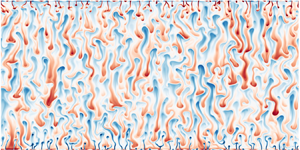A transition in flow morphology is observed over the $0.2<\varLambda <0.3$, which is illustrated in figure 4 by the instantaneous vertical velocity fields of four cases with gradually increasing density ratio. As $\varLambda$ increases from $0.20$ to $0.27$, the characteristic width of the flow structures in the bulk decreases as the wide convection rolls in figures 4(a) and 4(b) are replaced by slender finger-like structures in figures 4(c) and 4(d). Meanwhile, the plumes originated from two plates extend deeper into the bulk. Note that at $\varLambda =0.25$ the slender finger structures in the bulk have different width compared with the slender plumes near the top and bottom boundaries. This difference is weaker at $\varLambda =0.27$. The transition of the bulk structures and the extension of the boundary plume regions can be also seen in the variation of mean salinity profiles which are shown in figure 5(a). As $\varLambda$ increases, a linear segment first appears near the boundary in the profile while at the bulk $\langle \bar {s} \rangle _h$ is still very close to $0.5$. This corresponds to the roll-like bulk with extending plume regions near the boundary. As $\varLambda$ further increases, the profile becomes linear over the entire bulk and finger structures dominate.

Figure 4. The flow morphology depicted by the contours of vertical velocity for four cases with fixed ${\textit {Ra}}_S=10^{12}$ and (a) $\varLambda =0.20$, (b) $\varLambda = 0.23$, (c) $\varLambda = 0.25$ and (d) $\varLambda = 0.27$, respectively. The initial condition is the fully developed flow field at smaller $\varLambda$.

Figure 5. (a) The time-averaged salinity vertical profiles for all the cases with ${\textit {Ra}}_S=10^{12}$, coloured by the global density ratio $\varLambda$. The dashed lines mark the four cases with $\varLambda =0.20, 0.23, 0.25$ and $0.27$ which are shown in figure 4. (b) The instantaneous salinity vertical profiles for the case with ${\textit {Ra}}_S=10^{12}$ and $\varLambda =0.23$ at different times. The colour bar is determined by the simulation time $t$. In order to clearly demonstrate the transition and due to the symmetry about $z=0.5$, only the region with $0.5\leqslant z \leqslant 1$ and $0.5\leqslant \langle s \rangle _h \leqslant 0.56$ is shown.

The above observations indicate that during the transition from the roll-type bulk to the finger-type one, multilayer structures with different characteristic widths may appear, which resemble the thermohaline staircases (see, e.g., figure 1A of Schmitt et al. 2005). The four cases with $\varLambda =0.22$, $0.23$, $0.24$ and $0.25$ are also run with the mixed initial condition, and indeed different final states are obtained. The evolution of flow morphology is very similar for these four cases, and figure 6 only shows the temporal evolution of the case with $\varLambda =0.23$ and starting from the mixed initial condition. At the final state, the bulk consists of slender fingers, which is totally different from the state shown in figure 4(b) with the same global parameters. More interestingly, the characteristic width is smaller at the middle part of the bulk and larger at the two sides. Linear segments with different slopes develop in the mean salinity profiles, as shown in figure 5(b). The middle part with thinner fingers has a larger slope compared with that of the two regions with thicker fingers. Comparing figures 5(a) and 5(b), such different final states strongly suggest the existence of multiple equilibrium states based on our previous study at ${\textit {Le}}=3$ (Yang et al. 2020).

Figure 6. The flow morphology depicted by the contours of vertical velocity for the case with ${\textit {Ra}}_S=10^{12}$ and $\varLambda = 0.23$ at four different simulation times: (a) $t=40$, (b) $t=200$, (c) $t=400$ and (d) $t=3000$. The mixed initial condition is applied.

It should be pointed out that the multilayer state obtained here is the result of flow evolution from the specific initial field, but not from the secondary instability of finger layers which appears in the periodic domain (Stellmach et al. 2011). In addition, once the whole bulk is occupied by salt fingers with uniform characteristic width, the final state is unlikely to be affected by the initial conditions. A thorough investigation of multiple equilibrium states requires more simulations at the relevant parameter range or at higher Rayleigh number, which is beyond the scope of the current study. In the following we focus on the salt-finger state.

4. On the length scales

We now investigate the characteristic length scales of the structures in the bulk. The horizontal width and the vertical height can be extracted by using the auto-correlation functions of the vertical velocity $w$, which are calculated as

(4.1a,b)\begin{equation} R_x(\delta x) = \frac{\langle \overline{w(x,z,t) w(x+\delta x,z,t)} \rangle_b } {\overline{\langle w^2(x,z,t)} \rangle_b}, \quad R_z(\delta z) = \frac{\langle \overline{w(x,z,t) w(x,z+\delta z,t)} \rangle_b } {\langle \overline{w^2(x,z,t)} \rangle_b}. \end{equation}

Hereafter, $\langle \rangle _b$ denotes the spatial average over the bulk region $0.25\leqslant z \leqslant 0.75$. Figure 7 demonstrates the typical behaviours of $R_x$ and $R_z$ for cases with ${\textit {Ra}}_S=10^{10}$. For all cases $R_x$ can always decrease to zero at certain horizontal distance $\delta _x$, indicating the domain width is large enough and the periodic boundary condition is adequate. For some cases with small $\varLambda$, $R_z$ remains positive for all $\delta _z$, as the large-scale convection rolls occupy the whole bulk. If the auto-correlation function decreases to zero, the location of the first zero point can be treated roughly as a quarter of the corresponding wavelength. To demonstrate this, we utilise the sinusoidal functions as model distributions, which have been used frequently in the past (see, e.g., Stern (1960) and Schmitt (1979)). Specifically, for the vertical velocity field of $w=w_0(t)\sin (({2{\rm \pi} }/{\lambda _x})x)\sin (({2{\rm \pi} }/{\lambda _z})z)$, in which $\lambda _x$ and $\lambda _z$ are the respective horizontal and vertical wavelengths, the auto-correlation functions (4.1a,b) vanish at $\delta _x=\lambda _x/4$ and $\delta _z=\lambda _z/4$, since

(4.2a)$$\begin{gather} R_x(\lambda_x/4) = \frac{\left\langle \overline{w_0^2\sin^2\left(\dfrac{2{\rm \pi}}{\lambda_z}z\right) \sin\left(\dfrac{2{\rm \pi}}{\lambda_x}x\right)\cos\left(\dfrac{2{\rm \pi}}{\lambda_x}x\right)} \right\rangle_b } {\overline{\langle w^2(x,z,t)} \rangle_b}=0, \end{gather}$$

(4.2b)$$\begin{gather}R_z(\lambda_z/4) = \frac{\left\langle \overline{w_0^2\sin^2\left(\dfrac{2{\rm \pi}}{\lambda_x}x\right) \sin\left(\dfrac{2{\rm \pi}}{\lambda_z}z\right)\cos\left(\dfrac{2{\rm \pi}}{\lambda_z}z\right)} \right\rangle_b } {\langle \overline{w^2(x,z,t)} \rangle_b}=0. \end{gather}$$

Therefore, $\lambda _x$ and $\lambda _z$ can be calculated as four times the locations of the first zero points of $R_x$ and $R_z$, respectively.

Figure 7. (a) The horizontal auto-correlation functions $R_x$ versus the horizontal separation $\delta _x$ and (b) the vertical auto-correlation functions $R_z$ versus the vertical separation $\delta _z$ for all cases with $Ra_S=10^{10}$. The colours are determined by $\varLambda$.

We first examine the horizontal wavelength $\lambda _x$. Figure 8(a) depicts the dependence of $\lambda _x$ on the mean bulk density ratio $\bar {\varLambda }_b$ for all cases with $\bar {\varLambda }_b>0$. For ${\textit {Ra}}_S\geq 10^{10}$, $\lambda _x$ is close to $2$ for $\bar {\varLambda }_b<1$. Since the aspect ratio $\varGamma$ of domain is $2$ for these cases, $\lambda _x=2$ indicates that a pair of large convection rolls dominates the bulk. At smaller ${\textit {Ra}}_S$, $\varGamma$ is larger than $2$ and several pairs of convection rolls appear, resulting in smaller $\lambda _x$ at low $\bar {\varLambda }_b$. For all ${\textit {Ra}}_S$, $\lambda _x$ starts to decrease at approximately $\bar {\varLambda }_b=1$, indicating a transition from rolls to fingers in the bulk. Before and during this transition, $\varLambda _b$ fluctuates strongly with time due to the fact that $S_z$ is close to zero, and the error bars are large as shown in figure 8(a). However, when $\bar {S}_z>0.01$, the error bars becomes very small and negligible. Consequently, we define the finger-type cases by the criteria $\bar {\varLambda }_b>1$ and $\bar {S}_z>0.01$, as indicated by the vertical and horizontal dashed lines in figure 8(a). Meanwhile, when $\lambda _x$ is normalised by the finger scale $d$, all data of salt-finger cases collapse onto a single curve, as shown in figure 8(b). The linear analysis of fully periodic model reveals that the fastest-growing wavelength ($FGW$) normalised by $d$ depends only on the background density ratio (equivalent to the bulk density ratio of wall-bounded model) for given fluid properties. This theoretical prediction (calculated by (13) of Schmitt 1979) is shown by the dashed line in figure 8(b). The numerical results of the current wall-bounded model show similar trends to those in the fully periodic model. For large $\bar {\varLambda }_b$, nonlinear results are quantitatively consistent with linear predictions. Apparent discrepancies exist when $\bar {\varLambda }_b$ is close to unity, because the salt-finger bulk is more turbulent and nonlinear effects are stronger at this regime. The fact that the finger width in fully nonlinear flow shares similar behaviour as in the linear regime has been reported by Traxler et al. (2011) in the fully periodic simulations and recently also proposed by Middleton & Taylor (2020) through an energy method.

Figure 8. (a) The horizontal wavelength $\lambda _x$ vs the mean bulk density ratio $\bar {\varLambda }_b$. The cases with negative $\bar {\varLambda }_b$ are not shown. The dashed lines characterise the salt-finger cases $(\bar {\varLambda }_b>1$ and $\bar {S}_z>0.01)$. In (b–d) only the salt-finger cases are shown. In (b), $\lambda _x$ normalised by the finger scale $d$ is plotted versus $\bar {\varLambda }_b$. The dashed line indicates the linear fastest-growing wavelength ($FGW$) normalised by $d$ (see (13) in Schmitt 1979). In (c), $\lambda _x$ is plotted versus the mean bulk Rayleigh number $\overline {Ra}_b$. In (d), $FGW$ normalised by $H$ is plotted versus $\overline {Ra}_b$ with the solid line indicating $H=25FGW$. The dashed lines in (c,d) indicate the $-1/4$ power-law scaling. The error bars of $\bar {\varLambda }_b$ and $\overline {Ra}_b$ are also displayed (halves of bars that extend to negative values are not shown).

Figure 8(b) indicates that $\lambda _x/d$ is nearly constant for $5<\bar {\varLambda }_b<50$. Recall the definition (2.8), constant $\lambda _x/d$ suggests a power-law scaling $\lambda _x\sim (\bar {T}_z)^{-1/4}$. If we define the bulk thermal Rayleigh number by using the bulk temperature gradient $T_z$ as

(4.3)\begin{equation} {\textit{Ra}}_b= \frac{g\beta_TT_z^* H^4}{\nu\kappa_T}=T_z{\textit{Ra}}_T, \end{equation}

then the scaling $\lambda _x\sim (\overline {{\textit {Ra}}}_b)^{-1/4}$ should hold for intermediate bulk density ratio $5<\bar {\varLambda }_b<50$, which can be confirmed by figure 8(c). Indeed, the $-1/4$ scaling is observed for high $\bar {\varLambda }_b$, and again the nonlinear effects attribute to the deviations for low $\bar {\varLambda }_b$. Figure 8(d) plots the dependence of $FGW/H$ on $\overline {{\textit {Ra}}}_b$, and nearly all data follow the scaling $FGW/H\sim (\overline {{\textit {Ra}}}_b)^{-1/4}$. It should be pointed out that in the periodic model large-scale secondary instabilities develop when $H\geq 25FGW$ (Stellmach et al. 2011; Traxler et al. 2011), which is indicated by the horizontal solid line in figure 8(d). Here only a few cases satisfy this criterion at large ${\textit {Ra}}_S$ and $\bar {\varLambda }_b$. Since the height of the fingering bulk is smaller than $H$, the number of cases with $H_{bulk}\geq 25FGW$ is even smaller. Therefore, in our simulations, the secondary instabilities are not observed.

We already identify the cases of finger type by $\bar {\varLambda }_b>1$ and $\bar {S}_z>0.01$. However, detailed investigations reveal that two different types of flow morphology can be further identified within the category of finger type. To demonstrate this, we calculate the joint probability density functions (p.d.f.s) of $w'$ and $s'$ sampled in the region $0.25\leqslant z \leqslant 0.75$ for three cases with ${\textit {Ra}}_S=10^{10}$ and $\varLambda =0.01, 0.1, 1$. The corresponding values of $\bar {\varLambda }_b$ are 0.18, 2.16 and 10.1, respectively. These joint p.d.f.s are displayed in figure 9. When $\varLambda =0.01$, the p.d.f. has a peak ridge along the axis $s'=0$ and over a wide range of $w'$. This region corresponds to low salinity anomaly with very different vertical velocity. There are also occasions with large positive (negative) salinity anomaly $s'$ associated with large negative (positive) vertical velocity $w'$, but the p.d.f. is much lower. All these behaviours of p.d.f. distribution in figure 9(a) are consistent with the large convection rolls at $\varLambda =0.01$, which are mainly driven by the plumes growing from the boundary, instead of the local salinity anomaly in the bulk. In contrast, when $\varLambda =1$ and the bulk is dominated by slender salt fingers, the joint p.d.f. is basically along the straight line of $w'/w'_{max}=-s'/s'_{max}$, as shown in figure 9(c). The strong anti-correlation between $w'$ and $s'$ implies that the vertical velocity is mainly driven by the local salinity anomaly in the bulk which is carried by salt fingers.

Figure 9. Joint probability of the vertical velocity anomaly and the salinity anomaly normalised by their maximum values, respectively. The control parameters read ${\textit {Ra}}_S=10^{10}$ and (a) $\varLambda =0.01$ $(\bar {\varLambda }_b=0.18)$, (b) $\varLambda = 0.1$ $(\bar {\varLambda }_b=2.16)$ and (c) $\varLambda = 1$ $(\bar {\varLambda }_b=10.1)$.

For $\varLambda =0.1$, the bulk density ratio $\varLambda _b$ is always larger than unity during time, indicating that the flow structures in the bulk are more similar to salt fingers instead of large-scale convection rolls. However, the joint p.d.f. in figure 9(b) exhibits a mixed nature of that for convection rolls and that for salt fingers. Specifically, the peak region of p.d.f. is not along the axis $s'=0$, meanwhile the overall pattern is not along the anti-correlation line $w'/w'_{max}=-s'/s_{max}$. Therefore, for $\varLambda =0.1$, the bulk is in an intermediate state which is not entirely the same as the salt-finger state, even though the dominant flow structures are very similar to fingers.

This intermediate state is related to the fact that the salt fingers are affected by the vertical boundaries and can be demonstrated by looking at the vertical wavelength $\lambda _z$ of salt fingers. Figure 10(a) shows the dependence of $\lambda _z$ on the mean bulk Rayleigh number $\overline {{\textit {Ra}}}_b$ for all the salt-finger cases with $\bar {\varLambda }_b>1$. Interestingly, $\lambda _z$ also follows a $-1/4$ scaling law with $\overline {{\textit {Ra}}}_b$, implying that the ratio between $\lambda _z$ and $FGW$ should be constant. This result is also reported in the fully periodic model, see figure 7 of Traxler et al. (2011). Note that for small $\overline {{\textit {Ra}}}_b$, $\lambda _z$ can be comparable to the domain height $H$. One can speculate that for these cases, the boundary must affect the dynamics of salt fingers. Only those cases with $\lambda _z$ considerably smaller than $H$ have negligible influences on salt fingers in the bulk from the two boundaries. A practical threshold value for the current system is chosen as $\lambda _z=0.2$ and marked in figure 10(a), which is equivalent to $\overline {{\textit {Ra}}}_b\approx 10^7$. With this threshold value, we further divide the salt-finger regime into the confined salt-finger (CSF) regime with $\lambda _z>0.2$ and the free salt-finger (FSF) regime with $\lambda _z\leq 0.2$, respectively. In figure 10, we characterise these two regimes by grey and coloured symbols. In the next section, we demonstrate that these two regimes yield different transport properties.

Figure 10. (a) The vertical wavelength $\lambda _z$ versus the mean bulk Rayleigh number $\overline {{\textit {Ra}}}_b$. The solid line denotes $\lambda _z=0.2$ and the dashed line denotes the $-1/4$ power-law scaling. (b) The aspect ratio of salt fingers versus the mean bulk density ratio $\bar {\varLambda }_b$. The error bars of $\overline {{\textit {Ra}}}_b$ and $\bar {\varLambda }_b$ are also displayed. Only the salt-finger cases ($\varLambda _b>1$) are shown. The grey symbols indicate the confined salt-finger (CSF) cases, while the colourful symbols indicate the free salt-finger (FSF) cases.

Finally, the aspect ratio of salt fingers, measured by $\lambda _x/\lambda _z$, is plotted versus $\bar {\varLambda }_b$ in figure 10(b). As $\bar {\varLambda }_b$ increases, the ratio gradually decreases and saturates. That is, the salt fingers shift from the blob-like shape at small $\bar {\varLambda }_b$ to the slender shape at large $\bar {\varLambda }_b$. When $\bar {\varLambda }_b$ is large enough, the aspect ratio is nearly constant with $\lambda _z$ roughly twice the $\lambda _x$. Several studies in the past reveal that the aspect ratio of salt fingers tends to unity when the density ratio approaches one (Radko 2008; von Hardenberg & Paparella 2010). The difference in the aspect ratio at density ratio close to one between our simulations and the previous ones may be caused by the different Lewis numbers, which is 100 here and 3 in both Radko (2008) and von Hardenberg & Paparella (2010), respectively.

5. On the transport properties

We now turn to the transport properties of the system. The key global responses include two Nusselt numbers and the Reynolds number as

(5.1a–c)\begin{align} {\textit{Nu}}_S = \left|\frac{ \langle w^* s^*\rangle_h - \kappa_S \partial_z \langle s^* \rangle_h }{ \kappa_S \varDelta_S H^{{-}1}}\right|, \quad {\textit{Nu}}_T = \left|\frac{ \langle w^* \theta^*\rangle_h - \kappa_T \partial_z \langle \theta^* \rangle_h }{ \kappa_T \varDelta_T H^{{-}1}}\right|, \quad Re = \frac{U^*_{rms} H}{\nu}. \end{align}

Here $\langle {\cdot } \rangle _h$ denotes the averaged value over some horizontal plane. When the flow reaches the statistically steady state, ${\textit {Nu}}$ calculated by the above formula should be the same for arbitrary height, since the mean salinity and temperature at arbitrary height do not change with time and the flux through any horizontal plane is the same for each scalar component. Here $U^*_{rms}$ is the r.m.s. value of the magnitude of velocity vector, which is computed over the entire domain. The dependences of these global responses averaged over time on the global density ratio $\varLambda$ are displayed in figure 11 for the five different ${\textit {Ra}}_S$. Note the quantities are normalised by the corresponding values of the smallest density ratio within each group.

Figure 11. The time-averaged (a) salinity Nusselt number, (b) temperature Nusselt number and (c) Reynolds number with respective error bars versus the global density ratio, respectively. All quantities are normalised by the values of the case with smallest density ratio within each group. The solid symbols denote the results from 3D simulations of Yang et al. (2016a) (see their figure 3).

The overall behaviours are very similar to those reported in our previous 3D simulations (see figure 3 in Yang et al. 2016a), as shown by the solid symbols in figure 11. It should be pointed out that there exist quantitative differences between 2D and 3D fluxes, since the cylindrical and planar fingers have different effective transport areas. The detailed study comparing 3D and 2D simulations is beyond the scope of this article. The enhancement of salinity flux is caused by the large-scale convection rolls gradually being replaced by the well-organised salt fingers which can transport salinity more efficiently (Kellner & Tilgner 2014; Yang et al. 2016a). Moreover, for higher ${\textit {Ra}}_S$ the salinity-flux enhancement is stronger. At ${\textit {Ra}}_S=10^{12}$, the increment of $\overline {{\textit {Nu}}}_S$ can be as high as about $50\,\%$. The heat flux and Reynolds number exhibit similar behaviours: they both first keep nearly constant and then quickly decrease towards very small values. Recall that the temperature gradient stabilises the flow, then it is natural to expect that flow motions become weaker as $\varLambda$ increases. Both $\overline {{\textit {Nu}}}_T$ and $\overline {Re}$ decrease more abruptly for higher ${\textit {Ra}}_S$.

To demonstrate the similarity between the results of the present wall-bounded model and those of the fully periodic model for salt-finger cases, we redefine all non-dimensional fluxes by quantities measured within the bulk region that are made as close as possible to the corresponding definitions in the periodic model. We then compare these results with those reported by Traxler et al. (2011) with the same fluid properties, namely $Pr=7$ and $Sc=700$. First, scalar fluxes non-dimensionalised by bulk scalar gradients can be calculated as

(5.2a)$$\begin{gather} F_T=\left| \frac{\langle w^*\theta^* \rangle_b }{\kappa_T T^*_z }\right|=\frac{\sqrt{{\textit{Ra}}_S {\textit{Pr}}}}{\sqrt{Le}}\left| \frac{\langle w\theta \rangle_b }{T_z }\right|, \end{gather}$$

(5.2b)$$\begin{gather}F_S=\left|\frac{\beta_S\langle w^* s^*\rangle_b }{\beta_T\kappa_T T^*_z}\right|=\frac{\sqrt{{\textit{Ra}}_S {\textit{Pr}}}}{\varLambda\sqrt{Le}}\left| \frac{\langle ws \rangle_b }{T_z }\right|. \end{gather}$$

Here, $\langle {\cdot } \rangle _b$ denotes the spatial average in the bulk region $0.25\leqslant z \leqslant 0.75$. In figure 12, both statistical heat and salinity fluxes are plotted versus the mean bulk density ratio, together with their error bars. The 2D and 3D results of Traxler et al. (2011) (see their figure 2) are also included for direct comparison. Near-perfect agreement between two studies of 2D simulations is obtained over the common range of $\bar {\varLambda }_b$ for both scalar fluxes, although small mean deviations and large oscillations can be observed for CSF cases. That is, when the salt fingers emerge in the wall-bounded flow and if all the quantities are expressed in the measured bulk values, the same dependence of fluxes on density ratio applies to both the wall-bounded model and fully periodic model. Note that there are also differences between the 2D and 3D results in the fully periodic model, mainly because the 2D and 3D salt fingers yield different transport areas, as we stated before. Figure 12 also demonstrates that as $\bar {\varLambda }_b$ increases from $1$ to about $60$, both the non-dimensional heat and salinity fluxes decrease from above $10^2$ to below $10^{-2}$, indicating that the main transport mode shifts from turbulent convection to molecular diffusion.

Figure 12. The mean (a) salinity flux and (b) heat flux non-dimensionalised by the bulk scalar gradients versus the mean bulk density ratio, respectively. (c) The mean bulk Reynolds number $\overline {Re}_b$ rescaled by $Ra_S^{-1/3}$ versus the mean bulk density ratio. The dashed and solid lines denote the results from 3D and 2D periodic simulations of Traxler et al. (2011) (see their figure 2). The CSF cases are marked by grey symbols and FSF cases are marked by colourful symbols. The error bars for all quantities are also displayed.

For the sake of completeness, we present in figure 12(c) the dependence of the mean bulk Reynolds number $\overline {Re}_b$ on $\bar {\varLambda }_b$ for all salt-finger cases. Here, $Re_b$ is calculated by the r.m.s. velocity over the region $0.25\leqslant z \le 0.75$. Interestingly, if $\overline {Re}_b$ is rescaled by ${\textit {Ra}}_S^{-1/3}$, a single dependence on $\bar {\varLambda }_b$ can be obtained. This dependence is very similar to those for $\bar {F}_T$ and $\bar {F}_S$ on $\bar {\varLambda }_b$.

We further examine the turbulent flux ratio, the total flux ratio and the Stern number measured from the bulk as, respectively,

(5.3a–c)\begin{equation} \gamma= \frac{F_T}{F_S}, \quad \gamma_{tot}= \frac{\beta_T \langle w^*\theta^*-\kappa_T \partial_z\theta^* \rangle_b} {\beta_S \langle w^*s^*-\kappa_S \partial_z s^* \rangle_b}, \quad A=\frac{F_S-F_T}{Pr(1/\varLambda_b-1)}. \end{equation}

The turbulent flux ratio signifies the proportion of density flux generated by convective heat transfer relative to that produced by convective salt transfer. The total flux ratio, on the other hand, encompasses the diffusion component. The Stern number governs the collective instability of salt-finger layers, which is a large-scale secondary instability typically associated with gravity waves (Stern 1969; Stern et al. 2001). Figure 13(a) illustrates the relationship between $\bar {\gamma }$ and $\bar {\varLambda }_b$ for all salt-finger cases. For the FSF type, $\bar {\gamma }$ initially decreases and then increases as $\bar {\varLambda }_b$ diminishes and approaches unity. Then $\bar {\gamma }$ reaches its minimum at approximately $\bar {\varLambda }_b=10$. This variation aligns with 2D periodic simulations (see figure 2 in Traxler et al. 2011), as depicted by the solid line in figure 13(a). For the CSF type, although the two fluxes $\bar {F}_S$ and $\bar {F}_T$ closely resemble those in periodic simulations shown in figure 12, the variation of $\bar {\gamma }$ deviates from the FSF trend as $\bar {\varLambda }_b$ decreases. The deviation commences at a higher value of $\bar {\varLambda }_b$ for smaller ${\textit {Ra}}_S$. This can be attributed to the influence of energetic boundary plumes in the CSF state on salt fingers, which results in slight alterations to $\bar {F}_T$ and $\bar {F}_S$, but has a significant impact on their ratio. Figure 13(b) illustrates the variation of $\bar {\gamma }_{tot}$ with respect to $\bar {\varLambda }_b$. For the FSF type, $\bar {\gamma }_{tot}$ converges into a single curve for different values of $Ra_S$ and increases monotonically with $\bar {\varLambda }_b$, with the exception of the first three cases with ${\textit {Ra}}_S=10^{12}$, which exhibit a decreasing trend as shown in enlarged view of the plot in figure 13(d). This trend is consistent with that observed in 3D periodic simulations (see figure 3 in Traxler et al. (2011), while they did not show the corresponding 2D data), as indicated by the dashed line in the figure. Note that small mean deviations and large oscillations persist for the CSF type. The dependence of the mean Stern number $\bar {A}$ on $\bar {\varLambda }_b$ follows the same trend as that of the scalar fluxes and is in quantitative agreement with periodic simulations (Traxler et al. 2011), as shown in figure 13(c).

Figure 13. The time-averaged (a) turbulent flux ratio $\bar {\gamma }$, (b) total flux ratio $\bar {\gamma }_{tot}$ and (c) Stern number $\bar {A}$ versus the mean bulk density ratio $\bar {\varLambda }_b$. (d) Enlarged view of the plot of (b) highlighting the cases with $\bar {\varLambda }_b \in [1,5]$. The dashed and solid lines denote the results from 3D and 2D periodic simulations of Traxler et al. (2011) (see their figures 2 and 3). The CSF cases are marked by grey symbols and FSF cases are marked by colourful symbols. The error bars for all quantities are also displayed.

The discussions confirm that when the wall-bounded FDDC enters the FSF regime, the transport behaviours of salt fingers are identical to those in the periodic domain. However, the solid boundary in the wall-bounded model can prevent the development of large-scale secondary instabilities. In our simulations, neither collective instability nor $\gamma$ instability are observed, which do occur in the fully periodic model (Stellmach et al. 2011; Traxler et al. 2011). According to the linear theory of Stern (1969), collective instability should develop when $A$ exceeds unity, a condition satisfied by some cases with high ${\textit {Ra}}_S$ in our simulations as indicated by figure 13(c). Meanwhile, the $\gamma$ instability should occur when the total flux ratio decreases with the density ratio (Radko 2003). In our simulations, three cases with ${\textit {Ra}}_S=10^{12}$ and $\bar {\varLambda }_b=1.34,1.81,2.13$ do satisfy this condition (see figure 13d). The reason these two instabilities do not develop in our wall-bounded simulations may be attributed to the limited height of the bulk region. In the periodic simulations of Traxler et al. (2011) and Stellmach et al. (2011), large-scale secondary instabilities only occur when the domain height $H$ is greater than 25$FGW$. However, in the current study, the three cases with $\bar {\gamma }_{tot}$ decreasing as $\bar {\varLambda }_b$ have domain heights smaller or close to 25 $FGW$ (see figure 8d). For instance, the case with ${\textit {Ra}}_S=10^{12}$ and $\bar {\varLambda }_b=2.13$ yields $FGW/H=0.036$, i.e. $H \approx 28 FGW$. For the bulk region $0.25\leqslant z \leqslant 0.75$, only $14 FGW$ exist. Thus, the large-scale secondary instabilities are unlikely to develop in the bulk.

6. Conclusions

In summary, we have conducted systematic 2D DNS of the wall-bounded FDDC for the same fluid properties of seawater and clarify some important aspects regarding the influences of solid boundary. A wide parameter range has been explored on the ${\textit {Ra}}_S$–$\varLambda$ phase plane, and changes in the flow morphology and transport properties have been investigated. The bulk density ratio $\varLambda _b$, which was measured away from the boundary layers, has been confirmed to be the key parameter that controls the behaviours of salt fingers. In particular, through $\varLambda _b$ we have established the quantitative correspondence between the wall-bounded model and periodic model of FDDC. Different parameter regimes are summarised in figure 14.

Figure 14. The parameter space on the $\varLambda$–$Ra_S$ plane explored in the current study. An enlarged view of the plot shown in the dashed box is shown in the right panel. The blue and red circles mark the cases of convection-roll type and salt-finger type, respectively. The red open symbols denote the CSF regime, whereas the solid symbols denote the FSF regime, as defined in figure 10. The star symbols at ${\textit {Ra}}_S=10^{12}$ indicate the cases of the multilayer state, while all other cases are at the single finger-layer state.

Three different flow regimes are identified. When the mean bulk density ratio $\bar {\varLambda }_b$ is smaller than unity, the flow is of RB type and the bulk is dominated by the large-scale convection rolls. When $\bar {\varLambda }_b\geq 1$, the dominant structures in the bulk is slender salt fingers. Based on the vertical wavelength $\lambda _z^*$, the finger regime can be further divided into the CSF regime with $\lambda _z^*>0.2H$ and the FSF regime with $\lambda _z^*\leq 0.2H$, respectively. In the CSF regime the height of salt fingers is too large and the solid boundaries has noticeable effects on the transport properties. In the FSF regime, however, the height of salt fingers is much smaller compared with the domain height, and the influences of solid boundaries are negligible. This is clarified by the fact that both length scales and vertical fluxes versus $\bar {\varLambda }_b$ are consistent with those found in the fully periodic model (Schmitt 1979; Traxler et al. 2011).

Therefore, the current study confirm that once the flow is in the FSF regime, the solid boundary condition does not influence the dynamics of salt fingers in the bulk. Within this regime the transport properties of bulk is set intrinsically by salt-finger structures, and the findings should be applicable to the analysis and interpretation of the thermohaline structures and fluxes measured form the salt-finger region in the ocean. However, several open questions remain in the current study. First, we do not observe the spontaneous formation of staircase from the salt-finger bulk nor the development of large-scale secondary instabilities. Such processes may emerge at even higher Rayleigh numbers. Second, we observe the multilayer states at very limited range of parameters in our current simulations, which prohibits us for a detailed analysis of the related mechanism. These questions are the subjects of future studies.