Exotic flotation theory with new method for floating stability analysis

Abstract

A macroscale floating object moving downwards will encounter an increasing buoyancy force exerted by the liquid. However, considering the surface tension and the deformed meniscus, we find an exotic floating object of specific shape that withstands a constant total force exerted by the liquid when it moves vertically and slowly. This constant total force consists of the surface tension force and the hydrostatic pressure force, from which a model to determine the shape of the exotic floating object is proposed. Results show that there exist three types of exotic floating objects in both the two-dimensional symmetric and axisymmetric cases, dependent on their concavity and convexity. To ensure that the menisci around the exotic floating objects can be sustained in practice, the stabilities of these menisci are checked. Apart from the meniscus stabilities (of liquid surfaces), the floating stabilities (of solid objects) are also studied. It is demonstrated that the exotic floating object remains in a critical state of floating stabilities no matter where this object locates vertically, from which a new method to predict the floating stabilities for general floating objects of arbitrary shape is put forward, based on the contact angle and the geometrical parameters at the contact point. With the new method, the floating stabilities can be predicted conveniently, without performing an extra force analysis.

1. Introduction

Phenomena of interfacial flotation are ubiquitous in nature and industry, including insects capable of walking on the water surface (Bush & Hu 2006), self-assembly of mesoscale objects driven by the capillary force (Bowden et al. 1997) and interfacial micro-robots (Hu et al. 2018; Basualdo et al. 2021). The surface tension force plays an important role in the flotation of mesoscale or microscale objects, which can lead to complex phenomenology, such as the non-uniqueness (a finite number) of equilibrium positions for a given weight of floating object (for a review, see Vella 2015).

Under surface tension effects, two or more possible equilibrium menisci (denoting the non-uniqueness of equilibrium menisci) may exist around the stationary solid of a special shape (e.g. Finn 1988; Tan, Zhang & Zhou 2022). An exotic property that there exists a continuum of distinct menisci in an axisymmetric container with a certain volume of liquid was investigated (Callahan, Concus & Finn 1991; Concus & Finn 1991; Concus, Finn & Weislogel 1999). The exotic property for existence of a continuum of distinct menisci in (or around) an exotic cylinder (or tube) at an appropriate height in an infinite liquid with a pressure constraint was then investigated (Wente 2011; Zhang & Zhou 2020a). Eight types of general exotic tubes under positive and negative loads were depicted (Zhang & Zhou 2020b). Inspired by the non-uniqueness of (vertical) equilibrium positions of a floating object and the exotic property with a continuum of distinct menisci, we put forward and study an interesting exotic floating object, which can permit a continuum of (vertical) equilibrium positions if its weight is kept counterbalanced by the constant total force from the liquid (including the surface tension force and the hydrostatic pressure force).

The equilibrium positions of a small floating object affected by the surface tension force depend on the meniscus shape, which can be calculated by the well-known Young–Laplace equation together with Young's relation as the boundary condition. Although retaining the nonlinearity, the Young–Laplace equation can be solved under the two-dimensional hypothesis (Bhatnagar & Finn 2016). The equilibrium configurations of an infinite horizontal cylinder floating in an unbounded bath can be determined by a force analysis approach (Bhatnagar & Finn 2006; Vella, Lee & Kim 2006). Further research shows that the total force exerted by the liquid is exactly equal to the total weight of liquid displaced by the wetted solid surface and the deformed meniscus (Keller 1998; Mccuan & Treinen 2013), while the volume of the displaced liquid is not easy to obtain. Decomposing the hydrostatic pressure force into the quasi-buoyancy force (proportional to the volume of submerged solid) and the compensating pressure force with Green's theorem, Zhang, Zhou & Zhu (2018) proposed a model that can be used to calculate the total force exerted by the liquid for an arbitrary two-dimensional floating object. With this model, the vertical equilibria and the floating stabilities in two dimensions can both be determined.

Apart from the floating stability problems (for solid objects) in interfacial flotation, there are also meniscus stability problems (for liquid surfaces). An equilibrium configuration for interfacial flotation could exist in practice on the implicit premise that the menisci around the floating object are stable. The contact line boundary condition and the geometry of the solid surface can both influence the stabilities of menisci (for a review, see Bostwick & Steen 2015). The stability of a meniscus can be determined by the direct computation method (Myshkis et al. 1987; Slobozhanin & Perales 1993; Pesci et al. 2015) and the bifurcation diagram method (Maddocks 1987; Lowry & Steen 1995). Based on the direct computation method, the stability of a meniscus can also be predicted by comparing the boundary parameter $\chi$ and the critical boundary parameter $\chi ^*$ (Slobozhanin & Tyuptsov 1974; Slobozhanin & Alexander 2003), whereas $\chi ^*$ is still obtained by solving the Sturm–Liouville problem $L_0\phi _0=0$ directly.

For the exotic cylinder (or tube) that permits a continuum of equilibrium menisci (Wente 2011; Zhang & Zhou 2020a), Zhang & Zhou (2020a,b) showed that its boundary parameter is exactly equal to the critical boundary parameter $\chi ^*$. Based on this finding, the stability of a meniscus meeting an arbitrary solid surface can be predicted by comparing the boundary parameter and the critical one (of the exotic cylinder), without solving the Sturm–Liouville problem. This critical parameter comparison method (based on the exotic cylinder) can also be applied to determine effectively the stabilities of menisci around the exotic floating object proposed in this paper. The exotic cylinder corresponds essentially to a critical state of meniscus stabilities (for general liquid surfaces). Likewise, the proposed exotic floating object may provide new insights into floating stabilities (for general floating solid objects).

The exotic floating object is investigated theoretically, and its application to the floating stability analysis is then studied in this paper. In § 2, the geometry property of the exotic floating object is derived by calculating the surrounding meniscus shape and performing the force analysis. In § 3, based on the geometry property, the shapes of the exotic floating objects are determined numerically and classified into three types. The stabilities of menisci around the exotic floating object are examined to guarantee that these exotic floating configurations can exist in practice. In § 4, developed from our exotic flotation theory, a new and equivalent criterion is proposed to predict stabilities of general symmetric floating objects, and related examples using the new method are given. In § 5, the main conclusions are drawn from the analysis.

2. Model

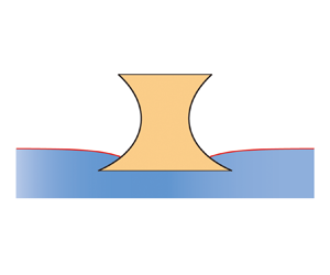
According to Archimedes’ principle, to press a floating solid object of macroscale into deeper water very slowly, the pressing force tends to get larger and larger due to an increasing volume of the immersed solid. However, this may not be the case for the floating object of mesoscale or microscale under surface tension effects. At a uniform contact angle, an exotic floating object of two-dimensional (2-D) or axial symmetry is proposed here, which can be pressed into (or pulled up from) the infinite liquid bath steadily by a constant vertical force $f$, as shown in figure 1. During the movement, the exotic floating object stays in force balance. If we regard this constant external force $f$ as an extra part of the constant weight of the exotic floating object, then it can be claimed that the exotic floating object can permit infinitely many continuous vertical equilibrium positions.

Figure 1. Cross-section schematic of a symmetric solid object floating in an unbounded liquid bath. For the 2-D-symmetric case, the origin of the dimensionless Cartesian coordinates $(x, u)$ is located on the symmetry axis (while for the axisymmetric case, the dimensionless cylindrical coordinates $(r, u)$ are used instead). The height of the undisturbed liquid surface at infinity is set as $u=0$. The (side) shape of this solid object at a contact angle $\theta$ is expressed as $x(y)$ for the 2-D-symmetric case, or $r(y)$ for the axisymmetric case. At the contact point $A$, $\varphi$ denotes the angle between the normal of the solid surface and the horizontal line; ${\tilde {\psi }}$ denotes the inclination angle of the meniscus. Here, $\varphi$ and $\tilde {\psi }$ are both measured anticlockwise starting from the positive $x$ axis. Under a constant vertical force $f$, the solid object moves down from the initial equilibrium configuration (see orange region and solid red curves) to another (see dashed black and dashed red curves). Points $A$ and $A'$ correspond to the same point on the solid for the two configurations.

2.1. Two-dimensional and axisymmetric menisci

Considering the meniscus in equilibrium, its shape is governed by the known Young–Laplace equation. The lengths are scaled relative to the capillary length ${l_c} = \sqrt {\sigma /{\rho }g}$, where $\sigma$ denotes the surface tension coefficient, and $\rho$ denotes the density difference between liquid and gas (while the density of the gas is neglected).

For the 2-D case, if the meniscus extends infinitely to the right (see red curves of $x>0$ in figure 1), then its dimensionless shape $\tilde {u}(\tilde {x})$ can be obtained by a first integral of the 2-D Young–Laplace equation (Huh & Scriven 1969; Finn 1986; Bhatnagar & Finn 2016), which gives

(2.1a)\begin{gather} \tilde{u} ={-}2\sin \dfrac{{\tilde{\psi} }}{2}, \end{gather}

(2.1b)\begin{gather}\tilde{x} - {\tilde{x}_0} ={-}2\cos \frac{\tilde{\psi} }{2} + 2 \cos \frac{{{\tilde{\psi} _0}}}{2} - \ln \left(\frac{\tan \tilde{\psi}/4}{\tan \tilde{\psi} _0/4}\right), \end{gather}

where $\tilde {(\,\cdot\,)}$ indicates that the quantity is related to the meniscus, ${\tilde {(\,\cdot\,)}_0}$ indicates that the quantity is evaluated for the meniscus at the contact point, and $\tilde {\psi }$ denotes the inclination angle of the meniscus (which varies for different points on the meniscus). The boundary condition for the meniscus at infinity is satisfied automatically in (2.1).

For the axisymmetric case, the dimensionless cylindrical coordinates $(r, u)$ and the dimensionless axisymmetric menisci shape $\tilde {u}(\tilde {r})$ are used instead. Accordingly, the exotic floating object and the surrounding menisci in figure 1 are regarded as axisymmetric. The Young–Laplace equation for the axisymmetric meniscus of unbounded extent can be expressed in the parametric form (Huh & Scriven 1969)

(2.2a,b)\begin{equation} \frac{{{\rm{d}}\tilde{r}(\tilde{\psi})}}{{{\rm{d}}\tilde{\psi} }} = \frac{{\tilde{r} \cos \tilde{\psi} }}{{{\tilde{r}} {\tilde{u}} - \sin \tilde{\psi} }}, \quad \frac{{{\rm{d}}\tilde{u}(\tilde{\psi})}}{{{\rm{d}}\tilde{\psi} }} = \frac{{\tilde{r} \sin \tilde{\psi} }}{{\tilde{r} \tilde{u} - \sin \tilde{\psi} }}. \end{equation}

The associated boundary conditions at the contact point give

(2.3)\begin{equation} \tilde{\psi} = {\tilde{\psi} _0}, \quad \text{for} \ \tilde{r}={\tilde{r}_0}. \end{equation}

For the associated boundary condition at infinity ($\tilde {r} \to + \infty$), both the values of $\tilde {\psi }$ and $\tilde {u}$ tend to 0, which makes it impractical to implement a numerical scheme for (2.2a,b) since the singularity occurs at $\tilde {u}=\tilde {\psi }=0$. Therefore, an asymptotic prediction at very small values of $\tilde {u}$ and $\tilde {\psi }$ is used as the boundary condition far from the contact point, which is given by (Huh & Scriven 1969)

(2.4)\begin{equation} {\tilde{u}^ * } ={-} \tan {\tilde{\psi} ^ * }\,{{\rm K}_0}({\tilde{r}^*})/{{\rm K}_1}({\tilde{r}^*}), \quad \text{for} \ \tilde{r}=\tilde{r}^*, \end{equation}

where ${\rm K}_i$ denotes the modified Bessel function of the second kind of order $i$ ($i=0$ and 1 here). As $\tilde {\psi }^*$ tends to 0, $\tilde {u}^ *(\tilde {r}^ *)$ in (2.4) exhibits good convergence and accuracy as the asymptotic solution of the Young–Laplace equation in the axisymmetric case (Huh & Scriven 1969). In our calculations, $\tilde {\psi }^*$ of small value is set as $\tilde {\psi }^*=\pm 0.001^\circ$, where the sign is the same as $\tilde {\psi }_0$ in (2.3). The shooting method is used to solve the two-point boundary value problem (2.2)–(2.4). By guessing a value of $\tilde {r}^*>0$, we can integrate (2.2) numerically from the initial point $\tilde {\psi }=\tilde {\psi }^*$ to the end point $\tilde {\psi }= \tilde {\psi }_0$ with the Runge–Kutta method. At $\tilde {\psi }=\tilde {\psi }_0$, $\tilde {r}$ may not be equal to $\tilde {r}_0$, so the secant method is applied to adjust $\tilde {r}^*$ to satisfy (2.3). With a proper $\tilde {r}^*$, the axisymmetric meniscus shape $\tilde {u}(\tilde {r})$ satisfying (2.2)–(2.4) can be determined.

2.2. Force analysis for symmetric floating objects

Although dimensionless lengths have been adopted in § 2.1, we use the dimensional forms for all physical quantities to aid in the comprehension of the force derivation temporarily. But at the end of this derivation, the dimensionless scaling will be adopted again. For a floating object of arbitrary shape in two dimensions, Zhang et al. (2018) proposed a convenient model to calculate its vertical resultant force (including the weight force and the total force exerted by the liquid), which is obviously applicable for 2-D-symmetric floating objects. Our investigation suggests that this model can also be extended to the axisymmetric floating objects.

The forces acting on the 2-D-symmetric or axisymmetric floating object are the surface tension force $\boldsymbol {F}_\sigma$, the hydrostatic pressure force $\boldsymbol {F}_p$ and the weight force $\boldsymbol {F}_g$, as shown in figure 2. The total force exerted by the liquid is the sum of $\boldsymbol {F}_\sigma$ and $\boldsymbol {F}_p$. The vertical component of the surface tension force can be expressed as

(2.5)\begin{equation} {F_{\sigma ,v}} = \left\{ \begin{array}{@{}ll} 2\sigma \sin \psi, & \text{for the 2-D-symmetric case},\\ 2{\rm \pi} R_0 \sigma \sin \psi, & \text{for the axisymmetric case}, \end{array} \right. \end{equation}

where $\psi$ denotes the inclination angle of the meniscus for the contact point on the solid surface. For the floating object with an undetermined vertical position, $\psi$ varies as the contact point moves on the solid surface. Obviously, there is $\psi =\tilde {\psi }_0$ for a prescribed position of the contact point. The vertical component of the hydrostatic pressure force is calculated by integrating the hydrostatic pressure $p$ (where $p=-\rho g U$) over the wetted solid surface (see thick black curve $\varSigma$ in figure 2), which gives

(2.6)\begin{equation} {F_{p ,v}} = \left\{ \begin{array}{@{}ll} \displaystyle -\int_\varSigma {\rho g U\sin \alpha \, {\rm{d}}s}, & \text{for the 2-D-symmetric case},\\ \displaystyle-\int_\varSigma {2{\rm \pi} R\rho g U\sin \alpha \, {\rm{d}}s}, & \text{for the axisymmetric case}, \end{array} \right. \end{equation}

where $s$ denotes the arc length coordinate, and $\alpha$ denotes the direction angle of the local hydrostatic pressure (see figure 2). The local hydrostatic pressure is always normal to the solid surface, which implies the relationship $\sin \alpha \, {\rm {d}}s = {\rm {d}} X$ (or $\sin \alpha \, {\rm {d}}s = {\rm {d}} R$).

Figure 2. Force diagram for a symmetric solid object floating in an infinite liquid bath. For the 2-D-symmetric case, the dimensional Cartesian coordinate system $({X},{U})$ is utilized, while for the axisymmetric case, the dimensional cylindrical coordinate system $( R, U)$ is utilized. The contact point on the right locates at $(X_0, U_0)$ or $(R_0, U_0)$. The anticlockwise thick black curve (or generatrix) $\varSigma$ and blue curve (or generatrix) $\varSigma {'}$ correspond to the wetted solid surface and the waterline, respectively. The submerged solid part (orange region) is enclosed by $\varSigma$ and $\varSigma {'}$. The surface tension $\sigma$, the actual hydrostatic pressure $p$, and the fictitious hydrostatic pressure $p'$ are denoted by green, orange and dashed blue arrows, respectively. The direction angle $\alpha$ for the local hydrostatic pressure is measured anticlockwise from the positive $X$ axis.

Following Zhang et al. (2018), we imagine that there exists fictitious hydrostatic pressure $p'=-\rho g U_0$ acting on the waterline (see blue curve $\varSigma '$ and dashed blue arrows in figure 2). Applying Green's theorem for the anticlockwise closed curve merged by $\varSigma$ and $\varSigma '$, we have

(2.7)\begin{equation} \left. \begin{array}{ll@{}} \displaystyle-\oint_{\varSigma + \varSigma '} {\rho g U\sin \alpha \, {\rm{d}}s = \rho g{S_b}}, & \text{for the 2-D-symmetric case},\\ \displaystyle-\oint_{\varSigma + \varSigma '} {2{\rm \pi} R\rho g U\sin \alpha \, {\rm{d}}s = \rho g{V_b}}, & \text{for the axisymmetric case}, \end{array} \right\} \end{equation}

where $S_b$ ($V_b$) denotes the area (volume) of the solid part immersed in liquid (see orange region in figure 2). For the waterline $\varSigma '$, we have $U=U_0$ and $\alpha =-{\rm \pi} /2$. Thus the fictitious pressure force acting on $\varSigma '$ can be reduced to the form

(2.8)\begin{equation} \left. \begin{array}{ll@{}} \displaystyle-\int_{ \varSigma '} {\rho g U\sin \alpha \, {\rm{d}}s = 2\rho g X_0 U_0 }, & \text{for the 2-D-symmetric case},\\ \displaystyle-\int_{ \varSigma '} {2{\rm \pi} R\rho g U\sin \alpha \, {\rm{d}}s = \rho g {\rm \pi}R_0^2 U_0 }, & \text{for the axisymmetric case}, \end{array} \right\} \end{equation}

where the integration on ${ \varSigma '}$ is performed from right to left. Comparing (2.6)–(2.8), the vertical component of the hydrostatic pressure force can be expressed in the simple form

(2.9)\begin{equation} {F_{p ,v}} = \left\{ \begin{array}{@{}ll} \rho g (S_b-2 X_0 U_0), & \text{for the 2-D-symmetric case},\\ \rho g (V_b-{\rm \pi} R_0^2 U_0), & \text{for the axisymmetric case}. \end{array} \right. \end{equation}

Adding the three vertical force components $F_{\sigma,v}$, $F_{p ,v}$ and $F_{g}$ (norm of the weight force $\boldsymbol {F}_g$), we can obtain the dimensional vertical resultant force

(2.10)\begin{equation} {F_v} = \left\{\begin{array}{@{}ll} 2\sigma \sin \psi+ \rho g (S_b-2 X_0 U_0)-F_g, & \text{for the 2-D-symmetric case},\\ 2{\rm \pi} R_0 \sigma \sin \psi+\rho g (V_b-{\rm \pi} R_0^2 U_0)-F_g, & \text{for the axisymmetric case}. \end{array} \right. \end{equation}

The following dimensionless sizes (including the area or volume) and dimensionless force components are used in this paper:

(2.11)\begin{equation} \left. \begin{array}{ll@{}} \displaystyle \left\{ {{\,f_{v}},{f_g}} \right\} = \dfrac{{\left\{ {{F_v},{F_g}} \right\}}}{\sigma },\quad\left\{ {{x},{u},{s_b}} \right\} = \dfrac{{\left\{ {{ X_0},{U_0},{S_b/l_c}} \right\}}}{{{l_c}}}, & \text{for the 2-D-symmetric case},\\ \displaystyle \left\{ {{\,f_{v}},{f_g}} \right\} = \dfrac{{\left\{ {{F_v},{F_g}} \right\}}}{{\sigma {l_c}}},\quad\left\{ {{r},{u},{v_b}} \right\} = \dfrac{{\left\{ {{R_0},{U_0},{V_b/l_c^2}} \right\}}}{{{l_c}}}, & \text{for the axisymmetric case}. \end{array} \right\} \end{equation}

Substituting (2.11) into (2.10), the dimensionless form of the vertical resultant force gives

(2.12a,b)\begin{equation} {f_v} = \left\{ \begin{array}{@{}ll} 2 \sin \psi+ s_b-2 x u-f_g, & \text{for the 2-D-symmetric case},\\ 2{\rm \pi} r \sin \psi + v_b-{\rm \pi} {r}^2 u - f_g, & \text{for the axisymmetric case}. \end{array} \right. \end{equation}

For a prescribed contact point, the dimensionless height $u$ can be obtained from (2.1a) for the 2-D-symmetric case, or from the ordinary differential equation (ODE) system (2.2)–(2.4) for the axisymmetric case. Notably, (2.12) is applicable under the precondition that the menisci around the floating object are stable; otherwise, the floating configuration cannot exist in practice.

For the exotic floating object of constant weight $f_g$ in both the 2-D-symmetric and axisymmetric cases, its ‘exotic’ property indicates that the vertical resultant force $f_{v}$ remains constant no matter where the exotic floating object locates vertically, which gives

(2.13)\begin{equation} f_v \equiv {\rm const.} \end{equation}

for the exotic floating object; $f_v$ of non-zero constant can be counterbalanced by the constant external force $f$ (see in figure 1), where $f=-f_{v}$. With (2.12) and (2.13), the relation between the ‘exotic’ property and the geometrical shape for the exotic floating object will be constructed. Only the vertical equilibrium is considered because the horizontal equilibrium and the rotational equilibrium are satisfied automatically from the symmetry of the exotic floating object.

2.3. Curvatures of the exotic floating objects

To determine directly the shape for the exotic floating object may be challenging, while it is relatively easy to derive the curvature of the exotic floating object as a transitional approach, from which the shape can also be obtained.

2.3.1. Two-dimensional-symmetric case

To determine the shape of a solid object moving vertically, it is advantageous to utilize the coordinate system $(x,y)$ that is fixed to the object. This system $(x,y)$ is linked to the coordinate system $(x, u)$ fixed to the liquid through the floating height $h$ (defined as the $u$ coordinate of $y=0$ on the solid object; see points $A$ and $A'$ in figure 1):

(2.14)\begin{equation} y=u-h. \end{equation}

Due to the symmetry, only the right half configuration of $x \ge 0$ is considered. Introducing the arc length $s$, the solid shape $x(y)$ can be expressed in the parametric form

(2.15a–c)\begin{equation} \frac{{{\rm{d}}\,x(s)}}{{{\rm{d}}s}} ={-} \sin \varphi ,\quad \frac{{{\rm{d}}y(s)}}{{{\rm{d}}s}} = \cos \varphi\quad {\rm{and}}\quad\frac{{{\rm{d}}\varphi(s) }}{{{\rm{d}}s}} = K, \end{equation}

where $K$ in (2.15c) denotes the dimensionless curvature of the solid surface ($K > 0$ if the solid surface is convex to the liquid). Once the curvature $K$ is derived, the whole solid shape curve can be obtained accordingly. In (2.15c), $\varphi$ denotes the angle between the normal of $x(y)$ and the horizontal line (see figure 1). According to Young's relation, the normal angle $\varphi$ for the solid surface is related to the inclination angle $\psi$ for the liquid surface as

(2.16)\begin{equation} \psi = \theta + \varphi - {{\rm \pi} }/{2}, \quad \text{at the contact point}, \end{equation}

where $\theta$ denotes the constant contact angle, and $\psi$ and $\varphi$ depend on the position of the contact point on the solid surface (i.e. they are both functions of $s$).

For the exotic floating object, the contact point changes with the floating height $h$. In the two coordinate systems (fixed to the solid and the liquid), both the coordinates $(x,y)$ and $(x,u)$ for the contact point are variable. For the 2-D-symmetric case, the differential of the (constant) vertical resultant $f_v$ in (2.12a) gives

(2.17)\begin{equation} {\rm{d}}{f_v} = {\rm{d}}{s_b} - 2(x\,{\rm{d}}u + u\,{\rm{d}}\,x) + 2\sin (\varphi + \theta )\,{\rm{d}}\varphi \equiv 0, \end{equation}

where ${\rm {d}}{s_b}$ denotes the differential of the solid area submerged in the liquid, given in simple form by ${\rm {d}}{s_b}=2x\,{\rm {d}}y$. The first two terms in the middle represent the variation of the hydrostatic pressure force, while the last term in the middle represents the variation of the surface tension force. Essentially, the ‘exotic’ property is due to the relation that these two variations keep counteracting each other.

In order to derive the curvature $K$ in (2.15c), we try to transform ${\rm {d}}f_v$ in terms of ${{\rm {d}}s}$. From (2.1a) and (2.16), ${\rm {d}}u$ at the contact point can be expressed as

(2.18)\begin{equation} {\rm{d}}u={-}{{\sin \frac{{{\rm \pi} + 2(\theta + \varphi )}}{4}}} \,{\rm{d}}\varphi. \end{equation}

Substituting (2.1a) and (2.18) into (2.17), ${\rm {d}}{f_v}$ can be expressed in terms of ${\rm {d}}\,x$, ${\rm {d}}y$ and ${\rm {d}}\varphi$. With (2.15a–c), ${\rm {d}}{f_v}$ is then expressed in terms of ${\rm {d}}s$ only:

(2.19)\begin{equation} {\rm{d}}f_v=2\left[x\cos \varphi + 2\cos \frac{{{\rm \pi} + 2(\theta + \varphi )}}{4} + { K }\sin (\theta + \varphi )+ { K } x\sin \frac{{{\rm \pi} + 2(\theta + \varphi )}}{4}\right]\,{\rm{d}}s. \end{equation}

By letting ${\rm {d}}f_v$ in (2.19) be equal to zero, the solid surface curvature of the exotic floating object for the 2-D-symmetric case can be obtained as

(2.20)\begin{equation} \bar{K}_{2\text{-}D}={-} \frac{{x\cos \varphi + 2\cos \dfrac{{{\rm \pi} + 2(\theta + \varphi )}}{4}\sin \varphi }}{{\sin (\theta + \varphi ) + x\sin \dfrac{{{\rm \pi} + 2(\theta + \varphi )}}{4}}}. \end{equation}

Substituting this curvature $\bar {K}_{2\text {-}D}$ into (2.15c), the shape $x(y)$ of the 2-D-symmetric exotic floating object can be obtained by solving (2.15a–c).

2.3.2. Axisymmetric case

For the axisymmetric exotic floating object, we adopt the cylindrical coordinate system $(r, y)$ fixed to the solid to determine its shape. Similar to the 2-D-symmetric case, the generatrix $r(y)$ (where $r\ge 0$) can be expressed in the parametric form of the arc length $s$:

(2.21a–c)\begin{equation} \frac{{{\rm{d}}r(s)}}{{{\rm{d}}s}} ={-} \sin \varphi ,\quad \frac{{{\rm{d}}y(s)}}{{{\rm{d}}s}} = \cos \varphi \quad {\rm{and}}\quad \frac{{{\rm{d}}\varphi (s)}}{{{\rm{d}}s}} = K, \end{equation}

where $K$ denotes the dimensionless generatrix curvature of the solid surface ($K>0$ if the generatrix is convex to the liquid).

Following Zhang et al. (2018), we have developed an approach to calculating the vertical resultant force for the axisymmetric floating object in (2.12b). Analogous to (2.17), we give the differential of the (constant) vertical resultant $f_v$ in (2.12b) for the axisymmetric exotic floating object as

(2.22)\begin{equation} {\rm{d}}f_v={\rm{d}}v_b - {\rm \pi}{r^2}\,{\rm{d}}u - 2{\rm \pi} [ru + \cos (\theta + \varphi )]\,{\rm{d}}r + 2{\rm \pi} r\sin (\theta +\varphi )\,{\rm{d}}\varphi \equiv 0, \end{equation}

where the differential of the submerged solid volume is ${\rm {d}}v_b={\rm \pi} r^2\, {\rm {d}}y$.

For the axisymmetric case, the height $u$ at the contact point depends on both the corresponding radius $r$ and inclination angle $\psi$, while it depends only on $\psi$ for the 2-D-symmetric case from (2.1a). At the contact point, the differential ${\rm {d}}u$ for the axisymmetric case can be expressed as

(2.23)\begin{equation} {\rm{d}}u(r,\psi) = \frac{{\partial u}}{{\partial r }}\,{\rm{d}}r + \frac{{\partial u}}{{\partial \psi}}\,{\rm{d}}\psi, \end{equation}

where $u$ is short for $u(r,\psi )$ on the right-hand side. At the contact point, the values of ${{\partial u}}/{{\partial r}}$ and ${{\partial u}}/{{\partial \psi }}$ can be obtained during the determination of the corresponding axisymmetric meniscus, which is seen in Appendix A.

From Young's relation (2.16), we have ${\rm {d}}\psi ={\rm {d}}\varphi$ for (2.23). Substituting (2.23) into (2.22), ${\rm {d}}{f_v}$ can be expressed in terms of ${\rm {d}}r$, ${\rm {d}}y$ and ${\rm {d}}\varphi$, while these three can all be expressed in terms of ${\rm {d}}s$ by (2.21a–c). Then ${\rm {d}}{f_v}$ for the axisymmetric case is given by

(2.24) \begin{align} {\rm{d}}{f_v} &= {\rm \pi} \left\{ \left[2\cos (\theta + \varphi ) + 2ru + {r^2}\,\frac{{\partial u}}{{\partial r}}\right]\sin \varphi \right.\nonumber\\ &\left.\quad + r\left[2{{K}}\sin (\theta + \varphi ) - r{{ K}}\,\frac{{\partial u}}{{\partial \psi }} + r\cos \varphi \right]\right\} \,{\rm{d}}s. \end{align}

For the exotic floating object, ${\rm {d}}{f_v}$ in (2.24) is equal to zero, from which we can obtain its generatrix curvature:

(2.25)\begin{equation} {{\bar{K}}_{axi}} = \frac{{{r^2}\cos \varphi + 2\sin \varphi\,[ru + \cos (\theta + \varphi )] + {r^2}\sin \varphi\,\dfrac{{\partial u}}{{\partial r}} }}{{ - 2r\sin (\theta + \varphi ) + {r^2}\,\dfrac{{\partial u}}{{\partial \psi }}}}. \end{equation}

In this paper, $(\,\cdot\,)_{axi}$ denotes the quantity for the axisymmetric case. Substituting this curvature $\bar {K}_{axi}$ into (2.21c) and solving (2.21a–c), the generatrix shape $r(y)$ of the axisymmetric exotic floating object can be determined.

3. Shape determination and existence of the exotic floating objects

3.1. Shapes of the exotic floating objects

With the curvatures given in (2.20) and (2.25), the shapes of the 2-D-symmetric and axisymmetric exotic floating objects are obtained in this subsection. Through the Runge–Kutta integration, the two ODE systems (2.15a–c) and (2.21a–c) are solved with the initial conditions

(3.1)\begin{equation} \left. \begin{array}{ll@{}} x = {x_i},\ y = {y_i}\ {\rm{and}}\ \varphi = {\varphi _i}, & \text{for the 2-D-symmetric case},\\ r = {r_i},\ y = {y_i}\ {\rm{and}}\ \varphi = {\varphi _i}, & \text{for the axisymmetric case}, \end{array} \right\} \end{equation}

respectively. Since $\bar {K}_{2\text {-}D}$ in (2.20) and $\bar {K}_{axi}$ in (2.25) are both independent of $y$, the initial value $y_i$ can be chosen arbitrarily, which will not influence the shape of the exotic floating object but just change its vertical position. Without loss of generality, we set $y_i = 0$ in our calculations. Examples of exotic shape curves with the contact angle $\theta ={\rm \pi} /3$ and the initial point $(x_i, y_i)$ or $(r_i, y_i)=(1, 0)$ are given in figure 3. Selecting an arbitrary part of $x\ge 0$ or $r \ge 0$ for an exotic shape curve as the solid surface, we can obtain the corresponding exotic floating object (see thick black curves and the corresponding inset in figure 3b). With the increase of $\varphi _i$ from $-{\rm \pi} /2$ to ${\rm \pi} /2$ (see figure 3a), three distinct types of exotic shape curves are observed for both the 2-D-symmetric case (see left-hand images in figures 3b–d) and the axisymmetric case (see right-hand images in figures 3b–d). When exploring various initial points and contact angles, we have not discovered any additional types beyond these three.

Figure 3. Types of shape curves for the exotic floating objects at the contact angle $\theta ={\rm \pi} /3$ and the initial point $(x_i, y_i)$ or $(r_i, y_i)=(1, 0)$. (a) Parameter intervals of $\varphi _i$ for types I, II and III. The left-hand (right-hand) image corresponds to the 2-D-symmetric (axisymmetric) case, similar to the other pairs of plots below. (b–d) Exotic shape curves (in black) for types I, II and III, respectively. Each red curve denotes a possible meniscus (for some floating height $h$), and the blue circles in (b,d) denote singular points with infinitely large curvatures. The insets in (b) show the exotic floating objects corresponding to the thick black curves.

No significant difference is found between the same type of exotic shape curves for the 2-D-symmetric case and the axisymmetric case. The exotic shape curves of type II (in figure 3c) stay concave to the liquid. In other words, $\bar {K}_{2\text {-}D}<0$ or $\bar {K}_{axi}<0$ for type II. However, for types I and III (in figures 3b,d), the exotic shape curves are partially convex and partially concave to the liquid, each with an inflection point (where $\bar {K}_{2\text {-}D}=0$ or $\bar {K}_{axi}=0$). The inflection points of the exotic shape curves in figures 3(b,d) are set on the $y$ axis deliberately, with the result that the exotic shape curves of type I (III) are convex (concave) to the liquid for $y<0$, and concave (convex) to the liquid for $y>0$. In addition, on the exotic shape curve of type I or type III, there exists a singular point (see blue circles in figures 3b,d) where the curvature $\bar {K}_{2\text {-}D}$ in (2.20) or $\bar {K}_{axi}$ in (2.25) tends towards positive infinity.

3.2. Stabilities of menisci around the exotic floating object

Despite the determination of the exotic floating object, the corresponding exotic flotation phenomenon may not exist in practice due to the instabilities of the menisci around it. Especially for the concave solid surface (see examples in figures 3b–d), the menisci around it are more likely to be unstable and reconfigure spontaneously (Tan et al. 2022). To examine the meniscus stabilities, the direct computation method (Myshkis et al. 1987; Slobozhanin & Perales 1993; Pesci et al. 2015) can be a viable option by solving the eigenvalue problem related to the second variation of the total energy functional, while the direct computation method has been developed further into a critical parameter comparison method (Zhang & Zhou 2020a,b), which enables us to determine the meniscus stabilities with only the physical parameters at the contact point. For convenience, the critical parameter comparison method is utilized in this subsection to determine the stabilities of menisci around the exotic floating object.

3.2.1. Two-dimensional-symmetric case

To find out whether a 2-D meniscus without volume constraint is stable or not, the potential energy functional of the whole capillary system can be derived. The second variation of the potential energy functional gives the unified eigenvalue problem in two dimensions (Myshkis et al. 1987; Bostwick & Steen 2015; Zhang & Zhou 2020a):

(3.2)\begin{equation} \left. \begin{array}{ll@{}} {-\phi _0''}+ (3\cos \psi -{{ 2)}}{\phi _0} = \lambda {\phi _0}, & \text{for the meniscus},\\ {\phi _0'} + {\chi}{\phi _0} = 0, & \text{at the contact point}, \end{array} \right\} \end{equation}

where $\phi _0$ denotes the allowable disturbance for the 2-D meniscus, $(\,\cdot\,)'$ denotes the derivative with respect to the arc length $s$ along the meniscus, $\lambda$ denotes the eigenvalue, and the boundary parameter $\chi$ of the solid surface at the contact point is expressed as (Zhang & Zhou 2020a)

(3.3)\begin{equation} {{{\chi }}} = \frac{{ -2\sin \dfrac{{ \psi }}{2} \cos \theta + K }}{{\sin \theta }}, \end{equation}

where $K$ denotes the signed curvature of the solid surface at the contact point. It should be noted that in this study, the right half configuration (of $x\ge 0$) is considered, and the curvature of the solid surface convex towards the liquid is defined as positive, possibly leading to a sign difference between (3.3) and the literature (e.g. Zhang & Zhou 2020a; Tan et al. 2022).

The eigenvalues of the Sturm–Liouville problem (3.2) are real and can be sorted as $\lambda _1<\lambda _2<\lambda _3<\cdots <\lambda _n<\cdots <+\infty$. The lowest eigenvalue $\lambda _1$ in (3.2) dictates the stabilities of the meniscus. Specifically, the meniscus is stable (unstable) if $\lambda _1>0$ ($\lambda _1<0$), and the stable meniscus indicates a local minimum of the potential energy functional. It is feasible but laborious to solve (3.2) directly for the value of $\lambda _1$, so an alternative approach is employed here. According to the modal monotonicity (Myshkis et al. 1987; Bostwick & Steen 2015), the function $\lambda _1(\chi )$ increases monotonically with $\chi$. Consequently, there can exist a critical boundary parameter $\chi ^*$ satisfying $\lambda _1(\chi ^*)=0$, and the stable condition $\lambda _1>0$ for the meniscus is equivalent to

(3.4)\begin{equation} {{{\chi }}} - {{\chi }}^ * > 0. \end{equation}

The total potential energies for all possible equilibrium menisci around the exotic cylinder are exactly the same (Wente 2011; Zhang & Zhou 2020a). This remarkable property indicates that all the possible menisci around the exotic cylinder are in critical stable states of $\lambda _1=0$ and $\chi =\chi ^*$, which has been shown in Zhang & Zhou (2020a). It should be emphasized that the proposed exotic floating object is distinct from the exotic cylinder (which is typically considered as stationary, not floating). The related discussion about the exotic cylinder is available in Appendix B. For a certain meniscus meeting a certain solid surface (with $\psi$ and $\theta$ known in (3.3)), substituting the (critical) curvature $K_{2\text {-}D}^*$ of the 2-D exotic cylinder in (B3) into (3.3), we can obtain the critical boundary parameter $\chi ^*$ for the 2-D case as

(3.5)\begin{equation} {{\chi }}^ * ={-} \frac{{\cos \psi }}{{\cos \dfrac{\psi }{2}}}. \end{equation}

Using the critical parameter comparison method (3.3)–(3.5), the stability of a 2-D meniscus meeting an arbitrary solid surface can be determined. This method is used to predict the stabilities of menisci around the exotic floating object. As the floating height $h$ changes, every point on the solid surface of the exotic floating object may serve as the contact point, and every contact point corresponds to a meniscus in equilibrium. At a given contact point, the curvature of the solid surface can be obtained from (2.20), and the meniscus inclination angle can be obtained from (2.16), enabling the calculation of both the boundary parameter $\chi$ in (3.3) and the critical boundary parameter $\chi ^*$ in (3.5). The stabilities of all the possible menisci around the 2-D-symmetric exotic floating object are then assessed using the criterion (3.4).

For the shape curves of the 2-D-symmetric exotic floating objects (in figure 3), the values of ${{{\chi }}} - {{\chi }}^ *$ at different contact points are shown in figure 4. All the possible menisci around these 2-D-symmetric exotic floating objects are stable because ${{{\chi }}} - {{\chi }}^ *>0$. At a large value of $x$, ${{{\chi }}} - {{\chi }}^ *$ for the exotic floating object of type I and type III is close to that of type II. This is because the exotic curve shapes of type I and type III (in figures 3b,d) become increasingly similar to those of type II (in figure 3c) as $x$ increases. As $x$ decreases for type I and type III, the contact point gets closer to the singular point (see blue circles in figures 3b,d), and the meniscus stability is enhanced due to the increase of the (convex) solid surface curvature. For a singular contact point of positive infinite curvature, the corresponding meniscus is actually pinned at a sharp edge (Zhang & Zhou 2020b), whose stability is the most stable (with ${{{\chi }}} - {{\chi }}^ * \to +\infty$).

Figure 4. The meniscus stabilities for different contact points on the 2-D-symmetric exotic floating objects. The boundary parameters are obtained from the shape curves of the 2-D-symmetric exotic floating objects (see black curves in left-hand images of figures 3b–d). All the corresponding menisci are stable because ${{\chi } - {\chi}^ *>}0$.

3.2.2. Axisymmetric case

Previous research (e.g. Myshkis et al. 1987; Slobozhanin & Alexander 2003) has shown that axisymmetric disturbances pose a greater threat to the stability of an axisymmetric meniscus in the absence of volume constraint, compared to non-axisymmetric disturbances. Consequently, considering only the axisymmetric disturbance is sufficient for stability analysis on the axisymmetric menisci. Under the axisymmetric disturbance, the eigenvalue problem for the axisymmetric meniscus is given by (Myshkis et al. 1987; Bostwick & Steen 2015; Zhang & Zhou 2020a)

(3.6)\begin{equation} \left. \begin{array}{ll@{}} \displaystyle - {\phi _0''} - \dfrac{{r'}}{r}\,{\phi _0'} + \Bigg[\cos \psi - (\psi ')^2 - \dfrac{{{\sin^{{2}}}\psi }}{{{r^{{2}}}}}\Bigg]\phi _0 = \lambda {\phi _0}, & \mbox{for the meniscus},\\ {\phi _0'} + {\chi}{\phi _0} = 0, & \text{at the contact point}, \end{array} \right\} \end{equation}

where $(\,\cdot\,)'$ denotes the derivative with respect to the arc length $s$ along the meniscus generatrix. The boundary parameter $\chi$ of the solid surface generatrix at the contact point is expressed as (Myshkis et al. 1987; Bostwick & Steen 2015; Zhang & Zhou 2020a)

(3.7)\begin{equation} \chi = \frac{{\left(u - \dfrac{{\sin \psi }}{r}\right)\cos \theta + K }}{{\sin \theta }}, \end{equation}

where the height $u$ at the contact point is determined by the ODE system (2.2)–(2.4), and $K$ denotes the curvature of the solid surface generatrix at the contact point.

Due to the modal monotonicity (Myshkis et al. 1987; Bostwick & Steen 2015), the stable condition that the lowest eigenvalue satisfies $\lambda _1(\chi )>0$ can be transformed into the comparison of the boundary parameter and the critical one:

(3.8)\begin{equation} {{{\chi }}} - {{\chi }}^ * > 0. \end{equation}

Similar to the 2-D case, all the possible menisci around the axisymmetric exotic cylinder are also in critical stable states of $\lambda _1=0$ and $\chi =\chi ^*$ (Zhang & Zhou 2020a). For the axisymmetric meniscus, the critical boundary parameter $\chi ^*$ is obtained by substituting the (critical) generatrix curvature $K_{axi}^*$ of the axisymmetric exotic cylinder in (B6) together with the partial derivative relation (A2) into (3.7), which gives

(3.9)\begin{equation} {\chi ^*} = \frac{{\cos \psi + \sin \psi\,\dfrac{{\partial u}}{{\partial r}}}}{{\dfrac{{\partial u}}{{\partial \psi }}}}, \end{equation}

where the determination of ${{\partial u}}/{{\partial r}}$ and ${{\partial u}}/{{\partial \psi }}$ at the contact point is discussed in Appendix A. Using the critical parameter comparison method (3.7)–(3.9), the stability of an axisymmetric meniscus meeting an arbitrary solid surface of axial symmetry can be determined.

For a variable floating height $h$, the menisci around the axisymmetric exotic floating object may meet any (contact) point on the generatrix of the axisymmetric exotic floating object. The meniscus stabilities are assessed using the criterion (3.8). For the shape curves of the axisymmetric exotic floating objects in figure 3, the associated values of ${{{\chi }}} - {{\chi }}^ *$ are shown in figure 5. The curves of ${{{\chi }}} - {{\chi }}^ *$ for the axisymmetric case are similar to the 2-D-symmetric case (in figure 4), and all the possible menisci around these axisymmetric exotic floating objects are stable. For the exotic curves with the initial condition $x_i>0$ or $r_i>0$ and $-{\rm \pi} /2\le \varphi _i \le {\rm \pi}/2$, we have not found any unstable equilibrium meniscus around the exotic floating object at a contact angle $\theta$ between 0 and ${\rm \pi}$. In conclusion, the exotic flotation phenomenon can exist in practice.

Figure 5. The meniscus stabilities for different contact points on the axisymmetric exotic floating objects. The boundary parameters are obtained from the shape curves for the axisymmetric exotic floating objects (see black curves in right-hand images of figures 3b–d). All the corresponding menisci are stable because ${{{\chi }}} - {{\chi }}^ *>0$.

4. New method for floating stability analysis of general symmetric floating objects

For the interfacial flotation, not only the menisci but also the floating object can be unstable. Accordingly, the stabilities can be classified into the meniscus stabilities for liquid surfaces and the floating stabilities for solid objects. The critical parameter comparison method (see (3.3)–(3.5) and (3.7)–(3.9)) to assess the meniscus stabilities has been inspired by the exotic cylinder (Zhang & Zhou 2020a,b). Likewise, from the proposed exotic floating object, a new method can also be developed to analyse the (vertical) stabilities of general symmetric floating objects.

4.1. Two-dimensional-symmetric case

For a solid floating object (regardless of dimensions, symmetry and shape) in an equilibrium state (i.e. $f_v=0$), its vertical stability can be predicted by the vertical resultant force profile (Bhatnagar & Finn 2006; Chen & Siegel 2018; Zhang et al. 2018). The floating object is vertically stable if

(4.1)\begin{equation} \frac{{\rm{d}}\,{f_v}}{{\rm{d}}h} < 0, \end{equation}

i.e. the movement direction of the solid (sign of ${\textrm {d}h}$) is opposite to the direction of the corresponding restoring force (sign of ${\textrm {d}{f_v}}$). Generally, we will try to obtain the function $f_v(h)$ to use (4.1) directly. Nevertheless, the determination of $f_v(h)$ may be arduous, as it is heavily dependent on the whole solid shape.

From (2.14), the floating height $h$ is related by the $u$ coordinate and the $y$ coordinate of the contact point. The differential of (2.14) gives

(4.2)\begin{equation} {\rm{d}}h={\rm{d}}u-{\rm{d}}y. \end{equation}

Substituting (2.18) and (2.15b,c) into (4.2) in turn, $\textrm {d}h$ for the 2-D-symmetric case can be expressed in terms of $\textrm {d}s$:

(4.3)\begin{equation} {\rm{d}}h ={-} \left[\cos\varphi + K \sin\frac{{\rm \pi} + 2(\theta + \varphi )}{4}\right]\,{\rm d}s. \end{equation}

For a 2-D-symmetric floating object, only the right half configuration of $x\ge 0$ is taken into account. Substituting (2.19) and (4.3) into (4.1) gives

(4.4)\begin{equation} \frac{{\rm{d}}{f_v}}{{\rm{d}}h} = \frac{x\cos \varphi + 2\cos \dfrac{{{\rm \pi} + 2(\theta + \varphi )}}{4}\sin \varphi + K \left[\sin (\theta + \varphi ) + x\sin \dfrac{{{\rm \pi} + 2(\theta + \varphi )}}{4}\right]}{ - \dfrac{1}{2}\left[\cos\varphi + K \sin\dfrac{{\rm \pi} + 2(\theta + \varphi )}{4}\right]}. \end{equation}

From (4.4), besides the the contact angle $\theta$, the floating stability is actually related to the geometrical parameters (i.e. $x$, $\varphi$ and $K$) at the contact point only, rather than the whole solid surface. Likewise, the meniscus stability is related to the parameters only at the contact point (see (3.3)–(3.5) or (3.7)–(3.9)), rather than the whole meniscus profile.

Comparing (4.4) and (2.20), the numerator on the right-hand side of (4.4) can be expressed in terms of $\bar {K}_{2\textrm {-}D}$. So the original stability criterion (4.1) can be expressed in terms of $\bar {K}_{2\textrm {-}D}$, giving the new stability criterion as

(4.5a,b) \begin{gather} \left. \begin{gathered} \dfrac{{{\rm{d}}{f_v}}}{{{\rm{d}}h}} = (K - {{\bar{K}}_{2\text{-}D}})m < 0, \\ m ={-} \dfrac{{2\left[\sin (\theta + \varphi ) + x\sin \dfrac{{{\rm \pi} + 2(\theta + \varphi )}}{4}\right]}}{{\cos \varphi + K\sin \dfrac{{{\rm \pi} + 2(\theta + \varphi )}}{4}}}. \end{gathered} \right\} \end{gather}

From (4.5), $\textrm {d}f_v/\textrm {d}h$ is equal to zero if the local curvature is $K=\bar {K}_{2\textrm {-}D}$. Similar to the exotic cylinder (whose curvature $K^*_{2\textrm {-}D}$ is critical for the 2-D meniscus stability), the curvature $\bar {K}_{2\textrm {-}D}$ of the exotic flotation is critical for the stabilities of 2-D-symmetric floating objects.

For a 2-D-symmetric floating object whose solid surface $x(y)$ is smooth and convex everywhere, such as horizontally placed uniform cylinders and ellipses, we can deduce ${{\textrm {d}y}}/{{\textrm {d}\,x}}{|_{x = 0}} = 0$ from the symmetry and $K>0$ from the convexity. This implies that there are two points of $x=0$ on the solid surface with $\varphi ={\rm \pi} /2$ and $-{\rm \pi} /2$, and $\varphi$ is monotonic along the right half solid surface (see (2.15c)). Thus, on the smooth and convex solid surface, we have $-{\rm \pi} /2 \le \varphi \le {\rm \pi}/2$ and $K>0$ for the right half side of $x\ge 0$. An observation can be made that if $-{\rm \pi} /2 \le \varphi \le {\rm \pi}/2$, $K>0$, $x\ge 0$ and $0 < \theta +\varphi < {\rm \pi}$, then every term of the numerator and the denominator in (4.5b) is at least non-negative. Noticing the negative sign on the right-hand side of (4.5b), it is clear that $m<0$ in (4.5) for this case, which can specially give a simpler form for (4.5a). The condition $0 < \varphi +\theta < {\rm \pi}$ is equivalent to $| \psi | < {\rm \pi}/2$ from Young's relation (2.16), and the condition $x\ge 0$ is the basic premise for (4.5). Therefore, with a smooth and convex solid surface, the 2-D-symmetric floating object is vertically stable when

(4.6)\begin{equation} K - {{\bar{K}}_{2\text{-}D}} > 0, \quad \text{for} \ | \psi | < {\rm \pi}/2 \end{equation}

at the contact point. The criterion (4.6) is a special case of $m<0$ for (4.5).

The stabilities of a uniform cylinder floating horizontally in an unbounded bath are studied using the criterion (4.5), as shown in figure 6. With $0<\varphi <{\rm \pi} /2$ for the contact point, it is easy to verify that all the possible menisci around the uniform cylinder of $\theta ={\rm \pi} /2$ are stable from (3.3)–(3.5), so the precondition for the flotation is satisfied. For a certain floating configuration (e.g. in figure 6b), it is assumed that the corresponding weight force $f_g$ can achieve the vertical balance of forces (i.e. $f_{v}=0$). Excellent agreement is found in figure 6(a) between our theoretical prediction and the numerical result in Zhang et al. (2018), which has been non-dimensionalized in the scaling of this paper. From (2.16), the meniscus inclination angle at the contact point satisfies $|\psi |<{\rm \pi} /2$ for this neutral wetted uniform cylinder, so the floating stability can also be predicted by the special criterion (4.6). This criterion is used by comparing the local curvature $K$ of the solid surface and the critical curvature $\bar {K}_{2\textrm {-}D}$ of the corresponding exotic floating object. As is shown in figure 6(b), at the contact point the stable (unstable) floating configuration satisfies $K>\bar {K}_{2\textrm {-}D}$ ($K<\bar {K}_{2\textrm {-}D}$), while the critical stable floating configuration satisfies $K=\bar {K}_{2\textrm {-}D}$, which verifies the special criterion (4.6).

Figure 6. (a) Stability prediction for the horizontally floating uniform cylinder. The positive (negative) value of $\textrm {d}f_v/\textrm {d}h$ indicates unstable (stable) flotation. (b) The floating configurations for points $P_1$, $P_2$ and $P_3$ in (a). The red curves denote the menisci around the cylinder, and the blue dashed curves denote shape curves of the exotic floating objects that are generated from the contact points. The parameters for the uniform cylinder are the constant curvature (reciprocal of radius) $K=1.806$ and the contact angle $\theta ={\rm \pi} /2$.

4.2. Axisymmetric case

For the axisymmetric case, (4.1) and (4.2) are still applicable. Substituting (2.23) and (2.21a–c) into (4.2), together with $\textrm {d}\psi =\textrm {d}\varphi$ from (2.16), $\textrm {d}h$ can be expressed in terms of $\textrm {d}s$ as

(4.7)\begin{equation} {\rm{d}}h = \left( - \cos \varphi - \frac{{\partial u}}{{\partial r}}\sin \varphi + \frac{{\partial u}}{{\partial \psi }}\,K\right)\,{\rm{d}}s. \end{equation}

For an axisymmetric floating object, substituting (2.24) and (4.7) into (4.1), ${{\textrm {d}{f_v}}}/{{\textrm {d}h}}$ in the stability criterion (4.1) becomes

(4.8) \begin{equation} \frac{{{\rm{d}}{f_v}}}{{{\rm{d}}h}} ={-} \frac{{{\rm \pi} \left\{ {r^2}\cos \varphi + \left[2ru + {r^2}\,\dfrac{{\partial u}}{{\partial r}} + 2\cos (\theta + \varphi )\right]\sin \varphi + rK\left[ - r\,\dfrac{{\partial u}}{{\partial \psi }} + 2\sin (\theta + \varphi )\right]\right\} }}{{\cos \varphi + \sin \varphi\,\dfrac{{\partial u}}{{\partial r}} - K\,\dfrac{{\partial u}}{{\partial \psi }}}}. \end{equation}

Comparing (4.8) and (2.25), the numerator on the right-hand side of (4.8) can be expressed in terms of $\bar {K}_{axi}$. Therefore, the new stability criterion is given by

(4.9a,b) \begin{gather} \left. \begin{gathered} \dfrac{{{\rm{d}}{f_v}}}{{{\rm{d}}h}} = (K - {{\bar{K}}_{axi}})m < 0,\\ m = \dfrac{{{\rm \pi} r\left[r\,\dfrac{{\partial u}}{{\partial \psi }} - 2\sin (\theta + \varphi )\right]}}{{\cos \varphi + \sin \varphi\,\dfrac{{\partial u}}{{\partial r}} - K\,\dfrac{{\partial u}}{{\partial \psi }}}}. \end{gathered} \right\} \end{gather}

Also, the curvature $\bar {K}_{axi}$ of the exotic flotation is critical for the stability of axisymmetric floating objects.

Using the new criterion (4.9) in the axisymmetric case, we can predict the floating stability conveniently, without calculating the force profile, which may be troublesome for some complicated solid shape. The floating stabilities for an axisymmetric object of a selected generatrix shape $r(y)$ are shown in figure 7. This object is pressed into the liquid very slowly (to keep the force balance) with a vertical external force $f$. We can regard the external force as an extra part of the weight. Without the ‘exotic’ property of the exotic flotation, the external force $f$ is variable rather than constant.

Figure 7. (a) Floating object with the contact angle $\theta ={\rm \pi} /4$ and the generatrix shape $r(y) = 0.5 + 0.2\cos ({\rm \pi} + 2{\rm \pi} y)$. The red curves denote possible menisci (for different floating heights $h$), and the contact point on the thick black curve satisfies both conditions $\chi -\chi ^*>0$ and $\textrm {d}f_v/\textrm {d}h <0$, i.e. both the corresponding meniscus and flotation are stable. (b) Stabilities for the menisci with the contact point on $r(y)$. The grey region of $\chi -\chi ^*<0$ denotes unstable menisci. (c) Stabilities for the floating object with the contact point on $r(y)$. The grey region of $\textrm {d}f_v/\textrm {d}h >0$ denotes unstable flotation.

As the floating height $h$ changes, we assume that the equilibrium meniscus may meet any possible contact point at the solid surface generatrix $r(y)$ (see the menisci denoted by red curves in figure 7a). At a given contact point, both the local curvature $K$ and the normal angle $\varphi$ can be obtained from (2.21) with $\textrm {d}s=[(\textrm {d}r)^2+(\textrm {d}y)^2]^{1/2}$. For the contact point, to ensure that the corresponding floating configuration can be sustained, the meniscus stability is examined in figure 7(b) using the critical parameter comparison method, i.e. with (3.7)–(3.9). And then the floating stability is assessed in figure 7(c) using the proposed method, i.e. with the criterion (4.9). If the contact point is located on the generatrix where $\chi -\chi ^*>0$ and $\textrm {d}f_v/\textrm {d}h<0$ (see thick black curves in figure 7a), then the corresponding meniscus and the floating object are both stable, indicating that the flotation can exist in practice and is resilient.

An interesting observation is made in figure 7, that if the contact point satisfies the critical condition $\chi -\chi ^*=0$ for the meniscus stabilities, then $\textrm {d}f_v/\textrm {d}h \to \infty$ is also satisfied (see blue dashed lines in figures 7b,c). Comparing (4.9b) and (B6), if the local curvature is $K=K_{axi}^*$ in (4.9), then it is easy to prove that $m$ and $\textrm {d}f_v/\textrm {d}h$ in (4.9) will tend to infinity using Young's relation (2.16). Apparently, $m$ and $\textrm {d}f_v/\textrm {d}h$ in (4.5) also tend to infinity if $K=K_{2\textrm {-}D}^*$. Actually, for the exotic cylinder (of curvature $K_{2\textrm {-}D}^*$ or $K_{axi}^*$) permitting infinitely many menisci in equilibrium around it, neglecting the pinning of the contact line, any height disturbance $\Delta h$ will result in no equilibrium meniscus being permitted around it (as discussed in Appendix B; see figures 8b,c). In the system of statics, no equilibrium solution for the meniscus leads to the singularity when $K=K_{2\textrm {-}D}^*$ for the 2-D-symmetric case, or $K=K_{axi}^*$ for the axisymmetric case.

Figure 8. (a) Axisymmetric exotic cylinder at the contact angle $\theta ={\rm \pi} /3$ and the initial point $(r, u)=(1, 0)$, fixed at the initial height $h=0$. The red curves denote possible menisci. (b) The exotic cylinder floating at the initial height. The blue curve denotes the meniscus that can achieve the force balance for the exotic cylinder. (c) The exotic cylinder at the non-initial height. No meniscus in equilibrium is permitted around the exotic cylinder. The blue dashed and red dashed curves in (c) are the same as the corresponding curves in (b) except for the vertical locations.

In conclusion, the curvature of the proposed exotic floating object is critical for the floating stability (i.e. $\textrm {d}f_v/\textrm {d}h =0$), while the curvature of the exotic cylinder is critical for the meniscus stabilities (i.e. $\chi -\chi ^*=0$) and singular for the floating stability (i.e. $\textrm {d}f_v/\textrm {d}h \to \infty$).

5. Conclusions

In contrast to the traditional Archimedes’ principle, the proposed exotic floating object will encounter a constant total force exerted by the liquid, no matter where it locates vertically. A mathematical model for determining the shapes of the exotic floating objects is present by letting the variation of the hydrostatic pressure force counteract the variation of the surface tension force. Three types of the exotic floating objects are obtained for both the 2-D-symmetric case and the axisymmetric case. For the reason that stable menisci are the precondition for the interfacial flotation, the investigation is conducted to check the stabilities of the menisci around these exotic floating objects with the critical parameter comparison method. The results show that the menisci around the exotic floating objects of the three types stay stable, which demonstrates that the exotic floating objects can exist in reality.

Inspired by the exotic cylinder (in Zhang & Zhou 2020a) whose curvature is critical for the meniscus stabilities (of liquid surfaces), it has been shown in this paper that the curvature of the proposed exotic floating object is critical for the floating stabilities (of solid objects). From the exotic flotation theory, we put forward a new method to predict the floating stabilities, with which the floating stabilities of general symmetric objects can be predicted only by the wettability and the geometrical condition at the contact point. Specially, for a 2-D-symmetric floating object with a smooth, convex solid surface (such as ellipses and uniform cylinders), if the absolute value of the inclination angle of the meniscus at the contact point is less than ${\rm \pi} /2$, then the floating stability can be assessed only by a curvature comparison between the local one and the critical one (of the exotic floating object).

In addition, we find that the proposed exotic floating object and the exotic cylinder have an interesting relationship. From the aspect of statics, the exotic floating object can remain in equilibrium under any vertical disturbance, but the exotic cylinder cannot withstand any vertical disturbance because there will be no equilibrium meniscus around it. Thus the exotic floating object remains in a critical stable state, while the exotic cylinder is singular for floating stabilities.