1 - Magnetism, Magnetic Materials, and Nanoparticles

1.1 Introduction

Significant changes in the physical properties of materials occur as any of a sample’s dimensions are reduced from the bulk (>50 μm) to the nanometer scale. An underlying reason for this change is the increased influence of the surface, for example, the relative contribution of the surface energy to the electrochemical potential.

The electrochemical potential for electrons (also termed the Fermi level) in a solid is a thermodynamic measure (containing the electrostatic contribution) of the energy required to add or remove an electron from the valence band to the vacuum level.

It has been reported that the changes begin when the surface to volume ratio of atoms in the particle approaches 0.5 [1]. If the size of the particle approaches the de Broglie wavelength of the electron (the ratio of the Planck constant, h, to the electron’s momentum, p), then quantum size effects can occur. The deviation from bulk behavior and, in particular, the magnetic characteristics, depend not only on the particle size but also on features such as the surface morphology, particle shape, dimensionality, and interactions, among others. For example, the shape of ferro/ferrimagnetic particles influences the preferred direction of their magnetization (magnetic anisotropy) and is therefore crucial for the development of magnetic recording. More recently, magnetic nanoparticles have been used in a range of medical applications, such as drug delivery and MRI contrast imaging, as discussed in Chapter 4, Section 4.2 and Chapter 7, respectively. Their occurrence in natural phenomena, such as sediments and biological organisms, as described in Chapter 8, further enhances their importance. Several comprehensive reviews about synthesis, functionalization, and magnetic properties of nanoparticles are available [1–9]. In most cases, the nanoparticles contain transition metals, and the following discussion will be restricted to this group of materials, although nanoparticles containing rare-earth elements also exhibit a rich variety of magnetic phenomena [10, 11].

1.2 Fundamental Concepts

1.2.1 Quantum Mechanical Concepts

The origins of magnetism arise from quantum mechanical effects. Therefore, a brief introduction to concepts and notation of quantum mechanics is required. Based on the realization in the early twentieth century that particles can behave like waves and vice versa, the theory of wave mechanics was proposed. Combined with the concept of quantization, from the observation that the emission spectra of atoms were composed of spectral lines of discrete energies, a quantum mechanical description of the atom was formulated.

To quantify the discrete energy levels of electrons orbiting around a positively charged nucleus, Erwin Schrödinger proposed a description of the electrons in the atomic orbitals as standing waves, represented by a state or wavefunction ψ. The time-independent Schrödinger equation states that

$\hat{H}\psi =E_n\psi ,$(1.1)

where $\hat{H}$ is the Hamiltonian of the system including the kinetic and potential energy contributions and E_n is the energy of the nth electron shell. In this description, the Hamiltonian is conceived as an operator, which acts on the wavefunction ψ; for the Schrödinger Hamiltonian, stationary states (such as electrons in stable atomic orbitals) are the “eigenstates” of the system. This means that if a wavefunction ψ is an eigenstate, the result of the operation of $\hat{H}$ on ψ is simply the same wavefunction ψ multiplied by a proportionality constant, which is E_n. The concept can be extended to time-dependent problems or to slight modifications of the potential energy contribution, which are seen as small perturbations to the stationary case above.

For describing quantum states, one can use the bra $\left(〈\psi |\right)-ket\left(|\psi 〉\right)$ notation as introduced by Paul Dirac. For example, the bra, $〈\psi |= \underset{V}{\int }{\psi }^{*}\left(r,t\right)dr,$ could represent the integral over the volume V of the complex-conjugated wavefunction ${\psi }^{*}\left(r,t\right)$, which is dependent on the position r in three-dimensional (3D) space and time t. Conversely, the ket $|\phi 〉= \underset{V}{\int }\phi \left(r,t\right)dr$, will be the volume integral over the wavefunction $\phi \left(r,t\right)$. The overlap expression $〈\psi \text{|}\phi 〉$ will give the probability amplitude of the state φ to collapse into ψ.

Measurable quantities or observables in a quantum mechanical system are represented by operators such as $\hat{H}$, and the probabilistic result of a measurement of the observable is known as the expectation value of the corresponding operator. The expectation value of $\hat{H}$, when the system is in the state ψ, is defined as $〈\psi \text{|}\hat{H}\text{|}\psi 〉$.

Strictly speaking, solving the time-independent Schrödinger equation yields accurate and discrete energy levels solely for a two-body system, such as an electron orbiting a proton (the hydrogen model). For three or more body problems, approximations have to be introduced into the potential energy term, reflecting the interaction on each particle by the mean field created by all the other particles (the crystal field). A very widely used approximation is the Hartree–Fock method, which provides the wavefunction and energies for many body quantum systems.

1.2.2 Atomic Magnetic Moments

The magnetic properties of materials can be classified in accordance with their response to an applied magnetic field. This response will usually change as a function of additional external influences, such as pressure or temperature, and except for very low temperatures (< 4 K) it arises from the electronic degrees of freedom (the distribution of electrons into the available energy levels of the atom or the band structure of the solid). In the simplest case, this response may originate from a single isolated atom giving rise to paramagnetism. More complex behavior will arise from atoms coupling in a solid, which can exhibit cooperative phenomena, such as ferromagnetism [12]. A classical picture of the origin of the magnetic moment can be obtained from Ampère’s law, which states that an electric charge in circular motion will generate a magnetic field. In the case of each electron orbiting an atom, there are two contributions to the total magnetic moment. One contribution comes from the motion of the electron around the atomic nucleus, the orbital angular momentum, ℏl, and the other from the electron’s intrinsic angular momentum or spin, ℏs. The orbital moment is

$=\frac{e\hslash }{2m_e}l={\mu }_{B}l,$(1.2)

where e is the elementary charge, m_e is the mass of the electron, ħ is the reduced Planck constant, where h = 2πħ, and we introduce the Bohr magneton μ_B, defined as

${\mu }_B=\frac{e\hslash }{2m_e}=9.27\times {10}^{-24}\text{J/T}\text{.}$(1.3)

Equivalently, the Bohr magneton has a value of 5.79 × 10^–5 eV/T. For comparison, a magnetic moment of 1 μ_B in a field of 5 Tesla has an equivalent temperature T = E/k_B ~ 3.4 K (where E is the energy of the system and k_B is the Boltzmann constant) and so the statistical mechanics of magnetic systems is dominated by thermal energies. The spin moment is

${\mu }_s=g_s{\mu }_{B}s,$(1.4)

where g_s is the electron spin g-factor (approximately 2.002319 [13]).

In a similar fashion to the spin-only situation above, we can define the Landé g-factor g_J for the total angular momentum J:

$\begin{array}{c}{g}_J= \frac{J\left(J+1\right)-S\left(S+1\right)+L\left(L+1\right)}{2J\left(J+1\right)}+g_s\frac{J\left(J+1\right)+S\left(S+1\right)-L\left(L+1\right)}{2J\left(J+1\right)} \\ \approx 1+\frac{J\left(J+1\right)+S\left(S+1\right)-L\left(L+1\right)}{2J\left(J+1\right)}.\end{array}$(1.5)

The first term in Eq. (1.5) represents the orbital contribution and the second term arises from the electron spin. If the total orbital angular momentum L = 0, the Landé g-factor is 2, and if the total spin angular momentum S = 0, g_J is 1. Hence the total atomic moment is μ_total = μ_orbital + μ_spin = μ_B(𝓁 + 2s). For multi-electron atoms, moment formation occurs through filling the energy levels of the atom in a manner consistent with the Pauli exclusion principle.

The Pauli exclusion principle states that the total quantum mechanical wavefunction of two identical fermions (particles with non-integer spin, such as electrons) must be antisymmetric upon exchange of the two fermions. This implies that not all of the four quantum numbers can be the same for two electrons in an atom.

The four quantum numbers are as follows:

1. 1. the principal quantum number n (an integer representing the energy level or electron shell, alternatively labeled with upper case letters K, L, M, N, O, etc.);

2. 2. the orbital (or azimuthal) quantum number 𝓁 (representing the subshell, with values ranging from 0 to n –1, conventionally labeled with lower case letters s, p, d, f, g, etc.);

3. 3. the magnetic quantum number m_𝓁 (representing a specific orbital within the subshell, and thus the projection of the total orbital angular momentum L along the z-axis, with values ranging from – 𝓁 to +𝓁); and

4. 4. the spin quantum number s (representing the projection of the total spin angular momentum S along the z-axis, with values ranging from –s to +s). For example, the 3d electrons reside in the “d” (𝓁 = 2) subshell of the third (n = 3, or “M”) shell.

For electrons orbiting an atom, the Pauli exclusion principle requires that two electrons occupying the same atomic orbital must have antiparallel spins.

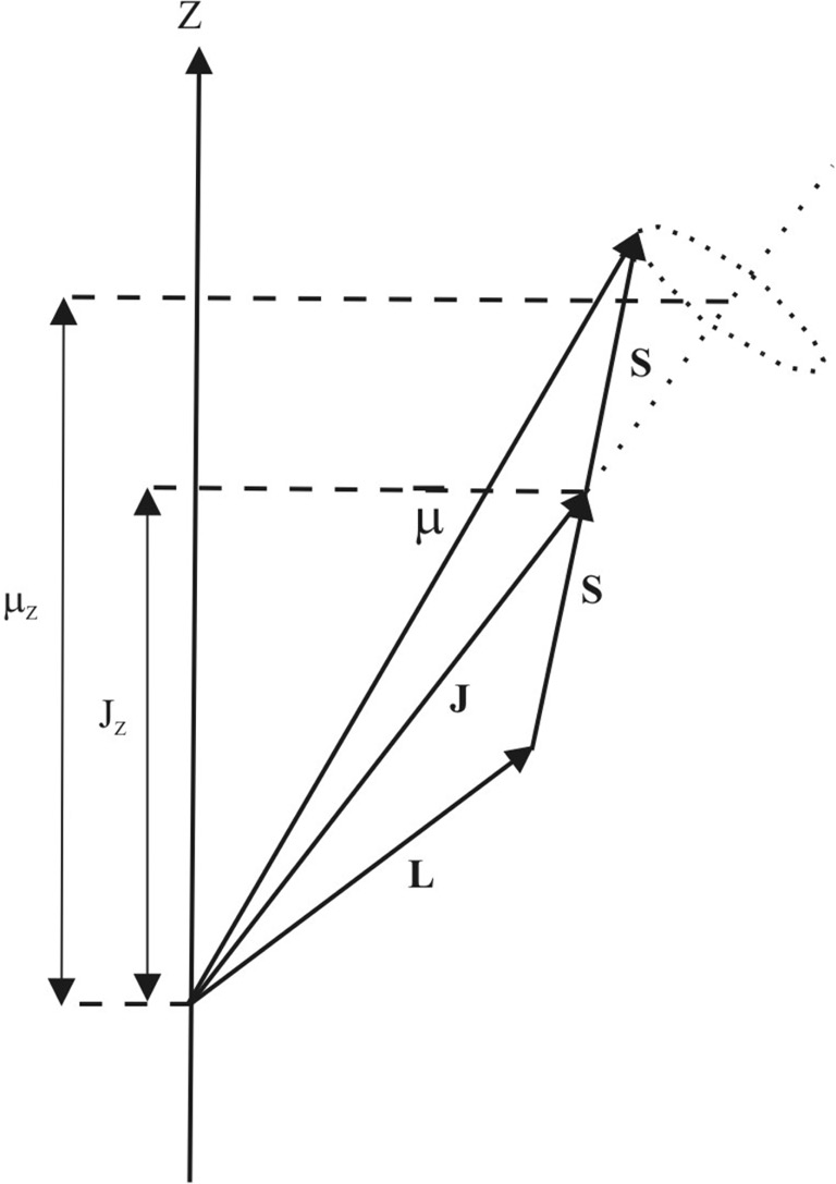
Figure 1.1 The relationship between angular momenta S, L and J and the magnetic moment μ as well as their projections J_z and μ_z along the z-axis.

Except for heavy atoms, the total orbital and spin angular momenta are related by Russell–Saunders coupling [12], governed by ℏL = ℏΣl and ℏS = ℏΣs. The resultant L and S then combine to give the total angular momentum J = L + S as in Figure 1.1. The z-components of J, m_J, may take any value from |L- S| to |L + S|, each (2J + 1)-fold degenerate, thus producing a multiplet in which the separation of the levels is determined by the spin-orbit coupling $\lambda L\cdot S$, where λ is the spin-orbit coupling constant. The values of S, L, and J for the lowest energy state are given by Hund’s rules, which are applied in the following sequence:

1. 1. S takes the maximum value permitted by the Pauli exclusion principle. Each subshell is given one “spin-up” electron before pairing it with a “spin-down” electron, starting from the lowest energy subshell (smallest m_𝓁 value).

2. 2. L takes the maximum value consistent with this value of S.

3. 3. For a half filled shell J = |L - S| and for a shell more than half full J = |L + S|.

Hund’s rules for electrons in d-orbitals (for which 𝓁=2 and m_𝓁 can take the values –2, –1, 0, 1, and 2) in doubly ionized Mn²⁺, Fe²⁺, Co²⁺, Ni²⁺, and Cu²⁺ (i.e. 3d⁵, 3d⁶, 3d⁷, 3d⁸, and 3d⁹) lead to the following angular momentum and magnetic moments shown in Table 1.1.

Table 1.1 Electronic configurations and effective Bohr magneton numbers p_J (total) and p_S (spin-only) for some doubly ionized elements.

	S	L	J	gJ	$p_J=g_J\sqrt{J\left(J+1\right)}$	$p_S=g_S\sqrt{S\left(S+1\right)}$	pexp
Mn2+	5/2	0	5/2	2	5.92	5.92	5.9
Fe2+	2	2	4	1.50	6.7	4.9	5.4
Co2+	3/2	3	9/2	1.33	6.63	3.87	4.8
Ni2+	1	3	4	1.25	5.59	2.83	3.2
Cu2+	1/2	2	5/2	1.20	3.55	1.73	1.9

It can be seen that the experimental effective Bohr magneton numbers (p_exp) are closer to the spin-only values (p_S). However, the situation becomes more complex when the atoms come together to form a solid. Since the 3d electrons are the outermost (valence) electrons, they can participate in the bonding. In ionic solids these electrons are perturbed by the inhomogeneous electric field E_c produced by neighboring ions (termed the crystal field or sometimes the ligand field), which breaks the coupling between L and S so that the states are no longer specified by J. Under the influence of the crystal field, the (2L + 1) degenerate orbital states in the free atom will be split. If this degeneracy is entirely lifted, then in a non-centrosymmetric field, the orbital angular momenta are no longer constant and may average to zero. This is conventionally called quenching of the orbital angular momentum (L = 0). However, in reality, the differences from the spin-only formula for the magnetic moment still arise from omitting the orbital angular momentum and spin-orbit coupling; hence, we can only really speak of partial quenching (L ≈ 0). A more detailed description is given in [14, 15].

If the neighboring ions are treated as point charges, which assumes no overlap or hybridization of their electron orbitals, then the crystal field (or ligand field) potential V_c satisfies Laplace’s equation, ${\nabla }^2{V}_c=-\nabla E_c=0$. Since the electric field $E_c=-\nabla V_c$, this implies that the gradient of the crystal field E_c is constant. Hence, the solutions are the Legendre polynomials, and the potential $V_c\left(r,\theta ,\phi \right)=\sum _l\sum _{m_l}{A}_l^{m_l}{r}^l{Y}_l^{m_l}\left(\theta ,\phi \right)$ can be expanded in spherical harmonics $Y_l^{m_l}\left(\theta ,\phi \right)$. The energy-level scheme and the occupation are governed by the symmetry of the crystal field, and the relative scales of the energies are given in Table 1.2. Note that the Coulomb interaction between the electrons and the atomic nucleus yields energy level spacings of the order of eVs, much larger than available thermal energies, which allows the total magnetic moment to be thermally stable. For an octahedral field, the five m_𝓁 states are split into two groups: a doubly degenerate e_g multiplet and a triply degenerate t_2g multiplet, which are separated by the crystal field energy Δ, with the latter multiplet being lower in energy, as shown in Figure 1.2. Their occupation depends on the relative importance of the energy Δ and spin-orbit energy λ(L·S). If Δ >> λ(L·S), Hund’s rules do not apply, and for Fe²⁺, the six d-electrons pair up and occupy the t_2g states producing S = 0. This represents the low-spin or strong-field configuration. For Δ << λ(L·S), the six electrons occupy the t_2g and e_g states in accordance with Hund’s rules, giving rise to the high-spin or weak-field situation.

Figure 1.2 The energy levels and associated orbitals of a d electron in an octahedral field split into a doubly degenerate e_g multiplet (d_x²_-y², d_3z²_-r²) and a triply degenerate t_2g multiplet (d_xy, d_yz, d_zx) separated by the crystal field energy Δ.

Table 1.2 Energy contributions as wavenumbers (spatial frequency of a wave in cycles per unit distance) associated with 3d ions, where 1 cm^–1 = 1.23984×10⁻⁴ eV. The Coulomb energy provides the ground state, the degeneracy of which can be lifted by the crystal field, the spin-orbit interaction or the Zeeman interaction in the presence of an applied magnetic field B = μ₀H in vacuum [17].

Coulomb energy	Crystal field	Spin-orbit	Zeeman
	Vc(r, θ, φ)	λ(L·S)	-gJμBmJB
10–40 × 103 cm–1	10–20 × 103 cm–1	100–800 cm–1	1 cm–1

If the overlap of the 3d wavefunctions between neighboring atoms is significant, then the electrons that carry the magnetic moments are delocalized (itinerant) and form continuous bands [16]. The magnetic electrons now participate in the conduction and their itinerancy can be characterized by the band width W, that is, the electrons spend a time t ~ ħ/W in the atom. Thus, the experimental moment values depend on the time constant of the technique used to determine them. The results given in Table 1.3 were obtained from magnetization, neutron diffraction, and X-ray magnetic circular dichroism (XMCD) measurements and represent time-averaged values. It is clear that moments arise predominantly from the spin and are non-integer, a feature explained by band theory. For example, the value for Ni is less than the fundamental unit of 1 μ_B. Electronic structure calculations have been carried out using different computational approaches and approximations for the exchange interaction describing coupling between spins (see Section 1.2.4.3 (Exchange Interactions)).

Table 1.3 Theoretical and observed magnetic moments given in μ_B [18]. The measured X-ray values are compiled from various references given in the reference section.

	μS(calc)	μL(calc)	μS(obs)neutron	μL(obs)neutron	μS(obs)X-ray	μL(obs)X-ray
Fe	2.21	0.06	2.13	0.08	2.246	0.051
Co	1.57	0.14	1.52	0.14	1.639	0.078
Ni	0.61	0.07	0.57	0.05	0.647	0.051

1.2.3 Macroscopic Considerations

In a solid, the periodic arrangement of atoms into a crystal (or lattice) can be described by the repetition of a unit cell containing a certain number of atoms (or chemical formula units) and characterized by a set of lattice parameters a, b, and c (for a cubic unit cell a = b = c). It is often more convenient to use the concept of reciprocal (or momentum) space, which correlates the unit real-space lattice vectors x, y, z by Fourier transformation into their reciprocal space counterparts $x\text{'},y\text{'},z\text{'}$ [17]:

$x\text{'}=2\pi \frac{y\times z}{x\cdot \left(y\times z\right)},y\text{'}=2\pi \frac{z\times x}{y\cdot \left(z\times x\right)},z\text{'}=2\pi \frac{x\times y}{z\cdot \left(x\times y\right)}\text{.}$(1.6)

The reciprocal space unit cell is called the Brillouin zone; for a simple cubic unit cell with a real-space lattice parameter a, the Brillouin zone is also simple cubic, with a reciprocal lattice parameter 2π/a.

The close proximity of the atoms in the lattice results in significant overlap (hybridization) of atomic orbitals of the outermost electrons, which will form continuous energy bands. The motion of the conduction electrons through the periodic energy landscape can be described using an ideal Fermi gas model, that is, a collection of non-interacting fermions. This motion can be described as a Bloch wave (momentum in a crystal). The Bloch wave has the form

$\psi \left(r\right)=u\left(r\right)e^{ik\cdot r},$(1.7)

where u(r) is a function with the same periodicity as the crystal and k is the crystal wavevector related to the crystal momentum p = ℏk. The components of k = (k_x, k_y, k_z) may be related to the real-space lattice vectors by a reciprocal-space transformation as shown in Eq. 1.6. Electrons described by Bloch waves behave almost as free particles in vacuum, just with a modified or effective mass m^*, as long as they reside in parabolic bands, that is, the dispersion relation is $E\left(k\right)=\frac{{\left(\hslash k\right)}^2}{2m^{*}}$.

For a collection of magnetic moments, for example, in a crystal, the macroscopic magnetization M is the net magnetic dipole moment per unit volume, defined as $M= \sum _i$, where μ_i is the time averaged atomic magnetic moment located on lattice site i. The sum is carried out over all lattice sites in the crystal. The magnetic induction (magnetic flux density) B is defined in terms of the torque Τ exerted on a dipole by a magnetic field: Τ = μ × B. The units are [N/Am], which can also be written as [Vs/m²], where the volt-second is the Weber (Wb) and so the units become Tesla [T]. The flux density and magnetization are related to the magnetic field H [A/m] through the equation B = μ_o(H + M), where μ₀ is the vacuum permeability with a value of ${\mu }_o=\frac{1}{{ϵ}_o{c}^2}=4\pi \times {10}^{-7}\left[\frac{Vs}{Am}\right]$. For a macroscopic sample, the magnetization is often linearly proportional to the applied field strength with the constant of proportionality being the magnetic susceptibility χ, M = χH. If the directional dependence becomes important, for example, in a single crystal, the full symmetry of the magnetic susceptibility tensor has to be considered: M $= \underset{\_}{\chi }B$. Without any additional assumptions, the tensor $\underset{\_}{\chi }$ is a 3 × 3 symmetric matrix with nine independent components. In general, the susceptibility is a tensor quantity and represents the temporal and spatial variation in M, that is, χ = χ(k,ω), where the angular frequency ω and magnitude of the wavevector k are given by the reciprocal relations ω = 2π/t and k = 2π/r. As will be discussed in Section 1.4.6, the susceptibility can be related to the neutron scattering function, and hence determined by neutron diffraction.

1.2.4 Calculation of Atomic Susceptibilities

The change in the energy of electrons located in an atom in a uniform magnetic field B is given by

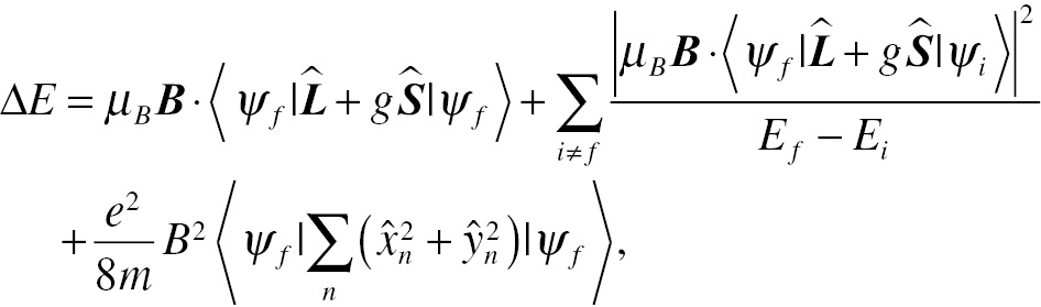$\begin{array}{c}\Delta E= {\mu }_{B}B\cdot 〈 {\psi }_f\text{|}\hat{L}+g\hat{S}\text{|}{\psi }_f〉+\sum _{i\ne f}\frac{{\left|{\mu }_{B}B\cdot 〈{\psi }_f\text{|}\hat{L}+g\hat{S}\text{|}{\psi }_i〉\right|}^2}{E_f-E_i}\\ +\frac{e^2}{8m}{B}^2〈{\psi }_f\text{|}\sum _n\left({\hat{x}}_n^2+{\hat{y}}_n^2\right)\text{|}{\psi }_f〉,\end{array}$(1.8)

where E_f is the final state (ψ_f) energy, E_i is the initial state (ψ_i) energy, e and m are the charge and mass of the electron, respectively, and ${\hat{x}}_n,{\hat{y}}_n$ are position operators defining its spatial coordinates. From this equation, the magnetization and susceptibility can be calculated.

1.2.4.1 Diamagnetism

Based on an atomic application of Lenz’s law, which states that a current loop induced by a changing magnetic field produces a magnetic moment, which opposes the applied field, a diamagnetic susceptibility is always negative. All materials show a diamagnetic response but the weakness of the effect means that it is only measurable in the absence of any other magnetic behavior.

For atoms with closed shells, such as He, Ne, and Ar, there is no net spin or orbital angular moment following Hund’s rules. Hence, there is no permanent magnetic moment located on the atom, and for the ground state ψ_0, the expectation values of the orbital and spin angular momentum operators $〈{\psi }_0\text{|}\hat{L}\text{|}{\psi }_0〉= \sqrt{L(L+1)}$ and $〈{\psi }_0\text{|}\hat{S}\text{|}{\psi }_0〉=\sqrt{S(S+1)}$ are both zero. The applied magnetic field produces a flux density B, which in turn causes a screening current to flow and so the magnetization M is obtained from $M\left(B\right)=-\frac{1}{V}\frac{\partial E_o\left(B\right)}{\partial B}$ and the susceptibility from $\chi ={\mu }_o\frac{\partial M\left(B\right)}{\partial B}=-\frac{{\mu }_o}{V}\frac{{\partial }^2{E}_o\left(B\right)}{\partial B^2}$. The Larmor diamagnetic susceptibility is negative and has the form

${\chi }_{Larmor}=-{\mu }_0\frac{N}{V} \frac{{\partial }^2\Delta E_0\left(B\right)}{\partial B^2}= -{\mu }_0\frac{N}{V}\frac{e^2}{6m}〈{\psi }_0\left|\sum _i{\hat{r}}_i^2\right|{\psi }_0〉,$(1.9)

where N is the number of atoms or ions and V the volume. Magnetic susceptibilities are often quoted as molar susceptibilities, based on the magnetization per mole rather than per volume. The conversion is made by multiplying the volume susceptibility by the factor $\frac{N_A}{\left(N/V\right)}$, where N_A = 6.02214086 × 10²³ is Avogadro’s constant. The expectation value $〈{\psi }_0\left|\sum _i{r}_i^2\right|{\psi }_0〉$ is the square of the most probable radius of the outermost electron shell and can only be properly evaluated by a full quantum-mechanical treatment. However, we can make estimates of the electron shell radius by various means. From semi-classical models of the hydrogen atom, the most probable distance between the proton and the electron can be defined as the Bohr radius a₀ = 0.529 Å. For ions of substances like the alkali halides (e.g. F, Br, and Cl) or the solid forms of the noble gases, the mean square ionic radius can be defined as $〈r^2〉=\frac{1}{Z}〈{\psi }_0\left|\sum _i{r}_i^2\right|{\psi }_0〉$, where Z is the atomic number (the total number of electrons in the atom or ion), and <(r/a₀)²> is of order unity. However, for metals, as the electrons are delocalized, a commonly used measure is the free electron radius r_s, which is the radius of a sphere the volume of which is equal to the volume per conduction electron. If the sample of interest has atomic mass A and mass density ρ_m, the number of moles per cubic metre is ρ_m/A (if ρ_m is given in grams per m³). There are N_A atoms per mole and if each atom contributes Z_i conduction electrons, there are (N_AZ_iρ_m)/A conduction electrons per unit volume (in m³). As each conduction electron occupies a sphere of volume (4πr_s³)/3, r_s is therefore given by

$\frac{4\pi r_s^3}{3}=\frac{A}{N_A{Z}_i{\rho }_m} \Rightarrow r_s= {\left(\frac{3A}{4\pi N_A{Z}_i{\rho }_m}\right)}^{\frac{1}{3}}.$(1.10)

Examples of diamagnets are (solid) noble gases, simple ionic crystals, such as alkali halides, graphite, many good metallic conductors (superconductors are perfect diamagnets as they offer no resistance to the formation of current loops), and a number of substrate materials, for example, GaAs. To a first approximation, the contributions of the various ions add for the halides.

Table 1.4 Diamagnetic susceptibility of some materials around 293 K ${\chi }_{diamag}^{molar}$ in (10^–6 cm³ mol^–1) [19, 20, 21].

Cu	Ag	Au	Si	Ge	Graphite	B	SiC	SiO2	Al2O3	GaAs	GaN
–5.46	–19.5	–28	–3.12	–11.6	–6.0	–6.7	–12.8	–29.6	–37	–33.15	–34.9

Note that, in general, the magnetic susceptibility of conduction electrons is composed of several contributions that are difficult to separate experimentally. For metallic solids, there are two different ‘sources of diamagnetism’, namely the filled electronic shells of the ions (these give rise to the Larmor diamagnetism, as discussed above) and the diamagnetic contribution of the free conduction electrons (which give rise to Landau diamagnetism). The angular momentum in a plane perpendicular to the applied magnetic field is quantized, giving rise to a set of discrete energy levels. The statistical thermal occupation of these Landau levels gives rise to the Landau susceptibility:

${\chi }_{Landau}=-\frac{2}{3}\rho \left(E_F\right){\mu }_B^2{\left(\frac{m}{m^{*}}\right)}^2,$(1.11)

where ρ(E_F) is the density of states (DOS) at the Fermi energy E_F and the last term accounts for the fact that the Bohr magneton is defined for free electrons, rather than those in a band. The Fermi energy is the energy difference between the highest and lowest occupied single particle states at 0 K, and for a metal, it is the energy difference between the Fermi level and the bottom of the conduction band. Except for very low temperatures and high magnetic fields, at which the de Haas–van Alphen effect (oscillations of the magnetic moment in a metal with magnetic field) may be observed, χ_Landau is essentially temperature independent.

1.2.4.2 Paramagnetism

The metallic elements that are paramagnetic have a weakly temperature-dependent susceptibility, but in contrast to diamagnets, it is positive (M increases with H) [22]. In the Hartree–Fock approximation, the susceptibility is given by the occupation of the electronic states: ${\chi }^p=\frac{g_J^2{\mu }_B^2}{V}\sum _k\frac{f_{dk-}{f}_{k+dk}}{E_{k+dk}-E_k}$, where the sum runs over all wavevectors k and considers the effect on the occupation probability f and energy E of a small variation dk. At T = 0 K, assuming a parabolic energy momentum relation (as in Section 1.2.3), this expression reduces to the Pauli susceptibility:

${\chi }_o^p= \frac{g_J^2{\mu }_B^2}{2}\rho \left(E_F\right)\text{and}\rho \left(E_F\right)=\frac{3N}{2E_F} ,$(1.12)

which results from the Zeeman splitting, which is a relative shift in the conduction band for spin-up and spin-down electrons in an applied magnetic field. Since the Fermi level must be the same for both subbands, there will be a surplus of electrons in one of them and hence a net spin polarization. The variation at finite temperatures depends on the details of the DOS at the Fermi energy. At temperature T, the DOS $\rho \left(E\right)$ must now be multiplied by the Fermi function: $f\left(E\right)= \frac{1}{1+e^{\frac{\left(E-E_F\right)}{k_{B}T}}}$, which gives the statistical occupation of the electronic states at energy E. The room temperature paramagnetic susceptibility of some relevant elements is given in Table 1.5.

Table 1.5 Observed paramagnetic susceptibility of some transition metals around 293 K ${\chi }_{para}^{obs}$ in (10^–4 cm³ mol^–1) [19].

Zr	Nb	Ru	Rh	Pd	Hf	Ta	W	Pt
1.2	2.08	0.39	1.02	5.4	0.71	1.54	0.53	1.93

There is yet another contribution to the paramagnetic susceptibility, which is the temperature-independent Van Vleck paramagnetism. If the ground state of the system, ψ₀, hybridizes with an excited state, ψ_e, separated from it in energy by Δ, and $\Delta \gg k_{B}T$, then the contribution can be written as ${\chi }_{VV}= \frac{2N{\left|〈{\psi }_e|{\hat{\mu }}_z|{\psi }_0〉\right|}^2}{\Delta }$, where N is the number of atoms per unit volume and ${\hat{\mu }}_z$ is the magnetic moment operator projected onto the z-axis (the assumed magnetic field direction).

1.2.4.3 Ferromagnetism and Antiferromagnetism

Susceptibility of Local Moments

A collection of N identical atoms per unit volume with total angular momentum J in an applied field B = μ₀H has a magnetization $M=N{g}_J{\mu }_{B}J{B}_J\left(x\right)$, where $x=\frac{g_J{\mu }_{B}JB}{k_{B}T}$ is the ratio between Zeeman and thermal energies, and B_J(x) the Brillouin function (see Eq. (1.14)), which was tabulated for different J values in [23]. In the classical limit, J→$\infty$, it approaches the Langevin function used in the analysis of superparamagnets:

$L\left(x\right)=\coth x-\frac{1}{x},$(1.13)

For $x\ll 1,$

$B_J\left(x\right)=\frac{2\text{J}+1}{2\text{J}}\coth \frac{2\text{J}+1}{2\text{J}}x-\frac{1}{2\text{J}}\coth \frac{1}{2\text{J}}x\cong \frac{\text{J}+1}{3\text{J}}x$(1.14)

$\Rightarrow M=\frac{N{\mu }_B^2{g}_J^{2}J\left(J+1\right)}{3k_{B}T}B.$(1.15)

The susceptibility then becomes

$\chi =\frac{M}{H}=\frac{{\mu }_{0}N{\mu }_B^2{g}_J^{2}J\left(J+1\right)}{3k_{B}T}=\frac{\text{C}}{\text{T}},$(1.16)

where C is the Curie constant. Plotting the inverse of $\chi$ against temperature yields a straight line passing through the origin, with slope C^–1. This allows the effective paramagnetic moment ${\mu }_{eff}=\sqrt{\frac{3k_{B}C}{{\mu }_{0}N{\mu }_B^2}}$ to be compared to the theoretical value, ${\mu }_{eff}=g_J\sqrt{J\left(J+1\right)}$.

Allowing interaction between the moments leads to a phase transition and a cooperative ground state, the nature of which depends on the details of the interaction. Using a mean field approach (first introduced as the Weiss molecular field), the interaction is assumed to be an internal field H_int proportional to the magnetization M, where H_int = λM and λ is independent of temperature. Above the transition temperature T_C the induced magnetization is M = χ(H + H_int), and so MT = C(H + λM) and

$\chi =\frac{M}{H}=\frac{C}{\left(T-C\lambda \right)}.$(1.17)

Figure 1.3 The thermal variation of the inverse susceptibility for a system of non-interacting local moments (Curie paramagnet) and for the mean field approximation (Curie–Weiss paramagnet).

This is the Curie–Weiss law (see Figure 1.3). It indicates that a plot of χ^–1 versus T will give an intercept at a temperature T_C, sometimes referred to as the Weiss constant or the paramagnetic Curie temperature. When T = T_C = Cλ, the susceptibility χ is singular. The value of the mean field constant λ can be obtained from the Curie constant:

$\lambda =\frac{T_C}{C}=\frac{3k_B{T}_C}{{\mu }_{0}N{g}_J^{2}J\left(J+1\right){\mu }_B^2}.$(1.18)

For example, for bulk iron, T_C = 1043 K, g_J = 2, and J ~ S = 1 gives λ ~ 589. With a saturation magnetization M_s (at 0 K) = 1752 emu·cm^–3 = 22016 G, H_int ~ 13 x 10⁶ G (10⁴ G ≡ 1T). Thus, this ‘internal field’ H_int is very much larger than the magnetic field produced by neighboring moments, which can be estimated as μ_B/a³ ~ 5309 G, where a = 0.28 nm is the lattice parameter of iron. From this analysis, it becomes clear that the magnetism in materials such as iron cannot arise from a classical picture of interacting magnetic dipoles.

Exchange Interactions

Ferromagnets, such as Fe, require an additional phenomenon that causes the magnetic moments to align in parallel spontaneously below T_C, even in the absence of an applied magnetic field. We can explain this behavior by first introducing an exchange integral, J^ex, related to the charge distributions of two atoms on different lattice sites i and j, each with uncompensated spins. The Pauli exclusion principle introduced earlier dictates that the charge distribution of a system of two spins depends on whether the spins are parallel or antiparallel. Hence, the electrostatic energy of a system depends on the relative orientation of the spins. The difference in energy between the two cases defines the exchange energy.

The coupling between localized spins, on different lattice sites i and j, which gives rise to cooperative phenomena is usually mediated by the ‘Heisenberg’ exchange mechanism described by the Hamiltonian:

${\hat{H}}_{Heis}=-2\sum _{i\ne j}{J}_{ij}^{ex}{s}_i\cdot s_j,J_{ij}^{ex}=\{\begin{array}{c}{J}^{ex},\text{if}i\text{and}j\text{are}\text{neighbors}\\ 0,\text{otherwise}\end{array},$(1.19)

where $J_{ij}^{ex}$ is the exchange constant between two spins s_i and s_j. Although originally derived for localized moments using the Heitler–London approximation [17], it is generally also applied to metallic systems. The exchange interaction can be positive, $J_{ij}^{ex}>0$, or negative, $J_{ij}^{ex}<0$, giving rise to parallel (ferromagnetic, FM) or antiparallel (antiferromagnetic, AF) alignment of the spins. Ferrimagnetism occurs if two ferromagnetic sublattices of unequal moments are coupled antiferromagnetically. An estimate of the strength of the interactions is given by the transition temperatures, known as the Curie temperature T_C for ferromagnets, which for Fe, Co, and Ni are 1043, 1395, and 633 K, respectively, and the Néel temperature T_N for antiferromagnets, which for Cr and NiO are 311 and 513 K, respectively. Again, these values are considerably higher than those predicted on the basis of pure dipole-dipole interactions, for which the Hamiltonian has the form

${\hat{H}}_{dip}=\frac{{\mu }_0}{4\pi }\left(\frac{{\mu }_i\cdot {\mu }_j}{r_{ij}^3}-3\frac{\left({\mu }_i\cdot r_{ij}\right)\left({\mu }_j\cdot r_{ij}\right)}{r_{ij}^5}\right),$(1.20)

where r_ij is the separation between magnetic moments μ_i and μ_j located at positions r_i and r_j. By using Eq. (1.17), this interaction yields transition temperatures of the order of only 1 K.

We can estimate the relation between J_ex and T_C through the gain in potential energy of the magnetic moment μ_j in the magnetic field H_i produced by the moment μ_i as

$E= -{\mu }_j\cdot H_i=-2\left(\frac{1}{2}{\text{g}}_{\text{s}}^2{\mu }_{\text{B}}^2\lambda \right)s_i\cdot s_j$(1.21)

$\Rightarrow J^{ex}=\frac{3k_B{T}_c}{2nS(S+1)},$(1.22)

where now n represents solely the number of the nearest neighbors, each connected with the central atom j by J^ex (for all other atoms J^ex =0).

The shortcoming of this model lies in its assumption that the interacting electrons are strongly localized to the atoms, so it does not accurately describe ferromagnetism in materials such as Fe, Co, and Ni, where the magnetic moment-carrying electrons are delocalized in the conduction band. Predictions of the Curie temperature T_C and J^ex given by Eq. (1.22) above are either of the wrong sign or too small. For those cases, a better model was proposed by Edmund Stoner that takes into consideration the band structures of the materials.

Here the bands are spontaneously split into two subbands depending on their spin-orientation. The energy dispersion relation is now spin-dependent and can be expressed as

$E_{\uparrow }\left(k\right)=E_0\left(k\right)- I\frac{n_{\uparrow }-n_{\downarrow }}{n_{\uparrow }+n_{\downarrow }},$(1.23)

$E_{\downarrow }\left(k\right)=E_0\left(k\right)+ I\frac{n_{\uparrow }-n_{\downarrow }}{n_{\uparrow }+n_{\downarrow }},$(1.24)

where E₀(k) is the unperturbed band, n_↑ and n_↓ are the number of spin-up and spin-down electrons, and I the Stoner parameter. The parameter is defined as I = Δ/μ, where Δ is the difference in energy between the spin-up and spin-down bands, and μ the magnetic moment in units of μ_B per atom. The condition for ferromagnetism, that is, the spin polarization $P=\frac{n_{\uparrow }-n_{\downarrow }}{n_{\uparrow }+n_{\downarrow }}\ne 0$, is then given by the Stoner criterion:

$I\tilde{\rho }\left(E_F\right)>1,$(1.25)

where $\tilde{\rho }\left(E_F\right)= \frac{\rho \left(E_F\right)}{2N}$ is the density of states per atom per spin orientation at E_F. Usually, s and p electrons are delocalized, 4f electrons are localized, and 5f and 3d/4d electrons are somewhere in between. In materials with contributions to the magnetic interaction from both delocalized and localized electrons (e.g. Gd), the Ruderman–Kittel–Kasuya–Yosida (RKKY) model is the currently accepted mechanism.

In this model, which accounts for an indirect exchange mechanism, the localized moment (e.g. of the Gd 4f electrons), polarizes the electrons in the 6s/5d hybridized conduction band, which then couple to more distant moments. Assuming that g_J = 2, the exchange is given by [17]

$J_{RKKY}\left(R\right)=-\frac{9\pi }{8}\frac{J_0^2}{E_F}\frac{\left(2k_{F}R\right) \cos \left(2k_{F}R\right)-\text{ sin}\left(2k_{F}R\right)}{{\left(2k_{F}R\right)}^4},$(1.26)

where R is the distance between localized (l) and itinerant electron (i), k_F is the wavevector at the Fermi energy, and J₀ is the exchange integral between localized and itinerant electron wavefunctions at zero momentum transfer, that is, q = k_l – k_i = 0. From Eq. (1.26), we see that the exchange oscillates between AF and FM coupling, and the amplitude decreases rapidly with increasing distance (see Chapter 6, Section 6.2.1.2).

Indirect exchange interaction can also give rise to helical magnetic order, such as in the rare-earth element Eu, while in insulating compounds, such as NiO and MnO, it usually gives rise to antiferromagnetism. Depending upon the crystal structure, both cation-cation and cation-anion-cation interactions can occur. For superexchange interaction, the wavefunctions of the outermost electrons on the cation admix with those on the anion, thus enabling two cations to couple indirectly. For example, in NiO, superexchange arising from hybridization between 3d Ni²⁺ and 2p O^2– states leads to AF order. An extension of the model, double exchange, was proposed to account for transport properties in compounds such as the ferrimagnet Fe₃O₄ (magnetite) in which the cations have two different valencies, that is, Fe³⁺ and Fe²⁺. In contrast to superexchange, where the electrons remain in their respective ions, in double exchange they can move between the two cations through the intermediate anion, giving rise to metallic conductivity.

Magnons

We can also use the mean field approach as introduced in Sections 1.2.1 and 1.2.4.3 (Susceptibility of Local Moments) to describe the temperature dependence of the saturation magnetization M_s of a ferromagnet below T_C. However, this time we need to use the whole expression for the Brillouin function B_J(x) as given in Eq. (1.14), remembering that the magnetization is given by M = Ng_Jμ_BJB_J(x). For J = S =1/2 and g_J = 2, we have $M_s=N{\mu }_B\tan h\left(\frac{{\mu }_{B}B}{k_{B}T}\right)=N{\mu }_B\tan h\left(\frac{{\mu }_B\lambda M}{k_{B}T}\right)$, if we assume the magnetic field B to be solely the internal field H_int, which can be solved numerically for 0 ≤ T ≤ T_c. As the temperature increases, the magnetization smoothly decreases and vanishes completely at T_C, reminiscent of a second-order phase transition from a ferromagnetic to a paramagnetic state.

The decrease of the saturation magnetization with increasing temperature is driven by the thermal excitations (spin waves). In the simplest model, one can picture a one-dimensional chain in which all the spins are ferromagnetically aligned, except for one spin that has been flipped. As the spin is quantized (up or down), so is the excitation, which is termed a magnon. The exchange energy as described by the Heisenberg model in Eq. (1.19) to completely reverse a single spin amounts to 8J^exS², which is relatively high. The energy of the excitation can be considerably reduced by spatially distributing the magnon through a continuous gradual rotation of the magnetic moments of many neighboring spins in the chain. This gives the magnon a continuous wavelike character.

In localized antiferromagnets or ferromagnets, which can be approximated by the Heisenberg model, magnons propagate through the Brillouin zone with a dispersion relation (the dependence of the angular frequency ω on the crystal momentum k) given by

$\hslash \omega \left(k\right)= 4J^{ex}S\left(1-\cos ka\right) \approx \left(2J^{ex}S{a}^2\right)k^2$(1.27)

for a ferromagnet, where a is the lattice constant and D = (2J^exSa²) is the spin wave stiffness constant, and

$\hslash \omega \left(k\right)= 4S\left|J^{ex}\sin ka\right| \approx 4S{J}^{ex}ak$(1.28)

for an antiferromagnet. In both cases, the approximation assumes ka « 1, that is, the wavelength is large compared to a.

In the Heisenberg model, the transition from the ferromagnetic to paramagnetic phase is driven by transverse fluctuations of the moment, with its magnitude remaining fixed. This is in contrast to the Stoner model in which the paramagnetic phase is driven by amplitude fluctuations, with the moment decreasing as the temperature increases until it vanishes at T_C.

1.3 Magnetization Processes

1.3.1 Magnetic Anisotropies

In single crystalline ferromagnets, the magnetization depends on the magnitude and direction, with respect to the crystallographic axes, of the externally applied magnetic field. This gives rise to easy and hard directions of magnetization (the anisotropy being greater the lower the crystal symmetry). The origin of this magneto-crystalline anisotropy is the spin-orbit interaction. For cubic crystals, for example, body-centered cubic (bcc) Fe, and face-centered cubic (fcc) Ni, the anisotropy energy density, E_K, is usually expressed in terms of the directional cosines α_i, which are the cosines of the angles between the magnetization M and the three crystallographic axes x, y, z, namely

$E_K= K_o+ K_1\left({\alpha }_1^2{\alpha }_2^2+ {\alpha }_2^2{\alpha }_3^2+ {\alpha }_3^2{\alpha }_1^2\right)+ K_2\left({\alpha }_1^2{\alpha }_2^2{\alpha }_3^2\right)+\text{higher order terms}\text{.}$(1.29)

The magneto-crystalline anisotropy constants K_i can be obtained from magnetization measurements using single crystals by making use of the work done in the magnetization process $\underset{0}{\overset{M_s}{\int }}H\cdot dM$, which represents the area between M = M_s and the magnetization curve for the crystallographic direction of interest. If the third term is zero, then the easy axes are <100> for K₁ > 0 (as for Fe) and <111> for K₁ < 0 (as for Ni). For uniaxial systems, for example, hexagonal closed packed (hcp) Co, the expression in polar coordinates becomes

$E_K= K_o+ K_{1}si{n}^2\theta + K_{2}si{n}^4\theta +\text{higher}\text{order}\text{terms},$(1.30)

where θ is the angle between the magnetization and the hexagonal axis. If K₁ = K₂ = 0, the magnetization is isotropic. For K₁ > 0 and K₂ > –K₁, the easy axis of magnetization is the hexagonal axis and for K₁ > 0 and K₂ < –K₁, it is fixed in the basal plane. In all cases, K₀ is chosen to make E_K zero along the easy axis. Some measured values of the magneto-crystalline anisotropy constants for Fe, Co, and Ni are given in Table 1.6.

Table 1.6 Magneto-crystalline anisotropy constants.

	K1 × 104Jm–3	K2 × 104Jm–3
Fe (4.2K)	4.8	± 0.5
Ni (4.2K)	−0.50	−0.20
Co (300K)	45.0	15.0

The values decrease with increasing temperature, vanishing at T_C. The variation is predicted [24] to be

$\frac{K_1\left(T\right)}{K_1\left(0\right)}= {\left[\frac{M\left(T\right)}{M\left(0\right)}\right]}^{\delta },$(1.31)

where δ = 3 or 10 for uniaxial and cubic ferromagnets, respectively.

Nanoparticles or films in the ultrathin limit of a few nms are usually assumed to have a uniaxial crystalline anisotropy given by

$E_B= K_{u}V{\sin }^2\theta .$(1.32)

Figure 1.4 A representation of the energy of a uniaxial magnetic nanoparticle as a function of the direction of the magnetization. The height of the barrier E_B characterizing the thermally induced magnetization reversal is given by KV, where K is the magnetic anisotropy constant and V the particle volume. Changes in the energy landscape in the (a) absence and (b) presence of an applied external magnetic field are indicated schematically.

This has minima at θ = 0 and π that are separated by an energy barrier E_B of height K_uV, as shown in Figure 1.4. However, other types of anisotropy may dominate. Classically, the magnetization must overcome this energy barrier to reverse, although the possibility of quantum mechanical tunneling has also been considered [25]. When a ferromagnet or ferrimagnet is placed in a magnetic field, magnetic poles of opposite signs are induced at the ends of the specimen and a demagnetizing field is established that opposes the direction of the externally applied field. The demagnetizing field is responsible for the magnetostatic energy, which depends on the direction of the magnetization and the shape of the specimen, which is why it is also termed the shape anisotropy. For a prolate spheroid with the semi-major axis c and the semi-minor axes a = b, the magnetostatic energy is given by

$E_{shape}= \frac{1}{2}{\mu }_o{M}_s^{2}V\left(N_a-N_c\right)si{n}^2\theta ,$(1.33)

where N_a and N_c are demagnetization factors in the a and c directions, and θ is the angle between the magnetization and the c axis. For spheres, N_a = N_c and E_shape = 0, but for non-spherical particles, E_shape can be significantly larger than the magneto-crystalline anisotropy.

In addition, magneto-elastic anisotropy occurs when strains in the specimen give rise to a non-uniform structure. The strains may arise during fabrication via defects or dislocations, epitaxial growth on a substrate with a different lattice constant, or can be purposely externally applied, for example, with a pressure cell. The magnetization process gives rise to magnetostriction with an associated energy, which for an isotropic system is given by

$E_{strain}=-\frac{3}{2}{\lambda }_s\sigma co{s}^2\theta ,$(1.34)

in which λ_s is the saturation magnetostriction, σ is the stress, and θ the angle between the magnetization and the strain.

Exchange (bias) anisotropy occurs when a sample containing an interface between a ferromagnet and an antiferromagnet is cooled below the antiferromagnet’s Néel temperature T_N, where the T_C of the ferromagnet is significantly higher than T_N. This was originally observed in ferromagnetic Co particles covered by a shell of AF CoO [26]. When the cooling takes place in a magnetic field, an exchange bias occurs, in which the magnetization versus applied field curve (M-H loop or hysteresis loop) is displaced along the field axis in the direction that opposes the applied field. An increased coercivity (or coercive field, the applied field required to reduce the total magnetization to zero) is also observed after cooling, which disappears together with the exchange bias as T_N is approached.

1.3.2 Magnetic Domains

The magnetization process of a ferromagnet is shown in Figure 1.5. In the virgin state and in the absence of an applied field, the macroscopic magnetization is generally significantly less than maximum saturation owing to the presence of domains. Within each domain, the magnetization is saturated, but its direction in neighboring domains is different. The domain structure [27] can be imaged using Bitter patterns, optically using Faraday or Kerr rotation, XMCD photoemission electron microscopy (PEEM) [28, 29] or, more recently, magnetic force microscopy (MFM) [30, 31]. Similarly, upon cooling below the Néel temperature, AF domains emerge. AF domains have been extensively studied using neutron diffraction [32], X-ray and neutron diffraction topography [33], and X-ray magnetic linear dichroism (XMLD) PEEM [34].

Figure 1.5 The magnetization M as a function of field H for a (a) superparamagnet, (b) soft ferromagnet, and (c) hard ferromagnet. H_c, H_K, M_R, and M_s are the coercive field, the anisotropy field, the remanence and the saturation magnetization, respectively.

From neutron scattering, it is known that upon entering an ordered magnetic phase, additional diffraction peaks emerge that are not present in the paramagnetic phase, such as the (½,½,½) peak of NiO presented in Figure 1.6. The reason for this is that the magnetic lattice has a lower symmetry than the crystal lattice (which can represent the pure paramagnetic phase), adding a new degree of freedom to the system to lower its total magnetostatic energy by breaking up the magnetic phase into domains. In terms of symmetry groups, if the order of the paramagnetic group is p and that of the magnetic group is m, then the number of different domains will be p/m.

Figure 1.6 The nuclear (2 2 0) peak at 550 K and the AF magnetic (½½½) peak at 5 K with Gaussian fits convoluted with the instrument resolution function used to determine the particle and magnetic sizes.

Magnetic domains can be classified into the following groups depending on the symmetry lost upon magnetic ordering:

1. 1. configuration domains – translational symmetry;

2. 2. 180° domains – time inversion symmetry;

3. 3. orientation domains – rotational symmetry; and

4. 4. chirality domains – centrosymmetry.

Configuration domains occur whenever the propagation vector τ in reciprocal space describing the magnetic structure is not transformed into itself or itself plus a reciprocal lattice vector by all the symmetry operators of the paramagnetic group. The presence of 180° domains in a crystal implies that τ = 0 and the directions of the magnetic moments in one domain are reversed with respect to corresponding moments in the other and hence, the perpendicular magnetization is reversed. Orientation domains occur when the magnetic space group is not congruent with the group describing the configurational symmetry, that is, the magnetic configuration from one domain into another cannot be transformed through rotation. If the paramagnetic space group is centro-symmetric, for example, bcc, but the magnetic structure is not, then chirality domains can occur [35].

1.3.2.1 Domain Walls

The transition region between neighboring domains is known as a domain wall, over which the magnetization continuously changes from its value in one domain to that in the other. Similar to the spin wave argument (Section 1.2.4.3 (Magnons)), the entire rotation of the magnetization between domains takes place gradually over many atomic planes, as the exchange energy is lower when the change is distributed over many spins. For a Bloch wall, the magnetization rotates out of the plane defined by the magnetizations of the two domains (Figure 1.7) and is thus most common in ferromagnetic bulk samples or thick films.

Figure 1.7 Schematic depicting (a) a Néel and (b) a Bloch domain wall within the box.

The width δ_dw of the wall separating neighboring 180° (π) domains is governed by contributions from both the exchange interaction J^ex and the magnetic anisotropy K, which prevents the domain wall from extending over the whole sample, and is given by [11]:

${\delta }_{dw}=\pi {\left(\frac{A}{K}\right)}^{\frac{1}{2}}=\pi {\left(\frac{N{J}^{ex}{S}^2}{Ka}\right)}^{\frac{1}{2}},$(1.35)

where a is the length of the side of the unit cell and A is the exchange stiffness constant given by

$A=\frac{N{J}^{ex}{S}^2}{a},$(1.36)

where N is the number of atoms per unit cell. For bcc Fe, J^ex = 2.16 × 10^–21 J, S = 1, a = 2.9 × 10^–10 m and N = 2, so that A = 1.49 × 10^–11 Jm^–1. Measured values of A for Co, Ni, and Fe as determined by spin-wave resonance [17] are shown in Table 1.7. Typically, δ_dw is of the order 30 nm in Fe at room temperature (around 100 unit cells). The energy stored in the domain wall is given by

$E_{dw}=2\pi {\left(AK\right)}^{\frac{1}{2}}=2\pi {\left(\frac{N{J}^{ex}{S}^{2}K}{a}\right)}^{\frac{1}{2}}.$(1.37)

Table 1.7 Measured exchange stiffness constants [17].

	A × 10–11 Jm–1
Fe (295K)	2.5
Ni (295K)	0.75
Co (295K)	1.3
Co (4K)	1.43

Under the application of a magnetic field, the volumes of domains whose directions are closest to that of the field reversibly increase. Owing to crystal imperfections, this growth becomes irreversible at higher fields with the magnetization finally rotating into the field direction. The overall process gives rise to hysteresis, as shown in Figure 1.5. The ratio of the remanence M_R (the remanent magnetization after saturation in the absence of any applied field) over the saturation magnetization M_s is often used to indicate the ‘squareness’ of the hysteresis when assessing materials and optimizing their hysteresis for particular technical applications. For example, permanent magnets require a high coercive field H_c and remanence M_R, whereas transformers need a narrow hysteresis to reduce energy loss $\oint MdH$ (the area enclosed by the hysteresis loop) as afforded by the high relative permeability μ_r in soft ferromagnets. Note that the relation between B and H in vacuum is thus modified to B = μ_rμ₀H in a medium.

As the magnetic configuration is governed by exchange on the short scale and dipolar energy at a larger scale, the competition between these energies results in a characteristic distance below which exchange dominates and above which magnetostatic interactions dominate. This very important distance is the length scale over which the perturbation due to the switching of a single spin decays in a soft magnetic material, and is termed the ferromagnetic exchange length [36]:

$L_{ex}=\sqrt{\frac{A}{{\mu }_o{M}_s^2}},$(1.38)

which represents the ratio between the square roots of the exchange energy and the magnetostatic energy, and is typically 3 nm in Fe- and Co-based alloys. Whether a material is considered magnetically ‘hard’ or ‘soft’ is defined by a dimensionless parameter κ, the ratio of L_ex and δ_dw:

$\kappa =\frac{\pi L_{ex}}{{\delta }_{dw}}=\sqrt{\frac{K}{{\mu }_o{M}_s^2}}.$(1.39)

For hard magnetic materials, κ approaches unity, whereas it tends to zero for soft ferromagnets.

1.3.2.2 Magnetization Reversal

Magnetization Reversal in Thin Films and Particles

As the dimensions of the specimen are reduced, the energy required to form a domain wall becomes greater than the reduction in magnetostatic energy as indicated by L_ex. As a result, for thin films whose thickness approaches that of the domain wall width, a different type of wall, a Néel wall [37], is established in which the magnetization rotates within the plane defined by the magnetizations of the two domains (Figure 1.7). Eventually, with further reduction in dimensions, a particle will form that consists of a single domain. For a particle with uniaxial anisotropy K_u, the critical radius r_c for this to occur is [11]:

$r_c=\frac{9E_{dw}}{2{\mu }_o{M}_s^2}=9\pi \kappa L_{ex}=\frac{9\pi \sqrt{A{K}_u}}{{\mu }_o{M}_s^2}.$(1.40)

Values for the critical diameter d_c and domain wall energy E_dw of various ferro- and ferri-magnetic materials are given in Table 1.8. Depending on the material, the critical radius lies in the range 2.5–500 nm.

Table 1.8 Critical diameter d_c and domain wall energy for Fe, Co, Ni, γ-Fe₂O₃, and Fe₃O₄ [1, 38].

	dc [nm]	Edw [mJ/m2]
Fe	14	3
Co	70	8
Ni	55	1
γ-Fe2O3	166
Fe3O4	128

Figure 1.8 Log₁₀-log₁₀ plot of the coercivity H_c versus grain size d for several soft magnetic systems. ■ permalloy, □ 50NiFe alloys, ○ FeSi6.5 alloys, ● nanocrystalline materials, + amorphous alloys.

Adapted from [41].

Figure 1.9 The qualitative dependence of the coercivity H_c on the particle diameter d, indicating blocked and superparamagnetic regions below the critical diameter d_c.

The effect of particle size on the coercivity has been investigated by a number of groups, as shown in Figure 1.8 [39–42] and the schematic variation of H_c as d varies [41] is shown in Figure 1.9. The increase in H_c as the particle size decreases was predicted in the Stoner–Wohlfarth model to arise from the coherent rotation of the magnetization, when domain wall formation is energetically impossible due to the small size of the particle [43]. However, the observed values of H_c are generally smaller than those predicted by the model. This may be accounted for if it is assumed that degrees of freedom other than simple rotation are involved, such as fans and swirls. Pure coherent rotation is only possible in homogeneous magnetic particles with zero surface anisotropy. For multi-domain particles, the rotation can be associated with domain boundary movement. However, this mechanism becomes less important as the particle size decreases and a single-domain is formed. Thus, H_c increases as d becomes smaller down to d_c. For single-domain particles the role of thermal fluctuations becomes important and so H_c decreases for d less than d_c.

Magnetization Dynamics

The decay rate of the remanent magnetization M_R is an important parameter. For example, it indicates the stability of data stored in magnetic recording. In a simple experiment a sample of non-interacting particles is cooled in a magnetic field which is then abruptly switched off at a particular temperature T. The thermoremanent (TRM) magnetization M(T) is then measured as a function of time with the approach to equilibrium given by:

$M\left(t\right)=M_R exp\left(-\frac{t}{{\tau }_N}\right),$(1.41)

with ${\tau }_N$, the “Néel” relaxation time, being given by the Néel–Brown equation [44, 45]:

${\tau }_N= {\tau }_{0 }exp\left(\frac{E_B}{k_{B}T}\right)= {\tau }_{0 }exp\left(\frac{K{V}_a}{k_{B}T}\right),$(1.42)

where the anisotropy energy density K = H_cM_s/2 and E_B = KV_a represent the energy barrier height for magnetization reversal, which depend on the activation volume V_a. For a single domain particle, V_a is the entire volume of the particle; for a domain wall, V_a is the volume swept by a single jump between two pinning centers. Often the quantity ${\tau }_0$ is given as a constant, usually taken to lie between 10^–9 and 10^–11s, but its value, as Néel has shown, depends very strongly on the ratio between V and T [44]:

${\tau }_0= \frac{{\text{m}}_e}{e{H}_c}\frac{1}{\left|3G{\lambda }_s+D{M}_s^2\right|}\sqrt{\frac{\pi G{k}_{B}T}{2V}},$(1.43)

where m_e is the mass of an electron, e is the electron charge, G is the modulus of rigidity, λ_s is the saturation magnetostriction constant averaged over three crystallographic axes, and D is a numerical coefficient that considers the shape of the particles (for a sphere, 4π/5). The process is characterized by thermal activation over energy barriers, and for real systems, the barrier heights and widths vary because of the particle size distribution. For a rectangular barrier distribution (all particles capable of activation are identical, with the same activation energies) a logarithmic dependence of the relaxation of M with t is observed [46]:

$M\left(t\right)=M_R-S_{m}ln\left(t\right),$(1.44)

where S_m is the magnetic viscosity:

$S_m= \frac{k_{B}T{M}_s}{V_{a}K} f(H, T),$(1.45)

and where f(H,T) is a function determined by the precise nature of the magnetization process. Experimentally, S_m can be determined as the slope of the plot of M(t) versus log₁₀(t). In general, f(H,T) has maxima at the coercive field H_c and at the Curie temperature T_c (the Hopkinson effect).

An alternative method of investigating the validity of the Néel–Brown equation (Eq. (1.42)) is to measure the mean switching field (or coercive field) H_sw at different temperatures and magnetic field sweep rates (ν = dH/dt). The variation of H_sw is predicted to be [47]:

$H_{sw}=H_{sw}^0\left[1-{\left(\frac{k_{B}T}{E_B}ln\left(\frac{cT}{\upsilon h^{\kappa -1}}\right)\right)}^{\frac{1}{\kappa }}\right],$(1.46)

where $H_{sw}^0$ is the switching field at 0 K, E_B is the energy barrier as given in Eq. (1.42), $c= \frac{k_B{H}_{sw}^0}{{\tau }_0\kappa E_B}$, and the reduced field $h=\left(1-\frac{H}{H_{sw}^0}\right)$. When plotted as H_sw versus ${\left(Tln\left(\frac{cT}{\upsilon h^{\kappa -1}}\right)\right)}^{\frac{1}{\kappa }}$, the data has been found to scale for 65 nm diameter Ni nanowires with the exponent κ = 1.5 [48], indicating a reversal via the motion of a rigid domain wall [47]; for an ideal single domain particle κ = 2.

The equilibrium magnetic properties in small particles and thin films are generally modeled by solving the Landau–Lifshitz–Gilbert (LLG) equation (Eq. (1.47)) under different boundary conditions. A wide range of software packages, for example, OOMMF [49] or mumax³ [50], are available which have enabled parameters, such as the coercive field, switching times, interlayer coupling strength, domain wall characteristics, and vortex motion to be studied. The LLG is a dynamical model to describe the precessional motion of the magnetization with time in the response to an effective field H_eff containing applied, demagnetizing field, and quantum mechanical corrections, such as anisotropy. The first term describes the precession and the second, a dissipative (or damping) term, which describes the relaxation of the magnetization M(t) as it aligns with H_eff:

$\frac{dM\left(t\right)}{dt}=\frac{\gamma }{\left(1+{\alpha }_G^2\right)}\left[M\left(t\right)\times H_{eff}\right]-\frac{{\alpha }_G\gamma }{\left(1+{\alpha }_G^2\right)M_s}M\left(t\right)\times \left[M\left(t\right)\times H_{eff}\right],$(1.47)

where $\gamma = \frac{g_s{\mu }_B}{\hslash }$ is the electron gyromagnetic ratio, the ratio between the magnetic dipole moment and angular momentum of the free electron, and α_G is the Gilbert damping parameter, which depends on the material.

1.3.3 Magnetization of Nanoparticles

A schematic representation of the magnetization as a function of temperature for nanoparticles is shown in Figure 1.10. The precise variation depends on the nature of the particles, such as shape, size distribution, interactions, magneto-crystalline anisotropy constant, and details of the measurement, for example, thermal history or method of measurement. It is usual to measure the magnetization in a low field while warming from helium temperatures (4.2 K), the sample previously having been cooled either in zero field (zero field cooled (ZFC)) or in a small field (field cooled (FC)).

Figure 1.10 Schematic of the temperature dependence of the magnetization M for zero field cooled (ZFC) and field cooled (FC) measurements for a system of nanoparticles.

At high temperatures, the two magnetizations coincide, but at low temperatures, a bifurcation occurs at the irreversibility temperature T_ir when the M_ZFC curve falls below that of M_FC. A maximum occurs in M_ZFC at a temperature T_max, which for a sample containing a range of particle sizes is related to the average blocking temperature <T_B>. The blocking temperature T_B of a single domain particle is the temperature at which the magnetic relaxation time τ_mag increases to the same order as the duration of the experiment τ_exp (measurement time) [51]:

$T_B=\frac{K_{u}V}{k_B\ln \left({\tau }_{exp}/{\tau }_{mag}\right)}.$(1.48)

Below T_B the moments in the ZFC sample are assumed to be frozen in random directions (blocked). Then T_ir is taken to be T_B for the largest particles. At low temperatures the coercivity decreases with increasing temperature up to T_B where it becomes zero. For large particles the temperature dependence of the coercive field H_c is given by [36, 51]:

$H_c\left(T\right)=H_c\left(0\right)\left(1-\sqrt{\frac{T}{T_B}}\right),$(1.49)

where H_c(0) is the coercive field at 0 K. A similar power law is predicted for the field dependence of the blocking temperature:

$T_B\left(H\right)=T_B\left(0\right){\left[1-\frac{H}{H_c}\right]}^{\delta },$(1.50)

where δ = 2 in low fields and 2/3 in high fields, and H_c = 2K/M_s. The analysis of the magnetization is usually carried out using the Langevin equation (Eq. (1.13)), which is applicable for particles in thermal equilibrium and for which all directions of the magnetization are energetically equivalent. Hence, the magnetic anisotropy is considered negligible. For this case, the Langevin function can be rewritten as [52]:

$M\left(H\right)=N_{p}n{\mu }_B\left(\coth \frac{n{\mu }_B{\mu }_{0}H}{k_{B}T}-\frac{1}{\frac{n{\mu }_B{\mu }_{0}H}{k_{B}T}}\right),$(1.51)

where M is the mass magnetization, H is the applied field, N_p is the number of particles per gram, n is the number of Bohr magnetons per particle, and hence, M_s = N_pnμ_B. Therefore, fitting this equation estimates the average magnetic moment per particle and the number of nanoparticles in the sample. Based on this analysis, the reduced magnetization (M/M_s) at different temperatures should fall on a common curve when plotted as a function of H/T. This relation is often taken as evidence for superparamagnetism.

Superparamagnetism appears in ferromagnetic or ferrimagnetic nanoparticles when the magnetization is thermally excited and randomly flips its direction. The time between two flips is called the Néel relaxation time τ_N (Eq. (1.42)). If the measurement time is longer than τ_N, the particles’ magnetization seems to be zero, on average, in the absence of an applied field. The magnetization with applied field mimics that of a paramagnet; however, a superparamagnet saturates at much lower fields. In this picture, a nanoparticle’s magnetization acts as a macroscopic moment or macrospin.

The magnetic moment, μ = mμ_B, obtained from this analysis is associated with a large cluster of atoms and so can reach ~10⁴ μ_B. The large moments produce dipole interactions with a dipole-dipole energy $E_{dip}=\frac{{\mu }_o{\mu }^2}{4\pi d^3}$, where d is the distance between neighboring dipoles, giving potential transition temperatures $T_{tr}\approx \frac{E_{dip}}{k_B}$ ~ 30 K or even higher for concentrated systems [53]. Depending on the nature of the media in which the particles are suspended, or the proximity of particles, exchange coupling may also occur. Furthermore, the large moments and low transition temperatures mean that μμ₀H is of the order of k_BT at room temperature, and so the magnetization can approach saturation in normal laboratory fields, in contrast to a paramagnet.

Figure 1.11 The average magnetic moment <μ> per atom in μ_B for Ni and Co clusters at 78 K and Fe clusters at 120 K as a function of the number of atoms N in the cluster as the bulk value is approached.

Adapted from [54].

For very small clusters of atoms, the influence of particle size, number of atoms and coordination number on the magnitude of the Fe, Co, and Ni moments has been investigated in a Stern–Gerlach type experiment [54]. The results are presented in Figure 1.11. The magnetic moments of the three elements depend on the number of atoms per cluster N. For small N, the observed moments approach the atomic values, whereas for high N, the bulk values are observed. For very small Fe clusters containing 12 atoms, a magnetic moment per atom of 5.4±0.4 μ_B has been reported, reducing to ~3 μ_B for a 13 atom cluster [55]. It has been noted that the per-atom moments of such small Fe clusters are substantially higher than the spin-only value of 3 μ_B, indicating that orbital angular momentum is not completely quenched in these cases. As the particle size becomes smaller, the band width is reduced and the 3d electrons spend more time at a particular atom and adopt a more localized character. Electronic structure calculations show that both the atomic structure and nearest neighbor interactions are of paramount importance in such systems.

Although the surface anisotropy becomes increasingly important as the particle size decreases, for a qualitative description of the magnetization, only a uniaxial component will be considered as described in Eq. (1.32). On cooling below T_B in the absence of an applied field, the zero-field cooled magnetization M_ZFC of nanoparticles with uniaxial anisotropy K_u will be fixed along the easy axis of magnetization (θ = 0 or π). Hence, the macroscopic magnetization is zero, assuming all magnetic moments of the particles are blocked in random directions. If a magnetic field H is applied at angle φ to the easy axis, then for (θ–ϕ) < π/2, the moments will rotate to a minimum energy given by:

$E\left(\theta \right)= K_{u}V{\sin }^2\theta + M_{s}HV\cos \left(\theta -\phi \right)$(1.52)

to produce a small magnetization M. However, the moments for which (θ–ϕ)>π/2 need to overcome the potential barrier K_uV in order to reach the equilibrium direction. The system is then in a metastable state, with an essentially temperature independent magnetization $M\approx \frac{M_s^2{\mu }_{0}H}{3K_u}$, which was derived initially by Stoner and Wohlfarth [56]. If the applied field H is lower than the switching field H_sw, that is, H_c, the minima in E(θ) occur at different levels separated by barriers with varying heights that are proportional to T_B, as shown in Figure 1.4(b). Hence, when H is larger than H_sw, it enables the magnetization to rotate irreversibly. The particle anisotropy can be determined by measuring H_sw as a function of ϕ, which mathematically represents an astroid [57]:

$H_{sw}=\frac{H_K}{{\left(si{n}^{\frac{2}{3}}\phi +{\cos }^{\frac{2}{3}}\phi \right)}^{\frac{3}{2}}},$(1.53)

where H_K = 2K_u/M_s is the anisotropy field (see Figure 1.5), the field at which the gradient of the hysteresis loop changes (for fields applied along the magnetic easy axis, H_K = H_c).

On warming above T_B, a stable superparamagnetic state is attained with a magnetization $M\left(T\right)\approx \frac{M_s^2{\mu }_{0}HV}{3k_{B}T}$, as approximated by a series expansion of the Langevin function (Eq. (1.51)) and setting mμ_B = M_sV. The same formula applies to the field cooled measurement above T_B; however, below T_B, the magnetization does not change over the period of measurement, and so it is essentially constant. A detailed description on fitting ZFC/FC nanoparticle magnetization curves assuming a log-normal size distribution was given by Hansen and Mørup [58].

The thermal fluctuations of non-interacting nanoparticle moments with uniaxial anisotropy were first described by Néel and later extended by Brown, the relaxation time being given by an Arrhenius law (Eq. (1.42)). For small particles, K_uV can be comparable to thermal energies, enabling the magnetization to fluctuate between the two minima with opposite magnetization directions. This phenomenon is known as superparamagnetic relaxation and is a limiting factor for the use of nanoparticles in magnetic recording. The results obtained for the relaxation depend sensitively on the experimental technique used. If the measurement time τ_exp of the experimental technique is long compared to the relaxation time τ_mag characterizing the magnetic fluctuations, then a time average is obtained (as in paramagnetic measurements). If τ_exp is short compared to τ_mag, then an instantaneous measurement is obtained. At low temperatures K_uV >> k_BT, thermal equilibrium occurs only after a long time. The relaxation also depends on the particle size, which gives rise to different anisotropy and hence, barrier heights. If K_uV << k_BT, the relaxation time becomes very short and there is no magnetic hysteresis as the ensemble will behave like a paramagnet composed of misaligned ferromagnetic particles.

For nanoparticles in suspension (colloids or ferrofluids), in addition to the Néel relaxation mechanism, that is, the rotation of the magnetization within the particle, the particle can physically rotate to align its magnetization to the applied field. This is termed Brownian relaxation, with a characteristic time τ_B [52]:

${\tau }_B=\frac{3\eta V}{k_{B}T},$(1.54)

where η is the viscosity of the medium. In the presence of both mechanisms, the attempt frequency ω₀ to reverse the magnetization will be given by:

${\omega }_0= \frac{1}{{\tau }_{mag}}=\frac{1}{{\tau }_B}+\frac{1}{{\tau }_N},$(1.55)

The relaxation has been investigated in a wide range of samples using techniques with different intrinsic time characteristics.

1.4 Magnetic Measurements

1.4.1 Magnetometers

Various types of magnetometers are currently used [22] to determine the magnetization as a function of applied field and temperature. Those that make use of the force or induction techniques are usually calibrated using a standard sample of known magnetization or susceptibility (see Tables 1.4 and 1.5). An advantage of instruments based on the superconducting quantum interference device (SQUID) is that the measured flux is quantized in units of the magnetic flux quantum (h/2e) enabling the absolute magnetization to be determined directly. The magnetization in thin films is often studied using magneto-optical techniques, such as the magneto-optical Kerr effect (MOKE), which has the advantage of permitting in situ measurements. This effect exploits the interaction between the polarization of incident photons, such as those emitted by a laser, and the magnetization. For a magnetized sample, the permittivity tensor acquires off-diagonal elements $Q=\frac{{\epsilon }_{xy}}{{\epsilon }_{xx}}$ and hence the Kerr rotation ϕ_K (the rotation of the polarization) and the Kerr ellipticity η_K are given by $-Im\left(\frac{n.Q}{1-n^2}\right)$ and $-Re\left(\frac{n.Q}{1-n^2}\right)$, respectively, where n is the refractive index. ϕ_K and η_K are often combined to give an overall Kerr effect:

${\Phi }_K= \sqrt{{\phi }_K^2+ {\eta }_K^2}.$(1.56)

Figure 1.12 The scattering arrangement for the (a) polar, (b) longitudinal, and (c) transverse Kerr geometries.

As shown in Figure 1.12, for the polar MOKE geometry, the magnetization M lies perpendicular to the reflecting surface. This arrangement gives rise to the largest rotation of the polarization. For the longitudinal geometry, the magnetization lies in the plane of the reflecting surface and in the plane containing the incident (k_i) and reflecting (k_r) beams. The rotation is significantly smaller than for the polar configuration and is zero for normal incidence. In the transverse geometry, the magnetization is also in the plane of the reflecting surface, but is perpendicular to the plane containing the incident and reflected beams. In this case, there is no rotation of the polarization of the reflected beam, but there is a modification of the intensity.

1.4.2 Dependence of the Magnetization on Temperature

1.4.2.1 Spontaneous Magnetization

Ferromagnets have a spontaneous magnetization that gives rise to magnetic hysteresis. The details require consideration of the demagnetization factor associated with the shape of the specimen. Once a single domain has been established, the magnetization of an isotropic ferromagnet approaches saturation M_s. Dependent on the magnetization process, the available magnetic field may not be sufficient to attain a saturation, M_{(H =∞,T)}. For metallic ferromagnets, this is often attributed to the polarization of the band structure. Therefore, it is more usual to determine the spontaneous magnetization at absolute zero M₀₀, that is, at H = 0 and T = 0, which is obtained by low temperature extrapolation using the Bloch spin wave formula:

$M_{0T}=M_{00}\left(1-a{T}^{\frac{3}{2}}\right),$(1.57)

where $a= \frac{c}{S}{\left(\frac{k_B}{2S{J}^{ex}}\right)}^{\frac{3}{2}}$ and c is a constant depending on the form of the unit cell, that is, 0.1187 for a simple cubic, 0.1187/2 for bcc, and 0.1187/4 for fcc structures [17]. This is also known as the Bloch T^3/2 law.

From M₀₀, the magnetic moment per formula unit μ₀₀ is given by:

${\mu }_{00}=\frac{M_{00}}{N{\mu }_B}.$(1.58)

Measurements of magnetization as a function of temperature in a low applied field ${\left(\frac{\partial M}{\partial T}\right)}_{H\to 0}$ enable the existence of phase transitions to be determined. If the measurement is performed for both heating and cooling cycles, magnetic and structural phase transitions can be distinguished. Thus, the temperature ranges of interest can be established, allowing the magnetic isotherms (a curve on the M versus H plot joining points measured at the same temperature) to be concentrated in those regions. For paramagnetic and AF specimens, the isotherms will be linear, and measuring the gradient allows the uniform susceptibility χ(T) to be established. Field-dependent isotherms may indicate the presence of ferromagnetic impurities, superparamagnetism, or non-collinear antiferromagnetism. For an isotropic ferromagnet, the magnetization M_HT at low temperatures usually saturates in modest fields. The spontaneous magnetization M_0T can then be obtained by extrapolating the linear part of the isotherm to H = 0. However, as the temperature is raised, the isotherms become curved, and it is no longer possible to carry out a linear extrapolation to determine the spontaneous magnetization (and thereby the Curie temperature).

1.4.2.2 Magnetocaloric Effect

An alternative method to measure the magnetization in a low applied field is linked to the adiabatic change in temperature associated with an increase in the magnetization with the applied field, which is known as the magnetocaloric effect. This method has been used to reach ultra-low temperatures via magnetization and demagnetization of a paramagnetic insulator (mK for cerium magnesium nitrate salt or ~μK by nuclear demagnetization). To reach such low temperatures, the thermodynamic system (the sample and the refrigerant) must be isolated from its environment without the possibility of transfer of heat or matter, and therefore, the process is referred to as adiabatic demagnetization [11].

The effect is obtained from the magnetic isotherms in the form of the isobaric-isothermal magnetic entropy, S_M, which is derived from the thermodynamic potential (free energy) G_f:

$G_f=U-T{S}_M+PV-BMV,$(1.59)

where U is the internal energy and P is the pressure. For magnetic materials, the total work done, W, is dW = –PdV + Bd(MV). Here, we assume that the induced magnetic field is small, hence B = μ₀H, and that M is homogeneous and parallel to B. Furthermore, as the magnetic work is much greater than PdV, we may omit this term for simplicity and treat the processes as if they occur at constant pressure.

This leads to the following Maxwell relations:

${\left(\frac{\partial S_M\left(T,B\right)}{\partial B}\right)}_T={\left(\frac{\partial M\left(T,B\right)}{\partial T}\right)}_B,$(1.60)

which after integration becomes:

$\Delta S_M{\left(T\right)}_{\Delta B}=\underset{S_M\left(B_i\right)}{\overset{S_M\left(B_f\right)}{\int }}d{S}_M{\left(T,B\right)}_T=\underset{B_i}{\overset{B_f}{\int }}{\left(\frac{\partial M\left(T,B\right)}{\partial T}\right)}_{B}dB.$(1.61)

Thus, the change in entropy is given by the derivative of the magnetization with respect to temperature (for ferromagnets). In general, it has a maximum at the magnetic ordering temperature at which the magnetization undergoes a substantial change over a narrow temperature range. For antiferromagnets and ferrimagnets, we can perform the same analysis by treating them as two ferromagnetic sublattices with magnetizations M⁺>0 and M^–<0 for spins pointing up and down, respectively, enabling us to define the staggered magnetization M⁺-M^–. For these systems, it is the derivative of the staggered magnetization with respect to temperature that is maximized at the ordering temperature. Eq. (1.61) provides an indirect method of determining the magnetocaloric effect via the adiabatic temperature change, ΔT_ad:

$\Delta T_{ad}=-\underset{B_i}{\overset{B_f}{\int }}{\left(\frac{T}{C\left(T,B\right)}\right)}_B{\left(\frac{\partial M\left(T,B\right)}{\partial T}\right)}_{B}dB,$(1.62)

where C(T,B) is the heat capacity at constant pressure and magnetic field. Materials that are currently being considered as working refrigerants are those with large moments with phase transitions close to room temperature, such as moment collapse or meta-magnetism (a transition from an antiferro to a ferromagnetic state upon applying a moderate magnetic field). Depending on the applied field, cooling powers of between 200 and 600 W have been reported. The variation of magnetization and the associated change in entropy of MnAs is shown in Figures 1.13 and 1.14. MnAs undergoes a structural (martensitic) phase transition at 318 K, below which the manganese atoms order ferromagnetically.

Figure 1.13 Magnetic isotherms for the ferromagnet MnAs in the vicinity of the Curie temperature T_c = 318 K.

Figure 1.14 The thermal variation of the magnetic entropy change in MnAs.

An estimate of the Curie temperature may be obtained from the derivative of the low-field magnetization ${\left(\frac{\partial M}{\partial T}\right)}_{B\to 0}$or from the thermal variation of ΔS_M(T), but it is more usual to make use of Arrott plots derived from a Landau expansion of the free energy [59].

1.4.2.3 Arrott Plots

Except for chromium, the majority of magnetic phase transitions (order-disorder) are continuous throughout the material and are characterized by a diverging susceptibility, and are hence classified as second order. Therefore, the free energy can be written in terms of an order parameter, a thermodynamic quantity, which is different in the ordered and disordered phases on either side of the transition. The order parameter is the magnetization for a ferromagnet and the staggered magnetization for an antiferromagnet. For a ferromagnet, the free energy density, g(r), can be written as an expansion in the order parameter (the magnetization) following Landau’s general theory [60]:

$g\left(r\right)=g_0\left(T\right)–B\left(r\right)M\left(r\right)+a\left(T\right){\left[M\left(r\right)\right]}^2+b{\left[M\left(r\right)\right]}^4+c{\left|\nabla M\left(r\right)\right|}^2,$(1.63)

where b and c are constants with temperature and g₀(T) is a constant free energy density (by symmetry g(r) remains the same for M(r) and –M(r), hence odd powers of M(r) vanish). The second term describes the effects of an applied field and the next two terms arise from spin-spin interactions. The final term represents the amount of work necessary to twist the magnetization, which has the effect of making the free energy larger when M(r) varies in space.

The most probable value of M is determined by minimization of g(r), which for an isotropic ferromagnet gives:

$B=\left[2a+4b{M}^2\right]M.$(1.64)

If B = 0, then M is either zero or ±(–a/2b)^½. The positive non-zero solution minimizes the free energy if a > 0, and if a < 0, it is the negative solution. For a magnetically ordered system in the absence of a field B, a(T) can be written as a(T) = aʹ(T – T_c), where aʹ is a constant.

To determine the susceptibility (χ ~ ∂M/∂B), the spontaneous magnetization, M₀₀, and the Curie temperature, T_C, the case for B ≠ 0 must be considered. In this case, from Eq. (1.64):

$\frac{B}{M}=2a+4b{M}^2 \iff M^2=\frac{1}{4b}\frac{B}{M}-\frac{a}{2b}.$(1.65)

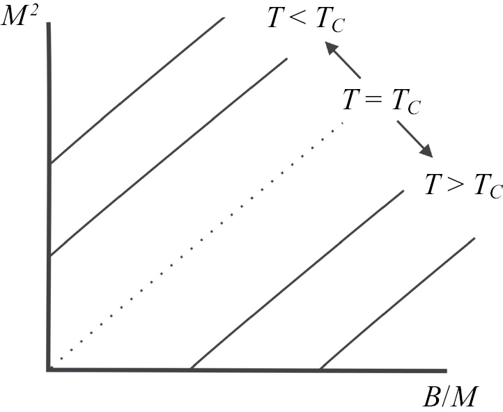
Figure 1.15 Schematic Arrott plots for an isotropic ferromagnet above and below the Curie temperature.

Hence, plotting M² versus B/M (Arrott plots shown in Figure 1.15) yields linear isotherms [59], the slopes of which do not change as a consequence of the assumption that b is temperature independent and the only coefficient changing with temperature is a. As one determines the intersection with either the x or the y-axis the lines are shifted parallel to one another as a function of temperature. The isotherm going through the origin defines the Curie temperature and the intercept on the M² axis (y-axis) enables the spontaneous magnetization in the ordered state to be determined. The intercept on the B/M axis provides the reciprocal of the susceptibility in the paramagnetic state. For T > T_C, $\chi =\frac{1}{2a}=\frac{1}{2a^{\prime }\left(T-T_C\right)}$, which is consistent with the molecular field theory and represents the Curie–Weiss law (Eq. (1.17)).

For an antiferromagnet, the transition occurs at the Néel temperature T_N and there are no anomalies at T_N in the Arrott plots. Instead of crossing the origin below the AF phase transition, the Arrott plots shift back in the opposite direction as compared to the case of the ferromagnet. An external magnetic field produces an additional shift in the AF phase transition, which has a quadratic dependence on the magnitude of the field, that is, ΔT_N is proportional to B².

It should be noted that the Landau theory on which this analysis is based is essentially a mean field description of the magnetic phase transition. Thus, magnetic fluctuations are neglected, even though close to the critical point of the phase transition they have large amplitudes and long lifetimes, and therefore cannot strictly be treated as small perturbations.

1.4.3 Critical Phenomena

As the transition at T_C is approached, the principal interest is the behavior of the thermodynamic properties that are assumed to have a simple power law dependence on the reduced temperature ε $=\frac{T-T_C}{T_C}$ and are characterized by a set of critical exponents [66]. A high degree of precision in the determination of both the order parameter and the temperature is required, and therefore the establishment of T_C is not straightforward. Furthermore, any comparison between measurements should be confined to results obtained within the same temperature interval Δε.

1.4.3.1 Thermal Dependence of the Order Parameter

In the limit of a small applied field, the spontaneous magnetization M_HT goes continuously to zero as T_C is approached. The thermal variation is given by [61]:

$M_{HT}=\underset{H_i\to 0}{\lim }M(H,T)\propto {\epsilon }^{\beta },$(1.66)

where the critical exponent β is observed to be < 1, typically taking values from 0.32 to 0.39 depending on the type of phase transition. We have introduced here the internal field H_i, given by [59]:

$H_i=H-N_{demag}M\left(H,T\right),$(1.67)

in which N_demag is the demagnetization factor and H the applied field.

1.4.3.2 Thermal Dependence of the Initial Susceptibility

As the temperature decreases toward T_C, the initial susceptibility diverges in a manner given by:

${\chi }_i={\left(\frac{\partial M}{\partial H_i}\right)}_{H_i\to 0}\propto {\epsilon }^{-\gamma },$(1.68)

where the critical exponent γ typically takes values from 1.3 to 1.4.

1.4.3.3 The Field Dependence of the Order Parameter along the Critical Isotherm

At the critical isotherm, T_C, the spontaneous magnetization is not a smooth function of the magnetic field but follows:

$M\left(H,T_c\right)\propto H_i{}^{\frac{1}{\delta }},$(1.69)

where the critical exponent δ typically takes values from 4.3 to 4.7. Reliable values of δ can only be obtained close to the critical point where ε is small, that is, if $\epsilon <{10}^{-2}$. According to Widom [62], the exponents β, γ, and δ should satisfy the relation γ = β (δ–1).

1.4.3.4 The Specific Heat

A singularity is observed in the specific heat at T_C in zero field, which can also be described by a power law:

$C\propto \{\begin{array}{c}{C}_{\uparrow }{\epsilon }^{-\alpha } T>T_C\\ -C_{\downarrow }{\epsilon }^{-{\alpha }^{\text{'}}} T<T_C\end{array}.$(1.70)

The constants $C_{\uparrow }$ and $C_{\downarrow }$ are observed to be different, whereas the exponents α and αʹ are found to be the same within the experimental error. Typical values of α and αʹ lie between 0.11 and 0.19.

1.4.3.5 The Thermal Variation of the Spin Density Fluctuations close to T_C

In order to describe neutron scattering, in 1954 van Hove [63, 64] introduced the concept of the pair distribution function $\tilde{G}$ between the atomic spin S₀ at lattice position zero, considered at time zero, and the atomic spin S_r, at lattice position r, considered at time t:

${\tilde{G}}_T\left(r,t\right)={〈S_0\left(0\right).S_r\left(t\right)〉}_T,$(1.71)

where <…>_T denotes the average over the thermal distribution. This pair distribution was included into the response (scattering) function $\tilde{S}(q,\omega )$ used to calculate the partial differential cross section for neutron scattering:

$\frac{{\text{d}}^2\sigma }{\text{d}\Omega \text{d}{E}_f}=N{r}_0^2\frac{k_f}{k_i}\tilde{S}(q,\omega ),$(1.72)

where q = k_i – k_f is the neutron wave vector change between initial to final state momenta, N is the number of unit cells in the sample, and r₀ = −5.4 fm = γ_n(e²/m_ec²) is the value of the neutron magnetic moment (γ_n = −1.913) multiplied by the classical electron radius, e²/m_ec² = 2.82 fm.

Van Hove [63] had already shown that due to large thermal fluctuations of the spin density as the temperature decreases toward T_C the neutron response function for magnetic scattering becomes:

$\tilde{S}\left(q,\omega \right)=\frac{1}{2\pi N\hslash }\underset{-\infty }{\overset{\infty }{\int }}{e}^{-i\omega t}{〈S^{\alpha }\left(-q,0\right)\cdot S^{\beta }(q,t)〉}_T\text{d}t,$(1.73)

where α and β are Cartesian coordinates x, y, and z.

In the static or quasi-static limit, assuming a localized model and neglecting the magnetic Bragg scattering contribution ~ ${〈S^{\alpha }〉}_T^2$, which is close to zero at T_C (paramagnetic scattering), the Fourier transform of the pair distribution function is given by:

$\tilde{\Gamma }\left(q\right)=\hslash \underset{0}{\overset{\infty }{\int }}\tilde{S}\left(q,\omega \right)\text{d}\omega =\frac{1}{2\pi N}\underset{-\infty }{\overset{\infty }{\int }}{e}^{-iqr}{〈\left(S\left(r\right)-〈S〉\right)\cdot \left(S\left(0\right)-〈S〉\right)〉}_T\text{d}V,$(1.74)

where the average spin density <S> is zero unless T<T_C or the applied field B ≠ 0. Thus (S(r) − <S>) represents fluctuations around the mean value of the magnetization. As T approaches T_C and q → 0, $\tilde{\Gamma }\left(q\right)$ diverges since both (S(r) − <S>) and (S(0) − <S>) remain correlated over large distances, with the range becoming infinite at T_C. Therefore, from Eq. (1.71), the static pair distribution or correlation function between a spin at position 0 and another at position r that is distance R away, in zero magnetic field is generally assumed to be isotropic, given by:

${\tilde{G}}_T\left(r\right)={〈S\left(0\right)\cdot S\left(r\right)〉}_T=\frac{f\left(\frac{R}{\xi }\right)}{R^{1+\eta }}.$(1.75)

The critical exponent η characterizes the behavior of the correlation function at T_C. Its magnitude is small and consequently, difficult to determine. For a classical model, η = 0. The correlation length ξ characterizes the spatial extent of the correlations and has a dependence on the reduced temperature ε given by ξ ∝ ε^–ν_. The magnitude of the critical exponent ν depends on the range of momentum transfer over which the measurements are made to determine ξ; typical values of ν are between 0.63 and 0.72. For T > T_C, the function $f\left(\frac{R}{\xi }\right)$ is assumed to have the form $f\left(\frac{R}{\xi }\right)=A{e}^{-\left(\frac{R}{\xi }\right)}$, where the constant A is only weakly dependent on ε.

As mentioned before, most magnetic transitions are second order, characterized by a continuous variation across the transition of the order parameter (the magnetization M_0T for ferromagnets and the staggered magnetization for ferrimagnets and antiferromagnets). This implies that the system is in a unique critical phase at the transition and long-range fluctuations cannot be neglected; Ginzburg showed this caused the general Landau mean-field theory of phase transitions to give incorrect predictions in the region near the transition. Work on the problem by researchers such as Widom [62], and Wilson and Kadanoff [65] on homogeneity, scaling laws, and renormalization gave rise to renormalization-group theory. This showed that continuous phase transitions all fall into one of a small number of classes with the same critical behavior, governed not by microscopic details of the system but its fundamental symmetries, such as the number of degrees of freedom n (of the spins for a magnetic system) and the number of spatial dimensions d.

A very important consequence is that all transitions in the same universality class should have the same critical exponents; for example, studying the superfluid phase transition in He⁴ (where the order parameter is the wavefunction describing the fraction of He atoms in the superfluid state, the amplitude and phase of which give two degrees of freedom) can provide useful information about the critical behavior of an planar ferromagnet or a superconductor, as all three systems are in the same universality class (where n = 2 and d = 3). Another consequence of the theory is that there must be relations between the critical exponents: any three critical exponents can be related by an inequality. Some of these inequalities are summarized below [66]:

$\begin{array}{c}\alpha +2\beta +\gamma =2;\\ 2-\alpha =\beta \left(\delta +1\right);\\ \gamma =\nu \left(2-\eta \right);\\ 2-\alpha =d\nu .\end{array}$(1.76)

In order to obtain actual predictions of the critical exponents, renormalization-group theory was applied to models consisting of discrete spins arranged in a regular lattice, which interact with the external field and their nearest neighbors only. The features of the most important models are briefly introduced below and their critical exponents are collected in Table 1.9.

2D Ising (n = 1, d = 2): The spins sit on the sites of a two-dimensional (2D) lattice (e.g. square and honeycomb) and are constrained to have only values s_i = ±1 pointing along a particular direction (e.g. up or down along the z-axis). The 2D Ising model is the only one on this list which has an exact solution.

2D XY (n = 2, d = 2): The spins are still confined to a single plane as for the 2D Ising model but can now point along any direction within that plane.

3D Ising (n = 1, d = 3): The spins now sit on the sites of a regular 3D lattice (e.g. simple cubic); they still interact with their nearest neighbors only and still take only values s_i = ±1 along one axis.

3D XY (n = 2, d = 3): The planes of 2D XY spins are stacked on top of each other; although the spins can only rotate in their own plane or layer, they can interact with the spins in the next adjacent layer.

Heisenberg (n = 3, d = 3): The spins can point in any direction in space and spin-spin interactions must therefore also be considered in three dimensions. This model is appropriate for isotropic ferromagnets.

It is worth noting that it is only possible to obtain the exact values of the critical exponents of the 2D Ising model in zero magnetic field. An exact solution in non-zero field for the behavior of the 2D Ising model or any of the 3D models are still open research questions; the critical exponents are therefore calculated numerically and are constantly being refined [67].

Table 1.9 Critical exponents of phase transitions calculated for various magnetic models and compared to measured values from real substances [66]–[68]. Values are exact for the mean-field theory and 2D Ising models.

Degrees of freedom	Exponents	$\beta$	$\delta$	$\eta$	$\alpha ={\alpha }^{\text{'}}$	$\gamma = {\gamma }^{\text{'}}$	$\nu = {\nu }^{\text{'}}$
		T < Tc	at T = Tc		${\alpha }^{\text{'}},{\gamma }^{\text{'}},{\nu }^{\text{'}}$ (T < Tc); $\alpha ,\gamma ,\nu$ (T > Tc)
	Models
	Mean-field	½	3	0	0	1	½
n = 1	2D Ising	⅛	15	¼	0	1¾	1
n = 1	3D Ising	0.3265	4.789	0.0364	0.110	1.2372	0.6301
n = 2	3D XY	0.34861	4.7801	0.03812	–0.01513	1.31782	0.67171
n = 3	Heisenberg (S = ½)	0.36893	4.7833	0.03755	0	1.39609	0.71125
	Measured
n = 1	Xe, Ar	0.341	–	0.0426	0.11	1.145	0.623
n = 2	4He, Gd2IFe2	0.347	–	-	–0.0127	1.320	0.6676
n = 3	Ni	0.395	4.35	-	–0.11	1.345	–

1.4.4 AC Susceptibility

The time-varying (dynamic) magnetization processes can be investigated using AC susceptibility measurements, where AC driving fields with frequencies ω between 10^–2–10⁵ s^–1 are superimposed on a DC background. If the magnetization M is subject to an alternating magnetic field $H=H_0{e}^{i\omega t}$, it is generally delayed by the phase angle δ$\left(\omega ,T\right)=\delta$ because of energy losses in the reversal process and is hence expressed as $M=M_0{e}^{i(\omega t-\delta )}$. The complex susceptibility $\chi \left(\omega ,T\right)=\frac{\partial M}{\partial H}$ can then be written as [11]:

$\chi \left(\omega ,T\right)=\frac{M_0}{H_0}{e}^{-i\delta }=\frac{M_0}{H_0}(\cos \delta -i\sin \delta )={\chi }^{\prime }\left(\omega ,T\right)-i{\chi }^{″}\left(\omega ,T\right),$(1.77)

where χʹ and χʺ are the in-phase (real) and out-of-phase (imaginary) susceptibility components, χʺ being proportional to the energy absorbed. For nanoparticles above the blocking temperature T_B, introduced in Section 1.3.3, χʺ is small and χʹ(ω,T) generally follows the Curie law ${\chi }^{\prime }\propto T^{-1}$, as expected for paramagnetic behavior. Assuming a single particle size from the slope of 1/χʹ versus T, the blocking temperature can be obtained and the particle volume can be estimated [69]. While the variation of χʹ is similar to that of χ_ZFC, χʺ peaks at T_B. However, the peak position and hence the measured value of T_B depend on the drive frequency (i.e. inverse measurement time) following Eq. (1.48). Comparison of the observed frequency dependence of T_B to the predictions given by the Néel–Brown equation (Eq. (1.42)) enables the presence of interparticle interactions, such as clustering due to dipole-dipole interaction to be identified. The presence of interparticle interactions gives rise to a stronger frequency dependence of the susceptibility [6, 70]. For non-interacting particles, both χʹ and χʺ are shifted to higher temperatures with increasing frequency. For interacting particles, the shift is more significant, as is the effect on the shape and height of the χʺ line shapes.

1.4.5 Mössbauer Spectroscopy

Mӧssbauer spectroscopy [71]–[74], which has a characteristic time scale τ_m ~ ns, has been used to investigate a number of systems using the isotope ⁵⁷Fe. Nuclei of this isotope emit gamma rays as they relax from their 3/2 excited state to the 1/2 ground state. By moving the ⁵⁷Fe source back and forth with a linear drive, the energy of the emitted gamma rays can be scanned via the Doppler effect to a very high degree of precision so as to enable recoilless (energy conservation) absorption by an Fe-containing sample. A typical range of velocities for a ⁵⁷Fe source is ±11 mm/s (1 mm/s = 48.075 neV) with a resolution down to ~1 neV. If the transmission spectrum versus source velocity is measured, a characteristic series of dips is observed. Below T_B, the relaxation time of the magnetization is long compared to τ_m and the spectrum is comprised of six lines due to the Zeeman splitting of the nuclear energy levels produced by the magnetic (hyperfine) field generated by the electrons. In a paramagnetic state this reduces to a single dip. By varying the sample temperature and measuring the area beneath the sextet of lines, T_B is estimated as the temperature at which the measured area beneath the sextet of lines is the same as the area beneath the superparamagnetic “central” dip.

The form of the time averaged magnetization $〈M\left(T\right)〉$ can be understood by realizing that the spins in a single domain nanoparticle act collectively as a macrospin, that is, they have a uniform precession angle. Therefore, it acts as a classical magnetic moment and the magnetization component along the quantization axis, $M_s\cos \theta$, can be calculated by Maxwell–Boltzmann statistical treatment and by using Eq. (1.32) [72]:

$〈M\left(T\right)〉=M_s\frac{{\int }_{-\pi /2}^{\pi /2}{e}^{\frac{-E\left(\theta \right)}{k_{B}T}}\cos \theta \sin \theta d\theta }{{\int }_{-\pi /2}^{\pi /2}{e}^{\frac{-E\left(\theta \right)}{k_{B}T}}\sin \theta d\theta }\approx M_s\left(1-\frac{k_{B}T}{2KV}\right).$(1.78)

For particles with uniaxial anisotropy, the magnetic hyperfine field B_hf is proportional to the average magnetization and is given by:

$〈B_{hf}〉=B_o\left(1-\frac{k_{B}T}{2KV}\right),$(1.79)

where B_o is the saturation hyperfine field, that is, the magnetic field acting on the nucleus in the absence of superparamagnetic relaxation. If a large field is applied above T_B and below T_C, the superparamagnetic relaxation is inhibited and the spectrum again comprises six lines. The average magnetic hyperfine splitting of the Mӧssbauer spectrum is then proportional to the high-field approximation $\left(\frac{\mu \left(T\right)B}{k_{B}T}>2\right)$ of the Langevin function (Eqs. (1.13) and (1.51)) [74]:

$〈B_{hf}〉=B_o\left(1-\frac{k_{B}T}{\mu \left(T\right)B}\right)-B,$(1.80)

where μ(T) = mμ_B = M(T)V is the magnetic moment of the particle, V is the particle volume, M(T) is the magnetization, and B is the applied field. A plot of $〈B_{hf}〉+B$ versus B^–1 yields a linear dependence, the gradient of which gives the moment, or if this is already established, the particle volume V = μ(T)/M_s.

1.4.6 Neutron Scattering

Neutron diffraction and XMCD can be used to determine the magnitude, direction, and anisotropy of atomic magnetic moments. Within the Born approximation, the differential cross section for elastic neutron scattering from the magnetic potential is given by [75]:

$\frac{\partial \sigma }{\partial \Omega }=r_0^2{\left|〈k_f,S^{\prime }|\frac{2}{\hslash }{\hat{S}}_n\cdot \int \left(e_q\times \left(\hat{M}\left(r\right)\times e_q\right)\right)e^{iq.r}d{r}^3|k_i,S〉\right|}^2,$(1.81)

where r₀ was introduced in Eq. (1.72), ${\hat{S}}_n$ is the spin-operator for the neutron, $e_q$ is the unit vector along q, and $\hat{M}\left(r\right)$ is the operator of the spatially dependent total magnetization, in which the neutron spin states S and Sʹ may change. The magnetic structure factor operator $\hat{Q}\left(q\right)=-\frac{1}{2{\mu }_B}\hat{M}\left(q\right)$ is related to $\hat{M}\left(q\right)$, the Fourier transform of $\hat{M}\left(r\right)$. Since $\hat{M}\left(q\right)$, also called the magnetic form factor, is a vector, each component may be complex:

$\hat{M}\left(q\right)={\int }^{\text{}}\hat{M}\left(r\right)e^{iq\cdot r}d{r}^3.$(1.82)

The scattering cross section is proportional to ${\left|〈S^{\prime }\left|\frac{2}{\hslash }{\hat{S}}_n\cdot {\hat{Q}}_{\perp }\left(q\right)\right|S〉\right|}^2$, where the magnetic interaction vector operator is ${\hat{Q}}_{\perp }\left(q\right)=e_q\times \left(\hat{Q}\left(q\right)\times e_q\right)$. A consequence of this relation is that neutrons only see the components of the magnetization perpendicular to the scattering vector. If the initial direction of the neutron spin is taken to be parallel to $e_z$, the direction of a magnetic field applied to the sample, then the cross section for scattering without change of the spin direction (non-spin-flip) is given by ${\left|e_z\cdot Q_{\perp }\left(q\right)\right|}^2={\left|Q_{\perp ,z}\left(q\right)\right|}^2$ and with a change of direction (spin-flip) by ${\left|e_z\times Q_{\perp }\left(q\right)\right|}^2$. The precise determination of the magnetization distribution in ferromagnetic materials makes use of the interference between the nuclear and magnetic scattering in which the sample is magnetized parallel to the spin direction of the incident polarized neutron beam. Assuming here that both the nuclear structure factor $N\left(q\right)=\sum _d{\overline{b}}_d{e}^{iq\cdot r}{e}^{-W_d}$ (where ${\overline{b}}_d$ is the average nuclear scattering length at atomic position d and W_d the Debye–Waller factor), and the magnetic structure factor Q(q) are real, the non-spin-flip scattering cross section is proportional to ${\left|N\left(q\right)\right|}^2\pm 2N\left(q\right)Q_{\perp ,z}\left(q\right)+{\left|Q_{\perp ,z}\left(q\right)\right|}^2$. The plus or minus sign refers to the neutron spin direction being parallel or anti parallel, respectively, to $Q_{\perp ,z}\left(q\right)$ and the quantity measured is the ratio of the two cross sections, namely the ‘polarization ratio’ $R=\frac{1+2\gamma + {\gamma }^2}{1-2\gamma + {\gamma }^2}$, where $\gamma = \frac{Q_{\perp ,z}\left(q\right)}{N\left(q\right)}$. This enables a precise determination of $Q_{\perp ,z}\left(q\right)$, which can then be compared directly with electronic structure calculations.

Neutron scattering with an intrinsic time scale of 10^–14–10^–7 s is particularly appropriate for studying the wavevector k and frequency ω of magnetic fluctuations [76]. Below T_B the magnetic response is not significantly affected by superparamagnetism, but relaxation and collective processes may occur. Relaxation processes are characterized by a quasi-elastic response centered on zero energy transfer (ω = 0), whereas collective excitations have a finite energy transfer [77]. For isotropic bulk ferromagnets, the long wavelength (k → 0) limit of the spin wave dispersion is ħω = Dk², as shown in Eq. (1.27). This defines a magnon wavelength given by:

$\lambda =2\pi \sqrt{\frac{D}{\hslash \omega }},$(1.83)

which for iron at 5 K corresponds to ~7 nm. Owing to the finite size of the particle, the collective excitation spectrum is quantized and therefore discrete. This may be demonstrated by considering the modes within a cuboid of side d. The spin wave energies are given by:

$E_n=D{k}_n^2=D{\left(\frac{n\pi }{d}\right)}^2,\text{with}n=1,2,3,\mathrm{...}$(1.84)

Thus, a spin wave gap Δ is produced given by:

$\Delta =D{\left(\frac{\pi }{d}\right)}^2,$(1.85)

which for 5 nm iron particles is about 11 meV. The presence of this gap significantly influences the thermodynamics of the particles. Hence, the low temperature thermal variation of the saturation magnetization is no longer given by the Bloch T^3/2 spin wave formula (Eq. (1.57)). On the basis of experimental results, a power law variation has been proposed:

$M\left(T\right)=M_s\left[1-B{T}^{\beta }\right],$(1.86)

where β depends on the particle size, varying between 2 down to 1.5 for bulk samples. On the basis of neutron scattering measurements, both quasi-elastic and inelastic features have been reported, the details of which are dependent on the system studied.

Through the fluctuation dissipation theorem [78], the imaginary part of the generalized susceptibility χ(q,ω) = χʹ(q, ω) + iχʺ(q, ω) is related to the response function for magnetic scattering $\tilde{S}\left(q,\omega \right)=\frac{1}{\pi }\frac{1}{\left(1-e^{-\frac{\hslash \omega }{k_{B}T}}\right)}{{\chi }^{″}}^{\left(q,\omega \right)}$. Hence, the frequency ω and wavevector dependence q of the response can be determined by neutron scattering. The uniform susceptibility (static q = 0 value) is often defined as per unit mass (χ_ρ) or per mole (χ_mol) and can be either positive or negative.

1.4.7 X-ray Magnetic Circular Dichroism (XMCD)

The XMCD technique is element specific while also allowing the spin and orbital contributions to the magnetic moment to be separated. In this process, a core electron in the examined material is excited to an empty valence state and the energy required is specific to the atomic species. In addition, due to the spin-orbit interaction, the X-ray absorption of a ferromagnet depends also on the relative orientation of the magnetization with respect to the direction of the incident photon spin. Since the transitions are governed by the Δ𝓁 = ±1 selection rule, d band transition metals are usually studied using the L_2,3 absorption edges (2p → 3d) [79, 80]. The spin and orbital moments are related to the absorption spectra σ⁺ and σ^– obtained with right-handed and left-handed circularly polarized X-rays by [81, 82]:

$m_L=〈L_Z〉\cdot {\mu }_B=2n_h\frac{{\int }_{L_3+L_2}{\sigma }^{+}-{\sigma }^{-}dE}{{\int }_{L_3+L_2}{\sigma }^{+}+{\sigma }^0+{\sigma }^{-}dE}\cdot {\mu }_B,$(1.87)

$m_S=2\left(〈S_Z〉+\frac{7}{2}〈T_Z〉\right)\cdot {\mu }_B=\frac{3}{2}{n}_h\frac{{\int }_{L_3}{\sigma }^{+}-{\sigma }^{-}dE-2{\int }_{L_2}{\sigma }^{+}-{\sigma }^{-}dE}{{\int }_{L_3+L_2}{\sigma }^{+}+{\sigma }^0+{\sigma }^{-}dE}\cdot {\mu }_B,$(1.88)

where <T_Z> is the expectation value of the dipole operator, n_h is the number of vacancies in the valence band (holes), σ⁰ = ½(σ⁺+σ^–) and the integral over the adsorption edges L₂ and L₃, and $\underset{L_3+L_2}{\int }dE$ is the sum of the areas under the absorption curves at the L₂ and L₃ energies. The number of holes, which can significantly differ from bulk for thin films or particles, can be determined by measuring the white line intensity by X-ray absorption spectroscopy. This involves taking an extra spectrum with linearly polarized X-rays in addition to the absorption spectra σ⁺ and σ^– required for XMCD.

1.5 Structural Analysis

Analysis of the microstructure is usually investigated using diffraction techniques, but real space imaging is also often employed. As a result of the X-ray adsorption in XMCD, secondary electrons are emitted, which can be analyzed by PEEM [83] to provide resolutions of up to ~10 nm. Transmission electron microscopy (TEM) provides information on the size and morphology of particles and the structure of thin films. If high resolution TEM is used, then atomic planes within samples can be imaged and possible imperfections, such as dislocations, identified. TEM has also been used to determine the size distribution of nanoparticles, which severely affects the magnetic properties and is a limiting factor in the interpretation of results. The volume distribution is generally found to follow a logarithmic-normal distribution of the form:

$f\left(V\right)=\frac{1}{\sigma \sqrt{2\pi }} exp\left[-\frac{{(\text{ln}\left(V\right)-\mu )}^2}{2{\sigma }^2}\right],$(1.89)

where σ is the standard deviation, σ² is the variance and μ is the mean of the variable’s natural logarithm. These are correlated to the mean, m, and variance, v, of the real sample values by:

$\mu =\text{ln}\left(\frac{m}{\sqrt{1+\frac{v}{m^2}}}\right),{\sigma }^2=\sqrt{\text{ln}\left(1+\frac{v}{m^2}\right)}.$(1.90)

When diffraction techniques are employed, X-rays [84] and neutrons [85] provide complementary measurements; in general, X-rays provide a better spatial resolution than neutrons. The broadening of diffraction peaks can arise from the domain size or microscopic strain. The broadening is usually characterized by the full width at half the maximum intensity (FWHM) of the Bragg peaks. The integral width, β_si (in radians), of a Bragg peak with index i at a scattering angle, 2θ_i, due to a small domain size is estimated by the Scherrer formula [86]:

${\beta }_{si}=\frac{K\lambda }{D_V\cos {\theta }_i},$(1.91)

where D_V is the volume-weighted domain size, λ is the wavelength of the incoming beam and K is a dimensionless shape factor with a value of about 0.9, which, however, varies with the actual shape of the crystallites. The integral width, β_di, due to microstrain can be approximated as [87]:

${\beta }_{di}=4ϵ\tan {\theta }_i,$(1.92)

where ε is the microstrain. Assuming a Cauchy-shaped profile (Lorentz distribution) for both the size and strain components, the corresponding integral widths are linearly additive:

${\beta }_{tot}={\beta }_{si}+{\beta }_{di} \underset{}{\iff }{\beta }_{tot}\cos {\theta }_i=\frac{K\lambda }{D_V}+4ϵsin{\theta }_i.$(1.93)

Thus, a plot (Williamson–Hall) [88] of ${\beta }_{tot}\cos {\theta }_i$ versus $\sin {\theta }_i$ for as many ${\theta }_i$ as possible should be linear, with the intercept giving $\frac{K\lambda }{D_V}$ and the gradient yielding 4ε.

An alternative method involves the convolution of the instrumental resolution D(θ) with a function (often a modified Voigt profile) representing the intrinsic line shape h(θ) to give the observed line shape I(θ), $I\left(\theta \right)=h\left(\theta \right)\otimes D\left(\theta \right)$. If the intrinsic and instrumental line shapes can both be represented by Gaussian functions, then the observed width ${\beta }_{obs}$ is given by:

${\beta }_{obs}={\left({\beta }_{intr}^2+{\beta }_{inst}^2\right)}^{\frac{1}{2}},$(1.94)

where ${\beta }_{intr} \text{and} {\beta }_{inst }$ are the intrinsic and instrumental integral widths. The instrumental resolution can be established using a standard sample.

Profile refinement programs, such as Fullprof [85], enable the full diffraction pattern to be analyzed, and possible anisotropic particle shapes and strains to be identified. Neutron diffraction also enables the possible magnetic structure of the particles to be established. If the particles are ferromagnetic, the magnetic scattering occurs at the nuclear positions. Heating above the Curie temperature will render the Bragg peaks entirely nuclear in origin, but this may change the nuclear structure. Alternatively, it may be possible to align the moments along the scattering vector to extinguish the magnetic Bragg component (Section 1.4.6). For some specific problems, the use of polarized neutrons may be required to uniquely extract the nuclear and magnetic contributions. However, if the particles have an AF structure, then, in general, the magnetic peaks occur at different Bragg positions. This distinction enables the nuclear and magnetic particle sizes to be established at the same temperature in the antiferromagnet NiO [89]. The spherical 6.5 nm particles have been found to have a 5.1 nm AF core with an outer shell of significantly reduced magnetization.

Sample Problems

Question 1

1. (a) Using Table 1.1, Eq. (1.5), and Hund’s rules, calculate S, L, J, p_J, and p_S for a Ti²⁺ ion (e.g. in a metallo-organic complex) and comment on how p_J and p_S compare to the experimental value.

2. (b) In similar fashion, calculate S, L, J, p_J, and p_S for a V²⁺ (or Mn⁴⁺) ion.

3. (c) In similar fashion, calculate S, L, J, p_J, and p_S for a Mn³⁺ (or Cr²⁺) ion.

Question 2

1. (a) By using Eq. (1.9), the expression for the mean square ionic radius $〈r^2〉=\frac{1}{Z}〈0\left|\sum _i{r}_i^2\right|0〉$, and the substitution $〈r^2〉=a_0^2$, calculate the value of the Larmor (molar) diamagnetic susceptibility for graphite (Z = 6) and compare it to the experimental value given in Table 1.4. Remember that the values in Table 1.4 are in CGS units, so the magnetic units conversion table in the Appendix should be used to convert from SI units.

2. (b) Repeat the exercise in (a) for Cu (Z = 29). Comment on the quality of the agreement.

3. (c) Repeat the exercise in (b) using instead the expression for the radius of the free electron sphere r_s given in Eq. (1.10) and the substitution $r_s^2=〈0\left|\sum _i{r}_i^2\right|0〉$, assuming a valence of 1 for Cu. Suggest a reason for the difference in the quality of the agreement between the newly calculated and experimental values.