Velocity and temperature scalings leading to compressible laws of the wall

Abstract

We exploit the similarity between the mean momentum equation and the mean energy equation and derive transformations for mean temperature profiles in compressible wall-bounded flows. In contrast to prior studies that rely on the strong Reynolds analogy and the presumed similarity between the instantaneous and mean velocity and temperature signals, the discussion in this paper involves the Farve-averaged equations only. We establish that the compressible momentum and energy equations can be made identical to their incompressible counterparts under appropriate normalizations and coordinate transformations. Two types of transformations are explored for illustration purposes: Van Driest (VD)-type transformations and semi-local-type or Trettel–Larsson (TL)-type transformations. In our derivations, it becomes clear that VD-type velocity and temperature transformations hold exclusively within the logarithmic layer. On the other hand, TL-type transformations extend their applicability to incorporate wall-damping effects, at least in principle. Each type of transformation serves its distinct purpose and has its applicable range. However, it is noteworthy that while VD-type transformations can be assessed using measurements obtained from laboratory experiments, TL-type transformations necessitate viscosity and density information typically accessible only through numerical simulations. Finally, we justify the omission of the turbulent kinetic energy transfer term, a term that is unclosed, in the energy equation. This omission leads to closed-form temperature transformations that are valid for both adiabatic and isothermal walls.

1. Introduction

The law of the wall asserts that the mean streamwise velocity $\langle u \rangle$ of an incompressible turbulent boundary layer is given by (von Kármán 1930; Prandtl 1932; Bradshaw & Huang 1995; Marusic et al. 2013)

(1.1)\begin{equation} \frac{\langle u \rangle }{u_\tau}=\frac{1}{\kappa} \log(y^+)+C,\end{equation}

in the ‘logarithmic’ region, i.e. $1\ll y^+$ and $y/\delta \ll 1$, where $\langle \rangle$ represents the conventional ensemble average (we reserve the symbol { } to indicate the Favre average), $\kappa$ and $C$ are constants, $y$ is the wall-normal coordinate and the superscript $+$ denotes normalization by wall units: $y^+ = \rho y u_\tau / \mu$, with $u_\tau =\sqrt {\tau _w/\rho }$ representing the friction velocity, $\tau _w$ the mean wall-shear stress and $\rho$ and $\mu$ respectively the fluid density and dynamic viscosity (both of which are constant in low-speed constant-property flows). Like other proposals for the turbulent boundary layer (Marusic & Monty 2019; Yang & Meneveau 2019), the law of the wall is empirical. Nonetheless, the log law in (1.1) has received considerable empirical and theoretical support (McKeon et al. 2004; Hultmark et al. 2012; Lee & Moser 2015; She, Chen & Hussain 2017; Xu & Yang 2018). Furthermore, the law of the wall is an anchor point for turbulence modelling – many models have been calibrated such that they reproduce the law of the wall for low-speed boundary-layer flows; well-known examples include wall functions for Reynolds-averaged Navier–Stokes (RANS) closures and the mixing-length models in large-eddy simulation wall models (Spalart & Allmaras 1992; Bose & Park 2018; Bin, Huang & Yang 2023).

Besides the mean velocity, the mean temperature above non-adiabatic walls in a low-speed boundary layer is also governed by the logarithmic scaling (Kays & Crawford 1980; Kader 1981; Bradshaw & Huang 1995). That is,

(1.2)\begin{equation} \frac{\langle T_w \rangle- \langle T \rangle}{T_\tau}=\frac{Pr_t}{ \kappa}\log(y^+)+C_T(Pr),\end{equation}

where $\langle T_w \rangle$ is the mean wall temperature, $T_\tau =\langle q_w \rangle /\rho _w c_pu_\tau$ is a temperature scale, $\langle q_w \rangle$ is the mean wall heat flux, $c_p$ is the specific heat, $Pr_t$ is the turbulent Prandtl number (assumed constant in the log layer) and $C_T = C_T(Pr)$ is the counterpart of $C$ in (1.1), which now depends on the molecular Prandtl number, $Pr$. Here, with the flow at a low speed, the momentum equation and the thermal equation are decoupled, and aerodynamic heating is negligible. Low-speed boundary layers satisfy the ‘Reynolds analogy’, in that the velocity and the temperature fields behave similarly (Pope 2000; Yang & Abkar 2018), which is why the mean temperature and the mean velocity are scaled in a similar form. As with the velocity scaling (1.1), the temperature scaling (1.2) has received much empirical support (Kim & Moin 1989; Abe, Kawamura & Matsuo 2004; Pirozzoli, Bernardini & Orlandi 2016), with the modelling of the turbulent Prandtl number at the centre of turbulence-modelling efforts (Kays 1994; Li 2019).

The incompressible form of the law of the wall in (1.1) becomes increasingly inaccurate with increasing Mach number, and the mean velocity in a compressible wall layer must be transformed before it can be described by the scaling in (1.1) (Morkovin 1962). Many velocity transformations have been proposed (Van Driest 1951; Zhang et al. 2012; Patel et al. 2015; Trettel & Larsson 2016; Griffin, Fu & Moin 2021). Like any model, these transformations have their applicable ranges. For instance, the Van Driest transformation works best for flows above adiabatic walls (Van Driest 1951), while the semi-local transformation works best for cold, isothermal walls (Trettel & Larsson 2016).

Regarding the mean temperature, the strong Reynolds analogy together with any velocity transformation gives the scaling of the mean temperature at high speeds. The strong Reynolds analogy was motivated by the similarity between the mean momentum equation and the mean energy equation when the molecular Prandtl number $Pr$ equals 1. The analogy assumes a similarity in the behaviour of velocity and temperature signals, linking velocity and temperature profiles within a compressible boundary layer. Here, we provide an overview of the development of the strong Reynolds analogy while examining its limitations in achieving a universal temperature scaling. Noteworthy contributors to the field include Busemann (1931), Crocco (1932), Morkovin (1962) and Walz (1959), whose collective efforts culminated in the formulation now recognized as Walz's equation. The equation establishes the mean temperature as a function of mean velocity, free-stream temperature and recovery temperature. This early proposal was extended by Cebeci (1974), Gaviglio (1987), Huang, Coleman & Bradshaw (1995), Duan & Martin (2011) and Zhang et al. (2014) to accommodate diabatic walls, non-unit molecular Prandtl numbers and large fluctuations in total temperatures, among other deviations from the assumptions upon which the strong Reynolds analogy is based. These extensions, however, rely heavily on empirical functions. For instance, the work by Duan & Martin (2011) invoked empirical functions that express the recovery temperature as a function of the velocity. Excessive dependence on empiricism poses limitations. From a practical standpoint, empirical functions are usually valid only at the calibration conditions. From a model development perspective, the constant need for new corrections implies that the strong Reynolds analogy is a poor approximation of real turbulence. This concern gains credence through discussions of its inadequacies in prior studies (e.g. Guarini et al. 2000; Maeder, Adams & Kleiser 2001; Liang & Li 2013; Wenzel, Gibis & Kloker 2022). In particular, as the Mach number increases, the mean momentum equation and the mean energy equation become increasingly dissimilar due to aerodynamic heating (Yang et al. 2018; Wenzel et al. 2022), at least for air.

The strong Reynolds analogy is not absolutely necessary for establishing a temperature scaling. We can approach the temperature scaling like we have approached the velocity scaling, and derive explicit $y$ scalings for the mean temperature, or temperature transformations. Following this line of thought, we first examine the explicit $y$ scaling in (1.2). This scaling is not sufficient. In fact, for adiabatic walls, $T_\tau =0$ and $\langle T_w \rangle -\langle T\rangle \neq 0$, and the left-hand side of (1.2) is undefined. This leaves us with temperature transformations. Transformations for the temperature have received less attention than those for the velocity. The bulk of the work on the topic has been to calibrate the turbulent Prandtl number (Kays 1994; Weigand, Ferguson & Crawford 1997; Li 2019; Lusher & Coleman 2022). These studies concern themselves with the turbulent heat flux term in the energy equation, which is unclosed in the RANS equations. The only work on temperature transformation seems to be that by Patel, Boersma & Pecnik (2017) and Chen et al. (2022). In Patel et al. (2017) a temperature transformation was obtained by assuming similarity between the mean temperature and the mean velocity. The temperature transformation, however, is singular for adiabatic walls. Chen et al. (2022) attempted a unified description for mean temperature above both isothermal and adiabatic walls, but their transformations depend heavily on direct numerical simulation (DNS) inputs and are not closed.

The objective of this work is to exploit the similarity between the mean momentum and energy equations in both the incompressible and compressible regimes so that we can extend the law of the wall for both mean velocity and mean temperature from the incompressible regime to the compressible regime. For the mean temperature, we follow a strategy similar to the one in Chen et al. (2022), but our transformations are closed and predictive. We also test the resulting temperature transformations against isothermal- and adiabatic-wall data from recent DNS of supersonic plane-channel flows (Lusher & Coleman 2022).

The rest of the paper is organized as follows. In § 2, we review the law of the wall for the mean velocity and temperature for incompressible conditions. We parametrize the eddy viscosity and the turbulent Prandtl number to provide references for the discussion that follows. In § 3, we simplify and non-dimensionalize the mean momentum and mean energy equations in the compressible regime. We show that turbulent kinetic energy transport terms are negligible compared with mean kinetic energy transport terms. The equations look quite different from their incompressible counterparts. In §§ 4 and 5, we utilize the equations we obtained in § 3 and follow the velocity transformations of Van Driest and Trettel & Larsson, respectively, to derive temperature transformations. We show that the compressible momentum and energy equations can be made identical under appropriate normalizations and transformations. Finally, concluding remarks are provided in § 6.

2. Incompressible law of the wall

In this section, we review the incompressible law of the wall and formulate the turbulent Prandtl number based on the recently obtained DNS data. The results here provide baselines for subsequent sections.

We consider the inner layer of the turbulent boundary layer where constant values of the total shear stress and heat flux can be assumed. Integrating the governing equations for velocity and temperature in the inner region of the boundary layer gives

(2.1)\begin{equation} \langle \tau_{12} \rangle-\langle \rho u'v' \rangle =\langle \tau_w \rangle \end{equation}

and

(2.2)\begin{equation} -\langle q_{y} \rangle- c_p \langle \rho v'T' \rangle= - \langle q_w \rangle,\end{equation}

where $\tau _{12}$ is the molecular shear stress. By assuming constant molecular viscosity, $\mu$, heat capacity, $c_p$, and Prandtl number, $Pr$, the Newtonian fluxes become

(2.3)\begin{equation} \langle \tau_{12} \rangle= \mu \frac{ {\rm d} \langle u \rangle}{{\rm d} y} \end{equation}

and

(2.4)\begin{equation} -\langle q_{y} \rangle= \frac{\mu}{Pr} c_p \frac{ {\rm d} \langle T \rangle }{{\rm d} y}. \end{equation}

Moreover, by applying the Boussinesq/eddy-viscosity assumptions for turbulent shear stress and heat flux, $-\langle \rho u'v' \rangle =\mu _t \,{\rm d} \langle u \rangle /{\rm d} y$ and $-c_p \langle \rho v'T' \rangle =(\mu _t/ {Pr}_t) c_p \,{\rm d} \langle T \rangle /{\rm d} y$, we can write (2.1) and (2.2) as follows:

(2.5)\begin{equation} ( \mu+\mu_t ) \frac{{\rm d} \langle u \rangle}{{\rm d} y}=\langle \tau_w \rangle \end{equation}

and

(2.6)\begin{equation} \left( \frac{\mu}{Pr}+\frac{\mu_t}{{Pr}_t}\right) c_p \frac{{\rm d} \langle T \rangle}{{\rm d} y}= - \langle q_w \rangle, \end{equation}

where ${Pr}_t$ is the turbulent Prandtl number to be defined in (2.14). Equations (2.5) and (2.6) can be further written in dimensionless form using the two wall-scaling quantities $u_\tau = (\langle \tau _w \rangle /\rho )^{1/2}$ and $T_\tau =\langle q_w \rangle /(\rho c_p u_\tau )$:

(2.7)\begin{equation} \left( 1 + \frac{\mu_t}{\mu} \right) \frac{{\rm d} u^+}{{\rm d} y^+}=1 \end{equation}

and

(2.8)\begin{equation} \left(\frac{1}{Pr}+ \frac{\mu_t/\mu}{{Pr}_t} \right) \frac{{\rm d} T^+}{{\rm d} y^+}=1,\end{equation}

where $u^+=\langle u \rangle /u_\tau$ and $T^+=( \langle T_w \rangle - \langle T \rangle )/T_\tau$ are the dimensionless velocity and temperature, and $y^+=\rho u_\tau y/\mu$ is the dimensionless wall distance. Equation (2.8) can also be rewritten in terms of another dimensionless temperature, $\theta = (\langle T_w \rangle -\langle T \rangle )/\langle T_w \rangle$, and the dimensionless temperature equation becomes

(2.9)\begin{equation} \left(\frac{1}{Pr}+ \frac{\mu_t/\mu}{{Pr}_t} \right) \frac{{\rm d} \theta}{{\rm d} y^+}=B_q,\end{equation}

where $B_q=-\langle q_w \rangle /\rho u_\tau c_p \langle T_w \rangle$. Equations (2.8) and (2.9) have their advantages and disadvantages. Equation (2.8) is valid for isothermal walls only. For adiabatic walls, the dimensionless temperature $T^+$ cannot be defined because $T_\tau$ is zero. Nonetheless, under isothermal wall conditions, a unique law of the wall can be identified for $T^+$ (Kays & Crawford 1980; Kader 1981; Bradshaw & Huang 1995), which is a benefit. Equation (2.9) is valid for both adiabatic and isothermal walls, which is an advantage, but the solution of $\theta$ depends on $B_q$, which, compared with the velocity scaling in (1.1) that does not explicitly depend on the wall flux, is a slight disadvantage.

The profiles for the turbulent viscosity and the velocity are approximated by

(2.10)\begin{equation} \frac{\mu_t}{\mu} = \kappa y^+ \end{equation}

and

(2.11)\begin{equation} u^+ = \frac{1}{\kappa} \ln y^+ + C\end{equation}

in the log layer, where $\kappa$ is the von Kármán constant and $C$ is the intercept; a good fit to the data gives rise to $\kappa \approx 0.41$ and $C\approx 5.2$, respectively, although the exact values may vary slightly depending on the flow configuration (Marusic et al. 2013). There are many proposals that describe how the turbulent viscosity or/and velocity profiles transition from the no-slip condition to the log layer. The most popular one was presented by Van Driest using an exponential damping function to the turbulent mixing length (Van Driest 1956). However, the Van Driest damping fails to satisfy asymptotic near-wall behaviour, yielding $\mu _t \propto y^4$ instead of the correct asymptotic behaviour of $\mu _t \propto y^3$. Johnson & King (1985) proposed a damping function that satisfies the near-wall asymptotic behaviour:

(2.12)\begin{equation} \frac{\mu_t}{\mu} = \kappa y^+ D,\end{equation}

where $D = [1-\exp (-y^+/A^+)]^2$ and $A^+=17$. Furthermore, by assuming a constant turbulent Prandtl number in the log layer, the temperature equation yields

(2.13)\begin{equation} T^+ = \frac{{Pr}_t}{\kappa} \ln y^+ + C_T,\end{equation}

with ${Pr}_t=0.85$ and $C_T=3.9$ (Kays & Crawford 1980).

Here, we used DNS data from two incompressible passive scalar channel flows to examine the law of the wall for temperature. We refer to the two datasets as AA (Abe & Antonia 2019) and LHP (Lluesma-Rodriguez, Hoyas & Perez-Quiles 2018). A comparison of the turbulent Prandtl number is shown in figure 1. Here, the turbulent Prandtl number is defined as

(2.14)\begin{equation} {Pr}_t=\frac{ \langle u'v' \rangle }{\langle v'T' \rangle} \frac {{\rm d} \langle T \rangle /{\rm d} y}{{\rm d} \langle u \rangle /{\rm d} y}. \end{equation}

As $y \rightarrow 0$, both $\langle u'v' \rangle$ and $\langle v'T' \rangle$ decrease as $y^3$ while both temperature and velocity gradients approach constant values. Due to $0/0$-limiting behaviour near the wall, ${Pr}_t$ becomes very sensitive to numerical errors as it approaches the wall (Chen et al. 2023). Moreover, the DNS results indicate $Pr_t$ depends somewhat on Reynolds numbers, as shown in figure 1(a). Alternatively, one may define a total Prandtl number as

(2.15)\begin{equation} {Pr}_{total}{=\frac{\text{total viscosity}}{\text{total conductivity}}}=\frac{\mu+\mu_t}{\mu/Pr+\mu_t/Pr_t}=\frac{1+\mu_t/\mu} {1/Pr+(\mu_t/\mu)/Pr_t}. \end{equation}

The result is shown in figure 1(b). We observe the following. Firstly, the total Prandtl number collapses to a universal profile for a given molecular Prandtl number in the region where $y^+<10$, while for large values of $y^+$, $Pr_{total}$ returns to $Pr_t$. Secondly, the total (or turbulent) Prandtl number peaks at $y^+ \approx 50$. Thirdly, the profiles in this region depend on the Reynolds number: for large Reynolds numbers, $Re_\tau >1000$, one may assume a constant total (or turbulent) Prandtl number of 0.85 beyond $y^+>150$. Lastly, we note that the difference between two DNS solutions with almost the same Reynolds number ($Re_\tau \approx 1000$) is as large as that caused by the Reynolds number effects. Hence, the DNS-computed turbulent Prandtl numbers are affected by numerical and/or statistical errors.

Figure 1. (a) Turbulent Prandtl number. (b) Total Prandtl number. Dataset AA is from Abe & Antonia (2019) and LHP is from Lluesma-Rodriguez et al. (2018) and the $Pr_{total}$ model correlation is from (2.12), (2.15) and (2.16).

The following expression provides a good working approximation for ${Pr}_t$:

(2.16)\begin{equation} {Pr}_t=1.05-0.2 \tanh^3 \left( \frac{y^+}{A^+_{Pr}} \right)\!.\end{equation}

It follows that a similar thermal conductivity damping for temperature can be defined, and due to (2.12), we have

(2.17)\begin{equation} \frac {\mu_t/\mu}{{Pr}_t}= \frac{\kappa}{{Pr}_t} y^+ D,\end{equation}

where $A^+_{Pr} = 70$ yields a good fit to the DNS data. Equation (2.16) assumes a value of 1.05 in the viscous sublayer and drops to 0.85 between the buffer and the log layers ($30< y^+<300$). It also ensures $\langle v'T' \rangle$ decreases as $y^3$ towards the wall, which is a desirable physical feature. The modelled turbulent and total Prandtl numbers are shown by the thick black lines in figures 1(a) and 1(b). The non-monotonic behaviour of the turbulent Prandtl number in the buffer layer region is ignored in the model, as it is likely due to the uncertainties in the DNS result as mentioned above. We use (2.16) as a reference below, when DNS data of compressible flows are analysed.

Before we proceed to the compressible regime, we show DNS for the turbulent thermal conductivity and dimensionless temperature profiles in figure 2. The solution obtained with the model equations, i.e. (2.17) and (2.8), is also presented for comparison. The agreement in the inner layer is very good, and it appears that for large values of $Re_\tau$, a law of the wall closely resembling the empirical logarithmic temperature equation proposed in Kays & Crawford (1980), (2.13), emerges.

Figure 2. (a) Turbulent conductivity. (b) Temperature profiles. Dataset AA refers to Abe & Antonia (2019) and LHP refers to Lluesma-Rodriguez et al. (2018). The model correlation in (a) is from (2.17) and the temperature correlation is from the solution of (2.8) using (2.17).

3. The energy equation in high-speed flows

In this section, we simplify the mean momentum and energy equations, non-dimensionalize them and discuss the universality of the turbulent Prandtl number and the turbulent eddy viscosity.

We utilize the data in Lusher & Coleman (2022). The data are DNS of compressible turbulence between two no-slip plane walls and mixed thermal boundary conditions, specifically, with one adiabatic wall and one isothermal wall. The flow configuration is shown in figure 3. The data cover a significant range of Reynolds numbers with mean/core Mach numbers between 1.2 and 2.2. Although the two sides of the channel flows are not independent, the first- and second-order statistics of the flow are largely defined by the boundary conditions of the nearest wall, as shown by Lusher & Coleman (2022). Hence, each of the two sides can reasonably be expected to emulate the physics of an isolated isothermal or adiabatic wall layer. The details of Lusher & Coleman's DNSs are summarized in table 1 for data near the isothermal-wall side and table 2 for data near the adiabatic-wall side, where the case prefix (‘i’ or ‘a’) indicates the thermal boundary condition. For example, ‘iB’ and ‘aB’ refer to respectively the isothermal-wall and adiabatic-wall sides. Notice that the Reynolds number range covered by the adiabatic-wall cases is lower than that covered by the isothermal cases. The lower Reynolds numbers of the adiabatic-wall cases are due to the higher temperature, and thus the higher molecular viscosity, near the adiabatic wall. The reader is referred to Lusher & Coleman (2022) for further information regarding the numerical strategy, its validation and the fidelity of the results.

Figure 3. Schematic of the DNS by Lusher & Coleman (2022). The DNS studies both isothermal and adiabatic wall conditions in a channel. The coordinate $y_e$ is where the maximum velocity is located, and $y_0$ is the location where the molecular viscosity experiences a step change; see Lusher & Coleman (2022) for further details about the step change in the molecular viscosity. In the present study, whichever of $y_e$ and $y_0$ is closer to the adiabatic or isothermal wall defines the effective thickness of the boundary layer adjacent to that particular wall.

Table 1. Details of cold/isothermal-wall-side cases, where ${Re}_{\tau _{iw}}=\rho _{iw} u_{\tau,iw} h/\mu _{iw}$, $M_{\tau _{iw}}=u_{\tau,iw}/c_{\tau,iw}$, $B_q=\langle q_{iw} \rangle /(\rho _{iw} u_{\tau,iw} c_p T_{iw}$) and $\langle T_e \rangle$ is the temperature at the free stream, as defined by figure 3.

Table 2. Details of hot/adiabatic-wall-side cases, where ${Re}_{\tau _{aw}}=\langle \rho _{aw} \rangle u_{\tau,aw} h/\langle \mu _{aw} \rangle$, $M_{\tau _{aw}}=u_{\tau,aw}/\langle c_{\tau,aw} \rangle$ and $\langle T_e \rangle$ is the temperature at the free stream, as defined by figure 3.

First, we simplify the mean momentum and energy equations in the high-speed regime. Invoking the constant-stress and constant-total-energy-flux idealizations as in Pope (2000), we have

(3.1)\begin{equation} \langle \tau_{12} \rangle -\langle \rho u'' v'' \rangle = \langle \tau_w \rangle \end{equation}

and

(3.2)\begin{equation} - \langle q_y \rangle- c_p \langle \rho v'' T'' \rangle +\langle u_i \rangle \langle \tau_{i2} \rangle - \langle \rho v''K'' \rangle+\langle u'_i \tau'_{i2} \rangle-\langle \rho v''k'' \rangle = - \langle q_w \rangle. \end{equation}

The two equations describe the mean momentum and energy balances. The first and second terms on the left-hand side in (3.1) are the molecular and turbulent shear stresses, respectively. They are

(3.3)\begin{equation} \langle \tau_{12} \rangle=\left\langle \mu \frac{{\partial} u}{{\partial} y} \right\rangle \approx \langle \mu \rangle \frac{{\rm d} \{ u \}}{{\rm d} y} \end{equation}

and

(3.4)\begin{equation} -\langle \rho u'' v'' \rangle \approx \mu_t \frac{{\rm d} \{ u \}}{{\rm d} y}. \end{equation}

In (3.3), terms involving $\langle u'' \rangle$ and $\langle \mu ' {\partial } u'/{\partial } y \rangle$ are neglected since they are small compared with their counterparts that involve $\{ u \}$ and $\langle \tau _{12} \rangle$ (Huang et al. 1995). Here, Boussinesq's viscosity hypothesis is invoked. The left-hand side of (3.2) represents the fluxes of the total energy, $e + u_i^2/2$. Here, $e$ is the internal energy and $u_i^2/2$ is the kinetic energy and is often ignored in incompressible flow. We define the decomposition of the kinetic energy following Huang et al. (1995):

(3.5)\begin{equation} \frac{u_i u_i}{2}=\{K\}+K''+\{k\}+k'', \end{equation}

where $\{K\} = \{u_i\}\{u_i\}/2$, $K''=\{u_i\}u''_i$, $\{k\} = \{u''_i u''_i\}/2$ and $k''=u''_i u''_i/2 -\{ k \}$. This decomposition gives rise to the last four terms on the left-hand side of (3.2). The first, third and fifth terms are the molecular diffusive fluxes of the mean temperature, $\{T\}$, and mean and turbulent kinetic energies, $\{K\}$ and $\{k\}$, respectively, which are

(3.6)$$\begin{gather} - \langle q_y \rangle \approx \frac{ \langle \mu \rangle}{Pr} c_p \frac{{\rm d} \{ T \}}{{\rm d} y}, \end{gather}$$

(3.7)$$\begin{gather}\langle u_i \rangle \langle \tau_{i2} \rangle \approx \{ u \} \langle \mu \rangle \frac{{\rm d} \{ u \}}{{\rm d} y} \end{gather}$$

and

(3.8)\begin{equation} \langle u'_i \tau'_{i2} \rangle \approx \langle \mu \rangle \frac{{\rm d} \{ k \}}{{\rm d} y}. \end{equation}

The second, fourth and sixth terms in (3.2) are the turbulent fluxes of $\{T\}$, $\{K\}$ and $\{k\}$, respectively, for which Boussinesq's hypothesis yields

(3.9)$$\begin{gather} - c_p \langle \rho v'' T'' \rangle \approx \frac{ \mu_t }{{Pr}_t} c_p \frac{{\rm d} \{ T \}}{{\rm d} y}, \end{gather}$$

(3.10)$$\begin{gather}- \langle \rho v''K'' \rangle= - \{u\} \langle \rho u''v''\rangle \approx \{u\} \mu_t \frac{{\rm d} \{ u \}}{{\rm d} y}, \end{gather}$$

(3.11)$$\begin{gather}- \langle \rho v''k'' \rangle= - \langle \rho v'' u''_i u''_i \rangle/2 \approx \frac{ \mu_t }{Pr_k} \frac{{\rm d} \{ k \}}{{\rm d} y}, \end{gather}$$

where $Pr_t$ and $Pr_k$ are the turbulent Prandtl numbers for temperature, $\{T\}$, and turbulent kinetic energy, $\{k\}$. Note that (3.10) implies the Prandtl number of the turbulent diffusive flux of the mean kinetic energy $\{K\}$ is unity. (Compare the right-hand sides of (3.7) and (3.10).) The sum of fluxes of mean kinetic energy, i.e. the sum of (3.7) and (3.10), can be evaluated explicitly with the help of the momentum equation, (3.1):

(3.12)\begin{equation} \{ u \} \langle \mu \rangle \frac{{\rm d} \{ u \}}{{\rm d} y}- \{u\} \langle \rho u''v''\rangle=\{ u\} \langle \tau_w \rangle. \end{equation}

A reasonable simplification is that the fluxes of the mean kinetic energy are much larger than those of turbulent kinetic energy. That is, the terms in (3.7) and (3.10) are larger than the terms in (3.8) and (3.11). It follows that (3.1) and (3.2) can be written as

(3.13)\begin{equation} ( \langle \mu \rangle+\mu_t ) \frac{{\rm d} \{ u \} }{{\rm d} y}=\langle \tau_w \rangle \end{equation}

and

(3.14)\begin{equation} \left( \frac{\langle \mu \rangle}{Pr}+\frac{\mu_t}{Pr_t}\right) c_p \frac{{\rm d} \{ T \}}{{\rm d} y}= - \langle q_w \rangle-\{ u\} \langle \tau_w \rangle, \end{equation}

where

(3.15)\begin{equation} {Pr}_t=\frac{ \langle \rho u''v'' \rangle }{\langle \rho v''T'' \rangle} \frac {{\rm d} \{T\} /{\rm d} y}{{\rm d} \{ u \} /{\rm d} y}. \end{equation}

We can verify the above assumption with data. Figure 4 shows the fluxes for cases iF2 (table 1) and aF2 (table 2). Similar conclusions were observed for the other cases. We see that the molecular and turbulent fluxes of the mean kinetic energy, i.e. $\langle u_i \rangle \langle \tau _{i2} \rangle$ and $- \langle \rho v''K'' \rangle$, are much larger than the molecular and turbulent fluxes of the turbulent kinetic energy, $\langle u'_i \tau '_{i2} \rangle$ and $-\langle \rho v''k'' \rangle$ in the wall layer. We note that this is not a trivial observation: although the mean kinetic energy is much larger than the turbulent kinetic energy, it is not immediately clear that the transport of the mean kinetic energy is much larger than the transport of the turbulent kinetic energy. In fact, the transport of the turbulent part of a flow quantity is often larger than the transport of its mean part in a boundary layer. For instance, the transfer of the turbulent part of the momentum is larger than the transport of the mean momentum. Furthermore, we can also see from figure 4 that there is a close agreement between the sum of the molecular and turbulent diffusive fluxes of the mean kinetic energy and $\{u\} \langle \tau _w \rangle$ close to the wall.

Figure 4. Energy fluxes, (3.2), for cases iF2 and aF2. The quantities are scaled by $\rho _b V_\tau ^3$, where $\rho _b=\int _{-h}^{+h}\langle \rho \rangle \,{\rm d} y/2h$ and $V_\tau ^2=(\tau _{iw}+\tau _{aw})/2 \rho _b$; see Lusher & Coleman (2022).

Next, we non-dimensionalize the mean momentum and energy equations. Non-dimensionalization of the flow quantities at high speeds is not as straightforward as it is at low speeds. Two types of non-dimensionalization are often used, namely wall scaling and semi-local scaling. The wall scaling involves the mean values at the wall: $\langle \rho _w \rangle$, $\langle \mu _w \rangle$, $\{T_w\}$, $\langle \tau _w \rangle$ and $\langle q_w \rangle$. For example, the wall friction velocity is $u_\tau =(\langle \tau _w \rangle /\langle \rho _w \rangle )^{1/2}$. Following the practice in the low-speed regime, we define $T_\tau =\langle q_w \rangle /(\langle \rho _w \rangle u_\tau c_p)$ and non-dimensionalize the energy equation. With $u_\tau$ and $T_\tau$, (3.13) and (3.14) can be written in dimensionless form as

(3.16)\begin{equation} \left( \frac{\langle \mu \rangle}{\langle \mu_w \rangle} + \frac{\mu_t}{\langle \mu_w \rangle} \right) \frac{{\rm d} u^+}{{\rm d} y^+}=1 \end{equation}

and

(3.17)\begin{equation} \left(\frac{ \langle \mu \rangle/\langle \mu_w \rangle}{Pr}+ \frac{\mu_t/\langle \mu_w \rangle}{{Pr}_t} \right) \frac{{\rm d} T^+}{{\rm d} y^+}=\frac{B_q+(\gamma-1) M_\tau^2 u^+}{B_q},\end{equation}

where $u^+ = \{u\}/u_\tau$, $T^+=(\{T_w\}-\{T\})/T_\tau$, $B_q= \langle q_w \rangle /( \langle \rho _w \rangle u_\tau c_p \langle T_w \rangle )$ and $M_\tau =u_\tau /(\gamma R \langle T_w \rangle )^{1/2}$. Like the incompressible equation for $T^+$, i.e. (2.8), (3.17) here poses difficulty in adiabatic cases. Introducing $\theta = ({T_w}-{T})/{T_w}$, (3.14) can be recast as

(3.18)\begin{equation} \left(\frac{ \langle \mu \rangle/\langle \mu_w \rangle}{Pr}+ \frac{\mu_t/\langle \mu_w \rangle}{{Pr}_t} \right) \frac{{\rm d} \theta}{{\rm d} y^+}=B_q+(\gamma-1) M_\tau^2 u^+.\end{equation}

Equation (3.18) is a more general form of the dimensionless temperature equation, as it applies to both adiabatic and isothermal cases. However, unlike the incompressible $\theta$ equation, (2.9), whose right-hand side is zero when the wall is adiabatic, the right-hand side of (3.18) does not equal zero when the wall is adiabatic, due to viscous heating. Comparing (3.16) and (3.18), we see that the strong Reynolds analogy breaks down due to the second term on the right-hand side of (3.18). It may be interesting to see if the law of the wall can be preserved through some temperature transformation for both isothermal and adiabatic wall conditions. Before doing so, the similarity of the dimensionless viscosity and turbulent Prandtl number between the incompressible and compressible flows must be investigated.

This calls for the semi-local scaling (Huang et al. 1995). The dimensionless locally scaled turbulent viscosity, $\mu _t/\langle \mu \rangle$, and the total Prandtl number are plotted against a wall distance defined by the local mean properties, $y^* = \langle \rho \rangle (\langle \tau _w \rangle / \langle \rho \rangle )^{1/2} y/\langle \mu \rangle$, in figures 5 and 6 for isothermal- and adiabatic-wall data, respectively. For comparison, the incompressible formula for $Pr_{total}$, (2.15), is also depicted in these figures, in which all the properties are normalized according to the semi-local scaling:

(3.19)$$\begin{gather} \frac{\mu_t}{\langle \mu \rangle} = \kappa y^* D^*, \end{gather}$$

(3.20)$$\begin{gather}\frac{\mu_t}{\langle \mu_w \rangle} =\left( \frac{\langle \rho \rangle }{\langle \rho_w \rangle }\right)^{1/2} \kappa y^+ D^* \end{gather}$$

and

(3.21)\begin{equation} {Pr}_t=1.05-0.2 \tanh^3 \left( \frac{y^*}{A^*_{Pr}} \right)\!, \end{equation}

where $D^* = [1-\exp (-y^*/A^*)]^2$ and $A^*$ takes the same value as the incompressible one, 17 (Yang & Lv 2018); $A^*_{Pr}$ is also assumed to have the same incompressible-flow value, 70. Equations (3.19) and (3.21) are shown by the thick black lines in figures 5 and 6. As can be seen from the figures, both $\mu _t/\langle \mu \rangle$ and ${Pr}_{total}$ scale very well with $y^*$, which is in agreement with the observation by Huang et al. (1995) in their early work. Compared with the data at incompressible conditions, the values of $\mu _t/\langle \mu \rangle$ have a slightly wider spread in the buffer-layer region, and the profiles are slightly below the law-of-the-wall line. Furthermore, the total Prandtl number seems to fall somewhat below (3.21). Although a better match could be adjusted by choosing a smaller value of $A^*_{Pr}$, we did not attempt to do so since a unified description at both low and high Mach numbers is preferred.

Figure 5. Plots of (a) $\mu _t/\mu$ and (b) total Prandtl number scaling with $y^*$ for isothermal-wall DNS data.

Figure 6. Plots of (a) $\mu _t/\mu$ and (b) total Prandtl number scaling with $y^*$ for adiabatic-wall DNS data.

4. Van Driest-type transformations

In this section, we explore Van Driest-type transformations and their effectiveness in collapsing temperature data. Within the log-layer region, the molecular components of the diffusion terms can be safely neglected, leading to the simplification of (3.16) and (3.18) as follows:

(4.1)\begin{equation} \frac{\mu_t}{\langle \mu_w \rangle} \frac{{\rm d} u^+}{{\rm d} y^+}=1 \end{equation}

and

(4.2)\begin{equation} \frac{\mu_t/\langle \mu_w \rangle}{{Pr}_t} \frac{{\rm d} \theta}{{\rm d} y^+}=B_q +(\gamma-1) M_\tau^2 u^+. \end{equation}

By substituting (3.20) and $D^*=1$ into (4.1) and (4.2), one gets

(4.3)\begin{equation} \left( \frac{\langle \rho \rangle }{\langle \rho_w \rangle }\right)^{1/2} \frac{{\rm d} u^+}{{\rm d} y^+}=\frac{1}{\kappa y^+} \end{equation}

and

(4.4)\begin{equation} \frac{1}{B_q +(\gamma-1) M_\tau^2 u^+} \left( \frac{\langle \rho \rangle }{\langle \rho_w \rangle } \right)^{1/2} \frac{{\rm d} \theta}{{\rm d} y^+}=\frac{{Pr}_t}{\kappa y^+}. \end{equation}

Inspired by (4.3), Van Driest introduced the following transformation for mean velocity, aimed at extending the law of the wall to compressible boundary layers (Van Driest 1951):

(4.5)\begin{equation} u_{VD}^+ = \int_0^{u^+} \left( \frac{\langle \rho \rangle }{\langle \rho_w \rangle }\right)^{1/2} \,{\rm d} u^+. \end{equation}

Here, we follow the same spirit and define a similar transformation for the temperature:

(4.6)\begin{equation} T_{VD}^+ = \int_0^{\theta} \frac{1}{B_q +(\gamma-1) M_\tau^2 u^+} \left( \frac{\langle \rho \rangle }{\langle \rho_w \rangle } \right)^{1/2} \,{\rm d} \theta. \end{equation}

These transformations are expected to result in velocity and temperature profiles that share the same slopes as their incompressible counterparts within the logarithmic region:

(4.7)\begin{equation} \frac{{\rm d} u_{VD}^+}{{\rm d} y^+}=\frac{1}{\kappa y^+} \end{equation}

and

(4.8)\begin{equation} \frac{{\rm d} T_{VD}^+}{{\rm d} y^+}=\frac{{Pr}_t}{\kappa y^+}. \end{equation}

There are at least two ways to assess the transformations in (4.5) and (4.6). The first approach involves closed-form solutions using experimentally measurable quantities, as proposed by Van Driest (referred to as VD1) (Van Driest 1951). The second approach (referred to as VD2) evaluates the transformation using the density ratio profile obtained from DNS. We derive VD1 in the following. Firstly, the ideal gas law gives

(4.9)\begin{equation} \frac{\langle \rho \rangle }{\langle \rho_w \rangle }=\frac{\langle T_w \rangle }{\langle T \rangle }. \end{equation}

Secondly, by dividing (4.4) by (4.3), we have

(4.10)\begin{equation} \frac{1}{B_q +(\gamma-1) M_\tau^2 u^+} \frac{{\rm d} \theta}{{\rm d} u^+}={Pr}_t. \end{equation}

The integration of (4.10) can be performed with the assumption that ${Pr}_t$ is a constant:

(4.11)\begin{equation} \frac{\langle T \rangle }{\langle T_w \rangle }=1-{Pr}_t B_q u^+ - {Pr}_t (\gamma -1) M_\tau^2 \frac{{u^+}^2}{2}, \end{equation}

where a value of 0.9 for ${Pr}_t$ was used in Huang & Coleman (1994). The more recent work by Lusher & Coleman (2022) and the data in Kays (1994), however, suggest ${Pr}_t=0.85$. Note that the Van Driest transformation, as originally derived by Van Driest, is restricted to the log region. This restriction arises due to the absence of damping terms in (4.3) and (4.4). Consequently, (4.11) is derived exclusively for the log region, where ${Pr}_t$ is indeed approximately constant. Finally, by substituting (4.9) and (4.11) into (4.5) and (4.6), we obtain the VD1 transformation for velocity (Van Driest 1951; Rotta 1960; Huang & Coleman 1994):

(4.12)\begin{equation} u_{VD}^+ = \int_0^{u^+} \frac{1}{( 1-{Pr}_t B_q u^+ - {Pr}_t (\gamma -1) M_\tau^2 {u^+}^2/2 )^{1/2}} \,{\rm d} u^+ ,\end{equation}

and temperature:

(4.13)\begin{equation} T_{VD}^+ = \int_0^{\theta} \frac{1}{B_q +(\gamma-1) M_\tau^2 u^+} \frac{1}{( 1-{Pr}_t B_q u^+ - {Pr}_t (\gamma -1) M_\tau^2 {u^+}^2/2 )^{1/2}} \,{\rm d} \theta. \end{equation}

Equations (4.12) and (4.13) depend on $B_q$ and $M_\tau$, $\langle T_w \rangle$, $\langle \tau _w \rangle$ and $\langle q_w \rangle$, all of which are defined at the wall. Van Driest (1951) and Rotta (1960) obtained an analytic form of the transformed velocity, $u_{VD}^+$, but in the analysis here, numerical transformation is applied to both (4.12) and (4.13) due to the lack of an analytic solution for (4.13).

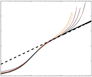
The transformed velocity and temperature of the DNS solutions are illustrated in figures 7 and 8, respectively. For the isothermal-wall cases, there is a wide spread of the transformed velocity and temperature profiles near the sub- and buffer layers. This spread can be explained by investigating the molecular portion of the diffusion terms in (3.16) and (3.17). Close to the wall, we have

(4.14)\begin{equation} \frac{{\rm d} u_{VD}^+}{{\rm d} y^+}= \frac{\langle \mu_w \rangle}{\langle \mu \rangle}\left( \frac{\langle \rho \rangle}{\langle \rho_w \rangle} \right)^{1/2}=\left( \frac{\langle T_w \rangle}{\langle T \rangle} \right)^{1.2} \end{equation}

and

(4.15)\begin{equation} \frac{{\rm d} T_{VD}^+}{{\rm d} y^+}=Pr \frac{\langle \mu_w \rangle}{\langle \mu \rangle}\left( \frac{\langle \rho \rangle}{\langle \rho_w \rangle} \right)^{1/2}=Pr \left( \frac{\langle T_w \rangle}{\langle T \rangle} \right)^{1.2}, \end{equation}

where $\langle \mu \rangle /\langle \mu _w \rangle \approx (\langle T \rangle /\langle T_w \rangle )^{0.7}$ is invoked. We see that the two derivatives depend on the temperature. Different temperature distributions therefore lead to different values of $u_{VD}^+$ and $T_{VD}^+$ at the onset of the log layer. This has a particularly strong effect on isothermal walls. In contrast, the transformed velocity and temperature profiles near the adiabatic wall show less spread, because $T_w/\langle T\rangle$ is approximately a constant near the wall. Despite a mismatch of the transformed profiles near the sub- and buffer layers, figures 7 and 8 show that VD1 gives the right slopes, $\kappa \approx 0.41$ and $\kappa _T \approx 0.41/0.85$ in the log-layer region.

Figure 7. Van Driest's velocity transformation in (4.5) of DNS data. The legends in (a,b) are the same as in figures 5(a) and 6(a).

Figure 8. Van Driest's temperature transformation in (4.6) of DNS data. The legends in (a,b) are the same as in figures 5(a) and 6(a).

The VD2 solution is compared with the VD1 solution in figure 9. For the adiabatic cases, the differences between VD1 and VD2 are almost negligible, and therefore we show only case iE. For comparison purposes, the un-transformed velocity and temperature profiles are included. We see that both VD1 and VD2 give rise to the same incompressible velocity and temperature slope in the log-layer region, with VD1 matching the law-of-the-wall reference slightly better. Furthermore, we see that changing the value of the turbulent Prandtl number in the logarithmic region from 0.85 to 0.9 does not significantly affect the result. This is likely because terms other than ${v''T''}$ are also significant. It should be noted that the other cases also show the same trend and are not shown here for brevity.

Figure 9. Comparison of VD1, i.e. the transformation in (4.5) and (4.6), and VD2, i.e. the transformation in (4.12) and (4.13), for case iE.

5. Semi-local-type transformations

Trettel & Larsson (2016), along with others like Pecnik & Patel (2017), employed the semi-local scaled wall-normal coordinate. The resulting transformations are, in principle, valid in the viscous layer. The definitions of $y^+$ and $y^*$ yield the following expressions:

(5.1)\begin{equation} y^*=\frac{\langle \mu_w \rangle}{\langle \mu \rangle} \left( \frac{\langle \rho \rangle}{\langle \rho_w \rangle} \right)^{1/2} y^+ \end{equation}

and

(5.2)\begin{equation} \frac{\partial y^*}{\partial y^+}=\frac{\langle \mu_w \rangle}{\langle \mu \rangle} \left( \frac{\langle \rho \rangle}{\langle \rho_w \rangle} \right)^{1/2} \left[ 1+ \frac{1}{2}\frac{y^+}{\langle \rho \rangle} \frac{\partial \langle \rho \rangle}{\partial y^+}-\frac{y^+}{\langle \mu \rangle} \frac{\partial \langle \mu \rangle}{\partial y^+} \right]\!. \end{equation}

Substituting these two expressions into (3.16) and (3.17), one obtains the following equations:

(5.3)\begin{equation} \left( 1 + \frac{\mu_t}{\langle \mu \rangle} \right) \left( \frac{\langle \rho \rangle}{\langle \rho_w \rangle} \right)^{1/2} \left[ 1+ \frac{1}{2}\frac{y^+}{\langle \rho \rangle} \frac{\partial \langle \rho \rangle}{\partial y^+}-\frac{y^+}{\langle \mu \rangle} \frac{\partial \langle \mu \rangle}{\partial y^+} \right] \frac{{\rm d} u^+}{{\rm d} y^*}=1 \end{equation}

and

(5.4)\begin{equation} \left(\!\frac{1}{Pr}+ \frac{\mu_t/\langle \mu \rangle}{{Pr}_t}\!\right) \frac{1}{B_q +(\gamma-1) M_\tau^2 u^+} \left(\!\frac{\langle \rho\rangle}{\langle \rho_w \rangle} \!\right)^{1/2} \left[ 1+ \frac{1}{2}\frac{y^+}{\langle \rho \rangle} \frac{\partial \langle \rho \rangle}{\partial y^+}-\frac{y^+}{\langle \mu \rangle} \frac{\partial \langle \mu \rangle}{\partial y^+} \right] \frac{{\rm d} \theta}{{\rm d} y^*}=1. \end{equation}

Trettel & Larsson (2016) defined the following transformation for velocity:

(5.5)\begin{equation} u_{TL}^+ = \int_0^{u^+} \left( \frac{\langle \rho \rangle}{\langle \rho_w \rangle} \right)^{1/2} \left[ 1+ \frac{1}{2}\frac{y^+}{\langle \rho \rangle} \frac{\partial \langle \rho \rangle}{\partial y^+}-\frac{y^+}{\langle \mu \rangle} \frac{\partial \langle \mu \rangle}{\partial y^+} \right] {\rm d} u^+. \end{equation}

Here, we follow the same spirit and define a Trettel & Larsson (TL)-type transformation for temperature:

(5.6)\begin{equation} T_{TL}^+ = \int_0^{\theta} \frac{1}{B_q +(\gamma-1) M_\tau^2 u^+} \left( \frac{\langle \rho \rangle}{\langle \rho_w \rangle} \right)^{1/2} \left[ 1+ \frac{1}{2}\frac{y^+}{\langle \rho \rangle} \frac{\partial \langle \rho \rangle}{\partial y^+}-\frac{y^+}{\langle \mu \rangle} \frac{\partial \langle \mu \rangle}{\partial y^+} \right] {\rm d} \theta. \end{equation}

These two transformations lead to the following velocity and temperature equations:

(5.7)\begin{equation} \left( 1 + \frac{\mu_t}{\langle \mu \rangle} \right) \frac{{\rm d} u_{TL}^+}{{\rm d} y^*}=1\end{equation}

and

(5.8)\begin{equation} \left(\frac{1}{Pr}+ \frac{\mu_t/\langle \mu \rangle}{{Pr}_t} \right) \frac{{\rm d} T_{TL}^+}{{\rm d} y^*}=1. \end{equation}

When evaluated at the wall, the two equations do not explicitly depend on the temperature. Consequently, both $u^+_{TL}$ and $T^+_{TL}$ are uniquely defined when $Pr$ is given. Furthermore, since (5.7) and (5.8) share the same structure as their incompressible counterparts, and considering that $\mu _t/\langle \mu \rangle$ and $Pr_t$ scale similarly with $y^*$ as their counterparts scale with $y^+$ in incompressible flows, one would expect the transformed velocity and temperature to exhibit behaviour akin to incompressible flows. This is an advantage compared to the VD transformations. However, unlike VD1, TL transformation requires local density and molecular viscosity information, or at least temperature information to link to density and molecular viscosity profiles – and these profiles must be sufficiently accurate to provide adequate evaluations of density and viscosity gradients. Thus TL transformations require access to local, internal mean profiles from, for example, numerical simulations. This is a major practical disadvantage of TL-type transformations.

In figures 10 and 11, the transformed velocity and temperature are evaluated numerically using density and molecular viscosity profiles along with their derivatives extracted directly from the DNS data. Additionally, the figures include numerical solutions of (5.7) and (5.8) using the eddy viscosity and turbulent Prandtl number closures specified in (3.19) and (3.21). These reference solutions mirror the incompressible inner layer but with $y^+$ replaced by $y^*$. As depicted in the figures, the isothermal cases exhibit close agreement between the incompressible law of the wall and the transformed velocity and temperature within the inner layer. In contrast, for the adiabatic cases, while the slopes of the transformed velocity and temperature profiles match the incompressible law of the wall, the intercept constants of the transformed velocity and temperature ($C$ and $C_T$) exceed their corresponding incompressible values. This is likely a low-Reynolds-number effect, as observed in figure 6: the high temperatures near the adiabatic surfaces lead to large molecular viscosities and enhanced viscous effects, which, in turn, cause a delayed transition from the viscous layer to the log layer, contributing to larger log-layer intercepts.

Figure 10. Results of the TL velocity transformation. The legends in (a,b) are the same as in figures 5(a) and 6(a).

Figure 11. Results of the TL-type temperature transformation. The legends in (a,b) are the same as in figures 5(a) and 6(a).

Lastly, we comment on the validity of the TL-type temperature transformation in (5.6) for spatially developing boundary-layer configurations. The TL velocity transformation in (5.5) is known to underperform in boundary layers. Whether the TL temperature transformation would also underperform in boundary layers is not immediately clear, since the behaviour of a velocity transformation is not perfectly correlated with the behaviour of its temperature counterpart. Here we evaluate (5.6) for one boundary-layer dataset from Zhang et al. (2014) to illustrate our point. The flow is at a friction Reynolds number of 550 and a Mach number of 2.00. The wall is adiabatic. Figure 12 shows the result. The TL-transformed velocity deviates further from the incompressible law of the wall compared with the VD-transformed velocity – this is expected. Conversely, the TL- and VD-transformed temperature profiles are not very different. A more detailed assessment of the performance of the temperature transformations in channel, boundary-layer and other configurations is outside the scope of the present work and is left for future investigation.

Figure 12. Results of the TL and VD transformations for a boundary-layer flow in Zhang et al. (2014).

6. Conclusions

We examine the mean temperature equations in the incompressible and compressible conditions, specifically, (2.8), (2.9), (3.17) and (3.18), and explore the similarity between the temperature and velocity equations at low and high speeds. We argue that one need not rely on the Reynolds analogy for scaling estimates of the temperature in compressible flows. Rather, one can obtain temperature scalings in the same manner as velocity scalings/transformations. The purpose of velocity and temperature transformations is to convert the compressible equations to their incompressible counterparts. The VD-type transformations accomplish this conversion in the logarithmic layer (see (4.7) and (4.8)). Therefore, VD-type transformations are valid only in the logarithmic layer, with the transformed velocity and temperature profiles having the same log-law slope as their incompressible counterparts, but different intercepts. The TL-type transformations, in principle, hold in both the viscous layer and the logarithmic layer (see (5.7) and (5.8)). A posteriori tests, however, reveal that TL-type temperature transformations leave room for improvement above adiabatic walls, with the intercepts of the transformed temperature profiles significantly larger than their incompressible counterpart – although the degree to which this is caused by the low Reynolds numbers induced by high temperatures near the adiabatic wall is an open question. Overall, each type of transformation serves its distinct purpose and has its applicable range. It is nonetheless worth noting that VD-type transformations can be assessed using wall measurements, whereas TL-type transformations necessitate viscosity and density information typically accessible only through numerical simulations.

The current approach sets itself apart from prior studies that rely on the strong Reynolds analogy. Instead of presuming similarity between velocity and temperature signals, the current approach capitalizes on the universality of eddy viscosity and turbulent Prandtl number with respect to the transformed wall-normal coordinate and the similarity between the energy and the momentum equations. Furthermore, by neglecting the turbulent-kinetic-energy transport term in the energy equation (after verifying its insignificance) and accounting for viscous heating, our approach leads to closed-form temperature transformations that are valid for both isothermal and adiabatic walls. The attainment of closed forms and unified descriptions for isothermal and adiabatic walls is critical to turbulence modelling, and applications of the transformations in (4.5), (4.6), (4.12), (4.13), (5.5) and (5.6) in the context of RANS and large-eddy simulations are to be of significant value. That said, while the present approach allows us to borrow insights gained from previous work on velocity and velocity transformations, and not needing the presumed similarity between the velocity and temperature signals is a strength of the present approach, a drawback is the lack of scaling estimates for temperature fluctuations. The mean velocity scaling and the scaling of velocity fluctuations were independently established by von Kármán and Townsend, with the latter introducing the concept of attached eddies. Similarly, new concepts are needed here in order to establish scalings or transformations for temperature fluctuations, a topic recommended for future study.