Inertial migration of a sphere in plane Couette flow

Abstract

We study the inertial migration of a torque-free neutrally buoyant sphere in wall-bounded plane Couette flow over a wide range of channel Reynolds numbers $Re_c$ in the limit of small particle Reynolds number ($Re_p\ll 1$) and confinement ratio ($\lambda \ll 1$). Here, $Re_c = V_{wall}H/\nu$, where $H$ denotes the separation between the channel walls, $V_\text {wall}$ denotes the speed of the moving wall, and $\nu$ is the kinematic viscosity of the Newtonian suspending fluid. Also, $\lambda = a/H$, where $a$ is the sphere radius, with $Re_p=\lambda ^2 Re_c$. The channel centreline is found to be the only (stable) equilibrium below a critical $Re_c$ ($\approx 148$), consistent with the predictions of earlier small-$Re_c$ analyses. A supercritical pitchfork bifurcation at the critical $Re_c$ creates a pair of stable off-centre equilibria, located symmetrically with respect to the centreline, with the original centreline equilibrium becoming unstable simultaneously. The new equilibria migrate wall-ward with increasing $Re_c$. In contrast to the inference based on recent computations, the aforementioned bifurcation occurs for arbitrarily small $Re_p$ provided that $\lambda$ is sufficiently small. An analogous bifurcation occurs in the two-dimensional scenario, that is, for a circular cylinder suspended freely in plane Couette flow, with the critical $Re_c$ being approximately $110$.

1. Introduction

Some of the first observations of cross-stream migration of neutrally buoyant spherical particles, in an ambient shearing flow, were the experiments of Segre & Silberberg (1962a,b) involving pipe flow of a dilute suspension of such particles. For small values of the pipe Reynolds number, the spheres were found to accumulate at an intermediate annulus, about $0.6$ times the pipe radius from the centreline, creating a ‘tubular pinch’ effect. Cross-stream migration of spheres in a unidirectional shearing flow is prohibited by the time-reversibility of the Stokes equations, and the observed migration is due to inertial lift forces, occurring only for non-zero particle Reynolds numbers. As described in more detail in Anand & Subramanian (2023b), a number of theoretical and numerical studies have since attempted to explain these observations, the first one being that of Ho & Leal (1974), albeit for a shearing flow in a two-dimensional channel geometry. Ho & Leal (1974) determined the inertial lift force on a sphere for both the plane Couette and plane Poiseuille velocity profiles, within a point-particle framework, for $Re_c\ll 1$, where $Re_c$ is the channel Reynolds number. While the lift force in plane Poiseuille flow also equalled zero at a location intermediate between the wall and the centreline, consistent with the observed intermediate equilibrium in the Segre–Silberberg experiments, that in plane Couette flow always pointed towards the channel centreline, rendering this location the only stable equilibrium. A subsequent more accurate calculation of the lift force profiles, again for $Re_c \ll 1$, was performed by Vasseur & Cox (1976) using a Green's function formulation developed earlier by Cox & Brenner (1968).

Later, Feng, Hu & Joseph (1994) carried out finite element computations for a neutrally buoyant circular cylinder in plane Couette flow for $\lambda =0.125$ with $Re_p=0.625$ and $1.25$. Here, $\lambda$ is the confinement ratio, defined as the ratio of the cylinder radius to the inter-wall spacing, with $Re_p = \lambda ^2\,Re_c$ being the particle Reynolds number; the point-particle limit corresponds to $\lambda \ll 1$, and $Re_c=40$ and $80$ in the effort of Feng et al. (1994), with the authors still obtaining the channel centreline as the only stable equilibrium, consistent with the predictions of the aforementioned small-$Re_c$ analyses. Very recently, the motion of both a neutrally buoyant circular cylinder (Fox, Schneider & Khair 2020) and sphere (Fox, Schneider & Khair 2021), again in plane Couette flow, was studied using lattice-Boltzmann simulations. The parameter ranges corresponding to $0.1\leq Re_p\leq 50$ and $0.1\leq \lambda \leq 0.2$ ($0.1\leq Re_p\leq 50$ and $0.0625\leq \lambda \leq 0.25$) were examined for the sphere (cylinder), with the associated maximum $Re_c$ significantly exceeding that in Feng et al. (1994). The larger-$Re_c$ simulations led to the authors finding the emergence of stable off-centre equilibria via a pitchfork bifurcation. For a given $\lambda$, the sphere migrated to the only (stable) equilibrium at the centreline below a critical $Re_p$, while above this critical value, a pitchfork bifurcation led to an unstable equilibrium at the centre, with a pair of symmetrically located stable equilibria on either side of the centreline. While the simulations pointed to a decrease in the critical $Re_p$ with decreasing $\lambda$, owing to the limited range of parameters examined, it remained unclear as to whether the bifurcation was a signature of a finite $Re_p$ (as implied, for instance, in the abstracts of the said articles), or if it correlated to a threshold level of inertia on scales of order the channel width. Herein, we show that the latter is the case. That is, the bifurcation threshold in plane Couette flow, for both a circular cylinder and a sphere, is shown to correspond to a critical $Re_c$ rather than $Re_p$, and this is accomplished via a point-particle formulation similar to that used by Schonberg & Hinch (1989) to study inertial migration in plane Poiseuille flow at finite $Re_c$.

The paper is organized as follows. Section 2 discusses the governing equations and boundary conditions for a neutrally buoyant sphere suspended freely in plane Couette flow, for arbitrary $Re_c$, in the limit $Re_p \ll 1$ (implying $\lambda \ll 1$). In § 3, the inertial lift velocity is determined semi-analytically for $Re_c \ll 1$ using a reciprocal theorem formulation. Inertia acts as a regular perturbation in this limit, the lift velocity being $O(Re_p)$ and its calculation requiring only knowledge of the velocity fields induced by a Stokeslet and a stresslet confined between (infinite) parallel plane boundaries. In § 4, the lift velocity is calculated for $Re_c\gtrsim O(1)$, with inertia now acting as a singular perturbation. Similar to Schonberg & Hinch (1989), this calculation involves obtaining coupled second-order ordinary differential equations (ODEs) for the partially Fourier transformed pressure and normal velocity fields, and then solving the associated boundary value problem numerically using a shooting method. The results for the equilibrium loci, in § 5, reveal a supercritical pitchfork bifurcation at $Re_c\approx 148$; the analogous calculation for a circular cylinder shows a bifurcation at $Re_c \approx 110$. We conclude in § 6 by discussing the effects of finite particle size on the bifurcation surface in $s_{eq}$–$Re_c$–$\lambda$ space – where $s_{eq}$ denotes the (transverse) equilibrium position of the sphere within the channel – and commenting briefly on the role of non-neutral buoyancy.

2. Formulation

Figure 1 shows a schematic of a neutrally buoyant sphere suspended in a Newtonian fluid undergoing plane Couette flow between infinite boundaries separated by a distance $H$. Using the sphere radius $a$ and the velocity scale $\dot {\gamma }a$, $\dot {\gamma }=V_{wall}/H$ being the ambient shear rate, the equations governing the fluid motion, in non-dimensional form, are given by

(2.1a)$$\begin{gather} \nabla^2 \boldsymbol{u}-\boldsymbol{\nabla}p =Re_p\,\boldsymbol{u}\boldsymbol{\cdot}\boldsymbol{\nabla}\boldsymbol{u}, \end{gather}$$

(2.1b)$$\begin{gather}\boldsymbol{\nabla}\boldsymbol{\cdot}\boldsymbol{u}=0 , \end{gather}$$

where $Re_p=a^2\dot {\gamma }/\nu$ is the particle Reynolds number, and $\nu$ is the kinematic viscosity of the suspending fluid. The unsteady acceleration term has been neglected in (2.1a), and the necessary justification for this is provided at the end of § 4.

For $\lambda \ll 1$, at leading order, the neutrally buoyant sphere translates with the velocity of the plane Couette flow at its centre, while rotating with half the ambient vorticity. In a reference frame centred at the sphere, and translating with this velocity, $\boldsymbol {u}$ still satisfies (2.1a) and (2.1b) with the following boundary conditions:

(2.2a)$$\begin{gather} \boldsymbol{u}={-}\tfrac{1}{2}\boldsymbol{1}_3\wedge \boldsymbol{r} \quad \text{for } \boldsymbol{r}\in S_p, \end{gather}$$

(2.2b)$$\begin{gather}\boldsymbol{u}\rightarrow r_2\boldsymbol{1}_1 \quad \text{for } r_1,r_3\rightarrow \infty\ (r_2\ \text{fixed}), \end{gather}$$

(2.2c)$$\begin{gather}\boldsymbol{u}={-}\lambda^{{-}1}s\boldsymbol{1}_1\quad \text{at}\ r_2={-}s\lambda^{{-}1}\ \text{(lower wall)}, \end{gather}$$

(2.2d)$$\begin{gather}\boldsymbol{u}={-}\lambda^{{-}1}(1-s)\boldsymbol{1}_1 \quad \text{at}\ r_2=(1-s)\lambda^{{-}1}\ \text{(upper wall)}. \end{gather}$$

Here, $S_p$ denotes the surface of the sphere, and $s=d/H$ denotes its (non-dimensional) transverse location within the channel; see figure 1. In terms of the corresponding disturbance fields, $\boldsymbol {u}'=\boldsymbol {u}-\boldsymbol {u}^\infty$, $p'=p-p^\infty$ ($\boldsymbol {u}^\infty = r_2\boldsymbol {1}_1$, $p^\infty$ being an arbitrary constant), the governing equations may be written as

(2.3a)$$\begin{gather} \nabla^2 \boldsymbol{u}'-\boldsymbol{\nabla} p' =Re_p\,(\boldsymbol{u}'\boldsymbol{\cdot}\boldsymbol{\nabla}\boldsymbol{u}'+\boldsymbol{u}'\boldsymbol{\cdot} \boldsymbol{\nabla}\boldsymbol{u}^\infty+\boldsymbol{u}^\infty\boldsymbol{\cdot}\boldsymbol{\nabla}\boldsymbol{u}'), \end{gather}$$

(2.3b)$$\begin{gather}\boldsymbol{\nabla}\boldsymbol{\cdot} \boldsymbol{u}'=0, \end{gather}$$

with boundary conditions (2.2a–d) taking the form

(2.4a)$$\begin{gather} \boldsymbol{u}'={-}\tfrac{1}{2}\boldsymbol{1}_3\wedge \boldsymbol{r}- r_2\boldsymbol{1}_1 \quad \text{for } \boldsymbol{r}\in S_p, \end{gather}$$

(2.4b)$$\begin{gather}\boldsymbol{u}'\rightarrow 0 \quad \text{for } r_1,r_3\rightarrow \infty\ (r_2\ \text{fixed}), \end{gather}$$

(2.4c)$$\begin{gather}\boldsymbol{u}'=0\quad \text{at}\ r_2={-}s\lambda^{{-}1}, (1-s)\lambda^{{-}1}. \end{gather}$$

Figure 1. Schematic of a neutrally buoyant sphere suspended in wall-bounded plane Couette flow.

It is well known that one requires a matched asymptotics expansions approach to solve the Navier–Stokes equations for small but finite $Re_p$ (Proudman & Pearson 1957). The matching of an inner expansion, valid in the neighbourhood of the particle, and an outer expansion, valid at distances of order the so-called inertial screening length, is in general necessary to calculate inertial corrections. For an ambient linear shearing flow, the screening length is $a\,Re_p^{-1/2}$ (Saffman 1965), or alternatively $H\,Re_c^{-1/2}$. The latter expression shows that the walls lie in the inner Stokesian region for $Re_c\ll 1$, with fluid inertia being a regular perturbation (see § 3). When $Re_c\gtrsim O(1)$, the inertial screening length is of order the channel width or smaller, and the walls lie in the so-called Oseen region. Fluid inertial effects now constitute a singular perturbation, and one must solve the linearized Navier–Stokes equations, with the solution being a function of $Re_c$ at leading order (see § 4).

3. The inertial lift velocity for $Re_c\ll 1$

In this section, we revisit the inertial lift calculation for $Re_c \ll 1$, a problem first addressed by Ho & Leal (1974) and Vasseur & Cox (1976). A generalized reciprocal theorem formulation yields the following expression for the inertial lift velocity (Anand & Subramanian 2023b):

(3.1)\begin{equation} V_p={-}Re_p\int\boldsymbol{u}^{(2)}\boldsymbol{\cdot}(\boldsymbol{u}^{(1)'}\boldsymbol{\cdot}\boldsymbol{\nabla}\boldsymbol{u}^{(1)'}+ \boldsymbol{u}^{(1)'}\boldsymbol{\cdot}\boldsymbol{\nabla} \boldsymbol{u}^\infty+\boldsymbol{u}^\infty \boldsymbol{\cdot}\boldsymbol{\nabla}\boldsymbol{u}^{(1)'})\,{\rm d} V. \end{equation}

In (3.1), problem (1) denotes the one described in § 2, namely a neutrally buoyant sphere suspended in wall-bounded plane Couette flow for small but finite $Re_p$, and accordingly, the disturbance fields $(\boldsymbol {u}',p')$ defined in § 2 are denoted as $(\boldsymbol {u}^{(1)'},p^{(1)'})$ only in this section. Problem (2) describes a simpler test problem, with $(\boldsymbol {u}^{(2)},p^{(2)})$ corresponding to the Stokesian translation of a torque-free sphere between plane parallel walls, under the action of a unit force in the wall-normal direction. The test problem is governed by

(3.2a)$$\begin{gather} \nabla^2 \boldsymbol{u}^{(2)}-\boldsymbol{\nabla} p^{(2)} = 0 , \end{gather}$$

(3.2b)$$\begin{gather}\boldsymbol{\nabla}\boldsymbol{\cdot}\boldsymbol{u}^{(2)}=0, \end{gather}$$

where $\boldsymbol {u}^{(2)}$ satisfies

(3.3a)$$\begin{gather} \boldsymbol{u}^{(2)}=\boldsymbol{U}_p^{(2)} \quad \text{for } \boldsymbol{r}\in S_p, \end{gather}$$

(3.3b)$$\begin{gather}\boldsymbol{u}^{(2)}\rightarrow 0 \quad \text{for } r_1,r_3 \rightarrow \infty\ (r_2\ \text{fixed}), \end{gather}$$

(3.3c)$$\begin{gather}\boldsymbol{u}^{(2)}=0 \quad \text{for } r_2={-}s\lambda^{{-}1}, (1-s)\lambda^{{-}1}. \end{gather}$$

To $O(Re_p)$, $\boldsymbol {u}^{(1)'}$ in (3.1) may be replaced by its Stokesian approximation $\boldsymbol {u}_s^{(1)}$, the resulting volume integral being convergent. To infer the dominant scales contributing to this integral, it suffices to use estimates of the disturbance fields pertaining to the interval $1 \ll r \ll \lambda ^{-1}$. Thus, using $\boldsymbol {u}^\infty \sim r$, $\boldsymbol {u}^{(2)}\sim 1/r$, $\boldsymbol {u}^{(1)'}\approx \boldsymbol {u}_s^{(1)} \sim 1/r^2$ yields $\boldsymbol {u}^{(2)}\boldsymbol {\cdot }(\boldsymbol {u}_s^{(1)}\boldsymbol {\cdot }\boldsymbol {\nabla }\boldsymbol {u}^\infty +\boldsymbol {u}^\infty \boldsymbol {\cdot }\boldsymbol {\nabla } \boldsymbol {u}_s^{(1)})\sim 1/r^3$ and $\boldsymbol {u}^{(2)}\boldsymbol {\cdot }(\boldsymbol {u}_s^{(1)}\boldsymbol {\cdot }\boldsymbol {\nabla }\boldsymbol {u}_s^{(1)})\sim 1/r^6$, respectively, for the linear and nonlinear components of the integrand. Since ${\rm d} V \sim r^2 \,{\rm d} r$, the dominant contributions to the integral, due to the nonlinear inertial terms, arise from length scales of $O(a)$. In contrast, the linearized inertial terms appear to lead to a conditionally convergent integral, implying that the dominant contribution must arise from scales intermediate between $a$ and $H$ (or $1$ and $\lambda ^{-1}$, respectively, in non-dimensional terms), with logarithmically smaller contributions from $r \sim O(1)$ and $O(\lambda ^{-1})$. Now, on account of the inversion symmetry of the plane Couette profile, the inertial lift owes its origin entirely to the asymmetry of the sphere location with respect to the walls – in the absence of a symmetry-breaking bifurcation/instability, a neutrally buoyant sphere in unbounded simple shear flow experiences zero lift regardless of $Re_p$. Hence the contributions from $r \ll O(\lambda ^{-1})$, which must involve unbounded-domain expressions for the disturbance fields at leading order, are identically zero, and the dominant contribution due to the linearized inertial terms also arises from scales of $O(H)$. Further, the contribution of the linearized inertial terms may be shown to be larger, by a factor of $O(\lambda ^{-1})$, than that of the nonlinear terms (Anand & Subramanian 2023b). This implies that for the purposes of calculating the integral in (3.1), one may replace the neutrally buoyant sphere in problem (1) by a stresslet, and the one in the test problem by a Stokeslet oriented perpendicular to the walls, with the $O(Re_p)$ lift velocity given by the following simplified integral:

(3.4)\begin{equation} V_p ={-}Re_p\int_{V}\boldsymbol{u}_{St}\boldsymbol{\cdot}(\boldsymbol{u}_{str}\boldsymbol{\cdot} \boldsymbol{\nabla}\boldsymbol{u}^\infty+\boldsymbol{u}^\infty\boldsymbol{\cdot} \boldsymbol{\nabla}\boldsymbol{u}_{str})\,{\rm d} V, \end{equation}

where

(3.5)$$\begin{gather} \boldsymbol{u}_{St} = \boldsymbol{J}\boldsymbol{\cdot}\boldsymbol{1}_2, \end{gather}$$

(3.6)$$\begin{gather}\boldsymbol{u}_{str} ={-}\frac{20{\rm \pi}\boldsymbol{E}^\infty}{3}\boldsymbol{:}\frac{\partial \boldsymbol{J}}{\partial \boldsymbol{y}}. \end{gather}$$

Here, $\boldsymbol {y}=y_1\boldsymbol {1}_1+s\lambda ^{-1}\boldsymbol {1}_2+y_3\boldsymbol {1}_3$ is the position of the Stokeslet relative to the lower wall, and $\boldsymbol {u}_{St}$ and $\boldsymbol {u}_{str}$ are the bounded-domain Stokeslet and stresslet velocity fields, respectively, with the expression for the second-order tensor $\boldsymbol {J}$ given in Appendix A; $\boldsymbol {E}^\infty =\frac {1}{2}({\boldsymbol 1}_1{\boldsymbol 1}_2+ {\boldsymbol 1}_2{\boldsymbol 1}_1)$ is the rate of strain tensor of the ambient Couette flow. Note that (3.4) corresponds to a dimensional lift velocity of $O(Re_p\,V_{wall}\,\lambda )$.

A more general version of (3.4), pertaining to plane Poiseuille flow, has been evaluated in Anand & Subramanian (2023b), using the convolution theorem to transform the integrations along the flow and vorticity directions to ones in Fourier space. The expression specific to plane Couette flow may be obtained by using $\kappa =1$, $\beta =1$ and $\gamma ''=0$ in (87) of Anand & Subramanian (2023b), and is given by

(3.7)\begin{align} \frac{V_p}{Re_p}={-}\frac{10{\rm \pi}}{3} \int_0^\infty {\rm d} k_\perp''\, \frac{k_\perp'' \exp({-k_\perp'' (27 s+16)})\,I(k_\perp'',s)}{48 {\rm \pi} (\exp({2 k_\perp''})-1) [{-}2 \exp({2 k_\perp''})\, (2 k_\perp''^2+1)+\exp({4 k_\perp''})+1]^2}, \end{align}

where the expression for $I(k_\perp '',s)$ is given in Appendix B. The integral in (3.7) is evaluated readily using Gauss–Legendre quadrature with a suitably large cutoff $K_{max}$ for the upper limit. The choice of $K_{max}$ is crucial close to the walls – as shown in figure 2(a), for any finite $K_{max}$, $V_p$ decreases to zero in the neighbourhood of the walls, the neighbourhood shrinking with increasing $K_{max}$. For $K_{max} = 10\,000$, a numerically converged profile is obtained for $0.001\leq s\leq 0.999$.

Figure 2. (a) Lift velocity profiles for a sphere in plane Couette flow, for $Re_c\ll 1$, obtained using (3.7) and the indicated values of $K_{max}$. The wall asymptotes calculated using (3.8) are denoted by dotted horizontal lines. (b) Lift velocity profile for a sphere in plane Couette flow for $Re_c\ll 1$ and $K_{max}=10\,000$ compared against the data obtained from table 4 in Ho & Leal (1974) and from digitizing figure 3 in Vasseur & Cox (1976); the pair of wall asymptotes appears as horizontal dashed lines.

In the neighbourhood of the walls ($s = 0,1$), the primary contribution to the integral in (3.7) comes from $k_\perp$ of $O(s^{-1})$ or $O((1-s)^{-1})$, so the dominant length scales are of order the small separation between the sphere and the wall. This also implies that the limiting wall value obtained below may be derived as the far-field limit of the single-wall problem (Cherukat & Mclaughlin 1994). Considering the wall at $s = 0$, for instance, and using a rescaled wavenumber $k_w=k_\perp '' s$, gives

(3.8)\begin{equation} V_p^{wall} = \lim_{s \rightarrow 0} V_p = \frac{5\,Re_p}{72} \int_0^\infty {\rm d} k_w\exp({-2 k_w})\,k_w (3 k_w^2 -2 k_w+3), \end{equation}

which may be evaluated analytically and gives $55\,Re_p/576$; the $O(s)$ correction to this asymptote involves scales of $O(H)$. It is important to note here that the actual lift velocity must go to zero at the wall on account of the diverging lubrication resistance. Thus the finite wall value obtained above must be interpreted as corresponding to the intermediate asymptotic interval $\lambda \ll s\ll 1$ (for small $Re_c$); this aspect is implicit in the connection to the single-wall problem mentioned above (see Anand & Subramanian 2023b).

Figure 2(b) compares the lift velocity profile obtained from (3.7), with $K_{max} = 10\,000$, against profiles extracted from Ho & Leal (1974) and Vasseur & Cox (1976). Agreement with the Ho & Leal (1974) profile is poor in general, especially near the walls. In contrast, a near-exact match is obtained with the Vasseur & Cox (1976) profile throughout the channel. The wall asymptote above is also shown, and is consistent with the limiting values of our profile and the one in Vasseur & Cox (1976); note that the aforementioned asymptote was also mentioned in Vasseur & Cox (1976), albeit without an explanation. Finally, as is evident from the profiles shown, the only equilibrium for small $Re_c$ is the stable one at the channel centreline.

4. The inertial lift velocity for $Re_c\gtrsim O(1)$

For a general shearing flow, the primary contribution to the inertial lift for $Re_c \gtrsim O(1)$ comes from scales of $O(H\,Re_c^{-1/2})$. For plane Couette flow, however, as already pointed out, the lift arises solely due to the asymmetric interaction of the sphere with the boundaries, and the relevant scales are $O(H)$ regardless of $Re_c$. Now, for $Re_p\ll 1$, either $H$ or $H\,Re_c^{-({1}/{2})}$ is much larger than $O(a)$, and determining the lift for $Re_c \gtrsim O(1)$, at leading order, requires solving the linearized Navier–Stokes equations, with the neutrally buoyant sphere treated as the same point-singularity (a stresslet) as in § 3. It is appropriate to use $H$ as the relevant length scale by defining $\boldsymbol {r}=\lambda ^{-1} \boldsymbol {R}$, with the rescalings $\boldsymbol {u}'=\lambda ^2 \boldsymbol {U}$ and $p'=\lambda ^3 P$ for the velocity and pressure fields based on the Stokesian rates of decay for a stresslet. From (2.3a,b), $\boldsymbol {U}$ and $P$ are seen to satisfy the equations

(4.1a)$$\begin{gather} \nabla^2 \boldsymbol{U}-\boldsymbol{\nabla}P =Re_c\,U_2\boldsymbol{1}_1+Re_c\,R_2\, \frac{\partial \boldsymbol{U}}{\partial R_1}-\frac{20{\rm \pi}}{3}\,\boldsymbol{E}^\infty \boldsymbol{\cdot}\boldsymbol{\nabla}\delta(\boldsymbol{R}), \end{gather}$$

(4.1b)$$\begin{gather}\boldsymbol{\nabla}\boldsymbol{\cdot} \boldsymbol{U}=0, \end{gather}$$

with

(4.2a)$$\begin{gather} \boldsymbol{U} \sim{-}\frac{5}{2}\,\frac{\boldsymbol{R}(\boldsymbol{E}^\infty\boldsymbol{:}\boldsymbol{R}\boldsymbol{R})}{R^5} \quad\text{for } \boldsymbol{R}\rightarrow 0, \end{gather}$$

(4.2b)$$\begin{gather}\boldsymbol{U}=0 \quad \text{at } R_2={-}s, 1-s. \end{gather}$$

The neutrally buoyant sphere appears as a stresslet forcing, this being the final term on the right-hand side of (4.1a), with $\boldsymbol {E}^\infty$ being the rate of strain tensor of the ambient flow as before. Relation (4.2a) is the requirement of matching with the Stokesian field in the inner region, and defined earlier in (3.6). Following Schonberg & Hinch (1989), we define a partial Fourier transform

(4.3)\begin{equation} \hat{f}(k_1,R_2,k_3)=\int_{-\infty}^\infty\int_{-\infty}^\infty f(\boldsymbol{R})\exp({\iota (k_1 R_1+ k_3 R_3)})\,{\rm d} R_1 \,{\rm d} R_3, \end{equation}

which yields the following coupled ODEs for the transformed pressure and normal velocity fields:

(4.4a)$$\begin{gather} \frac{{\rm d}^2\hat{P}}{{\rm d} R_2^2}-k_\perp^2\hat{P}=2\iota k_1\,Re_c\,\hat{U}_2, \end{gather}$$

(4.4b)$$\begin{gather}\frac{{\rm d}^2\hat{U}_2}{{\rm d} R_2^2}-k_\perp^2\hat{U}_2=\frac{{\rm d}\hat{P}}{{\rm d} R_2}-\iota k_1\,Re_c\, R_2\hat{U}_2, \end{gather}$$

where $k_\perp ^2=k_1^2+k_3^2$, with the matching condition

(4.5)\begin{equation} \hat{U}_2 \sim{-}\frac{5{\rm \pi}\iota k_1\,|R_2|\exp({-k_\perp\,|R_2|})}{3} \quad \text{for } k_1,k_3\to\infty \text{ and } R_2\rightarrow 0, \end{equation}

and the wall boundary conditions

(4.6)\begin{equation} \hat{U}_2=\frac{{\rm d}\hat{U}_2}{{\rm d} R_2}=0\quad \text{at } R_2={-}s, 1-s. \end{equation}

The boundary conditions above must be supplemented by the following jump conditions, which relate the limiting values of the transformed fields above and below the location ($R_2 = 0$) of the stresslet forcing (Anand & Subramanian 2023b):

(4.7a)$$\begin{gather} \hat{P}^+(k_1,0,k_3)-\hat{P}^-(k_1,0,k_3) ={-}\frac{20{\rm \pi}\iota k_1}{3}, \end{gather}$$

(4.7b)$$\begin{gather}\frac{{\rm d}\hat{P}^+}{{\rm d} R_2}(k_1,0,k_3)=\frac{{\rm d}\hat{P}^-}{{\rm d} R_2}(k_1,0,k_3), \end{gather}$$

(4.7c)$$\begin{gather}\hat{U}_2^+(k_1,0,k_3)=\hat{U}_2^-(k_1,0,k_3), \end{gather}$$

(4.7d)$$\begin{gather}\frac{{\rm d}\hat{U}_2^+}{{\rm d} R_2}(k_1,0,k_3)-\frac{{\rm d}\hat{U}_2^-}{{\rm d} R_2}(k_1,0,k_3) ={-}\frac{10{\rm \pi}\iota k_1}{3}. \end{gather}$$

Here, the superscripts ‘$-$’ and ‘$+$’ pertain to the intervals $-s\leq R_2<0$ and $0< R_2\leq (1-s)$, respectively. In the matching region, $\boldsymbol {U}$ must reduce to the sum of a singular stresslet contribution at leading order and a uniform flow in the transverse direction that arises due to inertia. Since the sphere is force-free, it must be convected by the latter uniform flow. The lift velocity may be determined via an inverse Fourier transform after removing (for numerical convenience) the normal component of the stresslet contribution:

(4.8)\begin{equation} V_p=\frac{Re_p}{4{\rm \pi}^2\,Re_c}\,{\rm Re}\left\{\int_{-\infty}^\infty\int_{-\infty}^\infty \hat{U}_2^\pm(k_1,0,k_3;Re_c)\,{\rm d} k_1\,{\rm d} k_3\right\}, \end{equation}

where ${\rm Re}\{\ \cdot\ \}$ denotes the real part of a complex-valued function, and automatically achieves the removal of the purely imaginary stresslet contribution (see (4.5)). As indicated in (4.8), one may use either $\hat {U}_2^-$ or $\hat {U}_2^+$ on account of continuity; see (4.7c). The ODEs (4.4a,b) along with the boundary conditions (4.6) and jump conditions (4.7a–d) are solved using the shooting method described in Appendix A of Schmid, Henningson & Jankowski (2002). After computing $\hat {U}_2$, the inverse Fourier transform (4.8) is evaluated using Gauss–Legendre quadrature in a truncated domain that is a circle of a large but finite radius $K_m$. Note that the dimensional lift velocity corresponding to (4.8) may be written formally in the form $Re_p\, V_{wall}\,\lambda \,F(Re_c)$, where the function $F(Re_c)$ includes the $Re_c$ dependence of the Fourier integral; a plot of $V_p$ against $Re_c$ (not shown here), for a fixed $s$, shows that $F(Re_c)$ is bounded by $Re_c^{-\delta (s)}$, with $\delta (s) \sim 1.7\unicode{x2013}1.8$ for the range of $Re_c$ examined.

The lift velocity scaling for $Re_c \gtrsim O(1)$ above, and the one given in § 3.4 for $Re_c \ll 1$, may now be used to justify the quasi-steady approximation used in the formulation. Neglect of the unsteady term in (2.1a) requires that the time for momentum to diffuse, over scales contributing dominantly to the lift, be much smaller than the $O(H/V_p^*)$ time scale for configurational change, $V_p^*$ here being the dimensional lift velocity. The dominant scales are $O(H)$ regardless of $Re_c$, and the momentum diffusion time scale is therefore $O(H^2/\nu )$. Using $V_p^* \sim O(Re_p\,V_{wall}\,\lambda )$ for $Re_c \ll 1$, the configurational time scale is $O(\lambda ^{-1}\,Re_p^{-1}\,H/V_{wall})$, and the ratio of the aforementioned time scales is $\lambda \,Re_p\,Re_c$, which is the order of magnitude of the unsteady acceleration (${\partial \boldsymbol {u}'}/{\partial t}$) in relation to the viscous terms. The other terms in the inertial acceleration are larger, being only $O(Re_c)$ smaller than the viscous terms. For large $Re_c$, $V_p^* \sim O(Re_p\,Re_c^{-\delta (s)}\,V_{wall}\,\lambda )$, and the resulting ratio of the unsteady acceleration to the viscous terms is $O(\lambda \,Re_p\,Re_c^{1-\delta (s)})$, which must again be small compared to unity for the quasi-steady assumption to hold. Note that the unsteady acceleration continues to be small in relation to the other inertial terms, and will also remain small compared to the viscous terms when $\lambda \,Re_p\,Re_c^{1-\delta (s)} \ll 1$, or when $\lambda \ll O(Re_c^{-(2-\delta (s))/3})$. For the $\delta$ values quoted above, the minimum value of $Re_c^{-(2-\delta (s))/3}$ is $0.49$ (for $Re_c=1200$, just prior to transition), and the requirement above is satisfied readily in the small-$\lambda$ limit. This implies that the unsteady acceleration remains subdominant over the entire range of $Re_c$ examined.

5. Results

We first validate our calculation by comparing the lift velocity profiles, for small $Re_c$, computed using the shooting method, against the one calculated in § 3, for $Re_c \rightarrow 0$, using a reciprocal theorem formulation; note that all profiles from here onwards are plotted over only half the channel domain on account of their antisymmetry about the centreline. As is evident from figure 3, the small-$Re_c$ limiting form given by (3.7) remains an excellent approximation up until $Re_c\approx 5$. Further, the wall value obtained in (3.8), again within a small-$Re_c$ framework, remains valid for $Re_c\gtrsim O(1)$, implying that the dominant contribution to the near-wall lift comes from scales of order the small sphere–wall separation regardless of $Re_c$. Interestingly, figure 3 shows that the inertial lift profile changes qualitatively with increasing $Re_c$. The profiles for $Re_c<40$ are concave-downward, while those for $Re_c=40$ and $50$ exhibit a concave-upward form. This change in curvature is accompanied by a flattening of the profile near the centreline, leading to a progressive decrease in the stability of the centreline equilibrium.

Figure 3. Lift velocity profiles for a neutrally buoyant sphere in plane Couette flow, for $Re_c\gtrsim O(1)$, compared to the limiting profile for $Re_c\ll 1$ (defined by (3.7) in § 3).

To explore the stability of the centreline equilibrium in more detail, we plot lift velocity profiles for higher $Re_c$ values in figures 4(a,b). As $Re_c$ increases further, the aforementioned flattening becomes more pronounced, culminating in the appearance of a stable off-centre equilibrium ($s_{eq}$) at $Re_c\approx 148$, with the original centreline equilibrium simultaneously becoming unstable (a second equilibrium in the other half of the channel is implied by symmetry). This validates the original discovery of Fox et al. (2020, 2021) within the framework of a small-$Re_p$ point-particle formulation. The emergence of the new equilibrium is seen more clearly on the log-log plot in figure 4(b), where the zero crossings corresponding to equilibria appear as dips to negative infinity (marked by vertical dashed lines). The inset in this figure, with $0.5-s$ as the abscissa, shows the wall-ward (lower wall) migration of the off-centre equilibrium with $Re_c$ increasing beyond $148$.

Figure 4. Lift velocity profiles for a sphere in plane Couette flow for $Re_c\geq 50$ on (a) linear and (b) logarithmic scales. The linear profiles highlight the decrease in the stability of the centreline equilibrium with increasing $Re_c$; the equilibrium turns unstable for $Re_c\gtrsim 148.5$. The log-log profiles highlight the emergence of an off-centre equilibrium ($s_{eq}$), for $Re_c\geq 148.5$, which then shifts towards the lower wall with increasing $Re_c$, as is evident from the sequence $s_{eq,1}=0.485$, $s_{eq,2}=0.375$, $s_{eq,3}=0.234$ and $s_{eq,4}=0.152$.

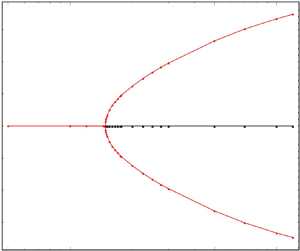
The lift-force equilibria identified above are plotted as a function of $Re_c$ in figure 5, the resulting locus conforming to a supercritical pitchfork bifurcation; the red dots and black triangles correspond to stable and unstable equilibria, respectively. Thus the central branch of the pitchfork corresponds to the centreline equilibrium that is stable for $Re_c \lesssim 148$, but unstable for larger $Re_c$. The two peripheral branches, consisting entirely of red dots, mark the emergence and subsequent wall-ward migration of the stable off-centre equilibria with increasing $Re_c$. The upper inset validates the square-root scaling expected in the neighbourhood of the bifurcation threshold defined by ${(Re_c-Re_c^{critical})}/{Re_c^{critical}} \ll 1$ ($Re_c^{critical} \approx 148$ as mentioned above). The lower inset shows the analogous bifurcation for a circular cylinder, with $Re_c \approx 110$ being the bifurcation threshold; the lower value of the threshold is consistent with the larger disturbance field, and the resulting stronger interaction with the walls, in two dimensions.

Figure 5. Equilibrium loci for a neutrally buoyant sphere and cylinder (lower inset) in plane Couette flow conforming to a supercritical pitchfork bifurcation; the vertical dashed lines denote $Re_c^{critical}$ for the two cases. The upper inset demonstrates the square-root scaling in the vicinity of the bifurcation threshold for the sphere; here, $\epsilon =({(Re_c-Re_c^{critical})}/{Re_c^{critical}})^{1/2}$.

While the bifurcation in figure 5 is similar to that in figure 6 of Fox et al. (2021), there is a key distinction that needs emphasis – the emergence of the bifurcation within a point-particle formulation, valid for small but finite $Re_p$, shows clearly that it corresponds to a critical $Re_c$, not $Re_p$. Since $Re_p=\lambda ^2\,Re_c$, the bifurcation can occur for arbitrarily small $Re_p$, provided that the confinement ratio is sufficiently small. The existence of the bifurcation in a point-particle formulation also implies that it likely owes its origin to a qualitative change in the disturbance velocity field on length scales larger than $a\,Re_p^{-({1}/{2})}$ – a change that likely results in a sphere at the centreline experiencing a net attractive interaction with its wall-induced images beyond $Re_c \approx 148$.

6. Conclusion

In this paper, we have calculated the lift velocity of a freely rotating neutrally buoyant sphere suspended in wall-bounded plane Couette flow, in the limit $Re_p\ll 1$, with $Re_c$ being arbitrary. Following Ho & Leal (1974), a generalized reciprocal theorem was used to calculate the lift velocity in the limit $Re_c\ll 1$, with the resulting profile exhibiting good agreement with the calculation of Vasseur & Cox (1976). For $Re_c\gtrsim O(1)$, the lift was obtained using a shooting method to solve the boundary value problem for the partial Fourier transform of the normal velocity and pressure fields obtained from the linearized Navier–Stokes equations. The numerical results reveal the channel centreline to be the only (stable) equilibrium for $Re_c \lesssim 148$, with a supercritical pitchfork bifurcation creating a pair of stable equilibria, on either side of the centreline, for larger $Re_c$; the analogous bifurcation for a circular cylinder occurs for $Re_c \approx 110$. The $Re_p$ thresholds for these two cases are $Re^{{critical}}_p \approx 148\lambda ^2$ and $110\lambda ^2$, implying that the threshold $Re_p$ can be arbitrarily small for sufficiently small $\lambda$. The analogous lift calculation for plane Poiseuille flow (Schonberg & Hinch 1989; Asmolov 1999; Anand & Subramanian 2023b), within a point-particle formulation, reveals no change in the number of equilibria with increasing $Re_c$; as first shown by Schonberg & Hinch (1989), the original pair of equilibria corresponding to the Segre–Silberberg pinch move towards the walls. It is thus interesting to note that the addition of ambient profile curvature actually simplifies the inertial migration problem! Further, our calculation, together with the emergence of an inner equilibrium in plane (Anand & Subramanian 2023a) and pipe (Matas, Morris & Guazzelli 2004; Nakayama et al. 2019) Poiseuille flow, due to finite-size effects, points to a potentially rich equilibrium landscape for a sphere in Couette–Poiseuille flow.

The point-particle formulation here predicts only the bifurcation curve in the limit $\lambda \to 0$. Thus the locus of equilibrium positions in figure 5 must be interpreted as the projection, onto the plane $\lambda = 0$, of a bifurcation surface in $s_{eq}$–$Re_c$–$\lambda$ space. Some idea of the nature of this surface may be obtained from the results of Fox et al. (2020, 2021). In the latter article, $Re_c^{critical}$ is found to increase from $30$ to $44$, and then to $70$, as $\lambda$ increases from $0.1$ to $0.15$ to $0.2$. Note that $Re_c^{critical}$ for the smallest $\lambda$ ($=0.1$) is far smaller than the threshold value (${\approx }148$) found here, suggesting an extremely steep decrease in the threshold as $\lambda$ increases to finite values. This pronounced sensitivity to $\lambda$ is very likely spurious, and a result of the coarse resolution along the $Re_c$-axis, in the said simulations. This is also inferred readily from the shapes of the pitchforks found in the simulations, which do not conform to the expected square-root scaling. The less expensive simulations for a cylinder (Fox et al. 2020), with a better $Re_c$ resolution (although not enough to recover the square-root scaling), do suggest an initial modest decrease, followed by a subsequent increase, in $Re_c^{critical}$ with increasing $\lambda$; the results for a cylinder also suggest a narrowing of the pitchfork with increasing $\lambda$. The sketch in figure 6 is a tentative depiction of the bifurcation surface based on the evidence above, and it is hoped that more comprehensive computations will delineate this surface in more detail.

Figure 6. A tentative sketch of the bifurcation surface in $s_{eq}$–$Re_c$–$\lambda$ space.

Extending the locus of equilibrium positions in figure 5 to higher $Re_c$ will be limited by two factors. The first is finite-size effects, which will need to be taken into account once the off-centre equilibria move sufficiently close to the wall, where one expects the resistance in the thin lubricating layer between the particle and the wall to retard and eventually arrest the wall-ward migration. The second factor is the transition to turbulence, which takes precedence over finite-size effects for sufficiently small $\lambda$. This transition is subcritical, being triggered by finite-amplitude perturbations, and known to occur for $Re_c \approx 1300\unicode{x2013}1500$ (Lundbladh & Johansson 1991; Tillmark & Alfredsson 1992; Dauchot & Daviaud 1995; Bottin & Chaté 1998; Lemoult et al. 2016). Not too far above the transition threshold, one expects the off-centre inertial equilibria to be smeared out into bands of a width determined by the amplitude of turbulent fluctuations. For a suspension of spherical particles in the turbulent regime, one expects a local peak in the volume fraction profiles sufficiently near the walls, on account of the underlying inertial equilibria, a feature that seems to have been observed in simulations (Wang, Abbas & Climent 2017), although one cannot rule out excluded volume effects as also playing a role. Weak turbulent fluctuations may also play a role in ‘equipartitioning’ spherical particles among the pair of off-centre equilibria, starting from an arbitrary initial distribution along the transverse channel coordinate; stochastic position fluctuations arising from inter-particle hydrodynamic interactions may play an analogous role, in the dilute limit, in the laminar regime. The analogous role of stochastic orientation fluctuations, in the context of suspension rheology, has been examined recently (Dabade, Marath & Subramanian 2016; Marath & Subramanian 2017, 2018; Marath, Dwivedi & Subramanian 2017).

One may also comment on the implications for anisotropic particles, specifically spheroids. It has been shown recently that the Jeffery-orbit-averaged lift velocity profile for neutrally buoyant spheroids differs from that for spheres by only a proportionality factor that is a function of the Jeffery orbit constant $C$ and the spheroid aspect ratio (Anand & Subramanian 2023b), therefore the equilibrium positions for spheroids in plane Poiseuille flow remain identical to those for a sphere. Since the Jeffery-orbit-averaged approximation is an accurate one for spheroids with aspect ratios of order unity, the Jeffery-averaged equilibrium locus, for a neutrally buoyant spheroid in plane Couette flow, should exhibit an identical bifurcation, with emergence of stable off-centreline equilibria above $Re_c \approx 148$. Note, however, that the rate of approach of a spheroid, from an arbitrary initial position to either of the off-centre equilibria, will depend on the aspect ratio, in general decreasing with increasing aspect ratio.

Finally, it is worth mentioning briefly the role of non-neutral buoyancy. There have been earlier calculations examining inertial migration of non-neutrally buoyant spheres, in plane Poiseuille flow, using a point-particle formulation (Hogg 1994; Asmolov 1999). A sphere in this framework is accounted for by a combination of Stokeslet and stresslet forcings, although only the former was included in the aforesaid efforts. The alignment of gravity relative to the shear flow now enters as an additional parameter, and the cases of flow- and vorticity-aligned gravity are of the most interest among the canonical ones; gradient-aligned gravity leads to an obvious departure from symmetry about the centreline. While the symmetric pitchfork bifurcation will be preserved in the vorticity-aligned case, the lift force arising for the flow-aligned case, which has been analysed in the limit of an unbounded simple shear flow by Saffman (1965) and McLaughlin (1991), will lead to a broken pitchfork bifurcation. Our preliminary calculations show that the resulting imperfect bifurcation consists of a continuous branch and an additional pair of equilibria that emerge beyond a threshold $Re_c$, via a saddle-node bifurcation, with this threshold being an increasing function of the departure from neutral buoyancy. These results, and their connection to the broken bifurcation scenario identified in the simulations of Fox et al. (2021), will be reported separately.