Universal law of skin-friction coefficient in a fully developed zero pressure gradient axisymmetric turbulent boundary layer flow

Abstract

Understanding the skin friction in an axisymmetric turbulent boundary layer (ATBL) flow is a key to designing and optimising the flow past axisymmetric bodies, for example, a rocket engine nozzle and a submarine hull. In this study, we propose a universal law of the skin-friction coefficient in an ATBL flow. The flow is steady and fully developed with a zero pressure gradient. The governing equation for the ATBL flow is derived by methodically applying the boundary layer approximation. Subsequently, the scaling law of the Reynolds shear stress, caused by turbulent eddies, at the surface tangential to the wall roughness summits is derived by incorporating the role of transverse curvature. The skin-friction coefficient in a smooth ATBL flow is found to depend on two parameters, namely, the Reynolds number based on the cylinder radius, Re_a, and the ratio of boundary layer thickness to cylinder radius, δ/a. The analysis predicts a simple form of the skin-friction coefficient as ${C_f} = 4.56 \times {10^{ - 2}}{[R{e_a}\ln (1 + \delta /a)]^{ - 1/4}}$, which agrees satisfactorily with the available experimental data and the numerical simulations in all the axisymmetric flow regimes. The proposed law, in the limit of infinite radius, is consistent with the classical law of the skin-friction coefficient in a plane turbulent boundary layer flow as ${C_{f0}}\sim Re_\delta ^{ - 1/4}$, where Re_δ is the Reynolds number based on the boundary layer thickness. This study reveals that, for δ/a < 1, the relative skin-friction coefficient, $({C_f} - {C_{f0}})/{C_{f0}}$, follows a linear law with δ$/$a.

1. Introduction

1.1. Problem statement

The main goal of this study is to obtain a universal law of the skin-friction coefficient in a steady and fully developed axisymmetric turbulent boundary layer (ATBL) flow with a zero pressure gradient. The surface drag experienced by an axisymmetric object, say a rocket engine nozzle or a submarine hull, is of considerable importance because of its tremendous impact on the overall system performance. Understanding the skin friction in an ATBL flow is therefore crucial for designing and optimising the flow past axisymmetric objects. By reducing the skin friction, the drag force can be minimised, resulting in an enhanced system performance.

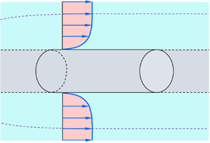
In an ATBL flow, the flow is rotationally symmetric around a central axis. The ATBL develops along an axisymmetric body, say flow past a cylinder with its axis aligned along the flow (figure 1). Let the cylinder radius be a, the boundary layer thickness be δ and the free stream velocity be U_∞. For a fully developed flow (δ no longer depends on the longitudinal distance z) with a zero pressure gradient, the dimensional analysis allows us to express the skin-friction coefficient C_f as follows:

(1.1)\begin{equation}{C_f} \equiv \frac{{{\tau _0}}}{{{\textstyle{1 \over 2}}\rho U_\infty ^2}} = f\left( {R{e_a},\frac{\delta }{a}} \right),\end{equation}

where $\tau_0$ is the wall shear stress, ρ is the mass density of fluid, f is the functional form, Re_a = U_∞a $/ \upsilon$ is the Reynolds number based on the cylinder radius and $\upsilon$ is the coefficient of kinematic viscosity of fluid. The objective of this study is to find the functional form (1.1) by means of a theoretical approach. Since an analytical formula is simpler and computationally more efficient than the numerical techniques, the proposed formula would be easier to use and more accessible to researchers.

Figure 1. Flow past an axisymmetric body, say a rigid cylinder with a radius a, described with respect to a cylindrical coordinate system (r, θ, z). Here, ū_z is the time-averaged longitudinal velocity in the z direction, ${U_\infty } = {\bar{u}_z}{|_{r \,=\, a \,+\, \delta }}$ is the free stream velocity, δ is the boundary layer thickness, r = a defines the surface of the cylinder and r = a + δ defines the edge of the ATBL.

1.2. The ATBL flow regimes

A plane turbulent boundary layer (TBL) flow is characterised by two length scales, namely, the boundary layer thickness δ and the viscous length scale $\upsilon / $u_*, where ${u_\ast } = {({\tau _0}/\rho )^{1/2}}$ is the friction velocity. However, an ATBL flow possesses an extra length scale, that is, the radius of transverse curvature a. The role of transverse curvature in an ATBL flow has long been studied experimentally (Richmond 1957; Yu 1958; Rao 1967; Chase 1972; Rao & Keshavan 1972; Patel, Nakayama & Damian 1974; Willmarth et al. 1976; Luxton, Bull & Rajagopalan 1984; Lueptow, Leehey & Stellinger 1985; Cipolla & Keith 2003; Krane, Grega & Wei 2010). The additional length scale in an ATBL flow gives rise to three different flow regimes depending on two dimensionless parameters. They are the ratio of boundary layer thickness to radius of curvature, δ $/$a, and the dimensionless radius of curvature (in wall units), ${a^ + } = a{u_\ast }/\upsilon$. The classification of flow regimes can be found in the work of Piquet & Patel (1999), Woods (2006) and Kumar & Mahesh (2018a). However, for the convenience of the readers, the flow regimes are briefly summarised below.

1. (i) Regime I (δ/a ≤ 1 and a ⁺ > 250): in this flow regime, the effect of the transverse curvature on the flow is negligible. The flow behaves as if it were a plane TBL flow. However, it offers an increased skin friction compared with a plane TBL flow having the same Reynolds number based on the boundary layer thickness, $R{e_\delta } = {U_\infty }\delta /\upsilon$. Using the matched asymptotic expansion method, Afzal & Narasimha (1976) showed that, for δ/a = O(1) and large a ⁺, the longitudinal velocity distribution ū_z(y) in the viscous sublayer is expressed as

   (1.2)\begin{equation}u_z^ += {a^ + }\ln \left( {1 + \frac{y}{a}} \right),\end{equation}
   whereas that in the logarithmic layer follows the axisymmetric logarithmic law as
   (1.3)\begin{equation}u_z^ += \frac{1}{\kappa }\ln \left[ {{a^ + }\ln \left( {1 + \frac{y}{a}} \right)} \right] + B.\end{equation}

In (1.2) and (1.3), $u_{z}^{+} = \bar{u}_{z}/u_{\ast}$, y is the wall-normal distance measured from the surface of the cylinder, κ is the von Kármán constant (that is, the slope of the axisymmetric logarithmic law) and B is the intercept. Afzal & Narasimha (1976) found that B is a weak function of the transverse curvature as B = 5 + 236$/$a ⁺.

1. (ii) Regime II (δ/a > 1 and a ⁺ > 250): in this flow regime, the effect of the curvature is sensed only in the outer flow layer. The velocity distribution preserves a logarithmic layer described by (1.3), having a decreasing slope (Lueptow et al. 1985).

2. (iii) Regime III (δ $/$a > 1 and a ⁺ < 250): in this flow regime, the effect of the strong curvature influences both the inner and outer flow layers. The logarithmic layer decays and turns out to be negatively curved (Willmarth et al. 1976; Luxton et al. 1984).

Nearly all experimental studies paid attention to the last two flow regimes (regimes II and III). However, the availability of the experimental data for these flow regimes has been limited. This is because, to achieve a large δ $/$a, experiments were generally conducted using either a long tube or a wire having a small diameter. Therefore, the structural isolation of wires and the aeroelastic interaction between the wire and the flow had caused major issues. Moreover, in a typical experimental set-up, it was rather challenging to maintain the alignment of the cylinder with the flow and to prevent the sagging of the cylinder due to the elastic deformation (Piquet & Patel 1999). Furthermore, for a small a ⁺, the measuring probe size with respect to the cylinder radius has been a serious concern in taking measurements close to the wall. To avoid such difficulties, researchers studied the problem extensively by means of numerical simulations (Neves, Moin & Moser 1994; Tutty 2008; Jordan 2011, 2013, 2014a,b; Monte, Sagaut & Gomez 2011). The results of the direct numerical simulation (DNS) (Neves et al. 1994; Woods 2006; Tutty 2008), large eddy simulation (LES) (Jordan 2011, 2013) and axisymmetric Reynolds-averaged Navier–Stokes (RANS) (Monte et al. 2011) provided deeper understanding of the skin-friction coefficient over a considerable range of the parameter space.

1.3. Empirical formulae of skin-friction coefficient

The skin-friction coefficient can be obtained from (1.3) if the axisymmetric logarithmic law is preserved throughout the boundary layer. Although there have been efforts to identify the effect of the transverse curvature on the logarithmic law of the velocity distribution, a generic consensus is still lacking in this regard. The logarithmic law, involving the slope and intercept parameters κ and B, respectively, is expected to depend on the radius of curvature (Willmarth et al. 1976; Luxton et al. 1984). For example, Rao & Keshavan (1972) proposed that the slope parameter κ is a function of Re_a only, whereas the intercept parameter B is a function of both Re_a and a ⁺.

Woods (2006) found that (1.3), with κ = 0.4 and B = 5.1, captures the velocity distribution in the ATBL flows. Using $U_{\infty}=\bar{u}_{z}\ (y=\delta)$, (1.3) gives

(1.4)\begin{equation}\frac{{{U_\infty }}}{{{u_\ast }}} = 2.5\ln \left[ {{a^ + }\ln \left( {1 + \frac{\delta }{a}} \right)} \right] + 5.1.\end{equation}

Using ${C_f} = 2u_\ast ^2/U_\infty ^2$ and ${a^ + } = R{e_a}\sqrt {{C_f}/2} $, (1.4) is rearranged as

(1.5)\begin{equation}\sqrt {\frac{2}{{{C_f}}}} + 2.5\ln \sqrt {\frac{2}{{{C_f}}}} = 2.5\ln \left[ {R{e_a}\ln \left( {1 + \frac{\delta }{a}} \right)} \right] + 5.1,\end{equation}

which can be solved for the given Re_a and δ $/$a. Figure 2 shows the numerical solution of (1.5), herein called the axisymmetric logarithmic solution, by plotting $\sqrt {2/{C_f}} $ as a function of $R{e_a}\ln (1 + \delta /a)$. As the analytical solution of (1.5) is not straightforward, Woods (2006) neglected the slowly evolving function $\ln \sqrt {2/{C_f}} $ and proposed a reduced form of (1.5) as follows:

(1.6)\begin{equation}\sqrt {\frac{2}{{{C_f}}}} = {A_0}\ln \left[ {R{e_a}\ln \left( {1 + \frac{\delta }{a}} \right)} \right] + {B_0},\end{equation}

where A ₀ and B ₀ are the fitting parameters. Using the available experimental data and the DNS data, Woods (2006) found A ₀ = 2.97 and B ₀ = −5.82. Woods’ (2006) empirical formula (1.6) is also plotted in figure 2. The axisymmetric logarithmic solution departs from Woods’ (2006) empirical formula. The reason is that, in (1.5), the slope and the intercept parameters of the axisymmetric logarithmic law are kept constant, although they are expected to vary with the curvature (Rao & Keshavan 1972).

Figure 2. Comparison of the skin-friction coefficients obtained from the axisymmetric logarithmic solution and Woods’ (2006) empirical formula.

Monte et al. (2011) used an axisymmetric RANS formulation and adjusted the fitting parameters of (1.6) as A ₀ = 2.56 and B ₀ = −2.53. They also performed the nonlinear fitting of their simulation data and proposed the following empirical form:

(1.7)\begin{equation}{C_f} = \exp [G(\ln R{e_a};\ln R{e_\delta })],\end{equation}

where G(β; γ) is a third-order polynomial function. It is given by $G(\beta ;\gamma ) = {a_0} + {a_1}\beta + {a_2}{\beta ^2} + {a_3}{\beta ^3} + {a_4}\beta \gamma + {a_5}\beta {\gamma ^2} + {a_6}{\beta ^2}\gamma + {a_7}{\gamma ^3} + {a_8}{\gamma ^2} + {a_9}\gamma$, where a ₀ to a ₉ are the coefficients.

Jordan (2013, 2014b) proposed models for the skin-friction coefficient in an ATBL flow. The LES results of Jordan (2011, 2013) offered an enhanced understanding of the ATBL flow properties over considerable ranges of Re_a and δ $/$a.

Among recent studies, Kumar & Mahesh (2018a) performed an insightful analysis of a developing ATBL flow using the momentum integral approach. The mathematical analysis could capture the effects of the pressure gradient and the transverse curvature on the skin-friction coefficient. The proposed analytical relations were in satisfactorily agreement with the experimental data of the skin-friction coefficient for a developing ATBL flow. Kumar & Mahesh (2018b) and Morse & Mahesh (2021) presented the LES results of flow over an idealised submarine hull, providing enhanced understanding of the skin-friction coefficient along the axisymmetric body. Balantrapu et al. (2021) experimentally studied the highly decelerated ATBL flow over a body of revolution, focussing on the mean flow, turbulence statistics and the skin-friction coefficient.

Despite magnificent advances on the ATBL flow, a universal law of the skin-friction coefficient, even for a simplified flow configuration (steady and fully developed ATBL flow with a zero pressure gradient), has remained unexplored from a theoretical perspective. The empirical formulae of the skin-friction coefficient in an ATBL flow contain free parameters, which were obtained from the regression analyses of the available experimental and/or simulation data. The empirical formulae work satisfactorily over a wide range of the parameter space. However, as these formulae were developed on the empirical ground, they lack theoretical support. In this study, we seek a universal scaling law of the skin-friction coefficient in an ATBL flow. The governing equation for a steady and fully developed ATBL flow with a zero pressure gradient is derived systematically starting from the axisymmetric equations followed by Reynolds averaging and the boundary layer approximation. Then, the scaling law of the Reynolds shear stress caused by near-wall turbulent eddies is derived. This allows us to obtain the wall shear stress and subsequently provides an estimation of the skin-friction coefficient.

The rest of the paper is organised as follows. The theoretical analysis is described in § 2. In § 3, the theoretical results, including the compatibility of the proposed law with the classical law of the skin-friction coefficient in a plane TBL flow, comparison with previous work and some important scaling aspects, are thoroughly discussed. Finally, conclusions are drawn in § 4.

2. Theoretical analysis

2.1. Governing equations

In an axisymmetric flow (figure 1), the flow parameters with respect to a cylindrical coordinate system (r, θ, z) are invariant with the azimuthal angle θ, that is, ∂(⋅)/∂θ = 0. Therefore, on a given (r, θ) plane, any flow parameter remains unchanged along a circle of constant radius. For an incompressible ATBL flow, the continuity equation and the steady-state Navier–Stokes equations devoid of the body force terms are expressed as (see, for instance, Pope 2000)

(2.1)\begin{gather}\frac{1}{r}\frac{{\partial r{u_r}}}{{\partial r}} + \frac{{\partial {u_z}}}{{\partial z}} = 0,\end{gather}

(2.2)\begin{gather}{u_r}\frac{{\partial {u_z}}}{{\partial r}} + {u_z}\frac{{\partial {u_z}}}{{\partial z}} =- \frac{1}{\rho }\frac{{\partial p}}{{\partial z}} + \upsilon {\nabla ^2}{u_z},\end{gather}

(2.3)\begin{gather}{u_r}\frac{{\partial {u_r}}}{{\partial r}} - \frac{{u_\theta ^2}}{r} + {u_z}\frac{{\partial {u_r}}}{{\partial z}} =- \frac{1}{\rho }\frac{{\partial p}}{{\partial r}} + \upsilon \left( {{\nabla^2}{u_r} - \frac{{{u_r}}}{{{r^2}}}} \right),\end{gather}

where u_r, u_θ and u_z are the velocity components in the radial (r), azimuthal (θ) and longitudinal (z) directions, respectively, and p is the pressure. In (2.2) and (2.3), the operator ∇² is given by

(2.4)\begin{equation}{\nabla ^2} = \frac{1}{r}\frac{\partial }{{\partial r}}\left( {r\frac{\partial }{{\partial r}}} \right) + \frac{{{\partial ^2}}}{{\partial {z^2}}}.\end{equation}

Under the assumption of a statistically stationary flow with no swirl motion, the instantaneous velocity components and pressure, according to the Reynolds decomposition, are expressed as $u_{r}=\bar{u}_{r}+ u_{r}^{\prime}, u_\theta = {u^{\prime}_\theta }, u_{z}=\bar{u}_{z}+u_{z}^{\prime}$ and $p = \bar{p} + p^{\prime}$. Here, an overbar denotes a statistically time-averaged quantity and a prime denotes the fluctuation of an instantaneous quantity with respect to its time-averaged value. Performing the time averaging, the continuity and the momentum equations, (2.1)–(2.3), give the time-averaged continuity and the RANS equations for an ATBL flow as follows:

(2.5)\begin{gather}\frac{1}{r}\frac{{\partial r{{\bar{u}}_r}}}{{\partial r}} + \frac{{\partial {{\bar{u}}_z}}}{{\partial z}} = 0,\end{gather}

(2.6)\begin{gather}{\bar{u}_r}\frac{{\partial {{\bar{u}}_z}}}{{\partial r}} + {\bar{u}_z}\frac{{\partial {{\bar{u}}_z}}}{{\partial z}} =- \frac{1}{\rho }\frac{{\partial \bar{p}}}{{\partial z}} + \upsilon \left[ {\frac{1}{r}\frac{\partial }{{\partial r}}\left( {r\frac{{\partial {{\bar{u}}_z}}}{{\partial r}}} \right) + \frac{{{\partial^2}{{\bar{u}}_z}}}{{\partial {z^2}}}} \right] - \frac{1}{r}\frac{{\partial r\overline {{u^{\prime}_r}{u^{\prime}_z}} }}{{\partial r}} - \frac{{\partial \overline {{u^{\prime}_z}{u^{\prime}_z}} }}{{\partial z}},\end{gather}

(2.7)\begin{gather}{\bar{u}_r}\frac{{\partial {{\bar{u}}_r}}}{{\partial r}} + {\bar{u}_z}\frac{{\partial {{\bar{u}}_r}}}{{\partial z}} =- \frac{1}{\rho }\frac{{\partial \bar{p}}}{{\partial r}} + \upsilon \left[ {\frac{1}{r}\frac{\partial }{{\partial r}}\left( {r\frac{{\partial {{\bar{u}}_r}}}{{\partial r}}} \right) + \frac{{{\partial^2}{{\bar{u}}_r}}}{{\partial {z^2}}} - \frac{{{{\bar{u}}_r}}}{{{r^2}}}} \right] - \frac{1}{r}\frac{{\partial r\overline {{u^{\prime}_r}{u^{\prime}_r}} }}{{\partial r}}\notag\\ - \frac{{\partial \overline {{u^{\prime}_r}{u^{\prime}_z}} }}{{\partial z}} + \frac{{\overline {{u^{\prime}_\theta }{u^{\prime}_\theta }} }}{r}.\end{gather}

The expressions (2.6) and (2.7) show that, in a statistically stationary non-swirling axisymmetric flow, only the term $\overline {{u^{\prime}_r}{u^{\prime}_z}} $ contributes to the Reynolds shear stress. Among the Reynolds normal stresses, only the longitudinal Reynolds normal stress $\overline {{u^{\prime}_z}{u^{\prime}_z}} $ contributes to the longitudinal momentum balance, whereas the radial and azimuthal Reynolds normal stresses, $\overline {{u^{\prime}_r}{u^{\prime}_r}} $ and $\overline {{u^{\prime}_\theta }{u^{\prime}_\theta }} $, respectively, contribute to the radial momentum balance. The quantity $\overline {{u^{\prime}_\theta }{u^{\prime}_\theta }} $ in (2.7) remains finite because of the non-zero azimuthal velocity fluctuations, although the time-averaged azimuthal velocity is zero (ū_θ = 0).

2.2. The ATBL approximation

Applying the ATBL approximation (for detailed derivation, see Appendix A), (2.6) and (2.7) reduce to

(2.8)\begin{gather}{\bar{u}_r}\frac{{\partial {{\bar{u}}_z}}}{{\partial r}} + {\bar{u}_z}\frac{{\partial {{\bar{u}}_z}}}{{\partial z}} =- \frac{1}{\rho }\frac{{\partial \bar{p}}}{{\partial z}} + \upsilon \frac{1}{r}\frac{\partial }{{\partial r}}\left( {r\frac{{\partial {{\bar{u}}_z}}}{{\partial r}}} \right) - \frac{1}{r}\frac{{\partial r\overline {{u^{\prime}_r}{u^{\prime}_z}} }}{{\partial r}},\end{gather}

(2.9)\begin{gather}0 =- \frac{1}{\rho }\frac{{\partial \bar{p}}}{{\partial r}} - \frac{1}{r}\frac{{\partial r\overline {{u^{\prime}_r}{u^{\prime}_r}} }}{{\partial r}} + \frac{{\overline {{u^{\prime}_\theta }{u^{\prime}_\theta }} }}{r}.\end{gather}

The integration of (2.9) gives the pressure distribution as

(2.10)\begin{equation}\bar{p} = {\bar{p}_\infty }(z) + \rho {\overline {{u^{\prime}_r}{u^{\prime}_r}} } |_r^\delta + \rho \int_r^\delta {\left( {\frac{{\overline {{u^{\prime}_r}{u^{\prime}_r}} - \overline {{u^{\prime}_\theta }{u^{\prime}_\theta }} }}{r}} \right)\,\textrm{d}r} ,\end{equation}

where ${\bar{p}_\infty }$ is the time-averaged pressure at the edge of the boundary layer, that is, the free stream pressure. In (2.10), the difference between the radial and azimuthal Reynolds normal stresses, $\overline {{u^{\prime}_r}{u^{\prime}_r}} - \overline {{u^{\prime}_\theta }{u^{\prime}_\theta }} $, remains finite if the turbulence is statistically anisotropic $(\overline {{u^{\prime}_r}{u^{\prime}_r}} \ne \overline {{u^{\prime}_\theta }{u^{\prime}_\theta }} )$. Therefore, in an anisotropic turbulence, the quantity $\overline {{u^{\prime}_r}{u^{\prime}_r}} - \overline {{u^{\prime}_\theta }{u^{\prime}_\theta }} $ contributes to the pressure distribution. However, in an isotropic turbulence, the last term on the right-hand side of (2.10) vanishes.

Substituting (2.10) into (2.8) gives

(2.11)\begin{align}{\bar{u}_r}\frac{{\partial {{\bar{u}}_z}}}{{\partial r}} + {\bar{u}_z}\frac{{\partial {{\bar{u}}_z}}}{{\partial z}} =- \frac{1}{\rho }\frac{{\textrm{d}{{\bar{p}}_\infty }}}{{\textrm{d}z}} - \frac{{\partial {\overline {{u^{\prime}_r}{u^{\prime}_r}} } |_r^\delta }}{{\partial z}} - \frac{\partial }{{\partial z}}\int_r^\delta {\left( {\frac{{\overline {{u^{\prime}_r}{u^{\prime}_r}} - \overline {{u^{\prime}_\theta }{u^{\prime}_\theta }} }}{r}} \right)\,\textrm{d}r} + \frac{1}{{\rho r}}\frac{{\partial r\tau }}{{\partial r}},\end{align}

where τ is the total shear stress (= $\tau_v$ + $\tau_t$), that is, the sum of the viscous shear stress, $\tau_{v}$ = ρ $\upsilon$∂ū_z/∂r and the Reynolds shear stress, ${\tau _t} =- \rho \overline {{u^{\prime}_r}{u^{\prime}_z}} $.

2.3. Fully developed ATBL flow with a zero pressure gradient

In a fully developed ATBL flow, the flow parameters do not evolve in the longitudinal direction, that is, ∂(⋅)$/$∂z = 0. Since ∂ū_z $/$∂z = 0 (that is, ū_z is a function of r only) because of the fully developed flow, the continuity demands rū_r = F(z) + c ₁ (by virtue of (2.5)), where c ₁ is a constant. However, the function F(z) must be a constant, because ū_r should also remain invariant with z to satisfy the fully developed flow. This can also be concluded by setting ∂ū_r $/$∂z = 0, which gives F′(z) = 0 (that is, F(z) is a constant). Letting F(z) = c ₂ (c ₂ is a constant), we obtain ū_r = c ₃/r with c ₃ = c ₁ + c ₂. As the radial velocity vanishes at the wall due to the no-slip boundary condition, the condition ū_r (r = a) = 0 predicts c ₃ = 0, which eventually results in ū_r = 0. Therefore, in a fully developed ATBL flow, the convective acceleration in the longitudinal momentum equation vanishes (left-hand side of (2.11)). In addition, the second and third terms on the right-hand side of (2.11) become zero. However, the longitudinal pressure gradient and the radial gradient of the total shear stress remain non-zero. This shows that the total shear stress varies radially to balance the longitudinal free stream pressure gradient. For the zero pressure gradient flow, it gives $\textrm{d}{\bar{p}_\infty }/\textrm{d}z = 0$. Hence, in a fully developed ATBL flow with a zero pressure gradient, all barring the last term on the right-hand side of (2.11) are zero. As a result, (2.11) recovers the equilibrium model of, among others, Glauert & Lighthill (1955) and Rao (1967). This indicates the moment of the total shear stress to be a constant (rτ = constant). The constant is obtained from the boundary condition τ(r = a) = $\tau_0$. Thus, (2.11) reduces to

(2.12)\begin{equation}r\tau = a{\tau _0}.\end{equation}

It is worth mentioning that the relationships (1.2) and (1.3) can be recovered from (2.12). In this regard, we set the outward wall-normal distance as y = r − a. In the near-wall flow region, $\tau_t$ vanishes within the thin viscous sublayer, resulting in τ = $\tau_v$. Substituting $\tau_v$ = ρ $\upsilon\,$dū_z $/$dy into (2.12) and integrating the resultant equation by applying the no-slip boundary condition ū_z (r = a) = 0 yield (1.2). In fact, (1.2) resembles the linear law of the wall in a plane TBL flow given by $u_z^ += {y^ + }$ (where ${y^ + } = y{u_\ast }/\upsilon$) (see, for instance, Ali & Dey 2020), if the term a ln (1 + y/a) is replaced by y. In the logarithmic layer, $\tau_v$ becomes zero and τ = $\tau_t$. Therefore, (2.12) suggests an inverse scaling of $\tau_t$ with y, in conformity with the experimental measurements (Lueptow et al. 1985). Analogously to the mixing length hypothesis in a plane TBL flow, $\tau_t$ in an ATBL flow can be expressed as $\tau_{t} = \rho l^{2}_{p} ({\rm d}\bar{u}_{z}/{\rm d}y)^{2}$, where l_p is the mixing length. From (2.12), it follows that $\textrm{d}{\bar{u}_{z}}/\textrm{d}y = [a/(a + y)]^{1/2} u_{\ast} l^{-1}_{p}$, which, upon integration, in association with ${l_p} = \kappa {[a(a + y)]^{1/2}}\ln (1 + y/a)$, produces (1.3). The present choice of l_p in the limit of infinite radius (a → ∞) is consistent with the classical expression l_p = κy in the logarithmic layer of a plane TBL flow (Schlichting 1979). The relation (1.3) is analogous to the logarithmic law in a plane TBL flow, given the term a $\ln$(1 + y $/$a) is exchanged with y.

2.4. Scaling law of Reynolds shear stress

It is pertinent to mention that the present analysis aims at deriving the skin-friction coefficients for both the rough and smooth ATBL flows. However, due to the absence of experimental data on the skin-friction coefficient, specifically in a rough ATBL flow, the experimental verification of the proposed skin-friction coefficient is limited to the smooth ATBL flow data only (see § 3.2). The mathematical analysis starts with a rough wall configuration to establish a scaling law of the skin-friction coefficient. Subsequently, the skin-friction coefficient in a smooth ATBL flow is derived using this scaling law. We now intend to derive the scaling law of the Reynolds shear stress $\tau_t$ acting on the rough wall of the cylinder. The wall roughness is of k-type, where the surface of the cylinder is covered with a layer of closely packed identical particles of diameter k_s, called the roughness height (see the enlarged view shown in figure 3). At a microscopic level, an undulating surface is formed above y = 0 (that is, r = a). The bulk flow Reynolds number is sufficiently large, so that the viscous shear stress is negligible, and the total shear stress includes only the Reynolds shear stress. The value of $\tau_t$ is sought at the hypothetical surface S tangential to the roughness summits, given by y = k_s $/$2 (that is, r = a + k_s $/$2). Consequently, the wall shear stress from (2.12) is obtained as

(2.13)\begin{equation}{\tau _0} = \left( {1 + \frac{{{k_s}}}{{2a}}} \right){\tau _t}.\end{equation}

Figure 3. The Reynolds shear stress $\tau_t$ developed at the surface S (tangential to the roughness summits) caused by a turbulent eddy of size ℓ straddling the surface and exchanging the momentum across S. The turbulent eddy carries high- and low-momentum fluid per unit volume inwards and outwards, respectively, across S. The value of $\tau_t$ is obtained from the product of the momentum contrast per unit volume across S and the eddy turnover velocity u_ℓ as ${\tau _t} = \rho ({\bar{u}_z}{|_{y \,=\, {k_s}/2 \,+\, \ell /2}} - {\bar{u}_z}{|_{y \,=\, {k_s}/2 \,-\, \ell /2}}){u_\ell }$.

The Reynolds shear stress in a turbulent flow is caused by turbulent eddies of various length scales. The largest eddy size is comparable to the external length scale of the system. As discussed in the preceding section, the preservation of the law of the wall in an ATBL flow requires the wall-normal distance y in a plane TBL flow to be replaced by a $\ln$(1 + y $/$a). For a given a, y is always larger than a $\ln$(1 + y $/$a). This reveals that any wall-normal length scale in a plane TBL flow experiences a length contraction in an ATBL flow because of the transverse curvature. Let the boundary layer thickness be the same, say δ, for both the ATBL and plane TBL flows. The external length scale $\mathscr{L}$ (that is, the largest eddy size) in a plane TBL flow is thus $\mathscr{L}$ ~ δ. However, due to the length contraction, $\mathscr{L}$ in an ATBL flow becomes smaller than that in a plane TBL flow. Following the length contraction in an ATBL flow, $\mathscr{L}$ takes the form of

(2.14)\begin{equation}\mathscr{L}\sim a\ln \left( {1 + \frac{\delta }{a}} \right),\end{equation}

which, for a given δ, is consistent with the classical expression $\mathscr{L}$ ~ δ in a plane TBL flow in the limit of infinite radius (a → ∞).

The Reynolds shear stress $\tau_t$ at S is developed by turbulent eddies that straddle the surface (eddies are bisected by the surface S) and exchange momentum across S. This mechanism was first applied by Gioia & Bombardelli (2002) to analyse the scaling and similarity in rough-channel flows (see, for instance, the review of Ali & Dey 2018). Beneath S, the flow velocity is negligible, because of the protruding wall roughness (figure 3). The momentum that the flow transmits tangential to S is thus insignificant. By contrast, above S, the flow transmits a substantial momentum tangential to S. It follows that a turbulent eddy of size ℓ carries high-momentum fluid per unit volume inwards (towards the cylinder) across S and low-momentum fluid per unit volume outwards (away from the cylinder) across S. Therefore, across S, the momentum contrast per unit volume produced by the turbulent eddy is $\rho(\bar{u}_{z}|_{y\,=\,k_{s}/2\,+\,\ell/2}- \bar{u}_{z}|_{y\,=\,k_{s}/2\,-\,\ell/2}) \approx \rho\ell(\textrm{d}\bar{u}_{z}/\textrm{d}y)|_{y\,=\,k_{s}/2}$. The rate of momentum exchange across S is caused by the eddy turnover velocity u_ℓ. The value of $\tau_t$ caused by a turbulent eddy of size ℓ is obtained as a product of the net momentum contrast per unit volume across S and u_ℓ. Therefore, $\tau_t$ is expressed as

(2.15)\begin{equation}{\tau _t} = \rho {\left. {\frac{{\textrm{d}{{\bar{u}}_z}}}{{\textrm{d}y}}} \right|_{y \,=\, {k_s}/2}}\ell {u_{\ell}}.\end{equation}

The velocity gradient in (2.15) is obtained from the differentiation of (1.3) as follows:

(2.16)\begin{equation}{\left. {\frac{{\textrm{d}{{\bar{u}}_z}}}{{\textrm{d}y}}} \right|_{y \,=\, {k_s}/2}} = \frac{{{u_\ast }}}{{\kappa a\left( {1 + \dfrac{{{k_s}}}{{2a}}} \right)\ln \left( {1 + \dfrac{{{k_s}}}{{2a}}} \right)}}.\end{equation}

The value of u_ℓ is obtained from the second-order transverse structure function as $u_\mathrm{\ell }^2 = S_2^ \bot (\mathrm{\ell })$, where $S_2^ \bot (\mathrm{\ell })$ is expressed as

(2.17)\begin{equation}S_2^ \bot (\mathrm{\ell }) = \overline{[{u^{\prime}_r}(z + \ell /2) - {u^{\prime}_r}(z - \ell /2) ]^2}.\end{equation}

It has been evidenced that, analogously to the second-order longitudinal structure function, given by

(2.18)\begin{equation}S_2^\parallel (\mathrm{\ell }) = \overline {[{u^{\prime}_z}(z + \ell /2) - {u^{\prime}_z}(z - \ell /2) ]^2},\end{equation}

$S_2^ \bot (\mathrm{\ell })$ obeys Kolmogorov's two-thirds law over a significant range (Frisch 1995). Dimensional argument produces

(2.19)\begin{equation}u_\mathrm{\ell }^2 \equiv {(\varepsilon \ell )^{2/3}}H\left( {\frac{\ell }{\mathscr{L}};Re} \right),\end{equation}

where ε is the turbulent kinetic energy (TKE) dissipation rate, Re is the Reynolds number based on the external length scale and ℓ is considered to lie in the inertial range. For a complete similarity in the variables ℓ $/\mathscr{L}$ and Re, the function H becomes constant as ℓ $/\mathscr{L}$  → 0 and Re → ∞, recovering Kolmogorov's two-thirds law, $u_\mathrm{\ell }^2\sim {(\varepsilon \ell )^{2/3}}$ for the limiting state of fully developed turbulence. However, as ℓ $/ \mathscr{L}$  → 0, the complete similarity breaks down because of the TKE dissipation rate fluctuations. Therefore, for an incomplete similarity, H does not approach a finite limit as ℓ $/ \mathscr{L}$  → 0. Under such circumstance, (2.19) takes the form of

(2.20)\begin{equation}u_\mathrm{\ell }^2 \equiv {(\varepsilon \ell )^{2/3}}H\left( {\frac{\ell }{\mathscr{L}};\ln Re} \right),\end{equation}

which is valid not only for a large Re but also for a large ln Re (Barenblatt & Goldenfeld 1995). For an incomplete similarity, as ℓ $/ \mathscr{L}$  → 0, (2.20) is expanded as

(2.21)\begin{equation}\left. \begin{array}{c@{}} u_\mathrm{\ell }^2 = {(\varepsilon \mathrm{\ell })^{2/3}}C(\ln Re){\left( {\dfrac{\mathrm{\ell}}{\mathscr{L}}} \right)^\alpha },\\ C(\ln Re) = {C_0} + \dfrac{{{C_1}}}{{\ln Re}} + O\left( {\dfrac{1}{{{{\ln}^2}\,Re}}} \right),\textrm{ }\\ \alpha = {\alpha_0} + \dfrac{{{\alpha_1}}}{{\ln Re}} + O\left( {\dfrac{1}{{{{\ln }^2}\,Re}}} \right), \end{array}\!\!\!\right\}\end{equation}

where C ₀ and C ₁ are the coefficients, and α ₀ and α ₁ are the exponents.

The expression (2.21) shows that, as the eddy size ℓ increases, its turnover velocity u_ℓ also increases and, subsequently, ℓu_ℓ increases. Therefore, $\tau_t$ at S enhances with an increase in ℓ, in accord with (2.15). The gathering of near-wall eddies that exchange momentum through S can be visualised as a set of circular fluid cells in two dimensions (or spheroidal fluid cells in three dimensions) between two successive roughness summits (figure 4a). The length scale ℓ of such eddies can be divided into two groups, such as ℓ ≤ ℓ_m and ℓ > ℓ_m (ℓ still lies in the inertial range), where ℓ_m is the maximum size of an eddy (that is, the presiding eddy) being bisected by the surface S. For ℓ < ℓ_m, the eddies are perfectly bisected by the surface S and, thereby, $\tau_t$ at S increases with ℓ (figure 4b). However, $\tau_t$ at S does not continue to increase persistently as ℓ increases. There remains an upper limit of ℓ (= ℓ_m) for which the presiding eddy maximises $\tau_t$ at S. For ℓ > ℓ_m, the eddies are not bisected by the surface S, because of the geometrical constraint produced by the wall roughness. These eddies contribute minimally to the shear stress generation due to their insignificant momentum exchanges across S. This suggests that the maximum $\tau_t$ at S is caused by the presiding eddy of size ℓ = ℓ_m. From the two-dimensional geometry (figure 4a), ℓ_m turns out to be ${\ell _m}\, = (\sqrt 2 - 1){k_s} \approx 0.414{k_s}$ (that is, ℓ_m is of the order of the roughness height). The maximum $\tau_t$ at S is obtained from (2.15) by setting ℓ = 0.414k_s. After some algebra, $\tau_t$ is expressed as follows:

(2.22)\begin{align}{\tau _t}&\sim \rho \frac{{{u_\ast }}}{{a\left( {1 + \dfrac{{{k_s}}}{{2a}}} \right)\ln \left( {1 + \dfrac{{{k_s}}}{{2a}}} \right)}}{k_s}{(\varepsilon {k_s})^{1/3}}{\left( {{C_0} + \frac{{{C_1}}}{{\ln Re}}} \right)^{1/2}}\nonumber\\&\quad \times \begin{bmatrix}\displaystyle\frac{{{k_s}}}{{a\ln \left( {1 + \dfrac{\delta }{a}} \right)}}\end{bmatrix}^{(\alpha _0 \,+\, \alpha _1/\ln Re)/2}. \end{align}

Figure 4. (a) Near-wall eddies having length scales ℓ < ℓ_m (green), ℓ = ℓ_m (blue) and ℓ > ℓ_m (red) exchanging momentum across the surface S. Here, ℓ_m is the maximum size of an eddy, called the presiding eddy (in blue), which is bisected by surface S. (b) Conceptual variation of $\tau_t$ with ℓ. The value of $\tau_t$ at S enhances with an increase in ℓ attaining a maximum at ℓ = ℓ_m and then decreases with a further increase in ℓ.

The value of ε in (2.22) can be inferred from the TKE budget equation, which defines the rate of conservation of the TKE through the mechanisms of advection, diffusion, dissipation and production. The diffusion rate comprises the TKE, pressure energy and viscous diffusion rates. In the near-wall flow region, say, in the logarithmic layer, the numerical simulations have evidenced that the key contributors to the TKE budget equation are the TKE production and dissipation rates (Woods 2006). Considering various ranges of a ⁺ (= 21 to 1124.9) and δ $/$a (= 0.16 to 27.6), Woods (2006) found the following ranges of the dimensionless TKE budget components (scaled by $u_\ast ^4/\upsilon $) at y ⁺ = 30: TKE production rate (0.03 to 0.08), TKE dissipation rate (0.02 to 0.08), TKE diffusion rate (0.012 to 0.016), pressure energy diffusion rate (0 to −1.3 × 10⁻³) and viscous diffusion rate (≈0). Therefore, in the absence of the TKE advection rate, the TKE production rate is balanced by the TKE dissipation rate. It follows that ε at S is obtained from the energy balance, $\varepsilon= P=(\tau_{t}/\rho)(\textrm{d}\bar{u}_{z}/\textrm{d}y)|_{y\,=\,k_{s}/2}$, where P is the TKE production rate. Using (2.13) and (2.16), ε is expressed as

(2.23)\begin{equation}\varepsilon = \frac{{u_\ast ^3}}{{\kappa a{{\left( {1 + \dfrac{{{k_s}}}{{2a}}} \right)}^2}\ln \left( {1 + \dfrac{{{k_s}}}{{2a}}} \right)}}.\end{equation}

To relate the velocity and the TKE dissipation rate at the local scale with those at the global scale, we introduce ${u_\ast } = {C_u}{U_\infty }$ and $\varepsilon = {C_\varepsilon }\varepsilon_b$, where $\varepsilon_b$ is the global TKE dissipation rate, and C_u and C_ε are the coefficients. The value of $\varepsilon_b$ associated with the scale $\mathscr{L}$ is defined as the bulk energy $({\sim} U_\infty ^2)$ per unit turnover time (~$\mathscr{L} / $U_∞). Thus, $\varepsilon_b\sim U_\infty ^3/\mathscr{L}\sim U_\infty ^3/[a\ln (1 + \delta /a)]$. Therefore, (2.22) takes the form of

(2.24)\begin{align}\frac{{{\tau _t}}}{{\rho U_\infty ^2}} &\sim {C_u}C_\varepsilon^{1/3}\frac{{k_s^{4/3}}}{{{a^{4/3}}\left( {1 + \dfrac{{{k_s}}}{{2a}}} \right)\ln \left( {1 + \dfrac{{{k_s}}}{{2a}}} \right){{\ln }^{1/3}}\left( {1 + \dfrac{\delta }{a}} \right)}}{\left( {{C_0} + \frac{{{C_1}}}{{\ln Re}}} \right)^{1/2}}\notag\\ &\quad \times \begin{bmatrix} \displaystyle\frac{{{k_s}}}{{a\ln \left( {1 + \dfrac{\delta }{a}} \right)}}\end{bmatrix}^{({\alpha _0} \,+\, {\alpha _1}/\ln Re)/2}.\end{align}

2.5. Scaling law of skin-friction coefficient

Substituting (2.24) into (2.13), the scaling law of $\tau_0$ is obtained. As ${C_f} = 2{\tau _0}/(\rho U_\infty ^2)$, it follows

(2.25)\begin{align}{C_f}&\sim {C_u}C_\varepsilon ^{1/3}\frac{{k_s^{4/3}}}{{{a^{4/3}}\ln \left( {1 + \dfrac{{{k_s}}}{{2a}}} \right){{\ln }^{1/3}}\left( {1 + \dfrac{\delta }{a}} \right)}}{\left({{C_0} + \frac{{{C_1}}}{{\ln Re}}} \right)^{1/2}}\nonumber\\&\quad \times \begin{bmatrix} \displaystyle\frac{{{k_s}}}{{a\ln \left( {1 + \dfrac{\delta }{a}} \right)}} \end{bmatrix}^{({\alpha _0} \,+\, {\alpha _1}/\ln Re)/2}.\end{align}

The term ${C_u}C_\varepsilon ^{1/3}$ in (2.25) can be expressed, using (2.23), as

(2.26)\begin{equation}{C_u}C_\varepsilon^{1/3} = \frac{{{u_\ast }}}{{{U_\infty }}}{\left( {\frac{\varepsilon }{\varepsilon_b}} \right)^{1/3}} \Rightarrow {C_u}C_\varepsilon ^{1/3}\sim {C_f}\frac{{{{\ln}^{1/3}}\left( {1 + \dfrac{\delta }{a}} \right)}}{{{{\left({1 + \dfrac{{{k_s}}}{{2a}}} \right)}^{2/3}}{{\ln }^{1/3}}\left( {1 + \dfrac{{{k_s}}}{{2a}}} \right)}}.\end{equation}

As (2.26) is applied to a plane TBL flow (a → ∞), we find ${C_u}C_\varepsilon ^{1/3}\sim {C_{f0}}{(\delta /{k_s})^{1/3}}$, where C_{f 0} = C_f(a → ∞). However, in a rough plane TBL flow, C_{f 0} satisfies Strickler's scaling law as ${C_{f0}}\sim {({k_s}/\delta )^{1/3}}$ (Strickler 1981). This concludes that ${C_u}C_\varepsilon ^{1/3}$ must be a constant. Further, as the roughness height is much smaller than the cylinder diameter $[{k_s}/(2a) \ll 1]$, it follows that $\ln [1 + {k_s}/(2a)] \approx {k_s}/(2a)$. Therefore, (2.25) takes the form of

(2.27)\begin{equation}{C_f}\sim {\left( {{C_0} + \frac{{{C_1}}}{{\ln Re}}} \right)^{1/2}}{\begin{bmatrix} \displaystyle\frac{{{k_s}}}{{a\ln \left( {1 + \dfrac{\delta }{a}} \right)}}\end{bmatrix}^{1/3 \,+\, ({\alpha _0} \,+\, {\alpha_1}/\ln Re)/2}}.\end{equation}

Now we shall prove that, for (2.27) to hold, C ₀ must be a non-zero and positive quantity. For the given k_s, a and δ, if C ₀ = 0, then the leading term of (2.27) is a function of Re. This gives

(2.28)\begin{equation}{C_f}\sim {\left({\frac{{{C_1}}}{{\ln Re}}} \right)^{1/2}}{\begin{bmatrix} \displaystyle\frac{{{k_s}}}{{a\ln \left( {1 + \dfrac{\delta }{a}} \right)}} \end{bmatrix}^{1/3 \,+\, ({\alpha _0} \,+\, {\alpha_1}/\ln Re)/2}}.\end{equation}

Thus, for C ₀ = 0, (2.28) shows that C_f vanishes for a large Re (also for a large ln Re), which is not a rational conclusion. On the other hand, if C ₀ > 0, then (2.27) for a large Re produces

(2.29)\begin{equation}{C_f}\sim \sqrt {{C_0}} {\begin{bmatrix}\displaystyle\frac{{{k_s}}}{{a\ln \left( {1 + \dfrac{\delta}{a}} \right)}}\end{bmatrix}^{1/3 \,+\, {\alpha_0}/2}},\end{equation}

which is an acceptable result. Thus, we conclude that C ₀ in (2.27) is a positive constant. The relation (2.29) represents the scaling law of the skin-friction coefficient in a rough ATBL flow.

Let us now consider the situation when the roughness height approaches zero. We recall that (2.27) is valid for a rough flow, where k_s is quantitatively larger than the viscous length scale η. The value of η as a function of the global TKE dissipation rate is defined as

(2.30)\begin{equation}\left. \begin{array}{l@{}} \eta \sim {\left({\dfrac{{{\upsilon^3}}}{\varepsilon_b}} \right)^{1/4}}\sim {\left({\dfrac{{{\upsilon^3}\mathscr{L}}}{{U_\infty^3}}}\right)^{1/4}}\\ \Rightarrow \textrm{}\dfrac{\eta }{\mathscr{L}}\sim R{e^{ -3/4}}\\ \Rightarrow \textrm{}\dfrac{\eta }{a}\sim Re_a^{ - 3/4}\,{\ln^{1/4}}\left( {1 +\dfrac{\delta }{a}} \right). \end{array}\right\}\end{equation}

For the given k_s and large Re, as long as the condition ${k_s} \gg \eta $ holds, (2.27) remains valid. As Re keeps on increasing for a given $\mathscr{L}$, η becomes smaller and smaller (see (2.30)). Therefore, the smaller eddies crowd the flow. Nevertheless, the momentum exchange mechanism continues to be governed by the eddy size of the order of k_s, regardless of the smallness of the roughness height. The scenario changes completely for k_s = 0. In this case, the applicability of (2.27) becomes questionable because, for k_s = 0, the condition ${k_s} \gg \eta $ can never be achieved even for tremendously large Re. In a smooth flow, the wall roughness is completely protected by the viscous sublayer thickness. The momentum exchange mechanism switches from turbulent to viscous and is governed by the smallest possible eddies (in the inertial range), whose size scales with η. Replacing k_s in (2.27) with η and using (2.30), the skin-friction coefficient becomes

(2.31)\begin{equation}{C_f}\sim {\left( {{C_0} + \frac{{{C_1}}}{{\ln Re}}} \right)^{1/2}}{\left[ {R{e_a}\ln \left( {1 + \frac{\delta }{a}} \right)} \right]^{ - [1/4 \,+\, 3({\alpha _0} \,+\, {\alpha _1}/\ln Re)/8]}}.\end{equation}

Noting that C ₀ is a positive constant (as concluded previously) and ln^−1/2 Re is a slowly varying function for large Re, the scaling law (2.31) for large Re gives

(2.32)\begin{align}\left.\begin{aligned}&{C_f}\sim \sqrt {{C_0}}{\left[ {R{e_a}\ln \left( {1 + \frac{\delta }{a}} \right)}\right]^{ - (1/4 \,+\, 3{\alpha _0}/8)}}\nonumber\\& \Rightarrow {C_f} ={C_s}\sqrt {{C_0}} {\left[ {R{e_a}\ln \left( {1 +\frac{\delta }{a}} \right)} \right]^{ - (1/4 \,+\, 3{\alpha_0}/8)}},\end{aligned}\right\}\end{align}

where C_s is a proportionality constant. The relation (2.32) represents the scaling law of the skin-friction coefficient in a smooth ATBL flow.

3. Discussion of results

3.1. Compatibility of the scaling law in the limit a → ∞

It is readily confirmed that, for a rough flow, if we let a → ∞ with α ₀ = 0 (no intermittency correction) in (2.29), we find that it recovers Strickler's scaling law in a plane TBL flow as ${C_{f0}} = {C_f}(a \to \infty )\sim {({k_s}/\delta )^{1/3}}$ (see, for instance, Ali & Dey 2022). Further, in a smooth flow, if we let a → ∞ with α ₀ = 0 in (2.32), it recovers Blasius’ scaling law in a plane TBL flow as ${C_{f0}}\sim Re_\delta ^{ - 1/4}$ (Ali & Dey 2022). We recall Blasius’ empirical formula for a smooth plane TBL flow as

(3.1)\begin{equation}{C_{f0}} = 4.56 \times {10^{ - 2}}Re_\delta ^{ - 1/4}.\end{equation}

Comparing (2.32) (in the limit a → ∞ with α ₀ = 0) and (3.1), we obtain ${C_s}\sqrt {{C_0}} = 4.56 \times {10^{ - 2}}$. In the subsequent section, it is shown that (2.32) without having an intermittency correction satisfactorily complies with the experimental data and numerical simulations. Therefore, the skin-friction coefficient in a smooth ATBL flow is given by

(3.2)\begin{equation}{C_f} = 4.56 \times {10^{ - 2}}{\left[ {R{e_a}\ln \left( {1 + \frac{\delta }{a}} \right)} \right]^{ - 1/4}}.\end{equation}

The relation (3.2) unveils the functional form given in (1.1). Although (1.1) shows that C_f is a function of both Re_a and δ $/$a, these parameters can be combined into a single parameter as Re_a $\ln$(1 + δ $/$a) (see (3.2)). The above form shows that C_f follows the ‘−1$/$4’ power law scaling with Re_a $\ln$(1 + δ $/$a). In the subsequent section, the comparison of (3.2) with the experimental data and numerical simulations is discussed.

We observe that (3.2) can be derived from (3.1) by substituting δ with a $\ln$(1 + δ $/$a). Consequently, one might assume that (3.2) could have been obtained easily, without requiring an extensive mathematical analysis, by utilising the relationship Re_δ = Re_a(δ $/$a) and then replacing δ with a $\ln$(1 + δ $/$a), following the reasoning presented in (1.2) and (1.3). However, this assumption may be misleading due to the following reasons:

1. (i) First and foremost, (3.2) is derived entirely through a theoretical analysis based on the momentum balance. Blasius’ scaling law is not employed in the derivation process. However, it is revealed that the proposed scaling law derived from the theoretical analysis corroborates Blasius’ scaling law in the limit a → ∞. As a result, Blasius’ scaling law serves as a boundary condition for obtaining the proportionality constant in the limit a → ∞.

2. (ii) Additionally, this study does not consider Blasius’ scaling law as a benchmark and subsequently modifies it for an ATBL flow by merely replacing δ with a $\ln$(1 + δ $/$a). Blasius’ scaling law was not the starting point for the derivation process in any way.

3. (iii) Moreover, it may be emphasised that the proposed scaling law (3.2) of this study presents a precise functional form of (1.1). Afzal & Narasimha (1976) did not provide an exact power law scaling behaviour similar to (3.2). Therefore, the scaling law (3.2) has not been formerly known. While it was acknowledged that the axisymmetric logarithmic law holds when y is replaced by a $\ln$(1 + y $/$a), this replacement was not specifically extended to the entire ATBL in the work of Afzal & Narasimha (1976).

4. (iv) Furthermore, even if one were to modify Blasius’ scaling law by replacing δ with a $\ln$(1 + δ $/$a), such a modification, while producing the correct result, would lack scientific relevance. This replacement would give the impression that the ATBL thickness becomes smaller than the plane TBL thickness. However, this is inappropriate when the boundary layer thickness remains identical for both the ATBL and plane TBL flows. The notable change occurs in the contraction of the external length scale rather than a reduction in the boundary layer thickness.

5. (v) Finally, it is worth highlighting that the substitution of δ with a $\ln$(1 + δ $/$a) in Blasius’ scaling law would not offer any information regarding the intermittency correction, as described in (2.32). Therefore, the proposed replacement cannot anticipate the general scaling behaviour including the intermittency correction.

3.2. Comparison with experimental data and numerical simulations

To compare the proposed skin-friction coefficient (see (3.2)) with the experimental data and numerical simulations, we consider the available experimental and numerical database reported in the literature. The experimental data of Willmarth et al. (1976), Luxton et al. (1984), Snarski & Lueptow (1995) and Berera (2004), and the numerical simulations of Neves et al. (1994), Woods (2006), Tutty (2008), Jordan (2011, 2013) and Monte et al. (2011) are used for this purpose. Table 1 shows the typical ranges of parameters Re_a, δ $/$a, Re_δ, and a ⁺ used in previous studies. The considered ranges of Re_a, δ $/$a, Re_δ and a ⁺ can capture all the axisymmetric flow regimes (regimes I, II and III). Figure 5 shows the experimental and numerical data points of the skin-friction coefficient, corresponding to each author given in table 1, on an (Re_a, δ/a) plane. The data points cover wide ranges of Re_a and δ $/$a of 140 ≤ Re_a ≤ 92 310 and 0.16 ≤ δ/a ≤ 300.

Table 1. Typical ranges of parameters in experimental measurements and numerical simulations.

Figure 5. Experimental and numerical database of C_f on a (Re_a, δ/a) plane.

Figure 6(a) shows the comparison of the skin-friction coefficient obtained from (3.2) with the experimental data and numerical simulations. To make the comparison, the experimental and numerical data are presented plotting C_f as a function of Re_a ln(1 + δ/a) on logarithmic scales. The ±20 % error band is also shown to understand the quantitative departure of the data from the proposed law (3.2). Overall, the theoretical prediction matches satisfactorily with the data without invoking any intermittency correction α ₀. The value of α ₀ is usually small for a large Re. This suggests that $|3{\alpha_0}/8|\ll 1/4$ (see (2.32)), and therefore, $|{\alpha_0}|\ll 2/3$, in conformity with the usual estimates of α ₀ (Frisch 1995). The data plots on logarithmic scales respect the ‘−1$/$4’ slope as predicted by (3.2) (figure 6a). For a given Re_a $\ln$(1 + δ/a), the relative error in C_f is calculated as $[{C_f}(\,predicted) - {C_f}(observed)]/{C_f}(observed)$. Figure 6(b) shows the relative error (in percentage) as a function of Re_a $\ln$(1 + δ $/$a) on a semi-logarithmic plot. The absolute relative errors for most of the data plots lie within 20 %. However, for a very few data, the absolute relative errors range from 25 % to 45 %.

Figure 6. (a) Comparison of the theoretical prediction of C_f (subject to ±20 % error band) with the experimental data and numerical simulations. Woods’ (2006) empirical formula is also shown for the comparison. (b) Relative error in C_f versus Re_a $\ln$(1 + δ/a).

The relative error in C_f results from various uncertainties associated with the measurements. In experimental studies, the wall shear stress was usually obtained by using a Preston tube or from a Clauser plot. These techniques depend on the existence of the law of the wall in the near-wall flow region. For cylinders of larger radius, the wall shear stress was measured by using a Preston tube (see, for example, Willmarth et al. 1976). The calibration of the Preston tube relies on the assumption that the tube is completely submerged within the wall region of a plane TBL flow, wherein the law of the wall is preserved. To get an accurate estimate of the wall shear stress, it was necessary to ensure that the Preston tube radius was smaller than the cylinder radius. Willmarth et al. (1976) found that, for a ratio of Preston tube radius to cylinder radius smaller than 0.3, the wall shear stress measured by all Preston tubes remained the same, corroborating the plane TBL calibration data of Patel (1965). However, they kept the ratio smaller than 0.16 to measure the wall shear stress accurately. The experimental data of Willmarth et al. (1976) for cylinders of larger radius, say $R{e_a}\ln (1 + \delta /a) > {10^4}$, match well with the theoretical prediction (figure 6a), although the data slightly underestimate the theoretical prediction (maximum absolute relative error obtained from figure 6(b) is 17 %). For cylinders of smaller radius, the use of a Preston tube in measuring the wall shear stress remains a problem. This is because, for cylinders of smaller radius, the flow region consistent with the law of the wall in a plane TBL flow becomes significantly thin. To resolve this issue, Willmarth et al. (1976) obtained the near-wall velocity gradient by fitting a curve to the velocity measurements recorded by a hot-wire having a shorter length compared with the cylinder radius. The method is based on the observation that, for a given a, the velocity distribution in the near-wall flow region $(y \ll a)$ follows the law of the wall in a plane TBL flow. This can be ascertained if we let $y/a \ll 1$ in (1.2) and (1.3), which subsequently produce the classical expressions $u_z^ += {y^ + }$ and $u_z^ += (1/\kappa )\ln {y^ + } + B$, respectively. As the accurate estimation of the near-wall velocity gradient is a challenging task, the experimental data of Willmarth et al. (1976) in figure 6(a) for cylinders of smaller radius, say Re_a $\ln$(1 + δ $/$a) < 3000, match poorly with the theoretical prediction (maximum absolute relative error obtained from figure 6(b) is 27 %). Lueptow & Haritonidis (1987) also found that C_f was overestimated by Willmarth et al. (1976) for Re_a $\ln$(1 + δ $/$a) < 3000.

To estimate C_f, Luxton et al. (1984) adopted a different approach. They considered the skin-friction data of Willmarth et al. (1976) and found that C_f reduces with an increase in Re_θ ranging from 2.95 × 10³ to 2.23 × 10⁴, where Re_θ is the Reynolds number based on the momentum thickness. However, this variation was found to be independent of δ $/$a for δ $/$a > 9.45. These experimental results were used by Luxton et al. (1984) to obtain C_f. However, Luxton et al. (1984) acknowledged that such a procedure is susceptible to error. This is also reflected in figure 6(a), where the experimental data of Luxton et al. (1984) largely overestimate the theoretical prediction (maximum absolute relative error obtained from figure 6(b) is almost 45 %). The skin-friction data of Snarski & Lueptow (1995) and Berera (2004), obtained from wall shear stress measurements by a Preston tube, have an excellent match with the theoretical prediction (figure 6a). The maximum absolute relative errors corresponding to the data of Snarski & Lueptow (1995) and Berera (2004) are only 8 % and 6 %, respectively (figure 6b).

The uncertainty in the experimentally observed skin-friction data may also arise due to the improper alignment of the cylinder with respect to the flow direction. As the boundary layer flow is extremely sensitive to the cylinder misalignment, it is important to check not only the geometric alignment of the cylinder producing an axisymmetric flow, but also the boundary layer symmetry. Even an inclination of 1° with respect to the flow direction was found to produce an asymmetric velocity distribution (see, for example, Rao & Keshavan 1972). Willmarth et al. (1976) observed that the sensitivity of flow past a cylinder to a small misalignment is greater for cylinders of larger radius than for those of smaller radius.

High-fidelity skin-friction data obtained from numerical simulations support the theoretical prediction reasonably well (figure 6a). Excepting a few data of Jordan (2011, 2013) subject to a maximum absolute relative error of 34 %, all the simulation data are confined to the ±20 % error band. The maximum absolute relative errors corresponding to the data of Neves et al. (1994), Woods (2006), Tutty (2008) and Monte et al. (2011) are 12, 14, 9 and 9 %, respectively (figure 6b). For Re_a $\ln$(1 + δ $/$a) < 3000, the DNS data of Neves et al. (1994), Woods (2006) and Tutty (2008), and the axisymmetric RANS data of Monte et al. (2011) match satisfactorily with the theoretical prediction. This suggests that, for Re_a $\ln$(1 + δ $/$a) < 3000, the experimentally observed skin-friction data of Willmarth et al. (1976) and Luxton et al. (1984) were certainly overestimated. Woods’ (2006) empirical formula (1.6) is also plotted in figure 6(a). For Re_a $\ln$(1 + δ $/$a) > 3000, there is not much significant difference in C_f obtained from the theoretical prediction and Woods’ (2006) empirical formula. However, for Re_a $\ln$(1 + δ $/$a) < 3000, Woods’ (2006) empirical formula departs from the theoretical prediction. This is because of the fact that, for Re_a $\ln$(1 + δ/a) < 3000, Woods’ (2006) empirical formula was affected by the overestimated skin-friction data of Willmarth et al. (1976) and Luxton et al. (1984).

The error and correlation between the theoretically predicted and the observed (experimentally or numerically) skin-friction coefficients can be quantified by introducing the root-mean-square error $||{C_f}|{|_2}$ and the correlation coefficient r. For each dataset, table 2 summarises the $||{C_f}|{|_2}$ and r obtained from Woods’ (2006) empirical formula and the present study. The statistical results suggest that both Woods’ (2006) empirical formula and the present theoretical prediction capture the observed skin-friction coefficient satisfactorily. The comparative study shows that the computed correlation coefficients do not vary significantly. However, compared with Woods’ (2006) empirical formula, the present study has a better performance in capturing the experimental data of Berera (2004) and the numerical simulations of Tutty (2008) and Monte et al. (2011).

Table 2. Comparison of root-mean-square error $||{C_f}|{|_2}$ and correlation coefficient r obtained from Woods’ (2006) empirical formula and those obtained from the present study. Here, $||{C_f}|{|_2}$ is calculated as $||{C_f}|{|_2} = \sqrt {\sum\limits_{i \,=\, 1}^N {{{(C_{f\kern-0.03em i}^{observed} - C_{f\kern-0.03em i}^{predicted})}^2}} } $, where N is the total number of data points, $C_{f\kern-0.03em i}^{observed}$ is the observed skin-friction coefficient of the ith data and $C_{f\kern-0.03em i}^{predicted}$ is the corresponding theoretical prediction. The correlation coefficient r is obtained as $r = \frac{{\sum\limits_{i \,=\, 1}^N {(C_{f\kern-0.03em i}^{observed} \,-\, \bar{C}_f^{observed})(} C_{f\kern-0.03em i}^{predicted} \,-\, \bar{C}_f^{predicted})}}{{\sqrt {\sum\limits_{i \,= \,1}^N {{{(C_{f\kern-0.03em i}^{observed} \,-\, \bar{C}_f^{observed})}^2}} \sum\limits_{i \,=\, 1}^N {{{(C_{f \kern-0.03em i}^{predicted} \,-\, \bar{C}_f^{predicted})}^2}} } }}$, where $\bar{C}_f^{observed}$ and $\bar{C}_f^{predicted}$ are the mean values of observed and predicted skin-friction coefficients, respectively.

3.3. How does a mild pressure gradient affect the proposed scaling law?

The proposed scaling law (3.2) is applicable for a zero pressure gradient ATBL flow. Indeed, the presence of a mild pressure gradient in experimental and numerical settings can introduce an error between the theoretically predicted and observed skin-friction coefficients. Establishing a zero pressure gradient in typical experimental set-ups can be challenging. Even numerical simulations enforce a mild pressure gradient to suppress the spatial growth of the ATBL (see, for instance, Neves et al. 1994). Therefore, it is important to identify how the pressure gradient might affect (3.2) to better understand these discrepancies. Although we do not intend to modify the entire analysis by incorporating the effects of the pressure gradient, it is still valuable to present simple calculations to explore the potential amendments that could be made to the scaling law (3.2) in consideration of the pressure gradient.

As discussed in § 2.3, the total shear stress in a fully developed ATBL flow changes radially to balance the longitudinal free stream pressure gradient. Hence, the longitudinal momentum balance produces

(3.3)\begin{equation}\frac{1}{r}\frac{{\partial r\tau}}{{\partial r}} = \frac{{\textrm{d}{{\bar{p}}_\infty }}}{{\textrm{d}z}}.\end{equation}

In general, (3.3) shows that the left-hand side might be a function of r, whereas the right-hand side might be a function of z. This is possible if both sides of (3.3) are equal to a constant. Thus, for a constant free stream pressure gradient, (3.3) is integrated with limits from r = r to r = a. Subsequently, applying the boundary condition τ(r = a) = $\tau_0$ produces

(3.4)\begin{equation}{\tau _0} = \frac{r}{a}\tau - \frac{{{r^2} - {a^2}}}{{2a}}\frac{{\textrm{d}{{\bar{p}}_\infty }}}{{\textrm{d}z}}.\end{equation}

Considering the viscous shear stress to be insignificant, (3.4) is sought at the surface r = a + k_s $/$2. This gives

(3.5)\begin{equation}{\tau _0} = \left( {1 + \frac{{{k_s}}}{{2a}}} \right){\tau _t} - \frac{{{k_s}}}{2}\left( {1 + \frac{{{k_s}}}{{4a}}} \right)\frac{{\textrm{d}{{\bar{p}}_\infty }}}{{\textrm{d}z}}.\end{equation}

Introducing the pressure gradient parameter

(3.6)\begin{equation}\varTheta = \frac{\delta }{{\rho u_\ast ^2}}\frac{{\textrm{d}{{\bar{p}}_\infty }}}{{\textrm{d}z}},\end{equation}

and using ${C_f} = 2{\tau _0}/(\rho U_\infty ^2)$, (3.5) takes the following form:

(3.7) \begin{equation} {C_f} = \frac{{2\left( {1 + \dfrac{{{k_s}}}{{2a}}} \right)\dfrac{{{\tau _t}}}{{\rho U_\infty ^2}}}}{{1 + \dfrac{{{k_s}}}{{2\delta }}\left( {1 + \dfrac{{{k_s}}}{{4a}}} \right)\varTheta }}.\end{equation}

For a smooth ATBL flow with a zero pressure gradient, the numerator of (3.7) becomes identical to (3.2) as derived previously (also see (2.13)). However, for a mild pressure gradient, C_f can be derived from (3.7) by applying the limit k_s = η. Using the relationship $\eta /\delta = {c_\eta }Re_\delta ^{ - 1/4}$ (evident from (2.30)), where c_η is a constant of order one, and after some algebra, we obtain

(3.8) \begin{equation} {C_f} = \frac{{4.56 \times {{10}^{ - 2}}{{\left[ {R{e_a}\ln \left( {1 + \dfrac{\delta }{a}} \right)} \right]}^{ - 1/4}}}}{{1 + \dfrac{{{c_\eta }}}{2}Re_\delta ^{ - 1/4}\varTheta }},\end{equation}

which reveals that (3.2) needs to be corrected by a factor ${(1 + {c_\eta }Re_\delta ^{ - 1/4}\varTheta /2)^{-1}}$. In fact, (3.8) shows that C_f follows an inverse relationship with $\varTheta$. This conclusion is in qualitative agreement with the detailed analysis of Kumar & Mahesh (2018b). Importantly, for a zero pressure gradient ($\varTheta$ = 0), (3.8) recovers the derived scaling law (3.2). It is worth noting that (3.8) remains valid as long as the pressure gradient is mild. In other words, the pressure gradient does not significantly affect the flow structure and the velocity distribution within the boundary layer, so that the axisymmetric logarithmic law is preserved. Importantly, for a favourable pressure gradient (that is, $\varTheta$ is negative), the correction factor in (3.8) is larger than unity, resulting in an increased skin-friction coefficient. This observation is in conformity with earlier studies of Patel et al. (1974) and Afzal & Narasimha (1976), who reported that the effects of a favourable pressure gradient are qualitatively similar to those of transverse curvature. However, in the absence of a pressure gradient, (3.2) enables us to isolate the effects of transverse curvature on the skin-friction coefficient.

3.4. Sources of uncertainties

It is crucial to discuss the potential sources of uncertainties stemming from various assumptions made during the derivation. These are listed below.

1. (i) The assumption that the momentum transfer is solely governed by turbulent eddies lying in the inertial range may overlook other factors that could contribute to the overall momentum transfer process. Additionally, the determination of u_ℓ relies on the second-order transverse structure function, which obeys Kolmogorov's two-thirds law (2.21). This law is valid for an idealised scenario, particularly when the turbulence is homogeneous and isotropic. Although the literature has demonstrated the applicability of Kolmogorov's laws to the non-homogeneous and anisotropic TBL flows (Saddoughi & Veeravalli 1994), their suitability for the ATBL flows needs to be scrutinised further to identify any possible errors that might arise in the derived scaling law.

2. (ii) While the axisymmetric logarithmic law (1.3) is assumed to hold in the ATBL flows, experimental evidence suggests that it may not be strictly valid in regime III, where the logarithmic layer can decay and exhibit negative curvature. The determination of Reynolds shear stress requires an estimation of the near-wall velocity gradient (see (2.15)). However, the velocity gradient (2.16) derived from the differentiation of (1.3) might not be equally valid for all the ATBL flow regimes. Using this estimation without considering potential variations in the velocity distribution among different regimes is expected to affect the final scaling law (see (2.32) or (3.2)). Indeed, it is unknown how this consideration might affect the scaling law. This is because the precise impact of the transverse curvature on the velocity distribution in the ATBL flows is not yet well understood, as there is currently no consensus on how it affects the various ATBL flow regimes.

3. (iii) The analysis successfully recovers Strickler's scaling law, which is valid for a rough plane TBL flow. In the derivation, it is assumed that ${C_u}C_\varepsilon ^{1/3}$ is independent of k_s $/$δ and remains constant in (2.26). While the former assumption is valid, it should be acknowledged that the latter assumption may not always hold true. For an ATBL flow, ${C_u}C_\varepsilon ^{1/3}$ might be a weak function of the transverse curvature, say a ⁺. In this case, as a → ∞, ${C_u}C_\varepsilon ^{1/3}$ would no longer depend on a ⁺ and becomes a constant. However, the specific form of this unknown function and its impact on the derived scaling law are not known. Consequently, this introduces some uncertainty into the derived scaling law due to the presence of this unknown function.

4. (iv) For a smooth plane TBL flow, the present formulation successfully recovers Blasius’ empirical formula. In the derivation, it is assumed that the quantity ${C_s}\sqrt {{C_0}}$ remains constant. However, for an ATBL flow, this quantity may be a weak function of a ⁺. As a → ∞, ${C_s}\sqrt {{C_0}}$ may become independent of a ⁺ attaining a constant value. This weak dependency on a ⁺ is neglected in the derivation for the sake of simplicity. The specific form relating ${C_s}\sqrt {{C_0}}$ to a ⁺ is unknown and its impact on the derived scaling law is uncertain. Therefore, the uncertainty arising from this unknown function should be taken into account when interpreting and applying the derived scaling law.

It is crucial to recognise that all the abovementioned factors, including assumptions, limitations and unknown functions, can contribute to uncertainties in the derived scaling law. Each source of error introduces its own level of uncertainty and these uncertainties can propagate to the final formula. Indeed, quantifying uncertainties in the final formula remains a challenging task. It often requires detailed sensitivity analyses and rigorous validation against experimental or numerical data to assess the magnitude and impact of each source of uncertainty.

3.5. Comparison of C_f obtained from various methods

Berera (2004) reported comparison of the skin-friction coefficient obtained from experimental measurements with those obtained from the integral equation and the Clauser fit. Table 3 provides the five experimental conditions of Berera (2004). The skin-friction coefficients, corresponding to each experimental condition, obtained from the experimental measurements of Berera (2004), the integral equation and the Clauser fit are tabulated. Furthermore, for the given Re_a and δ $/$a, the skin-friction coefficients obtained from Woods’ (2006) empirical formula (see (1.6)) and the present study (see (3.2)) are shown. The comparison shows that the skin-friction coefficients obtained from the present study are in satisfactory agreement with those obtained from the experimental measurements, the Clauser fit and Woods’ (2006) empirical formula. However, the skin-friction coefficients obtained from the integral equation significantly differ from those estimated using other methods.

Table 3. Comparison of the skin-friction coefficients obtained using different methods for five experimental conditions of Berera (2004). The errors, expressed in percentage, are calculated as $(C_f^{observed} - C_f^{predicted})/C_f^{predicted}$.

It is interesting to identify the trend of the data plots obtained from various methods with Re_a $\ln$(1 + δ $/$a). The relationship (3.2) predicts that ${C_f}{[R{e_a}\ln (1 + \delta /a)]^{1/4}}$ remains independent of Re_a $\ln$(1 + δ $/$a) and attains a constant value (= 0.0456). Figure 7 shows the data plots of ${C_f}{[R{e_a}\ln (1 + \delta /a)]^{1/4}}$ obtained from various methods as a function of Re_a ln(1 + δ $/$a). Except for the data plots obtained from the integral equation, the other data plots respect the ‘−1/4’ power law scaling behaviour by following the horizontal line anticipated from this study. The data plots obtained from the experimental measurements of Berera (2004), the Clauser fit and Woods’ (2006) empirical formula are in satisfactory agreement with the prediction of the present study (subject to the ±5 % error band), whereas those obtained from the integral equation are prone to errors.

Figure 7. ${C_f}{[R{e_a}\ln (1 + \delta /a)]^{1/4}}$ versus Re_a $\ln$(1 + δ $/$a) obtained using different methods.

3.6. Scaling of C_f with a ⁺ and δ $/$a

The functional form (1.1) or (3.2) shows that C_f is a function of two fundamental parameters, namely Re_a and δ $/$a. Now, we recall various axisymmetric flow regimes (see § 1.2), which were classified based on a ⁺ and δ $/$a. In order to express C_f as a function of a ⁺ and δ $/$a, we use the relation $R{e_a} = {a^ + }\sqrt {2/{C_f}} $. Subsequently, (3.2) is transformed into the following expression:

(3.9)\begin{equation}{C_f} = 2.66 \times {10^{ - 2}}{\left[ {{a^ + }\ln \left( {1 + \frac{\delta }{a}} \right)} \right]^{ - 2/7}},\end{equation}

which shows that the parameters a ⁺ and δ $/$a can be combined into a single parameter as a ⁺ $\ln$(1 + δ $/$a). The above form shows that C_f follows the ‘−2$/$7’ power law scaling with a ⁺ $\ln$(1 + δ $/$a). In fact, (3.9) is not straightforward to use, because a ⁺ is in wall units. Therefore, the wall shear stress remains implicit in the parameter a ⁺ $\ln$(1 + δ $/$a). As a result, a trial-and-error method is required to obtain C_f for the given U_∞, a and δ. By contrast, (3.2) is more convenient to use, as C_f is directly related to Re_a and δ/a.

To check the performance of the predicted skin-friction coefficient (see (3.2) or (3.9)) in various axisymmetric flow regimes, the entire dataset (both experimental data and numerical simulations as considered in figure 5) is divided into three categories following the definitions of the axisymmetric flow regimes (§ 1.2). Figure 8 shows the comparison of the predicted and observed skin-friction coefficients in regimes I, II and III. The overall match between the predicted and observed skin-friction coefficients is satisfactory subject to the ±20 % error band. In this context, we remark that the proposed law of the skin-friction coefficient is capable of capturing all the axisymmetric flow regimes without making any assumption for an individual flow regime. However, it is worth noting that regime III displays the maximum error, primarily because certain data points in regime III deviate from the line of perfect agreement. This discrepancy can be attributed to the lower values of a ⁺. The ATBL laws employed in the present analysis rely on the similarity assumption and overlap argument in the inertial range, which are applicable for large Reynolds numbers. Moreover, large Reynolds numbers create a wide separation between large and small scales of motion, enabling a prolonged inertial range in the energy spectrum of turbulent eddies. Incorporating the effects of low Reynolds numbers into the proposed scaling law is beyond the scope of this work.

Figure 8. Predicted versus observed C_f in various axisymmetric flow regimes. The line of perfect agreement and the ±20 % error band are also shown.

3.7. Behaviour of C_f for δ/a < 1

Combining (3.1) and (3.2) yields the relative skin-friction coefficient, $({C_f} - {C_{f0}})/{C_{f0}}$ as

(3.10)\begin{equation}\frac{{{C_f} - {C_{f0}}}}{{{C_{f0}}}} = {\left[ {\frac{a}{\delta }\ln \left( {1 + \frac{\delta }{a}} \right)} \right]^{ - 1/4}} - 1,\end{equation}

which represents the difference between the skin-friction coefficients in the ATBL and plane TBL flows with respect to the skin-friction coefficient in a plane TBL flow. Especially, for δ $/$a < 1 (axisymmetric flow regime I), (3.2) can be approximated using the Taylor expansion as

(3.11)\begin{equation}\left. \begin{array}{l@{}} {C_f} = 4.56 \times {10^{ - 2}}{\left[ {R{e_a}\left( {\dfrac{\delta }{a} - \dfrac{1}{2}\dfrac{{{\delta^2}}}{{{a^2}}} + \dfrac{1}{3}\dfrac{{{\delta^3}}}{{{a^3}}} - \cdots } \right)} \right]^{ - 1/4}}\\ \Rightarrow \textrm{ }{C_f} = 4.56 \times {10^{ - 2}}{\left[ {R{e_\delta }\left( {1 - \dfrac{1}{2}\dfrac{\delta }{a} + \dfrac{1}{3}\dfrac{{{\delta^2}}}{{{a^2}}} - \cdots } \right)} \right]^{ - 1/4}}\\ \Rightarrow \textrm{ }{C_f} \approx 4.56 \times {10^{ - 2}}Re_\delta^{ - 1/4}\left( {1 + \dfrac{1}{8}\dfrac{\delta }{a}} \right). \end{array} \right\}\end{equation}

Combining (3.1) and (3.11) produces the relative skin-friction coefficient for δ $/$a < 1 as follows:

(3.12)\begin{equation}\left. \begin{array}{l@{}} \dfrac{{{C_f}}}{{{C_{f0}}}} = 1 + \dfrac{1}{8}\dfrac{\delta }{a}\\ \Rightarrow \textrm{ }\dfrac{{{C_f} - {C_{f0}}}}{{{C_{f0}}}} = \dfrac{1}{8}\dfrac{\delta }{a}. \end{array} \right\}\end{equation}

The relation (3.12) shows that $({C_f} - {C_{f0}})/{C_{f0}}$ varies linearly with δ $/$a, which can be called the linear law of the relative skin-friction coefficient for δ $/$a < 1. The existence of the linear law is shown in figure 9, where $({C_f} - {C_{f0}})/{C_{f0}}$ obtained from (3.10) is plotted as a function of δ $/$a on logarithmic scales. In addition, (3.12) is plotted for δ $/$a < 1. For δ $/$a = 1, the difference between the relative skin-friction coefficients obtained from (3.10) and (3.12) is only 2.9 %. The linear law appears to strictly hold in the range δ $/$a < 0.2 (figure 9), for which the behaviour of (3.10) becomes identical to (3.12). Figure 9 shows that, for δ $/$a = 0.2, $({C_f} - {C_{f0}})/{C_{f0}}$ obtained from (3.10) and (3.12) are 2.34 % and 2.5 %, respectively. The emergence of the linear law divides the axisymmetric flow regime I into two sub-regimes. The first sub-regime corresponds to δ $/$a < 0.2, where the linear law is preserved. The second sub-regime is the transition from δ $/$a < 0.2 to δ $/$a > 1 regions. It is important to mention that Kumar & Mahesh (2018a) obtained the relative skin-friction coefficient as

(3.13)\begin{equation}\frac{{{C_f} - {C_{f0}}}}{{{C_{f0}}}} = \frac{\theta }{a},\end{equation}

Figure 9. Plot of $({C_f} - {C_{f0}})/{C_{f0}}$ versus δ $/$a showing the existence of the linear law $[({C_f} - {C_{f0}})/{C_{f0}}\; \sim \delta /a]$ for δ < a.

where θ is the momentum thickness. Using numerous experimental data compiled by Jordan (2014a) along with the simulation database, Kumar & Mahesh (2018a) considered δ $/$θ ≈ 7.2. Therefore, (3.13) becomes

(3.14)\begin{equation}\frac{{{C_f} - {C_{f0}}}}{{{C_{f0}}}} = \frac{1}{{7.2}}\frac{\delta }{a}.\end{equation}

The relation (3.14) also shows that $({C_f} - {C_{f0}})/{C_{f0}}$ varies linearly with δ $/$a with a data-driven proportionality constant being different from (3.12). The relationship (3.14) of Kumar & Mahesh (2018a), also plotted in figure 9, corresponds closely with (3.12) for δ $/$a < 1. However, for δ $/$a > 1, $({C_f} - {C_{f0}})/{C_{f0}}$ obtained from (3.14) substantially departs from that obtained from (3.10). The reason is that (3.13) is legitimate for a developing ATBL flow, unlike the present study, where the boundary layer is fully developed. Moreover, while deriving (3.13), it was assumed that the boundary layer growth dδ $/$${\rm d}\kern0.7pt x$ is identical for both the plane TBL and ATBL flows. This assumption does not always hold true, as identified by Kumar & Mahesh (2018a).

The relative skin-friction coefficients given in (3.10) and (3.12) can also be expressed in terms of the Reynolds numbers as

(3.15)\begin{equation}\frac{{{C_f} - {C_{f0}}}}{{{C_{f0}}}} = {\left[ {\frac{{R{e_a}}}{{R{e_\delta }}}\ln \left( {1 + \frac{{R{e_\delta }}}{{R{e_a}}}} \right)} \right]^{ - 1/4}} - 1,\end{equation}

and

(3.16)\begin{equation}\frac{{{C_f} - {C_{f0}}}}{{{C_{f0}}}} = \frac{1}{8}\frac{{R{e_\delta }}}{{R{e_a}}},\end{equation}

respectively. The relation (3.12) or (3.16) can also be discussed from a different perspective. Consider a thought experiment of an ATBL flow having a fixed Re_δ. If the cylinder radius a (or Re_a) keeps on increasing by maintaining Re_δ constant, the skin-friction coefficient eventually approaches the plane TBL limit as a → ∞. This poses a question: For a fixed Re_δ (< Re_a), how does the skin-friction coefficient in an ATBL flow scale with Re_a to attain the plane TBL limit? In other words, how does the relative skin-friction coefficient vary with Re_a to approach the vanishing limit? This can be answered from (3.16), which suggests that, for a given Re_δ (< Re_a), the relative skin-friction coefficient obeys an inverse scaling law with Re_a. The result of this thought experiment is shown in figure 10. The value of $({C_f} - {C_{f0}})/{C_{f0}}$ obtained from (3.15) is plotted as a function of Re_a on logarithmic scales for different values of Re_δ (5000 to 10⁵). For each value of Re_δ, the inverse scaling law is preserved in the range δ $/$a < 1. For δ $/$a = 1 (that is, Re_δ = Re_a), $({C_f} - {C_{f0}})/{C_{f0}}$ obtained from either (3.16) or (3.15) is $\ln$^−1/4 2 − 1 = 9.6 % (figure 10).

Figure 10. Plot of $({C_f} - {C_{f0}})/{C_{f0}}$ versus Re_a for Re_δ = 5000 to 10⁵ at an interval of 5000 (bottom to top lines) showing the existence of the inverse scaling law ($({C_f} - {C_{f0}})/{C_{f0}}\sim 1/R{e_a}$ for a given Re_δ) for δ < a.

4. Conclusions

In this study, we propose a universal law of the skin-friction coefficient in a steady and fully developed ATBL flow with a zero pressure gradient. Starting from the axisymmetric equations with respect to a cylindrical coordinate system, we assume a statistically stationary flow with no swirling motion and perform the time averaging of the governing equations by applying the Reynolds decomposition. Subsequently, we apply the boundary layer approximation and find that the longitudinal momentum balance produces the equilibrium model of, among others, Glauert & Lighthill (1955) and Rao (1967).

In the theoretical analysis, the external length scale in an ATBL flow is inferred from the length contraction because of the transverse curvature. The Reynolds shear stress at the surface tangential to the wall roughness summits, caused by a turbulent eddy that exchanges momentum by straddling the surface, is obtained from the product of the momentum contrast per unit volume across the surface and the eddy turnover velocity. The eddy turnover velocity is linked to the second-order structure function, which obeys Kolmogorov's two-thirds law from the perspective of an incomplete similarity and the principle of asymptotic covariance. The TKE dissipation rate in the near-wall flow region is obtained from the TKE budget equation, in which the TKE production rate balances the TKE dissipation rate.

The results reveal that in a rough ATBL flow, C_f follows the ‘1/3 + α ₀/2’ power law scaling behaviour with ${k_s}/[a\ln (1 + \delta /a)]$. On the other hand, in a smooth ATBL flow, C_f follows the ‘−(1/4 + 3α ₀/8)’ power law scaling behaviour with Re_a $\ln$(1 + δ $/$a). The proposed law of the skin-friction coefficient in a smooth ATBL flow complies with the experimental data and numerical simulations even when no intermittency correction is applied. The underlying theoretical framework captures all the axisymmetric flow regimes devoid of any additional assumption for the individual flow regime. In the limit of infinite radius (that is, a plane TBL flow), the skin-friction coefficients in the rough and smooth ATBL flows recover the classical laws of Strickler and Blasius, respectively. The relative skin-friction coefficient obeys a linear law with δ $/$a for δ $/$a < 1. This indicates that, for a given Re_δ (< Re_a), the relative skin-friction coefficient varies inversely with Re_a, achieving the vanishing limit.