Modulation of coaxial cone-jet instability in active co-flow focusing

Abstract

The breakup of coaxial cone-jet interfaces to compound droplets in axisymmetric co-flow focusing (CFF) upon actuation is studied through numerical simulations. Due to the coupling effect of double interfaces, the response behaviours of coaxial cone-jet flow to actuation are more complex than those of a single-layered interface structure. Particularly, the coaxial jet presents totally different response modes between weak and strong interface coupling situations. In this work, the phase diagrams of response modes for coaxial jet breakup are depicted, considering the effect of perturbation frequency, amplitude and liquid flow rates. In particular, the breakup of a coaxial jet can be synchronized with actuation within a frequency range containing the natural breakup frequency, resulting in uniform compound droplets with a single core inside the shell, and the size of droplets can be adjusted by frequency. As the perturbation frequency exceeds the upper critical value, the external perturbation is unable to dominate the jet breakup, while below the lower critical frequency, the jet breaks up with multiple droplets generated in one period. The perturbation amplitude mainly affects the jet breakup length and also leads to the transition between different response modes. The coaxial cone upstream of the orifice can act as a buffer layer, regulating the perturbation amplitude of the coaxial jet downstream. The degree of buffering effect is affected by the perturbation frequency and amplitude. As the perturbation amplitude approaches unity, the decrease of perturbation frequency leads to the intermittent jet behaviour from the cone tip with a vibrating manner of the coaxial cone. Based on the linear instability analysis on the simplified single jet models for weak-coupled and strong-coupled jets, scaling analyses are carried out, which predict the jet breakup length and the natural frequency and critical frequency for the synchronized breakup. Finally, a strong pulse is added on the perturbation to produce compound droplets with a controllable number of cores. The present work provides valuable guidance for the practical application of on-demand compound droplet generation through active CFF.

1. Introduction

Microcapsules refer to the compound droplets with double-layered core-shell structures at micro scales, and have been widely applied in many industrial fields such as pharmaceutics, biology, chemistry, food industry and materials science (Vladisavljević, Nuumani & Nabavi 2017; Chen et al. 2021; Zhu & Wang 2022). In these applications, the compound droplets are usually required to have a large production rate, high encapsulation rate, controllable geometry and be suitable to different materials, which brings challenges to the preparation of compound droplets. The capillary flow method is a popular way to produce compound droplets, which is able to stretch the fluid interface to microscale purely through mechanical force (Barrero & Loscertales 2007; Anna 2016; Guerrero et al. 2020). Among the various configurations of capillary flow, one typical kind is called co-flow focusing (CFF) (Herrada et al. 2010; Gañán-Calvo et al. 2013). The configuration of CFF mainly comprises a coaxial capillary tube and a focusing orifice. In CFF the core and shell liquid flow through the coaxial tube and get focused by the continuous focusing fluid at the orifice. A converging coaxial cone forms upstream of the orifice and the coaxial jet forms downstream of the orifice in an unbounded environment. The disintegration of the coaxial jet further leads to the formation of the compound droplets. Compared with the single-axial flow focusing that has a mono-layered interface structure (Gañán-Calvo 1998; Herrada, Gañán-Calvo & Ojeda-Monge 2008), more complex interface morphologies can be observed for the double-layered coaxial cone and jet in CFF. Mechanical actuation has also been added to modulate the breakup of a coaxial liquid jet, realizing the on-demand generation of compound droplets (Bocanegra et al. 2005).

In CFF a stable coaxial cone is the precondition for the establishment of a coaxial liquid at the orifice downstream. Gañán-Calvo et al. (2007) studied the morphology of a coaxial liquid cone under different combinations of core and shell liquids. They found that the core droplets with diameters smaller than submicrometre can be formed when the flow rate of the core phase decreases close to the continuum limit, resulting in droplets with a much smaller size than those produced via single-axial flow focusing (Gañán-Calvo 1998). Based on the slender-body theory, Evangelio, Campo-Cortes & Gordillo (2016) predicted the interface profiles of the coaxial cone, which reached a good agreement with experimental results. Mu et al. (2022) carried out a comprehensive investigation on the morphology and instability of the coaxial cone in a triple-liquid system. It was observed that the liquid flow rates, viscosities, interfacial tensions and the geometrical parameters all have a significant influence on the cone instability, and the dimensional analysis was carried out to quantify the effect of these parameters. It is also found that under certain conditions, a recirculation flow occurs inside the inner liquid cone. The mechanism for the occurrence of recirculation flow can be attributed to the balance of shear force at both sides of the interface.

Under a stable coaxial cone, a coaxial liquid jet can emit from the cone tip and eventually breakup to a chain of compound droplets. Due to the interplay between the inner and outer jet interfaces, the coupling manner on the instability of double interfaces can be very complex, leading to more abundant breakup behaviours of the coaxial jet than those of the single jet (Gañán-Calvo & Riesco-Chueca 2006; Gañán-Calvo & Montanero 2009; Si et al. 2009; Mu, Ding & Si 2018a). In the experimental results of Herrada et al. (2010), it was observed that the relative flow rate between the inner and outer jets has a significant impact on the jet breakup characteristics, and the number of cores inside the shell droplets decreases with an increase of the inner flow rate. In order to study the interface coupling, Mu, Ding & Si (2020a) conducted a series of experiments in which the flow velocity and the outer diameter of the coaxial jet were kept constant, but the inner jet diameter was varied. It was found that at a small diameter ratio between the inner and outer jets, the breakup of inner and outer jets was rather independent, suggesting a weak coupling manner between the double interfaces. However, at a relative large diameter ratio between inner and outer jets, the evolution of inner and outer jets was almost synchronized, indicating a strong coupling manner between double interfaces. Apart from experimental investigation, numerical simulations are also widely utilized to study the dynamic behaviours of a coaxial jet (Liu et al. 2017; Wang et al. 2020; Zhang et al. 2021). Numerical simulations can provide quantitative data such as the velocity field and pressure distribution of the jet, which are often difficult to measure in experiments.

Linear instability analysis is a powerful tool to investigate the breakup of liquid jets, which has developed considerably in the last hundred years (Eggers 1997; Lin 2003; Eggers & Villermaux 2008). For the coaxial jet, it has been found that the double interface exists in two typical perturbation modes, which are the in-phase stretching mode and the anti-phase squeezing mode (Chauhan et al. 2000; Chen & Lin 2002). The perturbation growth of the stretching mode was found to be faster than that of the squeezing mode, except at some extreme cases (Craster, Matar & Papageorgiou 2005). The physical mechanism for the dominance of the stretching mode over the squeezing mode can be explained as follows: the growth of interface perturbation on the inner jet gives rise to capillary pressure inside the outer jet, and the high pressure zone between the double interfaces leads to the in-phase perturbation of the coaxial jet (Mu et al. 2020a). Recently, a theoretical model of a coaxial liquid jet that considers the real flow field in CFF was developed (Mu, Li & Si 2020b). By comparing the perturbation growth rate between the coaxial jet model and the single jet models, the typical ranges of jet diameter ratio dividing the weak and strong interface coupling behaviours were obtained (Mu et al. 2020b).

Although CFF has been proven to be an efficient way to produce compound droplets, some non-negligible limitations also exist. For example, the breakup of the coaxial jet is not entirely periodic due to the random perturbation on the interface; therefore, the droplet size usually falls within some range, and satellite droplets always form with the main droplet. Moreover, it is very challenging to control the core-shell geometry of a compound droplet accurately. These shortcomings highlight the necessity for on-demand control of jet breakup and droplet production. Currently, the controlled breakup of a single jet falling into a stationary air environment has been widely studied, and the jet breakup has been successfully modulated by laser illumination (Liu et al. 2021; Zhao et al. 2021), a thermal field (Basaran, Gao & Bhat 2013; Kamis, Eral & Breugem 2021), electrical field (Yang et al. 2014; Xu et al. 2022a) and mechanical vibration (Moallemi, Li & Mehravaran 2016; She et al. 2022; Luo et al. 2023). As for the flow focusing system with an immiscible liquid phase, previous works by our group have considered the response of a liquid jet to an external periodic perturbation added to the flow rate, either through experiments (Yang et al. 2019) or numerical simulations (Mu et al. 2018b). When the frequency of the supplied actuation is close to the natural frequency of jet breakup, the liquid jet breaks up with the external actuation synchronously, and droplets with a uniform size can be generated. The forced jet breakup in a much faster driving air stream was also studied (Xu et al. 2022b). Compared with the liquid-driven situation, the gas-driven flow focusing leads to a much faster breakup frequency of the jet. Up to now, the investigation on the active modulation of the coaxial jet breakup is very limited. Bocanegra et al. (2005) applied sinusoidal excitation on both the inner and outer jet in a CFF system. As the frequency of the supplied actuation is very close to the natural frequency for the breakup of stretching perturbation, they realized the synchronized breakup of both the inner and outer jet with the excitation, resulting in uniform compound droplets with a single core inside. By adding a pulse every certain excitation period, they also realized the controllable number of cores inside the droplets. However, a systematic study on the dynamics of coaxial jet breakup under external actuation is still desired, especially on the effect of perturbation frequency, amplitude and liquid flow rates on the response of jet breakup and the morphology of compound droplets. As the coaxial liquid cone upstream of the focusing orifice has a significant impact on the establishment and evolution of the coaxial jet, the dynamic behaviours of the coaxial cone under actuation also need to be studied in detail.

In this study we aim to study the dynamics of a coaxial liquid jet under periodic flow rate perturbation through numerical simulations. The paper is organized as follows. Section 2 introduces the numerical methods of CFF. Section 3 studies the response dynamics of the coaxial liquid cone under external actuation. In § 4 we investigate the response modes of jet breakup under different interface coupling situations, where the effects of perturbation frequency, amplitude and liquid flow rates are studied systematically. Theoretical analyses are provided in § 5. The controllable production of multi-core droplets is examined in § 6. Finally, main conclusions are given in § 7.

2. Numerical methods

We consider the CFF process with periodic modulated liquid flow rates at the inlet, as sketched in figure 1(a). The geometry mainly comprises a coaxial capillary tube (with length $L$) and a focusing orifice downstream, with distance $H$ between them. In CFF the core liquid (with density $\rho _1$, dynamic viscosity $\mu _1$, flow rate $Q_1$ and inlet velocity $U_1$) flows through the inner tube (with inner radius $0.5D_1$ and wall thickness $T_1$), coflowing with the shell liquid (with density $\rho _2$, dynamic viscosity $\mu _2$, flow rate $Q_2$ and inlet velocity $U_2$) that flows through the outer tube (with inner radius $0.5D_2$ and wall thickness $T_2$). Then, the core and shell liquids get focused at the orifice (with radius $0.5d$ and thickness $T$) by a third phase of focusing liquid (with density $\rho _3$, dynamic viscosity $\mu _3$, flow rate $Q_3$ and inlet velocity $U_3$). As a result, a coaxial liquid cone is established between the capillary tube and the orifice. Under certain conditions, the cone maintains stable and an axisymmetric coaxial liquid jet emits from the tip of the cone, evolves downstream of the orifice and ultimately breaks up into compound droplets due to interfacial instabilities. The geometric parameters are shown clearly in the amplified graph of the cone region in figure 1(b). It has been proved that in a wide range of geometric parameters, the coaxial liquid cone can maintain stable, and the geometric parameters only have an insignificant effect on the breakup of the coaxial liquid jet downstream of the orifice (Mu et al. 2022). Therefore, the geometric parameters are chosen moderately and kept constant in our work. The liquids are chosen as a water-in-oil-in-water system, which is the same as considered in our previous studies (Mu et al. 2020a, 2021b). Therefore, the coaxial cone-jet flow corresponds to a two-phase liquid system (i.e. $\rho _1=\rho _3$, $\mu _1=\mu _3$). The interfacial tension coefficient between the water and oil phase is denoted by $\sigma$. It is notable that the two-phase system has been widely applied in real experiments for producing double emulsions (Evangelio et al. 2016; Liu et al. 2020).

Figure 1. (a) Axisymmetric computational domain for numerical simulations, where $U_1(t)$, $U_2(t)$ and $U_3$ stand for the inlet velocities of the core, shell and focusing liquids, respectively. (b) Sketch of the geometrical parameters. (c) Temporal evolution of dimensionless inlet velocities, where $k=1, 2$ for $U_k(t)$ and $U_k$.

In numerical simulations, the actuation can be imposed on the inlet of the supplied liquids through prescribing the time-dependent flow rates. We mainly focus on the situation where synchronous actuations with a sinusoidal waveform are imposed on the core and shell liquid, as shown in figure 1(c). Meanwhile, the flow rate of the focusing liquid keeps constant. Under these conditions, the inlet velocity $U_3$ maintains a constant value, while $U_1(t)$ and $U_2(t)$ fluctuate sinusoidally with identical amplitude and frequency, i.e.

(2.1a,b)\begin{equation} U_1(t)=U_1(1+A \sin(2{\rm \pi}ft))\quad \text{and}\quad U_2(t)=U_2(1+A \sin(2{\rm \pi}ft)), \end{equation}

where $A$ and $f$ stand for the dimensionless amplitude and frequency of perturbations, respectively. It is notable that, for producing compound droplets with controllable cores, we consider the situation of applying a strong pulse on the liquid flow rate every certain number of periods, which will be shown in a later section.

In numerical simulations a diffuse interface method is applied to differentiate the two-phase liquids. In this method, the liquid interface is represented by a volume fraction $C$, which varies continuously from the value 1 to 0 across the interface. The finite thickness characteristic of the liquid interface can avoid the stress singularity, resulting in a more accurate calculation on the interfacial tension force compared with the sharp interface method such as level set or volume of fluid (Ding, Spelt & Shu 2007). This point is very vital for the numerical simulation of CFF as the generation of compound droplets is dominated by the interfacial tension. The evolution of the interface is governed by the convective Cahn–Hillard equation (Jacqmin 1999),

(2.2)\begin{equation} \frac {\partial C} {\partial t} + \boldsymbol{\nabla} \boldsymbol{\cdot } (\boldsymbol{u} C) = \frac{1}{Pe}\nabla^2 \varPsi, \end{equation}

where $Pe$ is the Péclet number, and the chemical potential $\varPsi$ is defined as

(2.3)\begin{equation} \varPsi = C^{3} - 1.5 C^{2}+ 0.5 C - Cn ^{2} \nabla^2 C, \end{equation}

in which the Cahn number $Cn$ measures the thickness of the diffuse interface. Generally, $Cn$ is selected to be $Cn \sim \Delta x$ in order to better resolve the diffusion interface and ensure an accurate surface tension calculation, where $\Delta x$ is the mesh size. A larger value of $Cn$ results in a thicker diffuse interface but a more accurate calculation of the surface tension force, due to the fact that more meshes resolve the interface. Based on our previous experience (Mu et al. 2018b; Mu, Si & Ding 2019; Mu et al. 2021a), we set $Cn=0.5\Delta x$. The Péclet number $Pe$ represents the relative significance of convective fluxes to the diffusive fluxes. As suggested in Magaletti et al. (2013), the diffuse interface approaches the sharp interface limit with the vanishing of $Cn$ for $Pe \sim Cn^{-1}$. Therefore, we adopt $Pe = 1/Cn$ in the present study.

The motion of fluids is governed by the dimensionless Navier–Stokes equations, i.e.

(2.4)$$\begin{gather} \rho\left(\frac{\partial \boldsymbol{u}}{\partial t}+\boldsymbol{u} \boldsymbol{\cdot } \boldsymbol{\nabla} \boldsymbol{u}\right) ={-}\boldsymbol{\nabla} p +\frac{1}{Re}\boldsymbol{\nabla} \boldsymbol{\cdot } [\mu (\boldsymbol{\nabla} \boldsymbol{u}+\boldsymbol{\nabla} \boldsymbol{u}^T)]+\frac{\boldsymbol{f}_s}{We}, \end{gather}$$

(2.5)$$\begin{gather}\boldsymbol{\nabla} \boldsymbol{\cdot } \boldsymbol{u} = 0, \end{gather}$$

where $\boldsymbol {f}_s=6\sqrt {2}\varPsi \boldsymbol {\nabla } C / Cn$ denotes the surface tension force, $\rho =C + (1- C)r_{\rho }$ and $\mu = C + (1- C)r_{\mu }$ are the dimensionless averaged density and viscosity, $r_{\rho }=\rho _2/\rho _1$ and $r_{\mu }=\mu _2/\mu _1$ are the density and viscosity ratios between different phases of liquids, respectively. Choosing the core and focusing liquids as the characteristic phase, $D_2$ as the characteristic length and $U_3$ as the characteristic velocity, the Reynolds and Weber numbers in (2.4) can be defined as $Re=\rho _1 U_3 D_2/\mu _1$ and $We=\rho _1 U_3^2 D_2/\sigma$. The characteristic time and frequency correspond to $D_2/U_3$ and $U_3/D_2$, respectively. As the variation of $U_3$ will change the values of $Re$ and $We$ simultaneously, we also define the Ohnesorge number as $Oh=\mu _1/\sqrt {\rho _1 \sigma D_2}$ for the convenience of analysis. In addition, we define the flow rate ratios $r_{Q1}=Q_1/Q_3$ and $r_{Q2}=Q_2/Q_3$ to quantify the relative flow rates of the core and shell liquids with respect to the focusing liquid, respectively.

The numerical simulations are performed in the $r-z$ cylindrical coordinate on a uniform Cartesian mesh, where $r$ and $z$ denote the radial and axial directions, respectively. The computational domain is set as $2D_2 \times 10D_2$, which is long enough to resolve the liquid jet evolution until its breakup. The mesh size is $\Delta x=0.002D_2$, which is fine enough to resolve the coaxial liquid jet and the compound droplets (e.g. the smallest diameter of the inner jet or droplets is about 0.07$D_2$). The interface is represented by the $C=0.5$ contour. The boundary conditions for the flow velocities are given as follows: $v=0, \partial {u}/\partial {r}=0$ at the axis of symmetry $r=0$, where $u$ and $v$ are the flow velocities at $r$ and $z$ directions, respectively; no-slip condition at the solid wall ($u=v=0$); $\partial {u}/\partial {z}=0$ and $\partial {v}/\partial {t}+v \,\cdot \, (\partial {v}/\partial {z})=0$ at the rightside outlet; $\partial {v}/\partial {r}=0$ and $\partial {u}/\partial {t}+u \,\cdot \, (\partial {u}/\partial {r})=0$ at the upperside outlet; $U=U_k$ ($k=1, 2, 3$) and $v=0$ at the inlet, where $U_k$ is a prescribed value according to the flow rate.

The parameters chosen for numerical simulations correspond to our previous experimental set-up without flow rate actuation (Mu et al. 2020a, 2021b, 2022), where the core and focusing liquids are chosen as the distilled water ($\rho _1=\rho _3=996$ kg m$^{-3}$ and $\mu _1=\mu _3=0.001$ Pa s), and the shell liquid is chosen as silicone oil with constant dynamic viscosity ($\rho _2=965$ kg m$^{-3}$ and $\mu _2=0.04$ Pa s). The interfacial tension coefficient between water and silicone oil is $\sigma =32.8$ mN m$^{-1}$. The geometrical parameters are $D_2=1050$ $\mathrm {\mu }$m, $D_1=420$ $\mathrm {\mu }$m, $d=840$ $\mathrm {\mu }$m, $H=630$ $\mathrm {\mu }$m and $T=420$ ${\mathrm{\mu}}{\rm m}$, respectively. Therefore, the density and viscosity ratios are constant at $r_\rho =0.97$ and $r_\mu =40$, and the Ohnesorge number keeps constant at $Oh=0.005$. The geometrical parameters are set at $D_1=0.4D_2$, $d=0.8D_2$, $H=0.6D_2$, $T=0.4D_2$, $T_1=0.02D_2$, $T_2=0.1D_2$ and $L=D_2$, respectively. It is pointed out that the tube length $L$ is demonstrated to be sufficiently long in simulations, ensuring that the liquid velocity profiles in the capillary tube can develop into the steady pipe flow ones quickly. The Reynolds number $Re$ varies with the flow rate $Q_3$ of the focusing liquid. In this work, the values of $Q_3$ vary within 1150 and 2100 ml h$^{-1}$, corresponding to the change of $Re$ from 27.9 to 49.1. The experimental results within this parameter range have shown that the coaxial liquid jets maintain the axisymmetric evolution without occurrence of non-axisymmetric perturbation (Mu et al. 2020a, 2021b). The numerical code has been carefully validated by experiments reported in previous studies (Mu et al. 2020a, 2021b, 2022), where good agreements of the coaxial cone-jet interface profiles and the generation of compound droplets can be reached.

3. Dynamics of coaxial liquid cone

We firstly consider the response dynamics of the coaxial liquid cone upon external actuation as it is closely related to the behaviours of jet breakup and droplet generation downstream of the orifice. In this section we examine the evolution of the coaxial cone under different perturbation amplitudes $A$ and frequencies $f$ and also elucidate the mechanism of unstable cone-jet flow at specific parameter regions. It has been observed in our previous work that the flow field inside the coaxial liquid cone can be totally different as the flow rate of core liquid varies (Mu et al. 2022). Specifically, the recirculation flow occurs under a relatively low flow rate of core liquid. For the coaxial jet establishing at the coaxial cone tip, it has been found that the flow rate between the inner jet and the coaxial jets (defined as $r_Q$ $(=r_{Q1}/(r_{Q1}+r_{Q2}))$) decides the jet diameter ratio $\kappa$ and, thus, the coupling manner of the inner and outer interfaces, which further determines the final geometrical configuration of compound droplets (Mu et al. 2020a). The relationship between the jet diameter ratio and the flow rate ratio can be approximated as $\kappa \approx r_Q^{1/2}$. Without loss of generality, we mainly focus on the coaxial cone-jet flow at $r_Q=0.5$ and $r_Q=0.1$, under fixed values of $Re=32.7$ and $r_{Q1}+r_{Q2}=0.0714$, corresponding to the dimensional situation of $Q_3=1400$ ml h$^{-1}$ and $Q_1+Q_2=100$ ml h$^{-1}$, respectively. In these conditions, the characteristic velocity is $U_3=0.03$ m s$^{-1}$, which corresponds to a characteristic frequency of 28.5 Hz.

Figure 2(a) shows the dynamic evolution of the coaxial liquid cone at $r_Q=0.5$ at two instants during the pulsation period, where the vorticity and pressure fields are presented in the upper and lower parts of each graph, respectively. The perturbation amplitude and frequency are given moderately as $A=0.4$ and $f=20$, and the coaxial cone is established upstream of the orifice, with its tip emitting the liquid jet downstream. For the axisymmetric flow in the $r$–$z$ plane, the vorticity exists in the circumferential direction (denoted by $\theta$) and has a magnitude equal to $\partial v/\partial r - \partial u/\partial z$, where $u$ and $v$ denote the velocity component at $z$ and $r$ coordinates, respectively. Compared with the situation of pure CFF where the liquid flow rates maintain constant values (Mu et al. 2022), the addition of external perturbations lead to a temporal pulsating pressure and vorticity field. For the core, shell and focusing liquids, the values of pressure gradually decrease as the flow evolves downstream due to the acceleration of the liquids. The presence of interfacial tension leads to a discontinuity of the pressure values across the interfaces. Perpendicular to the interfaces, the pressure value decreases from the core liquid to the shell liquid and to the focusing liquid. As for the vorticity field, the extreme values occur either close to the outer cone interface at the focusing orifice or close to the solid wall of the orifice, where the magnitude and direction of flow velocity change abruptly. This indicates that the quick stretching and deformation of the liquid interfaces at the orifice will cause a large gradient of the local velocity.

Figure 2. Evolutions of a coaxial liquid cone at $A=0.4$, $f=20$ and $r_Q=0.5$, where $Re=32.7$ and $r_{Q1}+r_{Q2}=0.0714$. (a) Interface profiles and streamlines of a coaxial cone at two instants (denoted by $t_1$ and $t_2$) during the pulsation period, the contour at the upper and the lower half of each graph shows the vorticity and pressure field, respectively. (b) Temporal evolutions on the flow rate of core liquid measured at the capillary tube ($Q_1(t)$) and the inner jet at the orifice exit ($Q_{1j}(t)$) and the volume of the inner cone ($V_{1c}$). (c) Temporal evolutions on the flow rate of shell liquid measured at the capillary tube ($Q_2(t)$) and outer jet at the orifice exit ($Q_{2j}(t)$) and the volume of the outer cone ($V_{2c}$). The time instants $t_1$ and $t_2$ are also marked in (b) and (c).

Figure 2(b,c) shows the temporal evolutions of the liquid flow rate and volume of the cone for the core and shell liquids, respectively. In these figures, $Q_k(t)$ and $Q_{kj}(t)$ represent the supplied flow rate at the capillary tube and the instant jet flow rate measured at the exit of the orifice, respectively. The average flow rate is denoted as $\bar {Q}_k$, and $V_{kc}$ represents the cone volume measured from the capillary tube to the orifice exit, where $k=1, 2$ represents the core liquid and the shell liquid, respectively. The two instants in figure 2(a) are also indicated in figure 2(b,c), corresponding to the moments with the minimum and maximum cone volumes. It is observed that the liquid cone acts as a reservoir for the downstream jet. Therefore, the perturbation amplitude of the jet is smaller than the flow rate amplitude applied from the capillary tube, whether for the inner or the outer cone. Furthermore, the volume of the cone vibrates periodically. When $Q_k(t)$ is larger than $Q_{kj}(t)$, the cone volume increases to absorb the extra liquid. Conversely, as $Q_k(t)$ becomes smaller than $Q_{kj}(t)$, the cone volume decreases to release the liquid stored inside. Thus, the variation of cone volumes serves as a reservoir and enables the buffering of liquid flow rates.

The buffering effect of the liquid cone is significantly influenced by the amplitude $A$ and frequency $f$ of perturbations, as shown in figure 3(a,b), respectively. We have measured the amplitude of perturbation on jet flow rate, denoted as $A_{kj}$ ($k=1, 2$), by computing the difference between the maximum value of $Q_{kj}(t)$ and the average value $\bar {Q}_k$, i.e. $A_{kj}=(\max [Q_{kj}(t)]-\bar {Q_k})/\bar {Q_k}$. In figure 3(a) both $A_{1j}$ and $A_{2j}$ show an approximately linear increase with $A$. Notably, for a constant value of $A$, $A_{1j}$ is observed to be larger than $A_{2j}$. This can be qualitatively explained by considering that the average volume of the inner cone is smaller than that of the outer cone (see figure 2b,c), leading to weaker damping of external oscillations in the inner cone and, thus, a larger perturbation amplitude of the inner jet. Figure 3(b) reveals that as $f$ decreases, both $A_{1j}$ and $A_{2j}$ increase. The underlying reason is that a smaller $f$ leads to a larger perturbation period, which brings in more extra liquid during the half-cycle of one perturbation period. Particularly, at relatively low $f$, $A_{1j}$ can even exceed the amplitude of the supplied flow rate $A$, suggesting that the cone can promote the flow rate perturbation at the downstream jet.

Figure 3. Perturbation amplitude of the pulsating flow rate of the inner and outer jet (denoted by $A_{1j}$ and $A_{2j}$, respectively) as (a) $A$ varies at $f=20$ and (b) $f$ varies at $A=0.4$, under $r_Q=0.5$. The dashed line denotes $A_j=A$.

Figure 4 presents the dynamic evolution of the coaxial cone at $r_Q=0.1$, where the upper and lower parts of the graph show the vorticity and pressure fields, respectively. The perturbation amplitude and frequency are chosen to be moderate ($A=0.4$ and $f=20$) to ensure the formation of the coaxial cone-jet structure. Similar to the case of $r_Q=0.5$, the addition of external perturbation causes a pulsating pressure and vorticity field in one period. The overall tendency for the evolutions of pressure and vorticity is also very similar to the case $r_Q=0.5$. However, in contrast to the case $r_Q=0.5$, a recirculation cell (RC) exists inside the inner liquid cone when $r_Q=0.1$, and the evolution of streamlines is totally different. The occurrence of RC results in the backflow characteristic where the flow direction at the symmetry axis is opposite to that in the capillary tube. The mechanism for the occurrence of RC under relatively low flow rate of the inner core has been analysed in our previous work, which can be attributed to the balance of shear force at both sides of the interface (Mu et al. 2022). At a relatively low flow rate of the core liquid, the tangential velocity inside the interface of the inner cone decreases rapidly along the vertical direction and reverses some distance away from the interface, thus causing the occurrence of RC. However, at a large flow rate of the core liquid, the tangential velocity inside the interface of the inner cone maintains downstream consistently, and no RC occurs. Different from the situation of constant flow rate where the RC maintains a constant size, the addition of external perturbation to liquid flow rate leads to periodic changes in the length of RC ($L_r$), as shown in figure 4(b). The temporal variation on the RC length suggests the exchange of substance between the RC and the external liquid. The temporal evolutions of the liquid flow rate and volume of the cone are presented in figure 4(c,d) for the core and shell liquids, respectively. Similar to figure 2, $Q_k(t)$ and $Q_{kj}(t)$ represent the flow rates at the capillary tube and the jet flow rate at the exit of the orifice, $\bar {Q}_k$ represents the average flow rate and $V_{kc}$ represents the cone volume, respectively. In the figures, $k=1, 2$ represent the core and shell liquids, respectively. The two instants in figure 4(a) are indicated in figure 4(c,d), showing that the size of RC is directly related to the volume of the cone. Similarly, the reservoir effect of the liquid cone decreases the perturbation amplitude of the jet ($Q_{kj}(t)$) significantly compared with that of the capillary tube ($Q_k(t)$), and the volume of the cone varies periodically.

Figure 4. Evolutions of a coaxial liquid cone at $A=0.4$, $f=20$ and $r_Q=0.1$, where $Re=32.7$ and $r_{Q1}+r_{Q2}=0.0714$. (a) Interface profiles and streamlines of a coaxial cone at two time instants (denoted by $t_1$ and $t_2$), the contour at the upper and the lower half of each graph shows the vorticity and pressure field, respectively. (b) Temporal variation of recirculation length $L_r$. (c) Temporal evolutions on the flow rate of core liquid measured at the capillary tube ($Q_1(t)$) and the inner jet at the orifice exit ($Q_{1j}(t)$) and the volume of the inner cone ($V_{1c}$). (d) Temporal evolutions on the flow rate of shell liquid measured at the capillary tube ($Q_2(t)$) and the outer jet at the orifice exit ($Q_{2j}(t)$) and the volume of the outer cone ($V_{2c}$). The time instants $t_1$ and $t_2$ are also marked in (c) and (d).

Figure 5 illustrates the degree of buffering effect provided by the liquid cone. The magnitudes of the perturbation amplitudes $A_{1j}$ and $A_{2j}$ are found to be significantly influenced by the perturbation amplitude $A$ and frequency $f$. Specifically, both $A_{1j}$ and $A_{2j}$ present an approximately linear increase with $A$, as depicted in figure 5(a). For a given value of $A$, the value of $A_{1j}$ is greater than that of $A_{2j}$ due to the larger volume of the outer cone and its superior ability to damp the external perturbation. Moreover, figure 5(b) reveals that both $A_{1j}$ and $A_{2j}$ increase as $f$ decreases. At relatively low values of $f$, the perturbation amplitude of the local liquid jet can even exceed that of the capillary tube.

Figure 5. Perturbation amplitude of the pulsating flow rate of the inner and outer jet (denoted by $A_{1j}$ and $A_{2j}$, respectively) as (a) $A$ varies at $f=20$ and (b) $f$ varies at $A=0.4$, under $r_Q=0.1$. The dashed line denotes $A_j=A$.

As a larger $A$ and a smaller $f$ can lead to larger values of $A_{1j}$ and $A_{2j}$, the external perturbation is supposed to have significant influence on the instability of the coaxial cone and jet at the parameter region of large $A$ and small $f$. Figure 6 shows the dynamical behaviours of an unstable cone-jet structure at $A=1$ and $f=5$, with $r_Q=0.5$ in figure (a) and $r_Q=0.1$ in figure (b), respectively. As we have learned from figures 3(b) and 5(b), a smaller $f$ (e.g. $f \le 10$) can result in a larger pulsation amplitude of the jet than the amplitude of the flow rate at the capillary tube, especially for the inner jet. Therefore, the flow rate of the inner jet is able to evolve to zero for the perturbation amplitude $A=1$, causing the stagnation of downstream flow at the local jet and the destabilization of the liquid jet. We also give the temporal evolutions of the inner jet flow rate $Q_{1j}(t)$ with the flow rate $Q_1(t)$ from the capillary tube in figure 6(c,d), respectively. Compared with the situation where the jet establishes downstream of the orifice (see figures 2 and 4), the flow dynamics is modulated significantly under relatively large $A$ and small $f$. As the jet emits from the cone and evolves downstream, $Q_1(t)$ first reaches the maximum value and then decreases rapidly due to the continuous thinning of the jet (e.g. $t=0.8$). As the jet pinches off at the cone tip, the inner cone recoils to the orifice upstream (e.g. $t=0.86$). The unsteady flow characteristics of the cone also leads to intermittent occurrence of the RC inside the cone, as shown by the streamlines in figure 6(a,b), respectively. The dynamics of the outer jet is a bit different as $r_Q$ changes. For the case $r_Q=0.5$, the breakup of the inner liquid will cause a synchronous breakup of the outer interface due to the strong coupling effect of double interfaces; therefore, the outer interface also presents the intermittent jet behaviour and recoils upstream of the orifice after breakup. For the case $r_Q=0.1$, as the interplay between the inner and outer interface is relatively weak due to the large distance between them, the breakup of the inner interface of droplets can cause some bulges for the outer jet.

Figure 6. Dynamics of an unstable jet with a vibrating liquid cone at $A=1$ and $f=5$, where (a) $r_Q=0.5$ and (b) $r_Q=0.1$. Temporal evolutions on the flow rate of core liquid measured at the capillary tube (denoted by $Q_1(t)$) and the orifice exit (denoted by $Q_{1j}(t)$), where (c) $r_Q=0.5$ and (d) $r_Q=0.1$.

4. Response modes of coaxial liquid jet

In this section we focus on the response dynamics of coaxial liquid jets under different interface coupling situations. Our previous work (Mu et al. 2020a,b) indicated that for a weak-coupled jet at relatively low $r_Q$ (or $\kappa$), the inner and outer liquid jets breakup almost independently, similar to two single liquid jets. As the coaxial liquid jets evolve and breakup, the compound droplets with multiple cores inside a shell can be formed. While for a strong-coupled jet at relatively high $r_Q$ (or $\kappa$), the inner and outer liquid jets almost breakup synchronously, forming compound droplets with a single core inside. The typical parameter regions for weak-coupled and strong-coupled jets have been identified as $r_Q \le 0.15$ and $r_Q \ge 0.4$, respectively. In this work, external actuations are brought in and the response dynamics of a strong-coupled jet at $r_Q=0.5$ and a weak-coupled jet at $r_Q=0.1$ are considered, respectively.

4.1. Phase diagram

When external actuation is applied to the flow, the behaviour of coaxial jet breakup is closely related to the frequency $f$ and amplitude $A$ of the perturbations. Figure 7(a) shows the typical response modes of jet breakup for a strong-coupled jet at $r_Q=0.5$. The corresponding phase diagram for different response modes as $f$ and $A$ vary is presented in figure 7(b). For the first type of response modes, the coaxial jet breakup is random without obvious periodicity, resulting in compound droplets within a certain size range. This mode is defined as the irregular breakup mode (‘I’ mode). It is notable that for the coaxial jet without actuation, the breakup exhibits the same as the I mode due to the random growth of perturbation. The second type of response modes corresponds to droplet generation with multiple sizes in a periodic manner, with the working period for the droplet series equal to $1/f$, which is defined as the multiple breakup mode (‘M’ mode). For the third type of jet breakup, the droplet generation is entirely synchronized with the imposed excitation, resulting in droplets with uniform size, which is defined as the ‘S’ mode. For the fourth type of response modes, the coaxial cone is unstable and vibrates periodically as the intermittent jet breaks at the cone tip, and the cone recoils to the orifice upstream accompanying with the droplet formation. This mode is defined as the intermittent jet (‘IJ’) mode. The phase diagram of different response modes for the strong-coupled jet is shown in figure 7(b). It is observed that there exists a critical value of $A$ below which the jet breakup presents an I mode. Below the critical amplitude, the external actuation is too weak to affect the jet breakup. For moderate values of $A$ (e.g. $A \ge 0.05$), there is a frequency range in which the S mode occurs, and the lower boundary of this frequency range decreases with $A$ increasing while the upper boundary remains relatively constant. The wide frequency range of the S mode leads to a well adjustability of droplet generation with uniform size, which is favourable in real applications. Below this frequency range, the jet presents the M mode; while beyond this frequency range, the jet presents the I mode. The IJ mode region exists at large values of $A$ and small values of $f$ (e.g. $A \ge 0.8$ and $f \le 10$).

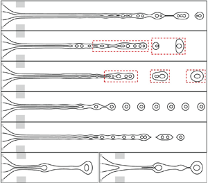
Figure 7. (a) Four typical response modes of jet breakup for a strong-coupled jet at $r_Q=0.5$, where $Re=32.7$ and $r_{Q1}+r_{Q2}=0.0714$. The letter symbols I, M, S and IJ stand for the irregular breakup mode, the multiple breakup mode, the synchronized breakup mode and the intermittent jet mode, respectively. The dashed box contains the droplets generated in one period of $1/f$. (b) Phase diagram of the response modes as the values of $f$ and $A$ vary. The dashed lines denote the boundaries of different modes roughly.

The response modes of coaxial jet breakup under different $f$ and $A$ are much more complex for a weak-coupled jet than for a strong-coupled jet, since the inner and outer jets breakup asynchronously. Figure 8(a) shows the typical response modes of jet breakup for a weak-coupled jet at $r_Q=0.1$, and the corresponding phase diagram for different response modes is given in figure 8(b). The first response mode is the ‘I-I’ mode, where both the inner and outer jets breakup in a rather irregular manner, resulting in multiple core droplets inside a shell. It is notable that the core droplets tend to merge together due to the interplay of the diffuse interface in numerical simulations. However, this merging behaviour does not prevent us from counting the number of cores inside a compound droplet. The second response mode is the ‘M-M’ mode, where both the inner and outer jets breakup with multiple droplets in a working period $1/f$, resulting in droplets with non-uniform size. The third response mode corresponds to the ‘M-S’ mode, where the inner jet presents the M mode while the outer jet breaks synchronously with actuation (S mode). In this mode, compound droplets with uniform size and multi-cores inside can be generated. The fourth response mode is the ‘S-S’ mode, in which both the inner and outer jets breakup synchronously with the actuation. Consequently, compound droplets with single core inside a shell can be generated periodically. The fifth response mode is the ‘S-I’ mode. In this mode, the formation of inner droplets is synchronized with actuation, resulting in droplets of uniform size. Meanwhile, the outer jet breaks in a rather random manner, producing non-uniform size compound droplets. The last response mode is the intermittent jet (‘IJ’) mode, in which the dynamic behaviours of the coaxial cone and jet are similar to the strong-coupled case. The phase diagram of different response modes for the weak-coupled jet is shown in figure 8(b). There exists a critical value of $A$ below which the jet breakup presents the I-I mode, indicating that the external actuation cannot modulate the jet breakup at very low amplitude. At a large value of $A$ and small value of $f$ (e.g. $A \ge 0.8$ and $f \le 10$), the coaxial jet presents the IJ mode. The response for the coaxial jet breakup is much more complicated at moderate $A$. As $f$ increases from very low values, the jet breakup presents the M-M mode and gradually transitions to the M-S, S-S, S-I and I-I modes. Specifically, the upper boundary for the synchronized frequency region is almost unaffected by $A$, while the lower boundary decreases with $A$ increasing, both for the inner and outer jets.

Figure 8. (a) Six typical response modes of jet breakup for a weak-coupled jet at $r_Q=0.1$, where $Re=32.7$ and $r_{Q1}+r_{Q2}=0.0714$. The letter symbols I-I, M-M, M-S, S-S, S-I and IJ stand for the inner and outer irregular breakup mode, the inner and outer multiple breakup mode, the inner multiple and outer synchronized breakup mode, the inner and outer synchronized breakup mode, the inner synchronized and outer irregular breakup mode, and the intermittent jet mode, respectively. The dashed box contains the droplets generated in one period of $1/f$. (b) Phase diagram of the response modes as the values of $f$ and $A$ vary. The dashed and dash-dotted lines denote the boundaries of different modes roughly.

4.2. Effect of actuation frequency

Figure 9(a) depicts the effect of actuation frequency $f$ on the breakup of the strong-coupled jet ($r_Q=0.5$) under constant perturbation amplitude $A=0.1$. The variation of the corresponding diameter of compound droplets $D_o$ changing with $f$ is shown in figure 9(b). As the inner and outer jets evolve synchronously and eventually breakup into single core droplets, the diameters of core droplets can be predicted approximately through volume conservation, i.e. $D_i \approx r_Q^{1/3} D_o$. For an unexcited jet with $f=0$, the breakup of the coaxial jet is rather random without periodicity, presenting the I mode, with the compound droplet sizes falling within a certain range. The average breakup frequency (also known as natural frequency, $f_n$) can be obtained by counting the number of droplets (denoted by $N$) in a long time sequence (denoted by $T$), which is $f_n=N/T$ and approximately equal to 23.5 in numerical simulations. The corresponding average droplets diameter is about 0.393. When the frequency increases to a relatively low value ($\,f=6$), the coaxial jet breakup shifts to the M mode, where droplets with multiple discrete values of diameters are generated during a working period of $1/f$. A continuous increase of $f$ leads to the S mode of jet breakup, which results in a droplet size. In this mode, the size and frequency of droplet generation can be effectively adjusted by varying $f$. Notably, the natural frequency $f_n$ falls within the frequency range of the S mode. If $f$ exceeds a critical value, the periodicity disappears, and the droplet generation becomes random again, leading to the I mode. The breakup characteristics are similar to those of an unexcited jet. Figure 9(b) also shows the variation tendency of droplet diameter $D_o$ with $f$. In the frequency range of the S mode, the generation of compound droplets is totally synchronized with actuation; thus, the conservation law of flow rate can be obtained as $(Q_1+Q_2)=4/3 {\rm \pi}(D_o/2)^3 (1/f)$. Therefore, the size of uniform droplets is related to the perturbation frequency $f$ and the dimensionless average flow rate of core and shell liquids, as given by $f=(Q_1+Q_2)/({\rm \pi} D_o^3/6)$. This suggests the scaling law of $D_o \sim f^{-1/3}$, which is confirmed by the numerical results in figure 9(b).

Figure 9. (a) Interface profiles of the coaxial jet as the perturbation frequency $f$ varies at $A=0.1$ and $r_Q=0.5$. (b) Diameters of compound droplets ($D_o$) under different $f$, where $f_n$ denotes the natural breakup frequency.

In order to better illustrate the dynamic characteristics of coaxial jet breakup, figure 10 presents the temporal evolution of the position of the outer jet interface tip (sketched in figure 9b). As the interface breaks up into droplets, the tip position goes through a sudden jump, and the new tip position indicates the jet breakup length. For the I mode at $f=0$ and 50, as shown in figure 10(a,d), the pinch-off positions of the interface are random and the jet breakup length varies within a certain range. At the M mode at $f=6$ (see figure 10b), multiple pinch-off positions exist in one working period of $1/f$. In the S mode at $f=35$, as demonstrated in figure 10(c), the pinch-off positions remain the same, and the jet breakup is periodic.

Figure 10. Temporal evolution of the outer jet tip position at (a) $f=0$, (b) $f=6$, (c) $f=35$ and (d) $f=50$, respectively. The pinch-off positions are also indicated.

Figure 11(a) demonstrates the effect of actuation frequency $f$ on the breakup of a weak-coupled jet ($r_Q=0.1$) under constant perturbation amplitude $A=0.1$. The corresponding diameters of compound droplets $D_o$ and core droplets $D_i$ are presented in figure 11(b), respectively. When the coaxial jet is unexcited at $f=0$, the inner jet experiences a much higher breakup frequency than the outer jet, resulting in the formation of multi-core compound droplets. Numerical results indicate that the natural breakup frequencies of the inner and outer jets are $f_{ni}=50.2$ and $f_{no}=17.5$ and the average diameters of the core and compound droplets are approximately 0.143 and 0.43, respectively. When the perturbation frequency is low ($\,f=8$), the breakup of the coaxial jet presents the M-M mode, where both the inner and outer jets form multiple droplets with different sizes during one working period of $1/f$ (see figure 11b). As $f$ gradually increases ($\,f=15$), the outer jet enters the S mode first, while the inner jet maintains the M mode (i.e. M-S mode). This occurs because the natural frequency of the outer jet is much lower than that of the inner jet. When the frequency increases to $f=25$, both the inner and outer jets break at the S mode with single-core droplet formation. In this S-S mode, the size of compound droplets can be adjusted by the actuation frequency. As $f$ increases further ($\,f=50$), the jet breakup transitions to the S-I mode. In this mode, the breakup of the outer jet loses its periodicity and returns to the I mode again, where the droplet size is located within some ranges. However, the size of the inner droplets remains uniform. At very high frequency ($\,f=100$), both the inner and outer jets break at the I mode (i.e. I-I), which is similar to the unexcited jet. Notably, in the synchronized region of the inner and outer jets, the droplet size follows the relationship $D_o \sim f^{1/3}$ and $D_i \sim f^{1/3}$, respectively, as shown clearly in figure 11(b).

Figure 11. (a) Interface profiles of the coaxial jet as the perturbation frequency $f$ varies at $A=0.1$ and $r_Q=0.1$. (b) Diameters of inner droplets ($D_i$, hollow symbols) and compound droplets ($D_o$, filled symbols) under different $f$, where $f_{ni}$ and $f_{no}$ denote the natural breakup frequencies of the inner and outer jet, respectively.

Figure 12 presents the temporal evolution of the interface tip positions of both the inner and outer jets. The results show that the pinch-off positions and the periodicity of the jet breakup are significantly affected by the actuation frequency $f$. For the I-I mode at $f=0$ and 100, as shown in figure 12(a,f), the pinch-off positions of the inner and outer interfaces are rather random, suggesting that the jet breakup length varies with time and there is no periodicity for jet breakup. For the M-M mode at $f=8$ (see figure 12b), multiple pinch-off positions exist for both the inner and outer jets in one working period of $1/f$. For the M-S mode at $f=15$, the outer jet has a constant pinch-off position while multiple pinch-off positions exist for the inner jet, as shown in figure 12(c). In the S-S mode at $f=35$, both the inner and outer jets have constant pinch-off positions, and the interface evolution is periodic (see figure 12d). In the S-I mode at $f=50$, the inner jet has a constant pinch-off position while random pinch-off positions exist for the outer jet, as shown in figure 12(e).

Figure 12. Temporal evolution of inner and outer jet tip positions at (a) $f=0$, (b) $f=8$, (c) $f=15$, (d) $f=35$, (e) $f=50$ and (f) $f=100$, respectively. The pinch-off positions are also indicated.

4.3. Effect of actuation amplitude

We also investigate the effect of actuation amplitude $A$ on the breakup of the coaxial liquid jet. An increase of $A$ can enhance the initial perturbations on the coaxial liquid cone and the jet downstream. As illustrated in figures 7(b) and 8(b), the variation of $A$ can lead to the transition between different response modes, and the jet even becomes unstable at a high value of $A$ and low value of $f$. In this section we focus on the effect of $A$ under moderate values of $f$, where the coaxial cone-jet structure can be maintained consistently.

Figure 13(a) shows the breakup profiles of the coaxial jet at $r_Q=0.5$, under a fixed $f=40$ with $A$ varying. When $A$ is at relatively low value (e.g. $A=0.03$), the external perturbation is too weak to influence the jet breakup, and the coaxial jet exhibits a non-uniform size distribution of droplets in the I mode. At moderate values of $A$, as the perturbation frequency $f$ falls within the synchronized breakup range, the coaxial jet can exhibit the S mode, displaying periodic behaviour and a consistent breakup length with no variation on droplet size. However, the variation of $A$ can significantly affect the breakup length of the jet. The relationship between jet breakup length $L$ and perturbation amplitude $A$ is given in figure 13(b), in which $L$ is measured as the distance between the pinch-off position to the orifice exit (see the sketch in figure 13a) and rescaled by the radius $r_j$ of the coaxial jet. This operation is for the convenience of comparing the numerical results with linear instability analysis, in which $r_j$ is chosen as the characteristic length. It is notable that the jet breakup length falls within certain ranges with its average value in the I mode, whereas it remains constant in the S mode. The jet breakup length appears to follow the law $L \sim -\ln A$, and we provide theoretical analysis on the jet breakup length in § 5.3.

Figure 13. (a) Interface profiles and (b) breakup length of the coaxial jet under different $A$ at $f=40$ and $r_Q=0.5$. The triangle denotes the theoretical variation slope of $-4.55$ that is predicted in § 5.3.

Figure 14(a) shows the breakup profiles of the coaxial jet at $r_Q=0.1$, under a varying $A$ for a fixed $f=15$. Similarly, when $A$ is relatively small (e.g. $A=0.03$), the external perturbation is too weak to have any significant effect on the coaxial jet breakup, and the jet presents the I-I mode. However, as $A$ gradually increases, the external perturbation can affect the coaxial jet breakup significantly. Specifically, the coaxial jet breakup exhibits the M-S mode for $A=0.1$ and 0.4, while the mode changes to the S-S mode as $A=1$. The breakup lengths of the inner and outer jets (denoted by $L_i$ and $L_o$, respectively) are defined as the distance between the pinch-off positions of the inner and outer jet to the orifice exit (see figure 14a), respectively, and the jet breakup lengths rescaled by $r_j$ are shown in figure 14(b). In the I-I mode, the values of $L_i$ and $L_o$ locate within a certain range due to the non-periodic breakup characteristics. Therefore, both the average length and the error bars are presented simultaneously. In the M-S mode the value of $L_i$ falls within a certain range while that of $L_o$ remains constant. In the S-S mode, both the inner and outer jet breakup lengths maintain the same value. Our analysis indicates that the relationship $L_i \sim -\ln A$ is a suitable model for the inner jet, whereas this model does not apply to the outer jet. Theoretical analysis on the jet breakup length will be given in § 5.3.

Figure 14. (a) Interface profiles and (b) breakup length of the coaxial jet under different $A$ at $f=15$ and $r_Q=0.1$. The triangles denote the theoretical variation slope of the inner and outer jet ($-5$ and $-10.42$, respectively) that are predicted in § 5.3.

4.4. Effect of liquid flow rates

The diameter and velocity of a coaxial liquid jet can be significantly affected by the flow rates of the core, shell and focusing liquids. Therefore, the liquid flow rates are supposed to affect the natural frequency and the synchronized region of the coaxial liquid jet. According to the definition of the dimensionless parameter in numerical simulations, $Re \sim U_3 \sim Q_3, r_{Q1}=Q_1/Q_3$ and $r_{Q2}=Q_2/Q_3$. Therefore, the change of focusing flow rate $Q_3$ corresponds to the variation of $Re$ under a constant value of $Re \,\cdot \, (r_{Q1}+r_{Q2})$, and the change of coaxial jet flow rates $Q_1+Q_2$ corresponds to the variation of $r_{Q1}+r_{Q2}$ under a constant value $Re$, respectively. Figure 15(a) shows the effect of focusing flow rate (non-dimensionalized by $Re$) for a strong-coupled jet at $r_Q=0.5$ and a constant perturbation amplitude of $A=0.1$, where $f_n$, $f_c$ and $f_l$ are the natural frequency, upper critical frequency and lower critical frequency of the synchronized region, respectively. It is worth noting that $f_n$ falls within a certain range due to the random breakup of the undisturbed jet, and its average value is given along with the error bars. As for the critical frequencies $f_c$ and $f_l$, error bars also exist due to the uncertainty on the determination of mode boundaries. It is clear that $f_n$, $f_c$ and $f_l$ all increase with $Re$ increasing, indicating that increasing the focusing flow rate can increase both the natural frequency and critical frequencies of the synchronized region. Figure 15(b) shows the effect of the sum flow rate of the inner and outer jet (non-dimensionalized by $r_{Q1}+r_{Q2}$) at $r_Q=0.5$ and $A=0.1$, which demonstrates that $f_n$, $f_c$ and $f_l$ all decrease as $r_{Q1}+r_{Q2}$ gradually increases. This finding suggests that increasing the coaxial jet flow rates can decrease both the natural frequency and critical frequencies of the synchronized region.

Figure 15. The natural frequency ($\,f_n$), lower critical frequency ($\,f_l$) and upper critical frequency ($\,f_c$) for a strong-coupled coaxial jet at $r_Q=0.5$ under constant perturbation amplitude of $A=0.1$ as the values of (a) $Re$ varies at fixed $Re \,\cdot \, (r_{Q1}+r_{Q2})=2.336$ and (b) $r_{Q1}+r_{Q2}$ varies at fixed $Re=32.7$. The natural frequency ($\,f_{no}$), lower critical frequency ($\,f_{lo}$) and upper critical frequency ($\,f_{co}$) of the outer jet and those of the inner jet (denoted by $f_{ni}$, $f_{li}$ and $f_{ci}$, respectively) for a weak-coupled coaxial jet at $r_Q=0.1$ under constant perturbation amplitude of $A=0.1$ as the values of (c) $Re$ varies at fixed $Re \,\cdot \, (r_{Q1}+r_{Q2})=2.336$ and (d) $r_{Q1}+r_{Q2}$ varies at fixed $Re=32.7$. The symbols denote the numerical results and the lines denote the theoretical predictions of scaling analysis in § 5.2.

The breakup behaviours of the weak-coupled jet are more complex due to the independent breakup of the inner and outer jets. Figure 15(c,d) shows that the natural frequency of the inner jet ($\,f_{ni}$) is significantly greater than that of the outer jet ($\,f_{no}$). In addition, the upper and lower critical frequencies of the inner jet ($\,f_{ci}$ and $\,f_{li}$, respectively) are also much larger than those of the outer jet ($\,f_{co}$ and $f_{lo}$, respectively). It is also observed that the synchronized frequency range of the inner jet is much wider than that of the outer jet. Similar to the situation of the strong-coupled jet, an increase of $Re$ or a decrease of $r_{Q1}+r_{Q2}$ can lead to the increase of natural frequency and critical frequency of both the inner and outer jets, as shown in figure 15(c,d), respectively. In § 5 we further provide theoretical predictions for the natural breakup frequency and the upper critical frequency based on the instability analysis of simplified single jet models for coaxial jets under strong and weak coupling conditions.

The effect of relative flow rate between the inner and outer jets on coaxial jet breakup is also investigated. Figure 16(a) shows the breakup profiles of the coaxial liquid jet as $r_Q$ varies under constant values of $f=30$ and $A=0.1$, where the liquid flow rates are constant at $Re=32.7$ and $r_{Q1}+r_{Q2}=0.0714$. It is observed that in a wide range of $r_Q$ ($r_Q=0.1$, 0.35 and 0.6), the inner and outer jets breakup synchronously with external perturbations under the S-S mode, resulting in uniform compound droplets with a single core inside. By varying $r_Q$, the relative size between the core and shell droplets can be well controlled, which has practical significance in real applications. However, at a very low value of $r_Q$ ($r_Q=0.05$), the inner jet loses its periodicity and the breakup of the coaxial jet presents the M-S mode, showing that the generation of core droplets cannot be controlled precisely. The reason for the aperiodicity on inner droplet formation can be explained qualitatively as: the inner jet diameter is very small at a low value of $r_Q$; therefore, the natural frequency and the frequency range of the synchronized region differs significantly between the inner and outer jets. As the value of $r_Q$ gradually decreases, the natural frequency of the inner jet ($\,f_{ni}$) increases, and the lower critical frequency of the inner jet ($\,f_{li}$) increases correspondingly. As $f_{li}$ becomes larger than the upper critical frequency of the outer jet ($\,f_{co}$), the frequency range for the S-S mode vanishes, thus, the inner jet presents the M mode while the outer jet maintains the S mode. Figure 16(b) presents the diameters of both the inner and outer droplets as $r_Q$ varies, showing that the outer droplets diameter $D_o$ keeps almost unchanged while the inner droplet diameter $D_i$ decreases with the decrease of $r_Q$. Specifically, inner droplets with multiple diameters are formed at the M-S mode when $r_Q=0.05$. In the synchronized region the outer and inner droplet diameters can be predicted theoretically by the dimensionless flow rates and frequency, i.e. $D_o=(6(Q_1+Q_2)/{\rm \pi} f)^{1/3}$ and $D_i=r_Q^{1/3}D_o$, respectively. Therefore, the outer droplet diameter $D_o$ keeps unchanged at fixed $f$, which is calculated as $D_o=0.36$ for the cases considered in figure 16(a). The theoretical prediction agrees well with the numerical results.

Figure 16. (a) Profiles of a coaxial jet at different $r_Q$ under constant values of $f=30$ and $A=0.1$. (b) Diameters of inner and outer droplets as $r_Q$ changes.

5. Theoretical analysis

5.1. Linear instability

In order to give the theoretical analysis on the breakup characteristics of coaxial liquid jets, we carry out a temporal instability analysis considering the perturbation growth on the jet interface. We mainly focus on the locally convective instability of the liquid jets, where the perturbation only propagates downstream the jet that induces the generation of droplets (Lin 2003; Eggers & Villermaux 2008). Such an assumption is appropriate for the coaxial liquid jets with parallel flow characteristics downstream of the orifice. For convenience, we can simplify the coaxial jet to a single jet model at different interface coupling situations, as illustrated in figure 17. On one hand, at relatively large $r_Q$ that corresponds to the jet diameter ratio $\kappa \rightarrow 1$, the coupling of interfaces is strong and the coaxial jet can be simplified as a single liquid jet where the shell phase is neglected, and the equivalent interfacial tension equals the sum of the inner and outer jets, as shown in figure 17(b). Therefore, the diameter and the surface tension coefficient of the simplified jet is $\kappa d_j$ and $2\sigma$, respectively, where $d_j$ is the diameter of the coaxial jet. On the other hand, at relatively low $r_Q$ ($\kappa \rightarrow 0$), the coupling effect between the double interfaces is very weak, thus, the coaxial jet can be decoupled as two single jets, as illustrated in figure 17(c). The diameters of the inner and outer jets are $\kappa d_j$ and $d_j$, respectively. In our theoretical model we assume equal velocities of the inner jet, the outer jet and the surrounding flow, which has been proved reasonable for the all-liquid system in previous studies (Gañán-Calvo & Riesco-Chueca 2006; Gañán-Calvo et al. 2007). The simplified single jet models for weak- and strong-coupled coaxial jets enable us to study behaviours of coaxial jet breakup at extreme conditions.

Figure 17. (a) Theoretical model for the coaxial liquid jet, where the diameter ratio between the inner and outer jet is denoted by $\kappa$. (b) Simplified single jet model as $\kappa \rightarrow 1$, corresponding to the situation of large $r_Q$. (c) Simplified single jet model as $\kappa \rightarrow 0$, corresponding to the situation of small $r_Q$.

For the linear instability analysis, we choose the jet radius $d_j/2$ and the average velocity $U_j$ as the characteristic length and velocity, respectively. The dimensionless parameters for the single jet models in theoretical analysis are the Weber number $We_t=\rho _jU_j^2d_j/2\sigma$, the Reynolds number $Re_t=\rho _jU_jd_j/2\mu _j$, the density ratio $S=\rho _e/\rho _j$ and the viscosity ratio $N=\mu _e/\mu _j$, where $\rho _j$ and $\mu _j$ are the density and viscosity of the liquid jet while $\rho _e$ and $\mu _e$ are those of the surrounding environment, respectively. The theoretical model is solved through the normal mode method, in which the terms such as flow velocity, pressure and interface position in Navier–Stokes equations are decomposed to basic quantities and small axisymmetric perturbations with the Fourier form $\sim {\rm e}^{\mathrm {i}(k z-\omega t)}$. It is notable that $k$ is the dimensionless wavenumber, $\omega =\omega _r+\mathrm {i} \omega _i$ is the dimensionless complex frequency, where $\omega _i$ and $-\omega _r$ denote the growth rate and temporal frequency of perturbations, respectively. The perturbations with $\omega _i>0$ are temporally unstable while those with $\omega _i<0$ are stable invariably. In our work, the perturbation frequency $-\omega _r$ will be utilized to predict the natural and critical frequencies of coaxial jet breakup under different coupling situations (see § 5.2), and the growth rate $\omega _i$ will be used to analyse the jet breakup length, as shown in § 5.3. The governing equations and boundary conditions for the single jet model are similar to those in Si et al. (2009) and are simply shown in Appendix A. Specifically, for the model at $\kappa \rightarrow 1$ shown in figure 17(b), we have $\rho _j=\rho _e=\rho _1$ and $\mu _j=\mu _e=\mu _1$. For the models at $\kappa \rightarrow 0$ shown in figure 17(c), the inner jet model corresponds to $\rho _j=\rho _1$, $\rho _e=\rho _2$, $\mu _j=\mu _1$ and $\mu _e=\mu _2$, while the outer jet model corresponds to $\rho _j=\rho _2$, $\rho _e=\rho _1$, $\mu _j=\mu _2$ and $\mu _e=\mu _1$.

5.2. Prediction of natural and critical frequencies

Based on the results obtained from the linear instability analysis, we can give the scaling analysis on the natural frequency and the upper critical frequency of the synchronized breakup region. For a single liquid jet with average velocity $U_j$ and diameter $d_j$, the natural breakup frequency $f_n$ is directly related to the jet oscillation frequency $-\omega _{rm}$ that corresponds to the maximum growth rate of the perturbation wave (whose wavenumber is denoted as $k_m$), with the quantitative estimation of

(5.1)\begin{equation} f_n=\frac{-\omega_{rm} U_j}{{\rm \pi} d_j}. \end{equation}

In the flow focusing process, $d_j$ and $U_j$ can be estimated by the simple scaling law of $d_j=d \,\cdot \, [Q_j/(Q_j+Q_e)]^{1/2}$ and $U_j=4Q_j/{\rm \pi} d_j^2$, respectively. Here, $Q_j$ and $Q_e$ denote the flow rates of the liquid jet and co-flowing liquid and $d$ is the orifice diameter. Therefore, the natural frequency can be expressed as

(5.2)\begin{equation} f_n=\frac{4}{{\rm \pi}^2 d^3}\,\cdot \, \frac{(-\omega_{rm}) (Q_j+Q_e)^{3/2}}{Q_j^{{1}/{2}}}. \end{equation}

Similarly, the upper critical frequency below which the external perturbation can modulate the jet breakup can be expressed as

(5.3)\begin{equation} f_c=\frac{4}{{\rm \pi}^2 d^3}\,\cdot \, \frac{(-\omega_{rc}) (Q_j+Q_e)^{3/2}}{Q_j^{{1}/{2}}}, \end{equation}

where $-\omega _{rc}$ is critical frequency that corresponds to the cutoff wavenumber ($k_c$) of the perturbation growth rate. When the wavenumber is larger than $k_c$, the perturbation growth rate becomes smaller than zero, and the liquid jet is invariably stable.

In this study, as we have simplified the coaxial jet to single jet models under different coupling situations, the natural and upper critical frequencies can be predicted similarly. For a strong-coupled jet, the coaxial liquid can be reduced to the single jet model in figure 17(b), and the natural and upper critical frequencies are expressed as

(5.4) \begin{equation} \left.\begin{array}{c@{}} \displaystyle f_n=\dfrac{4}{{\rm \pi}^2d^3}\,\cdot \, \dfrac{(-\omega'_{rm}) (Q_1+Q_2+Q_3)^{3/2}}{(Q_1+Q_2)^{1/2}},\\ \displaystyle f_c=\dfrac{4}{{\rm \pi}^2d^3}\,\cdot \, \dfrac{(-\omega'_{rc}) (Q_1+Q_2+Q_3)^{3/2}}{(Q_1+Q_2)^{1/2}}, \end{array}\right\} \end{equation}

where $-\omega '_{rm}$ is the frequency of the perturbation wave with the maximum growth rate, and $-\omega '_{rc}$ is the frequency that corresponds to the cutoff wavenumber, as sketched in figure 18(a,b).

Figure 18. Perturbation growth rate $\omega _i$ and frequency $-\omega _r$ versus wavenumber $k$ for different single jet models given in figure 17. (a) Variation of $Re$ under fixed $Re \,\cdot \, (r_{Q1}+r_{Q2})$ for the strong-coupled jet at $r_Q=0.5$, corresponding to $\kappa =0.71$. (b) Variation of $r_{Q1}+r_{Q2}$ under fixed $Re$ for the strong-coupled jet at $r_Q=0.5$. (c) Variation of $Re$ under fixed $Re \,\cdot \, (r_{Q1}+r_{Q2})$ for the outer jet of the weak-coupled jet at $r_Q=0.1$, corresponding to $\kappa =0.33$. (d) Variation of $r_{Q1}+r_{Q2}$ under fixed $Re$ for the outer jet of the weak-coupled jet at $r_Q=0.1$. (e) Variation of $Re$ under fixed $Re \,\cdot \, (r_{Q1}+r_{Q2})$ for the inner jet of the weak-coupled jet at $r_Q=0.1$. (f) Variation of $r_{Q1}+r_{Q2}$ under fixed $Re$ for the inner jet of the weak-coupled jet at $r_Q=0.1$.

As for a weak-coupled coaxial liquid jet that can be viewed as two single jets, as shown in figure 17(c), the natural and upper critical frequencies of the outer jet and inner jet can be expressed as

(5.5)$$\begin{gather} \left.\begin{array}{c@{}} \displaystyle f_{no}=\dfrac{4}{{\rm \pi}^2d^3}\,\cdot \, \dfrac{(-\omega''_{rm})(Q_1+Q_2+Q_3)^{3/2}}{(Q_1+Q_2)^{1/2}},\\ \displaystyle f_{co}=\dfrac{4}{{\rm \pi}^2d^3}\,\cdot \, \dfrac{(-\omega''_{rc}) (Q_1+Q_2+Q_3)^{3/2}}{(Q_1+Q_2)^{1/2}}, \end{array}\right\} \end{gather}$$

(5.6)$$\begin{gather}\left.\begin{array}{c@{}} \displaystyle f_{ni}=\dfrac{4}{{\rm \pi}^2d^3}\,\cdot \, \dfrac{(-\omega'''_{rm}) (Q_1+Q_2+Q_3)^{3/2}}{(Q_1+Q_2)^{1/2}},\\ \displaystyle f_{ci}=\dfrac{4}{{\rm \pi}^2d^3}\,\cdot \, \dfrac{(-\omega'''_{rc}) (Q_1+Q_2+Q_3)^{3/2}}{(Q_1+Q_2)^{1/2}}, \end{array}\right\} \end{gather}$$

where $-\omega ''_{rm}$ and $-\omega ''_{rc}$ are the oscillation frequencies that correspond to the perturbation wave with the maximum growth rate and the cutoff wavenumber of the outer jet model (see figure 18c,d), while $-\omega '''_{rm}$ and $-\omega '''_{rc}$ are the oscillation frequencies of the perturbation waves with the maximum growth rate and the cutoff wavenumber of the inner jet model, respectively (see figure 18e,f).

According to our definition of parameters, the dimensionless frequency can be written in the form of $Re$, $r_{Q1}$ and $r_{Q2}$, i.e.

(5.7a,b)\begin{equation} f_n=C \,\cdot \, \frac{(-\omega'_{rm}) (r_{Q1}+r_{Q2}+1)^{3/2}}{(r_{Q1}+r_{Q2})^{1/2}},\quad f_c=C \,\cdot \, \frac{(-\omega'_{rc}) (r_{Q1}+r_{Q2}+1)^{3/2}}{(r_{Q1}+r_{Q2})^{1/2}}, \end{equation}

for the strong-coupled jet, and

(5.8a,b)$$\begin{gather} f_{no}=C \,\cdot \, \frac{(-\omega''_{rm}) (r_{Q1}+r_{Q2}+1)^{3/2}}{(r_{Q1}+r_{Q2})^{1/2}},\quad f_{co}=C \,\cdot \, \frac{(-\omega''_{rc}) (r_{Q1}+r_{Q2}+1)^{3/2}}{(r_{Q1}+r_{Q2})^{1/2}}, \end{gather}$$

(5.9a,b)$$\begin{gather}f_{ni}=C \,\cdot \, \frac{(-\omega'''_{rm}) (r_{Q1}+r_{Q2}+1)^{3/2}}{(r_{Q1}+r_{Q2})^{1/2}},\quad f_{ci}=C \,\cdot \, \frac{(-\omega'''_{rc}) (r_{Q1}+r_{Q2}+1)^{3/2}}{(r_{Q1}+r_{Q2})^{1/2}}, \end{gather}$$

for the outer and inner jet of the weak-coupled jet, respectively. In these equations, $C$ is a constant with its value decided by the geometrical parameters $D_2$ and $d$, which equals a specific value of 8.5 in our simulations.

It is notable that (5.7), (5.8) and (5.9) do not contain $Re$ explicitly. However, the variation of $Re$ in figure 15(a,c) also leads to the corresponding change of $r_{Q1}+r_{Q2}$, indicating that the single variation of focusing flow rate can change the natural breakup frequency and upper critical frequency of the synchronized region.

The oscillation frequencies that correspond to the maximum perturbation growth rate and the cutoff wavenumber in (5.7), (5.8) and (5.9) can be determined by linear instability analysis on the simplified single jet models. Figure 18(a,b) shows the perturbation growth rate curves and the oscillation frequency curves of the simplified single jet for the strong-coupled jet at $r_Q=0.5$ (corresponding to $\kappa =0.71$), considering (a) the variation of $Re$ under fixed $Re \,\cdot \, (r_{Q1}+r_{Q2})$ and (b) the variation of $r_{Q1}+r_{Q2}$ under fixed $Re$, respectively. It is notable that the variation of $Re$ or $r_{Q1}+r_{Q2}$ affects the growth rate curves significantly but hardly changes the oscillation frequency curves. For each curve, we can determine the values of the most unstable wavenumber $k'_m$ and the cutoff wavenumber $k'_c$ and then obtain the values of $-\omega '_{rm}$ and $-\omega '_{rc}$, respectively. It is notable that for the cases considered here, the value of the dimensionless frequency is equal to that of the wavenumber invariably (i.e. $-\omega '_{rm}=k'_m$ and $-\omega '_{rc}=k'_c$), indicating that the perturbation propagates with a dimensionless phase velocity of $-\omega '_r/k=1$. Therefore, if one stands on the axial local framework along with the liquid jet, the interface disturbance only grows temporally and hardly propagates upstream or downstream of the jet, which is similar to the standard temporal stability analysis of the capillary jet (Lin 2003; Eggers & Villermaux 2008). The results indicate that the variation of $Re$ or $r_{Q1}+r_{Q2}$ mainly affects the perturbation growth rate $\omega _i$ but only has a tiny effect on the wavenumber corresponding to the maximum growth rate and the cutoff wavenumber. In all cases examined in figure 18(a,b), $k'_c$ is at a constant value of 1.41 and $k'_m$ only varies slightly within $0.82 \pm 0.01$. As for the weak-coupled jet at $r_Q=0.1$ (corresponding to $\kappa =0.33$), the outer and inner jets are analysed independently. For the outer jet, the perturbation growth rate curves and the oscillation frequency curves as $Re$ varies under fixed $Re \,\cdot \, (r_{Q1}+r_{Q2})$ and those as $r_{Q1}+r_{Q2}$ varies under fixed $Re$ are given in figure 18(c,d), respectively. Similarly, the variation of $Re$ or $r_{Q1}+r_{Q2}$ only has a tiny effect on the wavenumber corresponding to the maximum growth rate and the cutoff wavenumber. Within the parameter range we consider, $-\omega ''_{rm}=k''_m$ and $-\omega ''_{rc}=k''_c$, with $k''_c=1$ and $k''_m=0.49 \pm 0.01$. For the inner jet, the perturbation growth rate curves and the oscillation frequency curves as $Re$ varies under fixed $Re \,\cdot \, (r_{Q1}+r_{Q2})$ and those as $r_{Q1}+r_{Q2}$ varies under fixed $Re$ are given in figure 18(e,f), respectively. Similarly, the cutoff wavenumber and the wavenumber corresponding to the maximum growth rate hardly change, in which $-\omega '''_{rm}=k'''_m=1.58 \pm 0.01$ and $-\omega ''_{rc}=k'''_c=3$. With the wavenumber being determined, the theoretical predictions of $f_n$ and $f_c$ for the strong-coupled jet and $f_{no}, f_{co}, f_{ni}$ and $f_{ci}$ for the weak-coupled jet can be obtained according to (5.7)–(5.9). The theoretical results are depicted as lines in figure 15, showing a good agreement with the numerical results.

5.3. Predictions of jet breakup length

For a liquid jet with radius $r_j$, the perturbation on the interface develops with growth rate $\omega _i$ and initial magnitude $\eta _0$. Under the linear instability frame, they follow the relationship

(5.10)\begin{equation} r_j=\eta_0 \,\mathrm{e}^{\omega_i t_b}, \end{equation}

where $t_b$ is the jet breakup time, and it can be expressed as

(5.11)\begin{equation} t_b=\frac{1}{\omega_i} \ln\frac{r_j}{\eta_0}. \end{equation}

The jet breakup length $L_j$ can be calculated through multiplying the jet velocity $U_j$ with $t_b$, i.e.

(5.12)\begin{equation} L_j=\frac{U_j}{\omega_i} \ln \frac{r_j}{\eta_0}. \end{equation}

Previous research by Moallemi et al. (2016) has established that the initial interface perturbation of a single jet is related to the flow rate perturbation $A_j$ of the liquid jet through a linear relationship, i.e. $\eta _0 \sim A_j$. Moreover, the flow rate perturbation $A_j$ has been found to be almost in direct proportion to that of the capillary tube $A$, i.e. $A_j \sim A$, as shown in figures 3(a) and 5(a), respectively. Therefore, the relationship between $L_j$ and $A$ can be expressed as

(5.13)\begin{equation} L_j \sim \frac{U_j}{\omega_i} \ln \frac{r_j}{A}. \end{equation}

It is notable that in linear instability analysis, $r_j$ and $U_j$ are chosen as the characteristic length and velocity, respectively. Therefore, (5.13) gives the relationship $L_j \sim -\ln A$, and the slope can be decided by the value of $-1/\omega _i$.

For the coaxial liquid jet, as we have simplified the coaxial jet to a single jet at different coupling situations, the jet breakup length can be predicted similarly. For the strong-coupled jet ($r_Q=0.5$) in figure 13, the jet breakup length $L$ rescaled by $r_j$ obeys the law of $L/r_j \sim -\ln A$. To estimate the slope of the curve, the growth rate $\omega _i$ at the corresponding actuation frequency ($\,f=40$) can be obtained from the growth rate curve, which corresponds to the curve $Re=32.7$ in figure 18(a). The frequency $f=40$ corresponds to a wavenumber $k=1.19$ at which the growth rate $\omega _i \approx 0.22$. Therefore, the estimated slope is about $-$4.55. Figure 13(b) also gives the slope predicted by the theory, as shown by the triangle, which agrees well with the numerical results.

The breakup length of the inner and outer jets for the weak-coupled coaxial jet at $r_Q=0.1$ can be analysed independently. Based on the simplified single jet models, the breakup length of the inner and outer jets can be expressed as

(5.14)\begin{equation} L_i \sim \frac{U_j}{\omega_i} \ln \frac{r_j}{A} \end{equation}

and

(5.15)\begin{equation} L_o \sim \frac{U_j}{\omega_i} \ln \frac{r_j}{A}. \end{equation}

Choosing $r_j$ and $U_j$ as the characteristic scales, (5.14) and (5.15) are simplified as $L_i \sim -\ln A$ and $L_o \sim -\ln A$. For the numerical results in figure 14, the slopes on the variation of $L_i/r_j$ and $L_o/r_j$ with $A$ are decided by the growth rates of the inner and outer jet, respectively. According to figure 18(c,e), the growth rate $\omega _i$ at $f=15$ can be obtained from the curve that corresponds to the situation $Re=32.7$. The frequency $f=15$ corresponds to a wavenumber $k=0.45$, and the growth rates of the inner and outer jets are $\omega _i \approx 0.2$ and 0.096, respectively. Therefore, the slope $-1/\omega _i$ of the inner and outer jets can be estimated as $-$5 and $-$10.42, respectively. Figure 14(b) also gives the theoretical slope for the inner and outer jets, respectively, as shown by the triangles. It is clear that the theoretical prediction of the inner jet agrees well with the numerical results, while that of the outer jet diverges significantly from the numerical results. The results suggest that the breakup of the inner droplet brings in additional perturbation and, thus, has a huge influence on the breakup length of the outer jet, even in the weak-coupled situation.

6. Controllable formation of multi-core droplets

As we have found in figure 11, compound droplets with a single core inside a shell can be produced precisely within the frequency range in which the inner and outer jets both exhibit synchronized breakup with external actuation. In this section we extend our study to investigate the formation of compound droplets with a controlled number of cores. In previous experiments of Bocanegra et al. (2005), they successfully controlled the core numbers to seven through adding a pulse with a large amplitude every seven periods. Following their strategy, we bring in the pulse on the flow rate actuation and examine the production of a compound droplet with controllable cores. Figure 19(a) shows the sketch of the perturbation wave with a pulse every $N$ period, and the amplitude of the pulse is denoted by $A_p$. The jet breakup profiles under $f=70$, $A=0.1$, $A_p=4A=0.4$ but different $N$ are given in figure 19(b), respectively. Our results indicate that at a relatively small $N$ (e.g. $N=2$, 4, 6 and 8), uniform compound droplets with $N$ cores inside can be successfully produced, which is similar to the approach adopted by Bocanegra et al. (2005). The generation of compound droplets obeys a working frequency of $f/N$. Therefore, the size of compound droplets increases as $N$ increases. However, at relatively large $N$ (e.g. $N=10$), the compound droplets cannot maintain uniformity in size. Instead, the production of compound droplets follows the multiple breakup (M) mode, where two droplets are generated in a working frequency $f/N$. The mechanism for the occurrence of the M mode as $N$ gradually increases can be explained through comparing the working frequency $f/N$ with the synchronized frequency region of the outer jet. For the liquid flow rates we consider here ($Re=32.7$, $r_{Q1}+r_{Q2}=0.0714$ and $r_Q=0.1$), figure 15(c,d) indicates the synchronized frequency region of the outer jet, which is $f=9\unicode{x2013} 37$ under constant perturbation amplitude $A=0.1$. When the pulse is added on the flow, the working frequency corresponds to $f/N=35$, 17.5, 11.7 and 8.8 as $N=2$, 4, 6 and 8, respectively. As the values of working frequency are almost completely located within the synchronized frequency range of the outer jet, the outer jet is able to present a synchronized breakup manner with uniform compound droplets generated. However, as $N$ increases to 10, the working frequency corresponds to $f/N=7$, which is obviously lower than the critical frequency for the synchronized breakup of the outer jet; thus, the outer jet presents the M mode with multiple droplets generated in one period. Overall, we can conclude that the method of adding pulse is most suitable for the situation when the frequency $f/N$ locates within the synchronized frequency region of the outer jet.

Figure 19. (a) Sketch of the perturbation wave with pulse every $N$ periods. (b) Breakup of the weak-coupled coaxial jet ($r_Q=0.1$) under different $N$ at $f=70$, $A=0.1$ and $A_p=4A$.

7. Conclusions

We study the interfacial flow and instability of a coaxial liquid jet in CFF upon actuation through direct numerical simulations by solving the Navier–Stokes equations coupled with a diffuse interface method. Synchronized actuations on the flow rates of core and shell liquids are applied to modulate the flow, and the effects of perturbation frequency, amplitude and liquid flow rates on the evolution of coaxial liquid cones and jets are investigated. The coaxial cone can serve as a reservoir that modulates the external perturbation of the jet. An increase of perturbation amplitude and a decrease of perturbation frequency can increase the local perturbation amplitude of the jet. The coaxial cone can also destabilize at a large perturbation amplitude and small frequency, recoiling upstream of the orifice with intermittent jet behaviour. The relative flow rate between the inner jet and the coaxial jet (denoted by $r_Q$) plays a significant role on the coupling manner of double interfaces, which has a huge impact on the response modes of jet breakup under external actuation. The effects of perturbation frequency, amplitude and flow rates of core, shell and focusing liquid on the jet breakup modes are studied. It is found that the breakup modes of a weak-coupled jet at small $r_Q$ are much more complicated than those of a strong-coupled jet at large $r_Q$. Within some frequency range, the breakup of inner and outer jets can be synchronized with external actuation, producing single-encapsulated compound droplets with uniform size. The size of compound droplets can be adjusted by the variation of frequency. The natural frequency of jet breakup locates within the frequency range of the synchronized breakup region. The coaxial jets under weak and strong coupling behaviours are simplified to single jet models, respectively. The scaling analysis and linear instability analysis on these single jet models are carried out, which predict the variation tendency of jet breakup length with actuation amplitude and the natural frequency and the critical frequency for the synchronized breakup region. Furthermore, a strong pulse is added on the perturbation waveform, and the number of cores inside the compound droplets can be precisely controlled through changing the period of the pulse. The critical condition for the feasibility of this strategy is also indicated through comparing the working frequency with the lower critical frequency of the synchronized region. Overall, this numerical investigation can provide guidance for experimental study on active CFF, which is supposed to contribute to the on-demand compound droplets generation in many practical applications.