Baroclinic critical layer in a viscous stratified boundary layer flow on an undulated tilted surface

Abstract

The present paper investigates theoretically and experimentally the boundary layer generated by a stably stratified fluid flowing horizontally along a surface tilted in the transverse direction and deformed by sinusoidal undulations with crests perpendicular to the flow direction. In the absence of undulations, a weak transverse velocity proportional to the normal velocity is created such that the flow remains purely horizontal. In the presence of undulations of amplitude $h$, a stronger transverse flow is generated that exhibits a singular behaviour at the critical altitude where the frequency of the perturbation matches the buoyancy frequency of the fluid. This baroclinic critical layer was previously analysed by Passaggia et al. (J. Fluid Mech., vol. 751, 2014, pp. 663–684) for a boundary layer flow with a small sliding velocity on the surface. Here, the no-slip boundary condition of the experimental flow is applied. For this purpose, we solve the viscous sub-layer to obtain a complete theoretical model for the solution in the critical layer without any adjusting parameter. The theoretical predictions for the transverse velocity are compared with experimental measurements, and a good quantitative agreement is demonstrated. Compared with the sliding case, the no-slip boundary condition on the surface reduces the amplitude of the critical layer solution by a factor $Re^{-1/3}$, where the Reynolds number Re is defined using the velocity at infinity and the thickness of the boundary layer. As a consequence, the transverse velocity has a maximum in the critical layer of order $h$, but it still induces a shear rate of order $h\,Re^{1/3}$.

1. Introduction

Boundary flows of stratified fluids are often studied in an oceanographic context. Indeed, they have a strong influence on sediment dispersion (Rebesco et al. 2014) but also on the global ocean dynamics. For instance, they affect the global overturning circulation of oceans (Kuhlbrodt et al. 2007) via the currents appearing on Antarctic coastal slopes (Baines & Condie 1998; Thompson et al. 2018). This last phenomenon has motivated numerous gravity current studies, which are also relevant for atmospheric applications such as katabatic winds (Baines 2001; Monti et al. 2002; Shapiro, Huthnance & Ivanov 2003; Baines 2005). Boundary layers are places of intense dissipation (Sen, Scott & Arbic 2008; Beckebanze et al. 2018; Davis et al. 2019), but also regions where internal gravity waves (Garrett & Kunze 2007) and intense mean flow (Le Dizès 2020) are generated.

For large Reynolds numbers, the Blasius boundary layer flow that develop on a plane surface is known to be unstable (Schlichting 1979). This two-dimensional viscous instability does not disappear in the presence of stratification (Wu & Zhang 2008a; Chen, Bai & Le Dizès 2016). However, another instability, of inviscid nature, appears as soon as the stratification and the shearing directions are no longer aligned (Candelier, Le Dizès & Millet 2012; Chen et al. 2016). This instability, which is characterised by an internal gravity wave emission, has been observed in other contexts (Lindzen & Barker 1985; Le Dizès & Billant 2009). In the present experimental study, the Reynolds number will be too small for any of these instabilities to be present.

Stratified boundary layers are also particularly sensitive to topography. Wu & Zhang (2008b) showed for example that an obstacle can induce a coupling between internal waves and viscous instability modes of the boundary layer. Besides, the presence of an inclination angle between the stratification direction and the boundary has strong consequences for the flow (Garrett, MacCready & Rhines 1993), influencing transport and mixing, as observed by Phillips, Shyu & Salmun (1986) and also reported by Baines & Condie (1998). Recently, Puthan et al. (2019) numerically demonstrated that a density perturbation in a stratified fluid above a surface inclined at an angle $\alpha$ can lead to the generation of a mean oscillating flow along the slope at the frequency $N \sin \alpha$, where N is the buoyancy frequency. Furthermore, in the case of a corrugated surface, inclination enables the flow to avoid surface roughness without vertical displacement (inhibited by stratification) by going around the obstacle horizontally. The two swerve regimes (going around with a pure horizontal motion, or above) have been discussed by MacCready & Pawlak (2001).

The precise structure of a stratified boundary layer developing above an undulated inclined wall has been addressed by Passaggia, Meunier & Le Dizès (2014) using numerical simulations. Considering small sinusoidal undulations of a surface, with crest line perpendicular to the flow direction and slip boundary conditions, they predicted the generation of a strong transverse flow at a specific location in the boundary layer. They further showed that this flow is associated with a resonance mechanism between the Brunt–Väisälä frequency and the forcing of the undulations at a critical point singularity of the inviscid equations.

Such a baroclinic critical layer has been observed in other contexts. Boulanger, Meunier & Le Dizès (2007) showed that it was excited when the axis of a vortex was tilted with respect to the direction of the stratification. They demonstrated that a strong axial flow, localised in the baroclinic critical layer, was created and could be destabilised (Boulanger, Meunier & Le Dizès 2008). Wang & Balmforth (2020, 2021) argued that similar critical layers could be responsible for the complex nonlinear dynamics observed in accretion disks (Marcus et al. 2013).

The main objective of the present work is to observe experimentally the baroclinic critical layer in a boundary layer flow and to compare the experimental data with the critical layer predictions. For this purpose, we will also need to extend the theoretical analysis of Passaggia et al. (2014) to account for the no-slip boundary condition on the undulated surface.

The paper is organised as follows. In § 2, experimental details are given: the set-up and visualisation techniques are first described and the plate design explained. The main parameters of the study and their chosen definition are presented. Section 3 focuses on the derivation of the stratified boundary layer flow on a flat inclined wall, and first comparisons with experimental measurements. This solution constitutes the base flow that is perturbed in § 4 by small undulations of the plate. The extension of the Passaggia et al. (2014) analysis is carried out here. In particular, we solve the viscous sub-layer needed to apply the no-slip boundary condition. A parameterless expression for the transverse velocity in the baroclinic critical layer is obtained and compared with experimental measurements. A good qualitative and quantitative agreement is demonstrated. Section 5 summarises the main results and briefly discusses an application to a real atmospheric flow.

2. A stratified boundary layer experiment

A brief description of the experiment is provided in this section. More details on the facility, stratification method and visualisation subtleties can be found in the PhD thesis of Christin (2021).

2.1. Facility

The experimental set-up, sketched in figure 1(a), consists of a poly-methyl methacrylate (PMMA) tank 4 m long, 1 m wide and 1 m deep, filled with salty water up to a height $H\sim 85$ cm. A trolley is mounted on rails and moved with a ball screw connected to a motor MAC800 D2 of JVL, allowing a horizontal translation of the plate along the tank. The velocity of the trolley is kept constant during each run and varies in the range $1.79 \leqslant U \leqslant 2.98\ {\rm cm}\ {\rm s}^{-1}$.

Figure 1. (a) Schematic of the experimental set-up indicating the main axes. The horizontal/vertical coordinates $(X,Y,Z)$ are rotated with an angle $\alpha$ around the $X$-axis to give the new coordinates $(x,y,z)$. The plate is in the $(x,y)$ plane such that its outgoing normal $\boldsymbol {e}_{\boldsymbol {z}}$ is tilted with an angle $\alpha$ with respect to ${\boldsymbol {e}_{\boldsymbol {Z}}}$ (i.e. with an angle ${\rm \pi} -\alpha$ with respect to $\boldsymbol {g}$). The plate is tilted around the $y$ axis by a small angle $\gamma =2^\circ$ to prevent boundary layer separation. The undulations have a wavelength $\lambda$ and an amplitude $h$. (b) Schematic of the visualisation set-up including both shadowgraph (in yellow) and particle image velocimetry (in green).

As shown in the sketch, the plate is fixed to the trolley thanks to four supporting arms. The study is done on the lower side, so that the arms do not perturb the region of interest. The plate consists of a plane entrance zone where the boundary layer can develop before reaching the undulations. This region is needed to obtain a sufficiently large boundary layer width $\delta$ in the undulation zone. The corrugated part consists in 5 undulations, of half-crest-to-crest height $h$ and wavelength $\lambda$ (wavenumber $k$), and is the zone of interest in this study. It is parametrised as $\xi (x)=h \sin {k(x-L_u)}$, for $x>L_u$, where $L_u$ is the distance between the leading edge of the plate and the beginning of the sinusoidal part. The transition between plane and undulated parts is smoothed thanks to a bending radius.

Another important element of the present work is $\alpha$, the angle made between the outward normal of the plate surface ${\boldsymbol {e}_{\boldsymbol {z}}}$ and the upward vertical $\boldsymbol {e}_{\boldsymbol {Z}}$. It generates a transverse inclination of the plate and is necessary for the critical layer to exist.

Figure 1(a) also shows a second angle, $\gamma =2^\circ$, made between the horizontal and the longitudinal direction of the plate. This very small angle is needed to relaminarise the boundary layer, as will be seen in § 2.4.

2.2. Stratification

The tank is filled with salty water with a salt concentration increasing linearly with depth. The Brunt–Väisälä frequency is then defined as

(2.1)\begin{equation} N=\displaystyle \sqrt{-\frac{g}{\rho_0}\,\frac{\partial \rho_{lin}}{\partial Z}}, \end{equation}

where $\rho _{lin}$ is the fluid density, $\rho _0$ the density at the mean plate height, $g$ the gravity and $Z$ the coordinate along the vertical.

This stratification is obtained using a technique described in the PhD thesis of Bosco (2015) and improved by Christin (2021). It consists in dividing the tank into two parts, one with pure water and the other one with uniformly mixed strongly salty water, and letting the two fluids mix through holes of diameter $0.5$ cm drilled in the separation slab. This technique is preferred to the usual ‘two tanks method’ because it requires only one tank, which is far more convenient considering the huge volume used here.

Once realised, the stratification can hold for months if the experiments performed in the tank do not generate a very violent mixing. The density profile is measured by collecting fluid samples along a tank wall in the middle of its length, every 5 cm. This is done once every day before experiments are carried out, thanks to an Anton Paar densitometer DMA 35. Between two consecutive experimental days, the profile is barely observed to change. The slope estimation induces uncertainties on $N$ of the order of 5 %.

Final experiments which lead to the results of § 4.3 are made in a stratification with constant frequency $N=0.85\pm 0.04\ {\rm rad}\ {\rm s}^{-1}$.

2.3. Measurement techniques

Two measurement techniques have been used and recorded with the same camera Sony $\alpha 7s$ taking 25 frames per second.

Firstly, the flow was qualitatively observed by a shadowgraph method (see set-up in yellow in figure 1b) which consists of observing the flow illuminated from the back, through a lens. It is based on the fact that the flow induces inhomogeneities in the density field, resulting in variations in the light refraction index which reveal the flow structure. The contrast can be adjusted by moving the camera around the focal point of the lens. On the camera is mounted a FE 2.8/50 MACRO lens, while the external lens used to focus the rays on the camera sensor is a PCX condenser lens from Edmund Optics of focal length 50 cm and diameter 25 cm.

The final results, revealing the critical layer, are obtained thanks to a particle image velocimetry (PIV) system shown in green in figure 1(b). This method requires us to seed the flow with particles (polydisperse hollow glass spheres from TSI) that are then lit by a laser sheet (Z40M18B-F-532-Ip20 from Z LASER of 532 nm wavelength), and to treat the images thanks to software (DPIVSoft on MATLAB) to deduce the velocity field. This experimental technique is quantitative but complex in its execution, for its purely experimental part as well as its data post-processing.

The seeding particles have been carefully chosen to be good tracers of the flow, meaning that their density (between 1.05 and $1.15\ {\rm g}\ {\rm cm}^{-3}$) is close to that of the ambient fluid ($\rho \in [1;1.12] {\rm g}\ {\rm cm}^{-3}$) to avoid inertial effects, and their diameter, between 8 and $12\ \mathrm {\mu }{\rm m}$, is lower than the size of the smallest structure of interest in the flow. In order to have a precise flow field, a macro lens of focal length 2.8 mm and diameter 90 mm is mounted on the camera. The laser sheet extends in the cross-flow direction, placed such that it cuts the plate on its centre part along the $\boldsymbol {e}_{\boldsymbol {y}}$ axis. Furthermore, it makes an angle $\beta =20.0\pm 0.3^\circ$ with the longitudinal axis of the plate $\boldsymbol {e}_{\boldsymbol {x}}$, shown in the bottom sketch (entitled ‘side view’) of figure 1(b). This peculiar disposition enables a scan of the velocity in the whole boundary layer depth since the velocity field is steady. It, however, requires a complex reconstruction of the flow field in real space (see Christin 2021). As the camera axis is aligned with $\boldsymbol {e}_{\boldsymbol {z}}$ (we neglect the very small angle $\gamma$), PIV gives the $x$ and $y$ components of the velocity.

The present study needs the PIV to be accurate for small transverse displacements (of few ${\rm mm}\ {\rm s}^{-1}$) while measuring large longitudinal velocities (up to ${\sim }3\ {\rm cm}\ {\rm s}^{-1}$) close to the plate. In order to do so, for the highest considered velocities, the image post-processing is done twice. Firstly with the regular recorded images, and secondly with displaced images to deduce the apparent velocity of the flow close to the plate. The final flow field considered is the concatenation of both processes.

2.4. Design of the plate

The first test plate aimed at simply observing how the boundary layer develops. It consists of a 30 cm long flat part, bevelled at $20^\circ$ at its entrance tip, followed by undulations with $h=1$ cm and $\lambda =10$ cm.

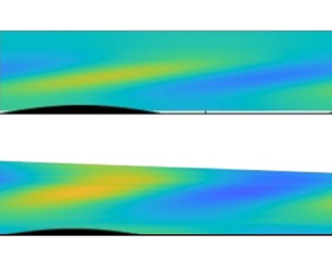
A shadowgraph visualisation of the flow above this plate is shown in figure 2(a). The flow is clearly fully turbulent from the very beginning of the plate (called ‘the leading edge’ in further discussion), with the presence of recirculation bubbles. In addition, the boundary layer is observed to separate from the surface, generating a black stripe (called ‘the front’ hereafter) evidenced by the white arrow in the shadowgraph. This effect is understood to be a consequence of lee waves generated by the leading edge, as the front position scales with $2{\rm \pi} U_\infty /N$. These waves could possibly generate an adverse pressure gradient leading to boundary layer separation. The undulation amplitude is also too large as it creates boundary layer separation after each crest.

Figure 2. Compilation of shadowgraph pictures of the flow above the entrance zone of the plate for two different leading edge profiles at towing speed $U_\infty =2.65\ {\rm cm}\ {\rm s}^{-1}$ and $N=1.06\pm 0.06\ {\rm rad}\ {\rm s}^{-1}$: (a) $\alpha =180^\circ$, $\gamma =0^\circ$; (b) $\alpha =168.7^\circ$, $\gamma =2^\circ$. The transverse angle $\alpha$ has been observed to have no influence on the boundary layer quality.

All of these issues have been solved by working on the design and position of the plate. First, the leading edge has been slimmed and shaped with a smooth curve on its downward part. Second, the whole plate has been inclined in its longitudinal direction at a very low angle $\gamma =2^\circ$ with respect to the horizontal. This forces the current lines to stay attached to the surface and strongly inhibits the generation of the so-called front. Finally, the undulation height $h$ has been reduced to 2.5 % of the wavelength $\lambda$.

The latter has been fixed to 10 cm so that the perturbation amplitude is not too small, but such that 5 complete undulations can still be shaped on the plate (the length of the plate is limited by the tank dimensions). The plane entrance zone has been fixed at 91 cm so that the boundary layer is of the largest possible extent. This eases visualisations and ensures that the undulations are indeed within the boundary layer extent.

The final plate is machined in black polyoxymethylene. A shadowgraph of the flow is presented in figure 2(b). The boundary layer flow is clearly nicer when compared with the first plate. No more turbulence is observed, the flow is laminar and follows almost all the undulations. Thin lines seem to be emitted from the plate but they do not correspond to a genuine boundary layer separation, as checked by PIV measurements. Note that shadowgraph visualisations do not show any evidence of a critical layer above the plate: this will require PIV.

2.5. Parameters of the study

This study presents results for a unique plate designed to optimise the formation of a critical layer, as has been discussed in the previous subsection. It is 141 cm long (including a plane entrance zone of 91 cm), 60 cm wide and 2 cm thick after the slim leading edge part. The undulations have a wavelength of $\lambda =10$ cm and a height $h=0.25$ cm. The transverse inclination angle $\alpha$ is kept constant and equal to $118.1^\circ$. The natural frequency associated with stratification is set to $N=0.85\pm 0.04\ {\rm rad}\ {\rm s}^{-1}$, by taking the mean density $\rho _0\sim 1.024\ {\rm g}\ {\rm cm}^{-3}$ as the reference density. These quantities lead to a constant theoretical critical velocity $U_c=\lambda N \sin \alpha /2{\rm \pi} =1.19\ {\rm cm}\ {\rm s}^{-1}$.

By fitting the measured longitudinal velocity at the mid-length of the undulations by $U_\infty F'(z/\delta _{emp})$ with $F$ defined in (3.7) (see § 3 for justification), an empirical boundary layer depth $\delta _{emp}$ is determined, varying between 0.58 and 0.75 cm (see table 1). It is the reference scale which will be used to non-dimensionalise lengths and to calculate the two non-dimensional parameters characterising the flow, namely the classical Reynolds $Re$ and Froude $Fr$ numbers,

(2.2a)$$\begin{gather} Re = U_\infty \delta_{emp}/\nu, \end{gather}$$

(2.2b)$$\begin{gather}Fr = U_\infty/N \delta_{emp}. \end{gather}$$

Table 1. Summary of experimental data. Here, $N=0.85\pm 0.04\ {\rm rad}\ {\rm s}^{-1}$, $\lambda =10$ cm and $\alpha =118.1^\circ$. The critical velocity $U_c= N \lambda \sin \alpha /(2{\rm \pi} )$ is equal to $1.19\ {\rm cm}\ {\rm s}^{-1}$.

The kinematic viscosity $\nu$ is $1.015 \pm 0.005.10^{-6}\ {\rm m}^2\ {\rm s}^{-1}$, as the salted water temperature is $T\sim 21.7\,^\circ {\rm C}$.

A summary of the parameters associated with each experiment is given in table 1.

3. Base flow

3.1. Theoretical developments

A stationary stratified boundary layer flow above a tilted wall is considered. This first section aims at properly calculating the base flow of this physical situation in the case $Re\gg 1$.

The wall is inclined in the cross-stream direction, such that its outward normal ${\boldsymbol {e}_{\boldsymbol {z}}}$ makes an angle $\alpha$ with the upward vertical $\boldsymbol {e}_{\boldsymbol {Z}}$, which is the stratification direction (see figure 1a).

The fluid is assumed to have both constant kinematic viscosity $\nu$ and Brunt–Väisälä frequency $N$, which is associated with a linear stable stratification

(3.1)\begin{equation} \varrho_{lin} = \varrho_0(1-N^2 Z/g), \end{equation}

where $g$ is the gravity. The diffusivity of the quantity generating the stratification is assumed to be very low compared with the viscosity of the fluid, such that its effect can be neglected. This is a valid assumption for brine solutions like the ones experimentally considered in this paper.

In the absence of motion, the balance between pressure and density terms prescribes

(3.2)\begin{equation} P_{lin} = \varrho_0 g Z\left(1-\frac{N^2}{2g} Z\right). \end{equation}

In the following, only pressure and density deviations from this hydrostatic equilibrium, denoted with a regular letter without an index, are considered.

From now, when no scaling is specified, velocities will be non-dimensionalised by $U_\infty$ (the uniform longitudinal velocity outside of the boundary layer), lengths by $\delta$ (the boundary layer width), pressures by $\varrho _0 U_\infty ^2$ and density by $\varrho _0 U_\infty ^2/g \delta$.

The dimensionless equations of motion, under the Boussinesq approximation, are

(3.3a)$$\begin{gather} \boldsymbol{\nabla}\boldsymbol{\cdot}\boldsymbol{u} = 0, \end{gather}$$

(3.3b)$$\begin{gather}(\boldsymbol{u}\boldsymbol{\cdot}\boldsymbol{\nabla})\boldsymbol{u} =- \boldsymbol{\nabla} p+\frac{1}{Re} \Delta \boldsymbol{u}- \rho \boldsymbol{e}_{\boldsymbol{Z}}, \end{gather}$$

(3.3c)$$\begin{gather}(\boldsymbol{u}\boldsymbol{\cdot}\boldsymbol{\nabla})\rho = \frac{\boldsymbol{u}\boldsymbol{\cdot}\boldsymbol{e_Z}}{Fr^2}, \end{gather}$$

where $p$ is the pressure and $\boldsymbol {u}$ is the dimensional velocity field, $u$, $v$ and $w$ being respectively the longitudinal, transverse and normal components in the plate reference frame.

Considering a transverse $\alpha$ angle forces the introduction of a transverse velocity $v$ as $\rho$ varies along the vertical $Z$ which includes components in both the $\boldsymbol {e}_z$ and $\boldsymbol {e}_y$ directions. This imposes a three-dimensional velocity field but as the wall is supposed infinite in the $\boldsymbol {e_y}$ direction, unknown functions can be kept independent of the $y$ variable.

By analogy with the classical Blasius problem on a flat plane $(x,z)$, we introduce the spatial scales

(3.4a,b)\begin{equation} x = Re \, \bar{x}, \quad z = \bar{z} , \end{equation}

and the scaling

(3.5a)$$\begin{gather} u_B = \bar{u}_B, \end{gather}$$

(3.5b)$$\begin{gather}v_B = \displaystyle Re^{-1} \bar{v}_B, \end{gather}$$

(3.5c)$$\begin{gather}w_B = \displaystyle Re^{-1} \, \bar{w}_{B}, \end{gather}$$

(3.5d)$$\begin{gather}p_B = Re^{-2} \, \bar{p}_{B}, \end{gather}$$

(3.5e)$$\begin{gather}\rho_B = Re^{-2} \, \bar{\rho}_B, \end{gather}$$

where the ‘$B$’ index has been added to refer to the Blasius base flow.

Using these equalities, the complete system (3.4a,b) can thereby be reduced at leading order to

(3.6a)$$\begin{gather} \frac{\partial \bar{u}_B}{\partial \bar{x}}+\frac{\partial \bar{w}_B}{\partial \bar{z}} =0, \end{gather}$$

(3.6b)$$\begin{gather}\bar{u}_B\frac{\partial \bar{u}_B}{\partial \bar{x}}+\bar{w}_B\frac{\partial \bar{u}_B}{\partial \bar{z}} =\displaystyle \frac{\partial^2 \bar{u}_B}{\partial \bar{z}^2}, \end{gather}$$

(3.6c)$$\begin{gather}\bar{u}_B\frac{\partial \bar{v}_B}{\partial \bar{x}}+ \bar{w}_B \frac{\partial \bar{v}_B}{\partial \bar{z}} =-\bar{\rho}_B\sin\alpha + \displaystyle \frac{\partial^2 \bar{v}_B}{\partial \bar{z}^2} \end{gather}$$

(3.6d)$$\begin{gather}\bar{u}_B\frac{\partial \bar{w}_B}{\partial \bar{x}}+\bar{w}_B \frac{\partial \bar{w}_B}{\partial \bar{z}}=- \displaystyle \frac{\partial \bar{p}_B}{\partial \bar{z}}- \bar{\rho}_B \cos\alpha+\displaystyle \frac{\partial^2 \bar{w}_B}{\partial \bar{z}^2}, \end{gather}$$

(3.6e)$$\begin{gather}\bar{u}_B\frac{\partial \bar{\rho}_B}{\partial \bar{x}}+\bar{w}_B \displaystyle \frac{\partial \bar{\rho}_B}{\partial \bar{z}} = \displaystyle \frac{Re^2}{Fr^2} \left(\cos\alpha\bar{w}_B +\sin\alpha\bar{v}_B\right), \end{gather}$$

where it is implicitly assumed that $Re/Fr$ and $\alpha$ are $O(1)$.

The two first equations (3.6a,b) correspond to the classical system governing a Blasius boundary layer (e.g. Schlichting 1979). They constitute an independent system for the two velocity components $\bar {u}_B$ and $\bar {w}_B$ that can be solved in term of a self-similar variable $\eta =\bar {z}/\sqrt {\bar {x}}$ using a single function $F(\eta )$ satisfying

(3.7)\begin{equation} 2F'''+F''F=0, \end{equation}

with the boundary conditions: $F'(0)=F(0)=0$ and $F'(\eta \rightarrow \infty )=1$ (a prime denotes a derivative with respect to $\eta$). The relation between $F(\eta )$ and the velocity components $\bar {u}_B$ and $\bar {w}_B$ is

(3.8a)$$\begin{gather} \bar{u}_{B}= F', \end{gather}$$

(3.8b)$$\begin{gather}\bar{w}_{B} = \frac{\eta F' - F}{2 \sqrt{\bar{x}}}. \end{gather}$$

Observing now the rest of system (3.6) suggests the origin of the other scalings: the one for $v$ is the same as for $w$ because of (3.6e), which forces the scaling for $\rho$ in (3.6c), itself leading to the scaling for $p$ in (3.6d).

In the present paper, we shall present experimental results obtained for a fixed angle $\alpha =118.1^\circ$ and Froude numbers of the order of unity. We shall therefore be in the limit $Re \gg Fr$ for which the last equation (3.6e) reduces to the right-hand side. This means that the transverse and normal velocities will be proportional in order to cancel the vertical velocity. Streamlines will remain horizontal, as is often the case in stratified fluids. In this large $Re/Fr$ limit, the transverse velocity associated with the Blasius flow will therefore be

(3.9)\begin{equation} \bar{v}_B =-\frac{\cos\alpha}{\sin\alpha}\bar{w}_{B} ={} -\frac{\cos\alpha}{\sin\alpha}\frac{\eta F' - F}{2 \sqrt{\bar{x}}}. \end{equation}

Once $\bar {v}_B$ is calculated, the density field $\bar {\rho }_B$ is obtained through (3.6c). The Blasius equation (3.7) is needed to simplify some terms, such that one can write

(3.10)\begin{equation} \bar{\rho}_B =\frac{\cos{\alpha}}{\sin^2{\alpha}} \frac{F'F -\eta F'^2 -2 F'' }{4\bar{x}^{3/2}}. \end{equation}

Combining (3.6c) and (3.6d) with (3.9) allows us to express the pressure gradient as a function of the density only

(3.11)\begin{equation} \frac{\partial \bar{p}_B}{\partial \bar{z}} =-\frac{1}{\cos{\alpha}}\bar{\rho}_B, \end{equation}

and obtain

(3.12)\begin{equation} \bar{p}_B =\frac{1}{\bar{x}\sin^2{\alpha}}\left(2 F' - \frac{F^2}{2} + \int^\eta s F'^2(s)\,{\rm d}s\right). \end{equation}

The system (3.6a–e) has now been fully solved in the experimental parameter range, that is: finite $\sin {\alpha }$, $Fr$ of order one and large $Re$. These solutions are plotted in figure 3 as a function of the normal component. Interestingly, the normal and transverse velocity components and the density perturbation do not vanish at infinity but rather converge toward a finite value. The pressure increases linearly at large $\bar {z}$.

Figure 3. Normal profiles of the longitudinal velocity (a), the normal and transverse velocity (b), the density (c) and the pressure (d). Solid black lines correspond to the stratified Blasius solution (3.8)–(3.12) for $\bar {x}=1$ with $F$ the solution of (3.7). In (a), blue dotted symbols correspond to the experimental longitudinal velocity $u$ at the end of the plane entrance zone (86 cm from the front edge) for experiment number 5 (see table 1) with $z$ dimensionalised by $\delta _{fit}=0.49$ cm and the red dashed line corresponds to the Falkner–Skan solution (3.13) for $\bar {x}=1.1$ with a tilt angle $\gamma =2^\circ$.

In Appendix A, we provide some information on another limit, obtained when $\alpha \rightarrow 0$ or $Fr$ large, that can also be solved explicitly.

3.2. Comparison with experimental measurements

As detailed in § 2.3, a PIV technique has been set up to measure both longitudinal and transverse velocity fields ($u$ and $v$). Without undulations, the transverse velocity $v$ scales as $Re^{-1}$ and is thus too small to be measurable. Only the longitudinal velocity $u$ has therefore been measured. It has been plotted for experiment 5 in figure 3 where it is also compared with the theoretical Blasius solution.

The experimental measurement has been taken 5 cm before the start of the undulations, after the boundary layer has developed over $L=86$ cm from the front edge. A good agreement is observed between the theoretical and experimental profiles, as figure 3 shows. For $\bar {z}<0.9$, the reflexion of the laser on the plate creates a bright area on the images which perturbs the PIV measurements and leads to wrong velocities. Above the laser reflexion zone, for $\bar {z}>0.9$, both profiles match with a maximum uncertainty of the order of 5 %, which confirms the base flow theoretical profile. The spatial diffusion of the boundary layer due to viscous effects suggests that the boundary layer width should be $\delta _{theo}=\sqrt {\nu L /U_\infty }=0.58$ cm, which is larger than the $\delta _{fit}=0.49$ cm obtained in figure 3 from the best fit. A similar difference between fitting and theoretical prediction of the order of 20 % is observed for all performed experiments. This difference partly comes from the small longitudinal tilt angle $\gamma =2^\circ$ of the plate. Indeed, in the absence of stratification, the streamwise velocity above a tilted plate is given by the Falkner–Skan solution (Drazin & Reid 1999)

(3.13)\begin{equation} \bar{u}_B=F_{FS}'\left(\frac{\bar{z}}{\bar{x}^{(1-m)/2}} \sqrt{\frac{m+1}{2}} \right) \quad \mathrm{with}\ F_{FS}'''+F_{FS}F_{FS}''+\beta |1-F_{FS}'^2|=0 \end{equation}

where $\beta =2 \gamma /180$ and $m=\beta /(2-\beta )$. As shown in figure 3(a), this solution is almost undistinguishable from the Blasius solution if $\bar {x}$ is increased by 10 %. This means that the tilt angle $\gamma =2^\circ$ decreases the thickness by 5 %, which is thus equal practically to $0.55$ cm rather than $0.58$ cm. This prediction is closer to the measured thickness $\delta _{fit}=0.49$ cm although it is still 10 % larger. The remaining difference probably comes from the rounded leading edge.

For the final plots and the calculation of quantitative predictions presented in § 4.3, the thickness $\delta _{emp}$ is measured by fitting the longitudinal profile with the Blasius profile in the middle of the sinusoidal part of the plate, rather than upstream of the undulations as done here for $\delta _{fit}$. It has been checked that the longitudinal flow is not modified by the undulations and that it still matches the Blasius profile. The empirical values are given in table 1.

4. Perturbed flow

4.1. Experimental transverse velocity field

The tilt angle of the plate breaks the invariance along the $y$ direction and induces a transverse velocity $v$ which is enhanced by the plate undulations. This allows its measurement by PIV. A raw transverse velocity field is displayed in figure 4. The undulations are darkened to ease the visualisation.

Figure 4. Raw data of the transverse velocity field above the plate for experiment number 4.

First, one can note that the transverse velocity is still very weak. Indeed, its amplitude is of the order of only $5\,\%$ of the maximum longitudinal velocity $U_\infty$. This measurement was thus extremely hard to achieve since the noise had to be reduced below 1 %. The fine post-processing described in § 2.3 was necessary to obtain such an accuracy.

Then, one can observe in this field alternate bands of $v$ above the plate upstream of the undulated part. As was shown in Christin (2021), these waves are orographic waves emitted by the front edge. They are of no interest for the present study.

Now, focusing on the field above the undulations, inclined lobes of alternating positive and negative transverse velocity can clearly be identified. They are within the boundary layer and exhibit the wavelength of the undulations. This pattern becomes more pronounced downstream: two undulations seem to be sufficient to settle this oscillating regime forced by the topography.

Although the orographic waves have a smaller amplitude than the inclined lobes, they are not negligible. To better reveal the lobes, data are then filtered with a spatial Fourier filter along $\tilde {x}$ at the wavenumber of the undulations in figure 5, which shows 3 wavelengths to give a more detailed image of the velocity field. The Fourier-filtered velocity is obtained as

(4.1)\begin{equation} v_c(\bar{z})\cos(k\tilde{x})+v_s(\bar{z})\sin(k\tilde{x}), \end{equation}

where for each $\bar {z}$ the Fourier coefficients are defined as

(4.2)\begin{equation} v_c(\bar{z})=\left.\int_{x_{min}}^{x_{max}}v(\tilde{x},\bar{z})\cos(k\tilde{x})\, {\rm d}\tilde{x}\right/\int_{x_{min}}^{x_{max}}\cos^2(k\tilde{x})\,{\rm d}\tilde{x}, \end{equation}

and

(4.3)\begin{equation} v_s(\bar{z})=\left.\int_{x_{min}}^{x_{max}}v(\tilde{x},\bar{z})\sin(k\tilde{x}) \,{\rm d}\tilde{x}\right/\int_{x_{min}}^{x_{max}}\sin^2(k\tilde{x})\,{\rm d}\tilde{x}, \end{equation}

with $x_{min}$ the starting point of the undulations and $x_{max}$ the largest position where experimental data are available. The specific pattern develops slightly above the surface of the plate, around $\bar {z}=1$, and has velocity lobes inclined with a small positive angle with respect to the horizontal. Positive lobes are located above the ridge of the undulation whereas negative lobes are located above the depression.

Figure 5. Transverse velocity field for experiment number 4, after applying a Fourier filter at the wavelength of the undulations along $\tilde {x}$.

This measured transverse field corresponds to the perturbed transverse flow induced by the undulations. This pattern, which is localised away from the boundary, is reminiscent of a critical layer singularity (Passaggia et al. 2014). In the next section, we provide a complete theory explaining the presence of this pattern. The theory developed in Passaggia et al. (2014) is extended to account for a no-slip boundary condition and applied to the Blasius profile configuration for a quantitative comparison.

4.2. Theoretical developments

The base flow is perturbed with low-amplitude (i.e. $h\ll 1$) undulations of the plate, parametrised with a sine function of wavenumber $k =O(1)$ (the wavelength is assumed to be of the same order as the boundary layer width). It is also assumed that the length over which the boundary layer has developed before arriving on the corrugations is large enough so that the boundary layer flow is settled and its width is approximatively constant for the extent of the undulations. The slow longitudinal variable $\bar {x}$ of the Blasius boundary layer is now related to a local variable $\tilde {x}$

(4.4)\begin{equation} \tilde{x}=Re(\bar{x}-1)=x-Re. \end{equation}

The location $\bar {x}=1$ (where $\eta = z$) corresponds to the position in the middle of the undulations. It is here that the boundary layer width $\delta _{emp}$ has been estimated and where the flow is analysed.

Perturbations being searched as spatial Fourier modes, physical quantities are written as

(4.5a)$$\begin{gather} \boldsymbol{u_{tot}} = \boldsymbol{u_B} + \tfrac{1}{2}hk \left(\boldsymbol{u}{\rm e}^{{\rm i}k \tilde{x}}+ \mathrm{c.c.}\right), \end{gather}$$

(4.5b)$$\begin{gather}\,p_{tot} = \,p_{lin}+ p_B + \tfrac{1}{2}hk \left( p {\rm e}^{{\rm i}k \tilde{x}}+ \mathrm{c.c.}\right), \end{gather}$$

(4.5c)$$\begin{gather}\rho_{tot} = \rho_{lin} + \rho_B + \tfrac{1}{2}hk \left(\rho {\rm e}^{{\rm i}k \tilde{x}}+ \mathrm{c.c.} \right), \end{gather}$$

where $\boldsymbol {u}$, $\rho$ and $p$ are functions of the normal spatial variable $z$ only.

In the bulk of the boundary layer (that is for $z=O(1)$), the perturbations are expected to be described by inviscid equations. This region corresponds to the inviscid outer layer in the sketch of the different regions shown in figure 6. Viscous effects are present in two localised regions. Very close to the surface of the plate, in a viscous sub-layer, they are needed to apply the no-slip boundary condition at the surface of the plate. The width of this layer is obtained by balancing inertial and viscous effects. For a flat plate, this width is $O(Re^{-1/3})$ owing to the presence of a regular critical point at the wall (i.e. $U_B(0) = \omega /k =0$) (see Drazin & Reid 1999). For an undulated plate, we obtain the same width scaling as long as $h\ll Re^{-1/3}$. The solution of this viscous sub-layer will provide the boundary conditions for the inviscid outer solution. Viscous effects will also be needed in the baroclinic critical layer to smooth the singularity that appears in the inviscid solution.

Figure 6. Scheme of the different layers studied.

4.2.1. The viscous sub-layer

In order to describe the perturbation in a viscous sub-layer of $O(Re^{-1/3})$ width, it is natural to introduce the new normal variable

(4.6)\begin{equation} \tilde{z} = \frac{ z - h \sin{ k \tilde{x} } } {Re^{-1/3}}, \end{equation}

such that $\tilde {z}=0$ corresponds to the deformed boundary. As mentioned above, we further assume that $h\ll Re^{-1/3}$ such that the problem remains linear at leading order. In the viscous sub-layer, velocity, pressure and density perturbations are expanded as

(4.7a)$$\begin{gather} u = \tilde{u}, \end{gather}$$

(4.7b)$$\begin{gather}v = Re^{-1/3} \tilde{v}, \end{gather}$$

(4.7c)$$\begin{gather}w = Re^{-1/3} \tilde{w}, \end{gather}$$

(4.7d)$$\begin{gather}p = Re^{-1/3} \tilde{p}, \end{gather}$$

(4.7e)$$\begin{gather}\rho = Re^{-2/3} \tilde{\rho}. \end{gather}$$

The boundary conditions on the velocity perturbations are obtained by expanding $\bar {u}_B$ close to the boundary

(4.8)\begin{equation} \bar{u}_B \sim \bar{u}'_{B_0} \eta= \bar{u}'_{B_0} \left( \tilde{z}\,Re^{-1/3}+h\sin{k \tilde{x} } \right), \end{equation}

where $\bar {u}'_{B_0}$ stands for the derivative of $\bar {u}_B$ with respect to $\eta$ for $\eta =0$. The boundary condition ${\boldsymbol {u}_{\boldsymbol {tot}}}(\tilde {z}=0)=0$ then gives

(4.9a–c)\begin{equation} \tilde{u}(0) = \frac{{\rm i}\,\bar{u}'_{B_0}}{k}, \quad \tilde{v}(0) =0, \quad \tilde{w}(0) =0. \end{equation}

Now introducing (4.7) and (4.8) in the governing equations (3.4a,b) the following non-dimensionalised system is obtained:

(4.10a)$$\begin{gather} {\rm i} k \tilde{u} + \frac{{\rm d} \tilde{w}}{{\rm d} \tilde{z}} =0, \end{gather}$$

(4.10b)$$\begin{gather}{\rm i} k \tilde{u} \bar{u}'_{B_0} \tilde{z}+ \tilde{w} \bar{u}'_{B_0} =-{\rm i} k\tilde{p} + \frac{{\rm d}^2 \tilde{u}}{{\rm d} \tilde{z}^2}, \end{gather}$$

(4.10c)$$\begin{gather}{\rm i} k \tilde{v} \bar{u}'_{B_0} \tilde{z} +\tilde{\rho} \sin{\alpha} = \frac{{\rm d}^2 \tilde{v}}{{\rm d} \tilde{z}^2}, \end{gather}$$

(4.10d)$$\begin{gather}\frac{{\rm d} \tilde{p}}{{\rm d} \tilde{z}} = 0, \end{gather}$$

(4.10e)$$\begin{gather}\tilde{v} \sin{\alpha} + \tilde{w} \cos{\alpha} = 0. \end{gather}$$

Differentiation of (4.10b) with respect to $\tilde {z}$ yields a homogeneous Airy equation on ${\rm d} \tilde {u}/{\rm d} \tilde {z}$

(4.11)\begin{equation} \frac{{\rm d}^3 \tilde{u}}{{\rm d} \tilde{z}^3} - {\rm i} k \bar{u}'_{B_0} \tilde{z}\frac{{\rm d} \tilde{u}}{{\rm d} \tilde{z}} = 0. \end{equation}

Without surprise, we obtain the equation describing perturbations in a viscous critical layer (Drazin & Reid 1999). As already mentioned above, this comes from the fact that the position $z=0$ is a regular critical point for the stationary perturbations generated by the wall undulations. Such a critical layer at the wall is also obtained in the asymptotic structure of Tollmien–Schlichting waves in the lower branch of the stability diagram (Lin 1955). It also corresponds to the lower deck obtained in the triple deck theory describing boundary layer separation (Smith 1973; Wu & Zhang 2008a; Dong, Liu & Wu 2020).

Solving this equation allows us to obtain $\tilde {u}$, which gives $\tilde {w}$ thanks to (4.10a), then $\tilde {v}$ through (4.10e), the constant $\tilde {p}$ using (4.10b) and finally $\tilde {\rho }$ using (4.10c).

As explained in the appendix of Drazin & Reid (1999) textbook, recessive solutions of homogeneous Airy equations such as (4.11) can be expressed in terms of generalised Airy functions $A_k(z,p)$, where $p$ denotes the integral order (if $p>0$) of the Airy function. The longitudinal velocity $\tilde {u}$ is then searched under the form

(4.12)\begin{equation} \tilde{u} = C_0 A_1(\beta {\rm e}^{{\rm i} {\rm \pi}/6} \tilde{z},1)+C_1, \end{equation}

with $C_0$ and $C_1$ being two complex constants, and

(4.13)\begin{equation} \beta=(k \bar{u}'_{B_0})^{1/3}. \end{equation}

Applying the boundary conditions (4.9a–c), the system (4.10a–e) can then be fully solved. The solution in the viscous sub-layer is found to be

(4.14a)$$\begin{gather} \tilde{u}(\tilde{z}) = \frac{{\rm i}\bar{u}'_{B_0}}{k} \frac{A_1(\beta^{1/3} {\rm e}^{{\rm i} {\rm \pi}/6} \tilde{z},1)}{A_1(0,1)}, \end{gather}$$

(4.14b)$$\begin{gather}\tilde{v}(\tilde{z}) =- \cot{\alpha} \beta^{-1}\bar{u}'_{B_0} {\rm e}^{-{\rm i} {\rm \pi}/6}\frac{A_1(\beta {\rm e}^{{\rm i} {\rm \pi}/6} \tilde{z},2)-A_1(0,2)}{A_1(0,1)}, \end{gather}$$

(4.14c)$$\begin{gather}\tilde{w}(\tilde{z}) = \beta^{-1}\bar{u}'_{B_0} {\rm e}^{-{\rm i} {\rm \pi}/6}\frac{A_1(\beta {\rm e}^{{\rm i} {\rm \pi}/6} \tilde{z},2)-A_1(0,2)}{A_1(0,1)}, \end{gather}$$

(4.14d)$$\begin{gather}\tilde{p}(\tilde{z}) =-\frac{\beta^{2} \bar{u}'_{B_0}}{k^2}\frac{A_1(0,2)}{A_1(0,1)}{\rm e}^{{\rm i} {\rm \pi}/3}, \end{gather}$$

(4.14e)$$\begin{gather}\tilde{\rho}(\tilde{z}) = \frac{\cos{\alpha} \beta \bar{u}'_{B_0}}{\sin^2{\alpha}} \frac{{\rm i} \beta {\rm e}^{-{\rm i} {\rm \pi}/6} \tilde{z} \left(A_1(\beta {\rm e}^{{\rm i} {\rm \pi}/6} \tilde{z},2)-A_1(0,2) \right)-{\rm e}^{{\rm i} {\rm \pi}/6}A_1(\beta {\rm e}^{{\rm i} {\rm \pi}/6} \tilde{z})}{A_1(0,1)}. \end{gather}$$

As explained above, from this solution, we can obtain the boundary conditions to apply to the outer solution. The condition of matching implies that the sub-layer solution as $\tilde {z} \rightarrow \infty$ should correspond to the inviscid outer solution as $z\rightarrow 0$.

Using the property that $\mathop {z \rightarrow \infty }\nolimits _{lim} A_1(z,2) = 0$ and relations between $A_1(0,p)$ and the $\varGamma$ function (see Drazin & Reid 1999), we, in particular, obtain the value of the normal velocity of the outer solution at the wall that should be given by

(4.15)\begin{equation} {w(0)= \displaystyle{\underset{\tilde{z} \rightarrow \infty}{\mathrm{lim}} Re^{-1/3} \tilde{w}} = Re^{-1/3} \displaystyle{\frac{\beta^{-1}\bar{u}'_{B_0} }{3^{1/3}\varGamma(4/3)}{\rm e}^{-{\rm i} {\rm \pi}/6}}. } \end{equation}

4.2.2. The outer layer

The inviscid layer lying above the viscous sub-layer, the so-called outer layer, has been studied by Passaggia et al. (2014): it is in this region that the baroclinic critical layer appears. In Passaggia et al. (2014), the normal velocity that was forcing the solution in the outer layer was $O(1)$ and proportional to a prescribed longitudinal velocity. Here, it is obtained from the condition of matching with the viscous sub-layer. It is therefore weaker and of order $Re^{-1/3}$ as prescribed by (4.15).

In the outer layer, velocity, pressure and density perturbations vary with respect to the spatial variables $\tilde {x}$ and $\bar {z}$, both non-dimensionalised with $\delta$ and exhibit a scaling prescribed by the matching with the sub-layer

(4.16)\begin{equation} (\boldsymbol{u},\rho,p) = Re^{-1/3} (\hat{\boldsymbol{u}},\hat{\rho},\hat{p}). \end{equation}

Despite the amplitude factor, the analysis of Passaggia et al. (2014) can still be applied. One just has to consider a Blasius base flow instead of the $\tanh$ profile they considered. As shown in that paper, one obtains after manipulating the system (3.4a,b) a single (Rayleigh) equation for the normal velocity $\hat {w}$

(4.17)\begin{equation} \frac{{\rm d}^2 \hat{w}}{{\rm d} \bar{z}^2}-\frac{\bar{u}''_{B}}{\bar{u}_{B}}\hat{w}-k^2\frac{1-(k\bar{u}_{B} Fr)^2}{\sin{}^2\alpha-(k\bar{u}_{B}Fr)^2} \hat{w}=0. \end{equation}

The boundary condition at $\bar {z}=0$ is now rigorously prescribed by the condition $\hat {w}(0)={\tilde {z} \rightarrow \infty }_{lim} \tilde {w}$ which, thanks to (4.15), gives

(4.18)\begin{equation} \displaystyle{\hat{w}(0)} = \displaystyle{\frac{\beta^{-1}\bar{u}'_{B_0} }{3^{1/3}\varGamma(4/3)}{\rm e}^{-{\rm i} {\rm \pi}/6}}. \end{equation}

The other condition at infinity is that the perturbation should either vanish or be an outgoing wave. These conditions at $\bar {z}$ equal to zero and infinity fully determine the function $\hat {w}$ if one knows how to treat the branch point singularity present at the position $\bar {z}_c$ where

(4.19)\begin{equation} \left(k\bar{u}_{B}(\bar{z}_c)Fr \right)^2=\sin^2{\alpha}. \end{equation}

At this point, the function $\hat {w}$ is finite but its derivative $\hat {w}'$ exhibits a logarithmic singularity. As explained in Passaggia et al. (2014), this logarithmic function can be defined as in the classical stability theory (Lin 1955): the branch cut should be fixed in the upper complex plane (because $\bar {u}'_{Bc} >0$). This means that the singularity can be avoided by integrating (4.17) in the lower complex plane above the singular point.

Once $\hat {w}$ is obtained, the other components can be deduced from it. For the transverse velocity $\hat {v}$ and the density $\hat {\rho }$, we get

(4.20a)$$\begin{gather} \hat{v} = \displaystyle{-\frac{\sin{\alpha} \cos{\alpha}\, \hat{w}}{\sin^2 \alpha-(k\bar{u}_{B}Fr)^2}}, \end{gather}$$

(4.20b)$$\begin{gather}\hat{\rho} = \displaystyle{\frac{{\rm i} k\bar{u}_{B}\cos{\alpha}\, \hat{w}}{\sin^2\alpha-(k\bar{u}_{B}Fr)^2}}. \end{gather}$$

By contrast with $\hat {w}$, which remains finite at $r_c$, the outer expressions (4.20a,4.20b) of $\hat {v}$ and $\hat {\rho }$ are singular at $r_c$. The singularity is therefore stronger than at a regular critical point. It corresponds to a so-called baroclinic critical point (e.g. Wang & Balmforth 2020). It is associated with a local resonance of the inertial frequency $\omega - k \bar {u}_{B}$ of the perturbation (where the forcing frequency $\omega$ vanishes in our case since the undulations are stationary) with the local Brunt–Väisälä frequency $\pm N \sin \alpha$ in the shear plane. As for a regular critical layer, the regularisation of the solution is possible by considering viscous effects in a small region of width $O(Re^{-1/3})$ around the baroclinic critical point. This region corresponds to the viscous baroclinic critical layer.

4.2.3. The viscous baroclinic critical layer

This part is formally strictly equivalent to the one presented by Passaggia et al. (2014) and the reader is advised to refer to this article to have more details on the analysis.

To describe the fields in the vicinity of the critical position $\bar {z}_c$, viscous effects need to be reintroduced to smooth out the singularity. The scaling becomes

(4.21a)$$\begin{gather} u = Re^{-1/3}\check{u}(\check{z}), \end{gather}$$

(4.21b)$$\begin{gather}v = \check{v}(\check{z})+Re^{-1/3}\check{v}_s(\check{z}), \end{gather}$$

(4.21c)$$\begin{gather}w = Re^{-1/3}\hat{w}_c+Re^{-2/3}\check{w}(\check{z}), \end{gather}$$

(4.21d)$$\begin{gather}p = Re^{-1/3}\check{p}(\check{z}), \end{gather}$$

(4.21e)$$\begin{gather}\rho = \check{\rho}(\check{z})+Re^{-1/3}\check{\rho}_s(\check{z}), \end{gather}$$

where $\check {z}= (\bar {z}-\bar {z}_c)Re^{1/3}$ is the critical layer variable.

By introducing this scaling in the governing equations (3.4a,b), one can show that the system can be reduced to an inhomogeneous Airy equation for $\check {v}$

(4.22)\begin{equation} \frac{{\rm d}^2 \check{v}}{{\rm d} \check{z}^2}- 2 {\rm i} k \bar{u}'_{Bc} \check{v}\check{z} =-\frac{{\rm i} \hat{w}_c\,\mathrm{sign}(\sin{\alpha}) \cos{\alpha}}{Fr}, \end{equation}

where $\bar {u}'_{Bc}$ is the derivative of $\bar {u}_B$ with respect to $\eta$, evaluated at the critical position $\bar {z}_c$. The other velocity components, the pressure and the density are then given by

(4.23a)$$\begin{gather} \check{\rho} =-{\rm i} \frac{\check{v}}{Fr} , \end{gather}$$

(4.23b)$$\begin{gather}\frac{{\rm d}\check{p}}{{\rm d}\check{z}} = {\rm i} \cos\alpha \check{\rho}, \end{gather}$$

(4.23c)$$\begin{gather}\bar{u}_{Bc} \check{u} = \check{p} + {\rm i} \frac{\tilde{w}_c \bar{u}'_{Bc} }{ k} , \end{gather}$$

(4.23d)$$\begin{gather}\frac{{\rm d}\check{w}}{{\rm d}\check{z}} =-{\rm i} k \check{u}. \end{gather}$$

Note that the $\log (Re)$ correction terms that were provided in Passaggia et al. (2014) are here implicitly included in each expression.

To solve (4.22), it is convenient to introduce the generalised Airy functions $B_k(z,0)$ (see Drazin & Reid 1999), that satisfy the inhomogeneous Airy equation

(4.24)\begin{equation} \left( \frac{{\rm d}^2 }{{\rm d} z^2} - z \right)B_k(z,0) =1, \end{equation}

and behave as $1/z$ for large $|z|$ (for particular values of ${\rm arg}(z)$) to be able to match with the solution in the outer region. An adequate choice of the cubic root of $2{\rm i} k \bar {u}'_{Bc}$ allows us to use the function $B_1(z,0)$ and write the solution as

(4.25)\begin{equation} \check{v} = \frac{{\rm i} \hat{w}_c \,\mathrm{sign}(\sin{\alpha}) \cos{\alpha}}{\left( 2 k\bar{u}'_{Bc} \right)^{2/3}Fr} B_1(-{\rm i} ( 2 k\bar{u}'_{Bc} )^{1/3}\check{z},0). \end{equation}

As $\check {z} \rightarrow \pm \infty$, this expression satisfies

(4.26)\begin{equation} \check{v} \sim \check{v}_{ceq} \equiv- \frac{\hat{w}_c \,\mathrm{sign}(\sin{\alpha}) \cos{\alpha}}{\left( 2 k\bar{u}'_{Bc} \right)Fr \check{z}}, \end{equation}

and thus matches with (4.20a) as $\bar {z}\rightarrow \bar {z}_c$.

4.3. Comparisons between experimental and theoretical results

4.3.1. Qualitative comparison of transverse velocity fields

Sections 4.2.1 to 4.2.3 give the complete solution of the perturbed flow. To compare the theoretical predictions with the experimental measurements, we use for the transverse velocity a composite expression obtained from expressions (4.20a) and (4.25) in the outer region and in the critical layer

(4.27)\begin{equation} \check{v}_p=\frac{\hat{v} \check{v}}{\hat{v}_{ceq}}, \end{equation}

where $\check {v}_{ceq}$ is defined in (4.26).

Resulting theoretical fields are presented in figure 7(a) to directly be compared with the corresponding experimental ones obtained thanks to a spatial Fourier filter applied to PIV data as introduced in § 4.1.

Figure 7. Theoretical ($v_p$) and Fourier-filtered experimental transverse velocity fields for two wavelengths of experiment numbers 2, 4 and 6 (from the top to the bottom). For details see table 1. The four other fields are presented in Christin (2021).

It is important to emphasise that the theory has no adjustable parameter except the boundary layer width $\delta$, which is slightly modified to better fit with the base flow profile.

Even in the absence of direct fitting, a good qualitative agreement is observed in figure 7 between the experimentally measured fields and the ones predicted by the theory. Indeed, the inclined lobes of alternating positive and negative transverse velocity generated slightly away from the plate surface are captured. Whereas the theoretical critical layer is thinner than the one effectively observed, both fields show a constant inclination angle ${\varOmega }$ (around $10^\circ$) of the lobes, which are located at a position that gets closer to the plate surface when the towed velocity increases (from experiment 2 to 6). The order of magnitude also seems to be recovered.

4.3.2. Quantitative results

These qualitative agreements can be quantitatively checked.

In order to do so, filtered and theoretical transverse velocity profiles along the normal axis $\bar {z}$ of a typical experiment (number 4 in table 1) are plotted in figure 8. The first two graphs, shown in (a,b), correspond to the profile at two specific longitudinal positions ($\tilde {x}=\lambda /4\delta$ and $0$, respectively) where the imaginary part and the real part of the transverse velocity should be obtained according to the theory. The third graph, shown in (c), presents the norm of $v$. Note that the theoretical position of the maximum of $|v|$ is slightly smaller than $\bar {z}_c$. This is due to the moderate value of the Reynolds number and the decreasing behaviour of the outer solution $|\hat {v}|$. These plots show some previously noted deviations between data such as the larger extent of the experimental critical layer compared with the predicted one, especially visible in (b,c). Also, an amplitude difference of the order of $50\,\%$ is also observed in (c): the amplitude of the velocity in the critical layer is larger than expected. However, the distance from the plate at which the critical layer starts is remarkably well predicted, as well as its first half-profile (up to $\bar {z}\sim 1.5$), which is particularly striking in the second plot. This better agreement for a lower $\bar {z}$ position could be explained by the larger amount of experimental data over which the Fourier filter is applied at these heights. Indeed, as it can be seen in figure 4, the visual range is more and more cropped away from the plate as $\tilde {x}$ increases, so that the complete velocity field over the whole critical layer is only obtained on the first undulations (especially for lower towing velocity experiments). Furthermore, it is on these early undulations (especially the first two as can be seen in figure 4) that the critical layer settles: then the filtered profile resulting from this first part is expected to deviate from the theoretical prediction.

Figure 8. Filtered (dots) and theoretical (full lines) transverse velocity profiles for experiment number 4 for two $\tilde {x}$ positions and the norm.

To have a more systematic comparison for each experiment, four characteristic quantities are defined in figure 9 and plotted in figure 10. The first one is the position of the critical layer $\bar {z}_c$ experimentally defined as the $\bar {z}$ position of the norm maximum value, itself corresponding to the second checked quantity. The third one is the angle ${\varOmega }$ made by the velocity lobe with respect to the plate surface, and the last one is the phase $\varphi _{max}$ indicating the relative position of the lobes compared with the undulations.

Figure 9. Scheme defining the quantities experimentally measured and theoretically computed for comparison in figure 10.

Figure 10. Quantitative comparison between quantities extracted from experimental and theoretical results. For theoretical lines, the mean value $Re=148$ (and $k=0.40$ for the continuous line) are used. Dotted lines correspond to the minimum and maximum $k$ experimentally considered.

Again, theoretical and experimental results show a good agreement, especially considering the completeness of the theory that does not require any direct fitting between data.

Panel (a) confirms the lowering position of the critical layer with the increase of $kFr$ (and then in $U_\infty$ as it is the only varying parameter). It goes from $+\infty$ when $kFr \rightarrow \sin {\alpha }$ (i.e. $U_\infty$ tends to the critical velocity), to 0 when $kFr$ increases. This can be easily understood as the critical velocity (kept constant in these experiments as $k$, $N$ and $\alpha$ are fixed) is reached for smaller $\bar {z}$ when the boundary layer profile has to match a higher velocity at ‘infinity’. Experimental values all lie above the theoretical line. This could be explained by the fact that the Blasius boundary layer is not a perfect model above the undulations which tend to widen the boundary layer thickness by generating a larger normal velocity than expected above a plane wall. Still, experimental values are close to the theoretical line and seem to validate the model.

Concerning the critical layer amplitude (panel b), the theoretical predicted value is globally smaller than the one observed, but the model seems more and more accurate with increasing $kFr$. The stronger deviation for lower towing velocity experiments could be explained by the same phenomenon as discussed above concerning the cropped visual range. However, considering the range of potential theoretical values suggested by the dotted lines, indicating the extreme $k$ values experimentally studied, the model seems to catch the essence of the critical layer amplitude behaviour.

The lower graphs show the phase $\varphi _{max}$ (c) and the inclination angle ${\varOmega }$ of the lobes (d) which are theoretically expected to be constant for $kFr>1.4$, that is in global agreement with experimental measurements.

5. Conclusion

In this paper, a coupled theoretical and experimental approach has been presented to study a stratified boundary layer above an inclined sinusoidal wall.

The experimental study of a stratified boundary layer generated by a towing plate has been found to be particularly challenging. The shape of the leading edge of the plate, its overall longitudinal inclination and the height/wavelength ratio of the undulations had to be empirically studied and adjusted to limit boundary layer separation and lee wave generation. These issues have been solved using a thin rounded leading edge, a longitudinal angle of the plate of $2^{\circ }$ and undulations with $h=0.25$ cm and $\lambda =10$ cm. Shadowgraphy was performed to check the qualitative laminar aspect of the boundary layer. The flow was then measured by PIV, which is a quantitative visualisation technique set up so that the longitudinal and transverse velocity fields could be obtained on the whole width of the boundary layer. The wide range of velocities involved and the specific position of the laser sheet used to scan the boundary layer have led to a complex data post-processing.

The longitudinal velocity profile has been convincingly fitted with the Blasius profile predicted by the theory. The base flow obtained by analysis was then perturbed with small undulations of the plate, and the perturbations searched in the form of monochromatic Fourier modes. A viscous sub-layer has been added to the perturbation analysis to take into account the no-slip boundary condition and obtain rigorous boundary conditions for the inviscid outer problem that was already considered in Passaggia et al. (2014). This sub-layer analysis was necessary to be able to compare quantitatively the experimental data with the theory. It leads to a complete theory with no adjustable parameter except the boundary layer width $\delta$ obtained by fitting the Blasius profile on the measured longitudinal base flow.

Theoretical transverse velocity fields have been compared with raw experimental data and experimental data filtered at the wavelength of the undulations. A good qualitative agreement has been demonstrated. Both show localised lobes of alternating positive and negative transverse velocity, detached from the surface of the plate and with a barely constant low inclination angle with respect to the plate surface.

The critical layer can be characterised by four parameters which are: its position above the plate $z_c$, $v_{max}$ (the maximum transverse velocity in a lobe), the inclination angle of the lobe $\varOmega$ and their relative positions compared with the plate undulation defined by the phase $\varphi _{max}$. Experimental and theoretical values of these quantities have been compared and, again, a convincing agreement has been shown.

It is worth emphasising that the viscous sub-layer introduces a reducing factor of order $Re^{-1/3}$ in the amplitude of the transverse velocity in the critical layer compared with that found by Passaggia et al. (2014). This significantly reduces the expected amplitude of the phenomenon: the transverse velocity is now of order $h$ whereas it was predicted as $O(h\,Re^{1/3})$ in the previous paper. This explains why only weak transverse velocities have been observed. The generated shear rate is larger than the velocity since it is here of order $h \,Re^{1/3}$. However, it must remain smaller than $O(1)$ for the linear analysis done in this paper to be valid. For larger amplitudes $h$, it is necessary to do a nonlinear analysis of the viscous sub-layer. Intuitively, we may expect a forcing of the normal velocity outside of the sub-layer independent of the Reynolds number. This would lead to an amplitude of the velocity inside the critical layer proportional to $Re^{1/3}$, as for a slip boundary condition. This would justify the use of slip boundary conditions, which are commonly used for the study of lee waves (Bühler 2014; Legg 2021). However, they will also generate harmonics and modify the mean velocity profile. The problem is thus far more complex and we leave this for future work. Furthermore, it will be necessary to look at the critical layer in a turbulent boundary layer in order to describe real geophysical flows for which the Reynolds numbers can be of order $10^8$.