Mean velocity and temperature profiles in turbulent vertical convection

Abstract

In this study, mean velocity and temperature profiles for turbulent vertical convection (VC) confined in an infinite channel are investigated theoretically. The analysis starts from the governing equations of the thermal flow, with Reynolds shear stress and turbulent heat flux closed by the mixing length theory. Employing a three-sublayer description of the mean fields, the mean velocity and temperature profiles are found to be linear laws near the channel wall (viscosity-dominated sublayer), and they follow power laws close to the channel centre (turbulence-dominated sublayer). The characteristic scales of velocity, temperature and length in the present profiles arise naturally from the system normalisation, rather than from scaling analyses, thus ensuring a sound mathematical description. The derived profiles are verified fully via various literature data available in the classical regime; further, they are compared with the reported profiles, and the results indicate that the present profiles are the only ones with the ability to interpret data accurately from different sources, demonstrating much better versatility. Meanwhile, we provide analytical arguments showing that in the ultimate regime, the mean profiles in VC may remain in power laws, rather than the log laws inferred by analogy with Rayleigh–Bénard convection (RBC) systems. The power profiles recognised in this study are induced by the effect of buoyancy, which is in parallel with the mean flow in VC and contributes to the streamwise momentum transport, whereas in RBC systems, buoyancy is perpendicular to the mean flow, and does not influence the streamwise momentum transport, resulting in log profiles, being similar to the case of wall shear flows.

1. Introduction

The mean velocity profile in wall-bounded turbulent flows has always been a fundamental concern in the fluid mechanics community, and it can serve as the wall function in engineering computations to avoid high spatial resolution near the wall (Kiš & Herwig 2012; Ng, Chung & Ooi 2013). In wall shear flows, the mean velocity profile has been well understood, and follows a linear law near the wall (viscous sublayer), and a log law in the turbulent core (log sublayer). Between the two sublayers, there is a transition region connecting them smoothly (Prandtl 1925; Spalding et al. 1961). However, it is recognised widely that the mean velocity profile in wall shear flows cannot be applied to describe vertical convection (VC), due to the effect of buoyancy (Ke et al. 2020). The VC is the buoyancy-driven flow along a vertical heated wall, and it usually includes three configurations (Hölling & Herwig 2005; Howland et al. 2022): (a) a single heated vertical plate immersed in an ambient fluid (Tsuji & Nagano 1988a,b; Wells & Worster 2008; Ke et al. 2020), abbreviated as ‘plate VC’ hereafter; (b) a closed cavity with two opposite sidewalls heated at different temperatures (Shishkina 2016; Jiang et al. 2019; Wang et al. 2021; Zwirner et al. 2022), abbreviated as ‘cavity VC’ hereafter; (c) a vertical infinite channel with periodic boundary conditions in the wall-parallel directions (Pallares et al. 2010; Ng et al. 2013, 2015; Howland et al. 2022; Ching 2023), abbreviated as ‘channel VC’ hereafter. This study focuses on the last configuration of VC, as shown in figure 1(a).

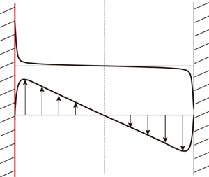
Figure 1. (a) Schematic of the VC in an infinite channel. (b) Illustration of the mean temperature and velocity profiles.

In channel VC, the mean velocity and temperature profiles have been a longstanding topic of research, garnering continued interest from 1979 to the present (George & Capp 1979; Versteegh & Nieuwstadt 1999; Hölling & Herwig 2005; Shiri & George 2008; Kiš & Herwig 2012; Ng et al. 2017; Howland et al. 2022). In the pioneering work by George & Capp (1979), the velocity and temperature fields are both divided into a viscous inner region near the wall, and a fully turbulent outer region near the channel centre. The outer region merges with the inner one at a certain zone that is usually called the overlap region (George & Capp 1979; Versteegh & Nieuwstadt 1999; Hölling & Herwig 2005; Shiri & George 2008; Ng et al. 2013). Based on a heuristic understanding of the flow in the inner region, where, for instance, the Prandtl number dependence must be retained since it appears in the normalised governing equations, the scaling analysis by George & Capp (1979) shows that the inner characteristic scales for temperature, velocity and length read $T_l=|F_0|^{3/4}(g \beta \alpha )^{-1/4}$, $U_l=( g\beta \,|F_0|\, \alpha )^{1/4}$ and $\eta =[ \alpha ^3/(g\beta \,|F_0|)]^{1/4}$, respectively. The product of the gravity acceleration and the thermal expansion coefficient $g\beta$, and the heat flux $F_0=\alpha \, \partial T/\partial y$, both represent the effect of the heated wall, and the thermal diffusivity $\alpha$ represents the effect of the Prandtl number. Similarly, with a heuristic understanding of the flow in the outer region, the outer characteristic scales can be also derived via the scaling analysis. Then the mean velocity and temperature profiles in both inner and outer regions are expressed in the form of abstract functions. By further assuming that the inner and outer abstract profiles are both valid in the overlap region, George & Capp (1979) eventually derived the profiles in power-law form for the overlap region, using the gradient-matching approach.

The mean temperature profile in the overlap region by George & Capp (1979) has been well confirmed by most studies, while the mean velocity profile is recognised to be problematic (Versteegh & Nieuwstadt 1999; Hölling & Herwig 2005; Shiri & George 2008). To solve this problem, guided by various heuristic understandings of channel VC, different characteristic scales have been proposed to normalise the inner and outer abstract profiles (Ng et al. 2013). For example, Hölling & Herwig (2005) found that the horizontal heat flux is a constant across the whole channel; thus they applied a single characteristic scale for temperature in both inner and outer regions, instead of two different ones as suggested by George & Capp (1979). These proposed characteristic scales have led to different mean profiles, which, however, still suffer from their own shortcomings. In the model of Versteegh & Nieuwstadt (1999), the shortcoming, as concluded by the authors themselves, is that the inner and outer velocity gradients do not match in the overlap region. In the model of Hölling & Herwig (2005), the involved coefficient in the mean temperature profile was found to be not constant by Kiš & Herwig (2012), indicating the lack of generality. To mitigate this, Kiš & Herwig (2012) introduced a probability density function to approximate this coefficient. As a result, a combination of a logarithmic function and an error function is proposed for the mean temperature profile. However, as the probability density function is entirely empirical, the derived mean temperature profile is still limited in its applicability. In the model of Shiri & George (2008), the mean velocity profile was developed theoretically as a log law, supposed to be valid across the full range of Rayleigh numbers in the turbulent regime; however, this log velocity profile was not recovered in the recent numerical studies by Ng et al. (2017) and Howland et al. (2022).

As indicated above, several analytical mean profiles have been proposed for the velocity and temperature in channel VC, but none of them is universally valid. Moreover, the recent numerical studies have also failed to reach a consensus on the form of mean profiles in channel VC: Ng et al. (2017) did not observe a log behaviour in either mean velocity or mean temperature profiles, while Howland et al. (2022) believed that their mean temperature profile exhibits a log behaviour. These indicate clearly that the mean profiles in channel VC are still rather debatable, and none of the existing profiles is general enough to predict data from different literatures in a unified manner. Such a problem could be attributed to the scaling analyses involved in the derivations, where the characteristic scales for velocity, temperature and length are proposed on the basis of various heuristic understandings, thus a sound mathematical description is generally not ensured. In addition, it should be pointed out that the reported mean profiles are all discussed and verified within the classical regime of turbulence, where the near-wall parts of the velocity and temperature boundary layers (BLs) are both laminar. As buoyancy gets extremely strong, the near-wall parts of the BLs would become turbulent, and channel VC will undergo a transition to the so-called ultimate regime of turbulence, in which both mean velocity and temperature profiles are expected to follow log laws, by analogy with the result in Rayleigh–Bénard convection (RBC) (Ng et al. 2017; Howland et al. 2022). However, as already highlighted in previous studies (Ng et al. 2015; Shishkina 2016), the flow dynamics between VC and RBC are not entirely identical, and this results in the fact that the Grossmann–Lohse theory, developed originally for RBC, cannot be applied directly to VC. Similarly, the non-identical flow dynamics may also bring some challenges to the straightforward profile analogy between VC and RBC systems. Thus it is necessary to provide a further discussion regarding the log-law expectation in the ultimate regime of channel VC.

In this study, the main objective is twofold: one objective is to develop mean profiles for velocity and temperature in channel VC that are universally valid, with the ability of interpreting data from different sources; the other is to shed some light on the profile analogy between VC and RBC systems in the ultimate regime. To these ends, the mean profiles are derived from the flow governing equations, with turbulent heat flux and Reynolds shear stress closed by the mixing length theory, in § 2. The validations and discussions are given in § 3. Finally, we conclude this paper in § 4.

2. Mean velocity and temperature profiles

As shown in figure 1(a), the VC system under consideration is confined in a channel consisting of two no-slip and impenetrable vertical walls, separated by a distance $H$. The two walls are kept at constant temperatures $T_h$ and $T_c$, respectively, with $T_h > T_c$. In the streamwise ($x$) and spanwise ($z$) directions, periodic boundary conditions are imposed for both velocity and temperature. Under this configuration, the temperature difference ${\rm \Delta} T=T_h-T_c$ would eventually establish a turbulent flow at sufficiently high $H$, and would result in antisymmetric mean velocity and temperature profiles with respect to the channel centre (figure 1b) (Versteegh & Nieuwstadt 1999; Hölling & Herwig 2005; Shiri & George 2008; Kiš & Herwig 2012; Ng et al. 2013, 2017; Howland et al. 2022; Ching 2023). Accordingly, all turbulence statistics of the velocity and temperature would depend only on the wall normal coordinate ($\kern 0.06em y$); thus the equations for the mean flow can be simplified as (George & Capp 1979; Versteegh & Nieuwstadt 1999; Hölling & Herwig 2005; Shiri & George 2008; Ng et al. 2013; Ching 2023)

(2.1a)$$\begin{gather} 0 =g\beta(\bar T-T_{{ref}})+\nu\,\frac{\partial^2 \bar u}{\partial y^2}- \frac{\partial \overline{u^\prime v^\prime}}{\partial y}, \end{gather}$$

(2.1b)$$\begin{gather}0 =\alpha\,\frac{\partial^2 \bar T}{\partial y^2}- \frac{\partial \overline{v^\prime T^\prime}}{\partial y}, \end{gather}$$

where the overbar and the prime respectively denote the mean and the fluctuating quantities. Specifically, the temperature field is denoted by $T$, and a reference temperature is defined as $T_{{ref}}=(T_h+T_c)/2$. The streamwise and normal components of the velocity are denoted as $u$ and $v$, respectively. All the fluid properties, including kinematic viscosity $\nu$ and thermal diffusivity $\alpha$, are considered to be constant. Meanwhile, the Boussinesq approximation is adopted, which implies that the temperature variation affects only the buoyancy. As a result, the present channel VC system is governed by the Rayleigh number ${Ra}=g\beta \,{\rm \Delta} T\,H^3/(\nu \alpha )$ and the Prandtl number ${Pr}=\nu /\alpha$.

The integration of (2.1a,b) from the hot wall to a certain wall-normal distance, i.e. over a range $[0,y]$, leads to

(2.2a)$$\begin{gather} \int_0^y g\beta(\bar T-T_{{ref}})\,{\rm d}\mathcal{Y}+\nu\,\frac{\partial \bar u}{\partial y}-\nu \left(\frac{\partial \bar u}{\partial y} \right)_w-\overline{u^\prime v^\prime}=0, \end{gather}$$

(2.2b)$$\begin{gather}\alpha\,\frac{\partial \bar T}{\partial y}-\overline{v^\prime T^\prime}=\alpha \left(\frac{\partial \bar T}{\partial y}\right)_w, \end{gather}$$

where the integration variable is denoted by $\mathcal {Y}$, and the subscript $w$ indicates the quantity at the hot wall ($\kern 0.06em y=0$). It should be noted that we have used $(\overline {u^\prime v^\prime })_w = 0$ and $(\overline {v^\prime T^\prime })_w = 0$ in the above integrations. In (2.2a,b), the wall shear stress and the wall heat flux are usually related to the friction velocity ($u_*$) and the friction temperature ($T_*$), respectively, as $\nu (\partial \bar u/\partial y)_w=u_*^2$ and $-\alpha (\partial \bar T/\partial y)_w/u_*=T_*$ (Kader & Yaglom 1972; Ng et al. 2017; Howland et al. 2022). In addition, the Reynolds shear stress and the turbulent heat flux are usually closed by the mixing length theory, which works well in modelling turbulent flows with a single characteristic length (Tennekes & Lumley 1972) and has been applied successfully to turbulent RBC systems with infinite horizontal extent (Grossmann & Lohse 2012; Shishkina et al. 2017). In the present channel VC, only one characteristic length, i.e. the distance $H$ between the two vertical walls, is involved. Thus the turbulent fluctuating terms in (2.2a,b) can be modelled effectively by the mixing length theory as $\overline {u^\prime v^\prime }=-k_1y^2 (\partial \bar u/\partial y)(\partial \bar u/\partial y)$ and $\overline {v^\prime T^\prime }=-k_2 y^2(\partial \bar u/\partial y) (\partial \bar T/\partial y)$, where $k_1$ and $k_2$ are dimensionless coefficients. With these relations, the integration equations (2.2a,b) become

(2.3a)$$\begin{gather} \int_0^y g\beta(\bar T-T_{{ref}})\,{\rm d}\mathcal{Y}+\nu\,\frac{\partial \bar u}{\partial y}-u_*^2+k_1 y^2\,\frac{\partial \bar u}{\partial y}\,\frac{\partial \bar u}{\partial y}=0, \end{gather}$$

(2.3b)$$\begin{gather}\alpha\,\frac{\partial \bar T}{\partial y}+k_2 y^2\,\frac{\partial \bar u}{\partial y}\,\frac{\partial \bar T}{\partial y}= - u_* T_*. \end{gather}$$

Further dividing (2.3a) by $u_*^2$ and (2.3b) by $-u_* T_*$, one obtains the dimensionless integration equations as

(2.4a)$$\begin{gather} \frac{\displaystyle\nu \int_0^{y_+} g\beta(\bar T-T_{{ref}})\,{\rm d}\mathcal{Y}_+}{u_*^3}+ \frac{\partial u_+}{\partial y_+}+k_1 y_+^2\,\frac{\partial u_+}{\partial y_+}\,\frac{\partial u_+}{\partial y_+}=1, \end{gather}$$

(2.4b)$$\begin{gather}\frac{\partial T_+}{\partial y_+}+k_2\,{Pr}\,y_+^2\,\frac{\partial u_+}{\partial y_+}\,\frac{\partial T_+}{\partial y_+}={Pr}, \end{gather}$$

where the mean velocity, the mean temperature and the wall-normal distance are naturally normalised as $u_+=\bar u/u_*$, $T_+=(T_h-\bar T)/T_*$ and $y_+=u_*y/\nu$, respectively. The above dimensionless integration equations (2.4a,b) are nonlinear and cannot be solved analytically. However, through appropriate simplifications, they will become solvable in certain regions of the channel, as presented below.

Near the hot wall ($\kern 0.06em y_+ \to 0$), one has $\nu \int _0^{y_+} g\beta (\bar T-T_{{ref}})\,{\rm d}\mathcal {Y}_+/u_*^3 \rightarrow 0$ and $k_1 y_+^2 (\partial u_+/\partial y_+)^2 \rightarrow 0$ in (2.4a), and $k_2\,{Pr}\,y_+^2 (\partial u_+/\partial y_+)(\partial T_+/\partial y_+) \rightarrow 0$ in (2.4b). Thus the dimensionless integration equations (2.4a,b) can be simplified as

(2.5a)$$\begin{gather} \frac{\partial u_+}{\partial y_+}=1, \end{gather}$$

(2.5b)$$\begin{gather}\frac{\partial T_+}{\partial y_+}={Pr}, \end{gather}$$

where only the molecular diffusion terms are retained. However, it is worth mentioning that the buoyancy term could also play a significant role in the near-wall region (at small $y_+$ values), as suggested numerically by Wei (2019). This would then lead to another set of simplified equations accounting for the buoyancy effect:

(2.6a)$$\begin{gather} \frac{\displaystyle\nu \int_0^{y_+} g\beta(\bar T-T_{{ref}})\,{\rm d}\mathcal{Y}_+}{u_*^3}+ \frac{\partial u_+}{\partial y_+}=1, \end{gather}$$

(2.6b)$$\begin{gather}\frac{\partial T_+}{\partial y_+}={Pr}. \end{gather}$$

Near the channel centre ($\kern 0.06em y_+ \rightarrow \infty$), one has $k_1 y_+^2 (\partial u_+/\partial y_+)^2 \gg \partial u_+/\partial y_+$ in (2.4a) and $k_2\,{Pr}\,y_+^2 (\partial u_+/\partial y_+)(\partial T_+/\partial y_+) \gg \partial T_+/\partial y_+$ in (2.4b). In this case, the dimensionless integration equations (2.4a,b) reduce to

(2.7a)$$\begin{gather} \frac{\displaystyle\nu \int_0^{y_+} g\beta(\bar T-T_{{ref}})\,{\rm d}\mathcal{Y}_+}{u_*^3}+k_1 y_+^2\, \frac{\partial u_+}{\partial y_+}\,\frac{\partial u_+}{\partial y_+}=1, \end{gather}$$

(2.7b)$$\begin{gather}k_2 y_+^2\,\frac{\partial u_+}{\partial y_+}\,\frac{\partial T_+}{\partial y_+}=1, \end{gather}$$

where only the buoyancy and the turbulent mixing terms are retained.

In the intermediate region between the wall and the channel centre (intermediate $y_+$), the dimensionless integration equations (2.4a,b) cannot be simplified, in which all molecular diffusion and turbulent mixing terms remain.

With no-slip velocity and constant temperature boundary conditions at the hot wall ($\kern 0.06em y_+=0$: $u_+=0$ and $T_+=0$), the integration of (2.5a,b), which excludes the buoyancy effect, yields the mean velocity and temperature profiles near the wall as

(2.8a)$$\begin{gather} u_+ = y_+, \end{gather}$$

(2.8b)$$\begin{gather}T_+ = {Pr}\,y_+, \end{gather}$$

which are linear and recover the numerical observations of Ng et al. (2017) and Howland et al. (2022). If we take the buoyancy effect into account, then the mean profiles near the wall are obtained via the integration of (2.6a,b) as

(2.9a)$$\begin{gather} u_+ = y_+ - \frac{1}{4}\,\frac{\nu g\beta T_*}{u_*^3}\,\frac{{\rm \Delta} T}{T_*}\,y_+^2+\frac{Pr}{6}\, \frac{\nu g\beta T_*}{u_*^3}\,y_+^3, \end{gather}$$

(2.9b)$$\begin{gather}T_+ = {Pr}\,y_+, \end{gather}$$

where the cubic velocity profile is deduced by substituting (2.9b) into (2.6a), and it is consistent with the reported profiles in the previous studies (Tsuji & Nagano 1988a; Hölling & Herwig 2005; Ke et al. 2020, 2021). The cubic velocity profile includes the buoyancy effect, thus it is expected to show a wider applied range compared with the linear one, which is applicable only at $y_+ \to 0$. Nevertheless, this does not imply that there is a significant difference between the two velocity profiles. In fact, the cubic velocity profile is compatible with and can reduce to the linear one, since at $y_+ \to 0$, the quadratic and cubic correction terms in (2.9a) would become negligible relative to the linear term. In addition, although the linear velocity profile can be regarded as a reduced case of the cubic one, it is indispensable in understanding channel VC. This is because the linear velocity profile is a solid signature of the constant stress layer.

In the following, we derive the mean velocity and temperature profiles near the channel centre. Differentiating (2.7a) twice with respect to $y_+$, one obtains

(2.10)\begin{equation} -\!\frac{\nu g\beta T_*}{u_*^3}\,\frac{\partial T_+}{\partial y_+}+ \frac{\partial^2}{\partial y_+^2}\left(k_1 y_+^2\,\frac{\partial u_+}{\partial y_+}\, \frac{\partial u_+}{\partial y_+} \right)=0. \end{equation}

Substituting the temperature gradient ${\partial T_+}/{\partial y_+}$ obtained from the above equation into (2.7b), one has

(2.11)\begin{equation} y_+^2\,\frac{\partial u_+}{\partial y_+}\,\frac{\partial^2}{\partial y_+^2} \left(y_+^2\,\frac{\partial u_+}{\partial y_+}\,\frac{\partial u_+}{\partial y_+} \right)= \frac{\nu g\beta T_*}{u_*^3 k_2 k_1}. \end{equation}

This equation is nonlinear and cannot be solved via direct integrations. Nevertheless, it is noticed that the right-hand side of (2.11) is a constant, which thereby requires that the left-hand side must be independent of $y_+$. To meet this requirement, the velocity gradient must take the form $\partial u_+/\partial y_+=ky_+^\gamma$, with which (2.11) can be rewritten as

(2.12)\begin{equation} k^3 (2\gamma+2)(2\gamma+1)y_+^{3\gamma+2}=\frac{\nu g\beta T_*}{u_*^3 k_2 k_1}. \end{equation}

Further, the requirement of $y_+$ independence results in $\gamma =-2/3$ and $k=[-9\nu g \beta T_*/(2u_*^3 k_2 k_1)]^{1/3}$. Then the velocity and temperature gradients can be expressed as

(2.13a)$$\begin{gather} \frac{\partial u_+}{\partial y_+}=\left(-\frac{9\nu g \beta T_*}{2u_*^3k_2 k_1} \right)^{1/3} y_+^{ - 2/3}, \end{gather}$$

(2.13b)$$\begin{gather}\frac{\partial T_+}{\partial y_+}=\frac{1}{k_2} \left(-\frac{9\nu g \beta T_*}{2u_*^3k_2 k_1} \right)^{ - 1/3} y_+^{ - 4/3}, \end{gather}$$

where the temperature gradient is obtained by substituting (2.13a) into (2.7b). Integrating these gradients would provide us with the mean velocity and temperature profiles, and the corresponding integration constants are determined by the antisymmetry of the mean fields (figure 1b), namely at $y_+=u_*H/(2\nu )$: $u_+=0$ and $T_+={\rm \Delta} T/(2T_*)$. Consequently, the mean velocity and temperature profiles near the channel centre are

(2.14a)$$\begin{gather} u_+ = c_1\big[\left(\mathcal{K}y_+ \right)^{1/3}-\mathcal{K}_0^{1/3} \big], \end{gather}$$

(2.14b)$$\begin{gather}T_+ = c_2\big[\left(\mathcal{K}y_+ \right)^{ - 1/3}-\mathcal{K}_0^{ - 1/3} \big]+\frac{{\rm \Delta} T}{2T_*}, \end{gather}$$

where $\mathcal {K}=\nu g\beta T_*/u_*^3$, $\mathcal {K}_0=g\beta T_*H/(2u_*^2)$, $c_1=-3[9/(2k_2k_1)]^{1/3}$ and $c_2=3k_2^{-1} [9/(2k_2k_1)]^{-1/3}$. Recalling $\nu (\partial \bar u/\partial y)_w=u_*^2$ and $-\alpha (\partial \bar T/\partial y)_w/u_*=T_*$, it is seen that $\mathcal {K}$ and $\mathcal {K}_0$ actually depend on $Pr$, indicating that the fluid property would influence the mean profiles, similar to the situation in RBC systems (Grossmann & Lohse 2012).

To sum up, this section develops the mean profiles in the region near the wall ($\kern 0.06em y_+ \to 0$) and that near the channel centre ($\kern 0.06em y_+ \to \infty$), where the mean flow is dominated by the molecular diffusion (2.5a,b) and the turbulent mixing (2.7a,b), respectively. For convenience, these two regions are respectively referred to as the ‘viscosity-dominated sublayer’ and ‘turbulence-dominated sublayer’ in the subsequent discussions. Accordingly, the region connecting these two sublayers is referred to as the intermediate sublayer. The intermediate sublayer encompasses the effects of both molecular diffusion and turbulent mixing, and its role is the same as that of the buffer sublayer in RBC systems (Ahlers, Bodenschatz & He 2014) and wall shear flows (Pope 2000). Thus the mean profiles in the intermediate sublayer would smoothly connect those in the viscosity-dominated sublayer and those in the turbulence-dominated sublayer, but they cannot be derived analytically by simplifying the governing equations (2.4a,b). In addition, as the turbulent level increases, the intermediate sublayer will be squeezed gradually by the turbulence-dominated sublayer, and eventually vanishes, as will be discussed in the next section. Thus although the mean profiles in the intermediate sublayer are not modelled, it will not cause a severe problem in vigorous turbulent channel VC. In fact, in well-discussed RBC systems, the mean profiles in the intermediate (buffer) sublayer have not been examined either (Ahlers et al. 2014).

3. Validations and discussions

In this section, we first validate the present profiles in (2.8a,b), (2.9a,b) and (2.14a,b) by comparing them with data available in the literature, in a parameter space $5.4\times 10^5 \leq {Ra} \leq 10^9$ and $0.709\leq {Pr} \leq 100$, which corresponds to the classical regime of turbulence. Then the present profiles are compared with those reported in literature, also in the classical regime. The final subsection is dedicated to the discussion of the profile analogy between VC and RBC systems in the ultimate regime of turbulence.

3.1. Validations

The literature data for the verification of the present profiles include those from Versteegh & Nieuwstadt (1999), Ng et al. (2017) and Howland et al. (2022), where the data set by Versteegh & Nieuwstadt (1999) has been used widely as the benchmark in many studies (Hölling & Herwig 2005; Pallares et al. 2010; Ng et al. 2013), and Ng et al. (2017) and Howland et al. (2022) present the latest numerical data in channel VC. In figure 2, we compare the present profiles with the data collected from the literature. It is seen clearly that all the data show a linear relationship for $u_+$ ($\kern 0.06em y_+$) and $T_+$ ($\kern 0.06em y_+$) near the hot wall (figures 2a,b), consistent with the predictions in (2.8a,b). Meanwhile, with $(\mathcal {K} y_+)^{1/3}-\mathcal {K}_0^{1/3}$ and $(\mathcal {K} y_+)^{-1/3}-\mathcal {K}_0^{-1/3}$ being the horizontal axes, these data collapse into straight lines close to the channel centre (figures 2c,d), as predicted by the power profiles (2.14a,b). From figures 2(c,d), one could further obtain the unknown coefficients $c_1$ and $c_2$ in (2.14a,b) via linear fittings as

(3.1a,b)\begin{equation} c_1 \approx - 10.0 \quad {\rm and} \quad c_2 \approx - 3.8. \end{equation}

To illustrate the universality of the fitted $c_1$ and $c_2$, more data from Howland et al. (2022) are employed for further comparisons (figure 3). It is worth emphasising that the data presented in figure 3 are produced at rather different ${Ra}$ from those in figure 2. Additionally, as a direct indicator of the turbulence level, the corresponding values of the Reynolds number ($Re$) are also indicated in figure 3, which are estimated from the scaling correlation developed by Howland et al. (2022):

(3.2)\begin{equation} {Re}=\frac{u_* H}{\nu} \sim {Ra}^{0.362}\,{Pr}^{ - 0.446}. \end{equation}

It is clear in figure 3 that the applied range of the cubic velocity profile (2.9a) is expanded greatly compared with the linear one (2.8a), as expected. Moreover, the power mean profiles (2.14a,b), computed with the fitted values of $c_1$ and $c_2$ (3.1a,b), agree well with the literature data in the vicinity of the channel centre. At the same time, figure 3 also indicates that away from the channel centre, the applied range for the power mean profiles and the fitted coefficients diminishes gradually with decreasing Reynolds number, eventually becoming insignificant at very low $Re$. This behaviour is entirely expected and does not suggest any issues with the present profiles or fitted coefficients, since the power profiles arise from turbulent mixing, and naturally their applied range will diminish as the turbulence level (the value of ${Re}$) decreases. Similar behaviour has also been observed in wall shear flows, where the applied range for the well-known log velocity profile and the von Kármán constant (typically approximately 0.4) also diminishes with decreasing ${Re}$, eventually vanishing at very low ${Re}$, such as those indicative of a laminar state (Kundu, Cohen & Dowling 2012, p. 586). Nevertheless, it is widely recognised that the log velocity profile and its von Kármán constant are universal in wall shear flows. Likewise, the present power profiles and the corresponding fitted coefficients can also be deemed as universal in channel VC, as they describe effectively all available literature data, except for cases at very low ${Re}\leq 109.1$, as shown in figure 3 and in the next subsection.

Figure 2. Comparisons between the present profiles (red lines) and the literature data (discrete symbols) (Versteegh & Nieuwstadt 1999; Ng et al. 2017; Howland et al. 2022). (a,b) Mean velocity and temperature profiles near the wall (2.8a,b). (c,d) Mean velocity and temperature profiles near the channel centre (2.14a,b).

Figure 3. Three-sublayer structure of the mean fields in channel VC. The orange and blue backgrounds denote the viscosity-dominated and the turbulence-dominated sublayers respectively, where the prediction relative error of the present mean profiles is less than $10\,\%$. The grey background represents the intermediate sublayer that connects smoothly the two aforementioned sublayers. Only the results in the left half of the channel are illustrated, and those in the right half can be obtained according to the antisymmetry of the mean fields. All the discrete data points (black squares) presented in this figure are from Howland et al. (2022). Also note that the horizontal axis is in log scale.

In order to further quantify the effect of ${Re}$, we introduce a relative error ($E$) defined as

(3.3a,b)\begin{equation} {E_u}=\frac{|u_{{pre}}-u_{{rep}}|}{u_{{rep}}}\quad {\rm and}\quad {E_T}=\frac{|T_{{pre}}-T_{{rep}}|}{T_{{rep}}}, \end{equation}

where the subscripts ‘$pre$’ and ‘$rep$’ refer to the predicted mean profiles and the corresponding reported data in the literature, respectively. With this definition, we restrict the viscosity-dominated velocity and temperature sublayers to regions $E_u \leq 10\,\%$ and $E_T \leq 10\,\%$, when $u_{{pre}}$ and $T_{{pre}}$ are calculated from the viscous-form profiles (2.9a,b). The procedure for identifying the turbulence-dominated velocity and temperature sublayers is analogous, with the only difference being that $u_{{pre}}$ and $T_{{pre}}$ are calculated from the turbulent-form profiles (2.14a,b). In this way, the applied range of the viscous-form profiles and that of the turbulent-form profiles can be represented by the widths ($W$) of viscosity-dominated and turbulence-dominated sublayers, respectively. These widths are further normalised by the channel width ($H$), and reflect the space occupancy (${SO}$) of each sublayer:

(3.4a,b)\begin{equation} {SO_u}=\frac{2 W_u}{H}\quad {\rm and}\quad {SO_T}=\frac{2 W_T}{H}, \end{equation}

where the subscripts $u$ and $T$ denote the sublayers of the velocity BL and those of the temperature BL, respectively. The prefactor 2 is due to the fact that each sublayer appears not only in the left half of the channel, but also in the right half. Obviously, the space occupancy of each sublayer is a dimensionless quantity that measures the applied range of the profile within that sublayer.

The space occupancy of each sublayer shown in figure 3 is calculated, and presented as a function of the Reynolds number in figure 4. Clearly, it provides a confirmation that the space occupancy of the turbulence-dominated sublayer, representing the applied range of the power profiles, increases with increasing $Re$. Thus the narrow applied range of the power profiles observed at low $Re \sim 43.9$ (figures 3i,l) is an expected consequence.

Figure 4. Space occupancy for the three sublayers of (a) mean velocity and (b) mean temperature. The data here are from figures 3 and 5. It is important to note that the space occupancy of each sublayer also represents the dimensionless applied range for the profile within that sublayer.

In figure 4, other results are suggested as well. First, as ${Re}$ increases to a sufficiently high value, the space occupancy of the turbulence-dominated sublayer will be approaching unity, meaning that this sublayer will eventually occupy the entire channel. In other words, channel VC will be entirely turbulent, being consistent with the expectation for the ultimate regime. Second, as the turbulence-dominated sublayer extends, the intermediate sublayer will be squeezed gradually until vanishing, indicating that this sublayer is an impermanent structure without fixed boundaries. Finally, although the space occupancies of the power profiles are visually limited close to the channel centre (e.g. figure 3h), they are much larger than they look since the horizontal axis is in log scale. In fact, following the criterion $E \leq 10\,\%$, it is found that when ${Re}>122$, the predicted region of the velocity power profile extends beyond $30\,\%$ of the channel, and that of the temperature power profile extends beyond $80\,\%$ of the channel, as illustrated in figure 4. This demonstrates the validity of the present mean profiles.

In addition, it is noticed that the temperature power profiles present a much wider applied range than the velocity power profiles in figure 4. This is actually a natural outcome, and can be understood in the following way. Although the power profiles for velocity and temperature both arise from turbulent mixing, the scalars transferred via turbulent mixing are different. Specifically, the velocity power profile results from the mixing of kinetic energy, thus its applied range depends on the turbulent viscosity $\nu _t$, which measures the mixing intensity of kinetic energy. By contrast, the temperature power profile originates from the mixing of heat, thus its applied range depends on the turbulent thermal diffusivity $\alpha _t$, which measures the mixing intensity of heat. Consequently, the ratio of applied range of the velocity power profile to the temperature power profile reads

(3.5)\begin{equation} \frac{\text{applied range of velocity power profile}}{\text{applied range of temperature power profile}}\propto \frac{\nu_t}{\alpha_t}= {Pr}_t, \end{equation}

where ${Pr}_t$ is the turbulent Prandtl number and has been investigated thoroughly by Jischa & Rieke (1979), who concluded that ${Pr}_t<1$ for ${Pr}\gtrsim 1$. Later, Hölling & Herwig (2005) found ${Pr}_t \approx 0.9$ numerically at ${Pr} =0.709$. Thus in the parameter space considered in this study ($100 \geq {Pr} \geq 0.709$), ${Pr}_t$ should be less than 1, indicating that the applied range of the velocity power profile should be lower than that of the temperature power profile (3.5). This explains why it is much more difficult for the space occupancy of the velocity turbulence-dominated sublayer to approach unity as ${Re}$ increases, compared with the temperature turbulence-dominated sublayer (figures 4a,b). Finally, it should be pointed out that different applied ranges for the velocity and temperature power profiles are not in contradiction with the derivations, where the mean velocity and temperature profiles are derived simultaneously at the channel centre ($\kern 0.06em y_+ \to \infty$) only (see (2.7a,b)). This requires that the upper bounds of these applied ranges must be overlapping at the channel centre, but does not require the lower bounds to be the same, indicating that the two applied ranges can be different.

3.2. Comparisons with the reported profiles in the classical regime

In the previous studies, considerable efforts have been devoted to determining the mean profiles, and a consensus has been reached in the near-wall region, where the mean profiles follow linear laws (2.8a,b). As stated before, the cubic velocity profile (2.9a) will reduce to the linear one (2.8a) at $y_+ \to 0$. However, the reported mean profiles in the region at a distance from the wall are rather debatable, which in the pioneer work of George & Capp (1979) reads

(3.6a)$$\begin{gather} \frac{\bar{u}}{U_l}=\phi_1\left(\frac{y}{\eta} \right)^{1/3}+A({Pr}), \end{gather}$$

(3.6b)$$\begin{gather}\frac{T_h-\bar{T}}{T_l}= - \phi_2\left(\frac{y}{\eta} \right)^{ - 1/3}-B({Pr}), \end{gather}$$

where $\phi _1$ and $\phi _2$ are dimensionless coefficients, and $A({Pr})$ and $B({Pr})$ are unknown functions of the Prandtl number. By incorporating $T_l=|F_0|^{3/4}(g \beta \alpha )^{-1/4}$, $U_l=( g\beta \,|F_0|\,\alpha )^{1/4}$ and $\eta =[ \alpha ^3/(g\beta \,|F_0|)]^{1/4}$, these profiles are transformed into

(3.7a)$$\begin{gather} u_+ = \phi_1\left(\mathcal{K}y_+ \right)^{1/3}+A({Pr})\,(\alpha g \beta T_*/u_*^3)^{1/4}, \end{gather}$$

(3.7b)$$\begin{gather}T_+ = -\phi_2\left(\mathcal{K}y_+ \right)^{ - 1/3}-B({Pr})\,(\alpha g \beta T_*/u_*^3)^{ - 1/4}. \end{gather}$$

These results were developed originally for plate VC, and they were applied to channel VC by subsequent studies (Versteegh & Nieuwstadt 1999; Ng et al. 2013). In these studies, the mean temperature profile has been well confirmed, and the dimensionless coefficients were fitted as $\phi _2=4.2$ and $B=-5.0$ when ${Pr}=0.709$ (Versteegh & Nieuwstadt 1999; Ng et al. 2013), while the mean velocity profile was found to be problematic, and no fitted values for $\phi _1$ and $A({Pr})$ were documented. As a result, Versteegh & Nieuwstadt (1999) proposed a modified linear velocity profile

(3.8)\begin{equation} u_+ = y_+ - \frac{U_l}{u_*}\,\frac{9.7(y/\eta)^2}{2.8+y/\eta}, \end{equation}

and Shiri & George (2008) proposed a log velocity profile

(3.9)\begin{equation} u_+ = \mathcal{P}\ln(y_+)+\mathcal{Q}({Pr}). \end{equation}

However, this log profile was not compared with any numerical or experimental data, and the fitted coefficients of $\mathcal {P}$ and $\mathcal {Q}({Pr})$ were not provided either. Then Hölling & Herwig (2005) proposed another set of mean profiles:

(3.10a)\begin{align} u_{{\times}}&=\frac{0.427\,{Pr}}{0.9}\,y_{{\times}} \left[ 0.427(\ln y_{{\times}}-2)+1.93-T_{{\times} 0}\right] \nonumber\\ &\quad +\left[0.49 \left(\frac{\partial u_{{\times}}}{\partial y_{{\times}}}\right)_w -2.27\right]\ln y_{{\times}}+1.28\left(\frac{\partial u_{{\times}}}{\partial y_{{\times}}}\right)_w+1.28, \end{align}

(3.10b)\begin{align} &T_{{\times}}=0.427\ln y_{{\times}}+1.93, \end{align}

where the dimensionless variables are

(3.11) \begin{equation} \left\{\begin{array}{l} y_{{\times}}=y_+({Pr}^3 \mathcal{K})^{1/4},\\ T_{{\times}}=T_+\left(\dfrac{\mathcal{K}}{Pr}\right)^{1/4},\\ T_{{\times} 0}=0.5\,{\rm \Delta} T \left(\dfrac{g\beta \alpha}{u_*^3T_*^3}\right)^{1/4},\\ u_{{\times}}=u_+ \left(\dfrac{{Pr}^5}{\mathcal{K}}\right)^{1/4},\\ \left(\dfrac{\partial u_{{\times}}}{\partial y_{{\times}}}\right)_w= \left(\dfrac{\partial u_{+}}{\partial y_{+}}\right)_w \left(\dfrac{Pr}{\mathcal{K}}\right)^{1/2}. \end{array}\right. \end{equation}

However, a subsequent study by Kiš & Herwig (2012) pointed out that the constant coefficient 0.427 in (3.10b) was problematic and should be replaced by a probability density function. As a result, the log profile was modified as (Kiš & Herwig 2012)

(3.12)\begin{equation} T_{{\times}}=0.5+\ln(2y_{{\times}})+\mathcal{G}(y_\times)-\mathcal{G}(0.5), \end{equation}

with

(3.13)\begin{equation} \mathcal{G}(y_\times)=\frac{0.8}{0.877}\,\frac{\sqrt{\rm \pi}}{2}\,{\rm erf}[0.877(\ln y_{{\times}}-0.64)]. \end{equation}

These reported profiles are compared with the present profiles in figure 5. It is evident that the present mean profiles are the only ones that are able to interpret data from different literatures, thus demonstrating much better versatility compared with the reported ones. The improved versatility originates from the fact that the characteristic scales for velocity, temperature and length in the present profiles come naturally from the normalisation of the governing equations (2.4a,b), thus they possess a more sound mathematical basis than the previous characteristic scales obtained from various heuristic understandings of channel VC.

Figure 5. Mean profiles from the present study and those reported in the previous studies (George & Capp 1979; Versteegh & Nieuwstadt 1999; Hölling & Herwig 2005; Kiš & Herwig 2012) in channel VC. The discrete data are from (a,d) Ng et al. (2017) and (b,c,e, f) Howland et al. (2022). The orange and blue backgrounds denote the viscosity-dominated and turbulence-dominated sublayers, respectively, where the prediction relative error of the present mean profiles is less than $10\,\%$. The grey background represents the intermediate sublayer that connects smoothly the two aforementioned sublayers. Only the results in the left half of the channel are illustrated, and those in the right half can be obtained according to the antisymmetry of the mean fields. Also note that the horizontal axis is in log scale.

Further, figures 5(a–c) show that the mean velocity profiles can be described fully by the cubic law (prior to the maximum velocity) and the present $1/3$ power law (subsequent to the maximum velocity), except the intermediate sublayer enclosing the velocity peak. Obviously, this sublayer cannot be described by the log law. In addition, although a log law (3.9) is proposed for the mean velocity by Shiri & George (2008), this was not verified. Moreover, recent numerical studies by Ng et al. (2017) and Howland et al. (2022) have also failed to observe the log law behaviour in the classical regime. Thus it is reasonable to conclude that in the classical regime of turbulence, the mean velocity profile is unlikely to be logarithmic in channel VC.

Similarly, figures 5(d–f) show that the mean temperature profiles can be described fully by the linear law (prior to the maximum velocity) and the present $-1/3$ power law (subsequent to the maximum velocity), except the intermediate sublayer. This sublayer will finally vanish at sufficiently high ${Re}$ (figure 4b), and obviously cannot be described by the log law. In addition, although the log law (3.10b) was proposed for the mean temperature by Hölling & Herwig (2005), it can be applied only to certain parameters (figure 5d). Moreover, even at the certain parameter (figure 5d), the log law (3.10b) exhibits only a narrower agreement range, compared with the present $-1/3$ power profile. Thus it is reasonable to conclude that in the classical regime of turbulence, the mean temperature profile in channel VC is unlikely to be logarithmic as well.

In summary, in the classical regime of channel VC, the mean velocity and temperature profiles should not conform to log laws, in the region before, around or after the velocity peak. As for the ultimate regime in channel VC, there are still no literature data available to confirm the form of mean profiles, since the corresponding Rayleigh number needs to be extremely high and exceeds the critical value ${Ra}_c=4.27\times 10^{11}\times {Pr}^{1.89}$ (Howland et al. 2022). This correlation provides ${Ra}_c=2.2\times 10^{11}$ at ${Pr}=0.709$, aligning with the expectation of Ng et al. (2017), in which it is suggested that the ultimate regime in channel VC should occur at ${Ra} \gtrsim 10^{11}$ for the same Prandtl number.

3.3. Mean profiles in the ultimate regime

In the ultimate regime of turbulence, the mean profiles are assumed to follow log laws in channel VC, by analogy with RBC systems (Ng et al. 2017; Howland et al. 2022). Herein, we find that this assumption could encounter some challenges, and that the form of mean profiles in the ultimate regime may still follow power laws. Below, we present discussions regarding the form of mean profiles in the ultimate regime. It is important to emphasise that the discussions in this subsection are based merely on theoretical arguments, and there are not yet reported data or direct evidence to eventually judge the form of the mean profiles in the ultimate regime. Consequently, these envisioned power-law or log-law forms in the ultimate regime badly need further numerical or experimental confirmation in the future.

On the one hand, in fully developed turbulent channel VC, the turbulence statistics of the velocity and temperature would not vary along streamwise and spanwise directions, but depend on the normal coordinate only. Consequently, the equations of the mean flow will remain identical in both classical and ultimate regimes, resulting in the same laws for the mean profiles. In other words, once channel VC is in a fully developed turbulent state, the form of the mean profiles will not be altered by increasing ${Re}$. This implies that the linear, cubic and power laws derived in the classical regime may be still valid in the ultimate regime, and that increasing $Re$, i.e. the transition of classical–ultimate regimes, will not bring a new log profile. In fact, the ${Re}$-independent profile form has been confirmed in turbulent RBC systems with infinite horizontal extent (abbreviated as ‘channel RBC’ hereafter) in previous studies (Grossmann & Lohse 2012; Ahlers et al. 2014). It is found that in channel RBC, the mean temperature profile always follows a linear law close to the wall and a log law at a distance from the wall, and the transition of classical–ultimate regimes does not introduce any new profile (Grossmann & Lohse 2012; Ahlers et al. 2014). In addition, in turbulent wall shear flows, increasing ${Re}$ continuously will not bring any new form of profile either, and the well-known linear law near the wall and the log law away from the wall always hold.

On the other hand, in the ultimate regime, the velocity and temperature BLs are fully turbulent. This indicates that in this regime, both the viscosity-dominated and intermediate sublayers will be completely squeezed out by the turbulence-dominated sublayer. Thus if the log law is observed in the ultimate regime of channel VC, then it could appear only in the turbulence-dominated sublayer. In channel RBC, the log-law profile was indeed proposed in the turbulence-dominated sublayer (Grossmann & Lohse 2012; Ahlers et al. 2014). Since the turbulence-dominated sublayer is the only possible region to host the log-law profile, channel VC and channel RBC must then share the same flow equations in this sublayer, to ensure the validity of the profile analogy. In this sublayer, the equations of the mean flow in channel VC are given in (2.7a,b). In channel RBC, the equations governing the mean flow are derived as follows.

Consider a channel RBC system, with the horizontal (streamwise) and vertical (wall-normal) directions denoted by $x$ and $y$, respectively, and the fluid pressure denoted by $p$. After the system reaches the fully developed turbulent state, the mean velocity and temperature vary only along the vertical direction, thus the corresponding governing equations reduce to

(3.14a)$$\begin{gather} 0=\nu\,\frac{\partial^2 \bar u}{\partial y^2}-\frac{1}{\rho}\,\frac{\partial \bar p}{\partial x}-\frac{\partial \overline{u^\prime v^\prime}}{\partial y}, \end{gather}$$

(3.14b)$$\begin{gather}0= - \frac{1}{\rho}\,\frac{\partial \bar p}{\partial y}+g\beta(\bar T-T_{{ref}}), \end{gather}$$

(3.14c)$$\begin{gather}0=\alpha\,\frac{\partial^2 \bar T}{\partial y^2}-\frac{\partial \overline{v^\prime T^\prime}}{\partial y}. \end{gather}$$

Differentiating (3.14b) with respect to $x$, the buoyancy term $g\beta (\bar T-T_{{ref}})$ disappears because the mean temperature field $\bar {T}$ depends only on $y$. Consequently, one gets

(3.15)\begin{equation} \frac{\partial^2 \bar{p}}{\partial x\,\partial y}=0, \end{equation}

which indicates that the streamwise pressure gradient $\partial \bar {p}/\partial x$ stays the same along the normal direction, thus it can be estimated at the outside of the velocity BL. Beyond the velocity BL, the viscous effect becomes less important, and the corresponding streamwise pressure gradient can be modelled by Bernoulli's equation (Shishkina, Horn & Wagner 2013) as

(3.16)\begin{equation} \frac{\partial \bar{p}}{\partial x}= - \frac{\partial \rho \bar{u}^2(y)/2}{\partial x}=0. \end{equation}

Then the equations of the mean flow (3.14a–c) can be simplified further into

(3.17a)$$\begin{gather} 0=\nu\,\frac{\partial^2 \bar u}{\partial y^2}-\frac{\partial \overline{u^\prime v^\prime}}{\partial y}, \end{gather}$$

(3.17b)$$\begin{gather}0=\alpha\,\frac{\partial^2 \bar T}{\partial y^2}-\frac{\partial \overline{v^\prime T^\prime}}{\partial y}. \end{gather}$$

Following the same procedure as the derivations (2.1)–(2.4) for channel VC, the dimensionless integration equations resulting from (3.17a,b) read

(3.18a)$$\begin{gather} \frac{\partial u_+}{\partial y_+}+k_1 y_+^2\,\frac{\partial u_+}{\partial y_+}\,\frac{\partial u_+}{\partial y_+}=1, \end{gather}$$

(3.18b)$$\begin{gather}\frac{\partial T_+}{\partial y_+}+k_2\,{Pr}\,y_+^2\,\frac{\partial u_+}{\partial y_+}\,\frac{\partial T_+}{\partial y_+}={Pr}. \end{gather}$$

These equations in the turbulence-dominated sublayer ($\kern 0.06em y_+ \to \infty$) reduce to

(3.19a)$$\begin{gather} k_1 y_+^2\,\frac{\partial u_+}{\partial y_+}\,\frac{\partial u_+}{\partial y_+}=1, \end{gather}$$

(3.19b)$$\begin{gather}k_2 y_+^2\,\frac{\partial u_+}{\partial y_+}\,\frac{\partial T_+}{\partial y_+}=1. \end{gather}$$

Obviously, in the turbulence-dominated sublayer, the equations of the mean flow in channel VC (2.7a,b) are different from those in channel RBC (3.19a,b). Thus it is unlikely that the log profiles, which appear in channel RBC, will also manifest in channel VC. By comparison, the difference between the power profiles in channel VC and the log profiles in channel RBC arises from the buoyancy effect. In channel VC, the buoyancy is parallel to the mean flow, thus the buoyancy term should be included in the streamwise momentum equation (2.7a). This then results in the mean gradients $\partial u_+/ \partial y_+ \sim y_+ ^{-2/3}$ and $\partial T_+ /\partial y_+ \sim y_+ ^{-4/3}$ (2.13a,b), further leading to power profiles. By contrast, in channel RBC, the buoyancy is perpendicular to the mean flow, thus the buoyancy term is absent from the streamwise momentum equation (3.19a). Accordingly, the mean gradients become $\partial u_+/ \partial y_+ \sim y_+ ^{-1}$ and $\partial T_+/ \partial y_+ \sim y_+ ^{-1}$, and eventually result in the log profiles, recovering the results derived from a single mean temperature equation (Grossmann & Lohse 2012; Ahlers et al. 2014). In summary, in the turbulence-dominated sublayer where the log profile could be possible, although the mean temperature equations are the same in channel VC and channel RBC, (2.7b) and (3.19b), the streamwise momentum equations are quite different due to the buoyancy effect, (2.7a) and (3.19a). As a result, the log profiles in channel RBC may not be extended directly to channel VC in the ultimate regime by analogy.

4. Concluding remarks

This study focuses on the mean velocity and temperature profiles in fully developed turbulent channel VC. Instead of the conventional inner and outer two-region description, we employ a three-sublayer structure to depict both velocity and temperature fields, including the viscosity-dominated, intermediate and turbulence-dominated sublayers in turn from the wall to the channel centre. Within this framework, analytical expressions for the mean velocity and temperature profiles are developed in the viscosity- and turbulence-dominated sublayers. In the derivations, the mixing length theory is employed to close the turbulent mixing terms (2.3a,b), and it does not impose any restrictions on the results. Thus the derived mean profiles are expected to be valid over the full ranges of ${Ra}$ and ${Pr}$ in the turbulent state. This has been well confirmed by the reported data in the literature (figures 3 and 5), demonstrating that the present profiles make a significant improvement in versatility comparing with the reported ones, which are applicable only to certain parameter space (figure 5). Moreover, it is found that the applied range of the present power profiles increases as the Reynolds number rises (figure 4). Thus it is expected that these power profiles can describe the complete velocity and temperature distributions in channel VC as long as the turbulence becomes sufficiently vigorous. At present, the data for the most vigorous turbulent case from Ng et al. (2017) (figures 5a,d) have demonstrated that the present velocity power profile can predict $63.2\,\%$ of the channel, and the present temperature power profile can predict $99.4\,\%$ of the channel, with relative error no more than $10\,\%$. In addition, the turbulent Prandtl number is introduced to compare quantitatively the applied range of the velocity power profile and that of the temperature power profile (3.5).

Furthermore, the mean profiles in the ultimate regime of turbulence are discussed. We provide an analytical argument showing that the mean profiles of channel VC in the ultimate regime may remain in power laws, and the profile analogy between channel RBC and channel VC might need further consideration, since the flow dynamics is different between these two thermal flows. The main difference arises from the effect of buoyancy, which appears in the streamwise momentum transport of channel VC but is absent from that of channel RBC. However, it is essential to emphasise that the discussion regarding the power-law and log-law profiles envisioned in the ultimate regime is based merely on analytical arguments. A solid confirmation of the profile form in the ultimate regime still requires numerical or experimental data in the future. Additionally, we would like to point out that the present mean profiles are verified directly only for ${Pr}\geq 0.709$ via the data available in the literature. For the cases ${Pr}\ll 1$ (e.g. ${Pr} = 0.01$), there are no reported data available in channel VC yet, and the corresponding verification is not performed in this study. In spite of this, the present mean profiles are highly expected to be valid at low values of ${Pr}$, since they have incorporated the effect of ${Pr}$ without any assumptions, (2.9a,b) and (2.14a,b), and they have exhibited the ability to reconcile data at different ${Pr}$ in more than two decades (figure 5).

Finally, it is necessary to note that the present profiles are applicable to channel VC. In cavity VC, the mean convection terms in the governing equations are kept due to the effects of horizontal adiabatic walls, thus deserving further investigation. In plate VC, the mean flow also has exclusive dependence on the wall-normal coordinate; yet at the same time, this mean flow would consistently entrain the ambient fluid, leading to a streamwise-growing flow region. Consequently, the mean profiles no longer exhibit the antisymmetric characteristic, making them distinct from those in channel VC.