Analytic solution for pulse wave propagation in flexible tubes with application to a patient-specific arterial tree

Abstract

In this paper, we present an analytic solution for pulse wave propagation in a flexible arterial model with tapering, physiological boundary conditions and variable wall properties (wall elasticity and thickness). The change of wall properties follows a profile that is proportional to $r^\alpha$, where $r$ represents the lumen radius and $\alpha$ is a material coefficient. The cross-sectionally averaged velocity and pressure are obtained by solving a hyperbolic system derived from the mass and momentum conservations, and they are expressed in Bessel functions of order $(4-\alpha )/(3-\alpha )$ and $1/(3-\alpha )$, respectively. The solution is successfully validated by comparing it with numerical results from three-dimensional (3-D) fluid–structure interaction simulations. Subsequently, the solution is employed to study pulse wave propagation in an arterial model, revealing that the wall properties and the physiological outlet boundary conditions, such as the resistor–capacitor–resistor (RCR) model, play a crucial role in characterizing the input impedance and reflection coefficient. At low-frequency range, the input impedance is found to be insensitive to the wall properties and is primarily determined by the RCR parameters. At high-frequency range, the input impedance oscillates around the local characteristic impedance, and the oscillation amplitude varies non-monotonically with $\alpha$. Expressions for the input impedance at both low-frequency and high-frequency limits are presented. This analytic solution is also successfully applied to model flow inside a patient-specific arterial tree, with the maximum relative errors in pressure and flow rate never exceeding $1.6\,\%$ and $9.0\,\%$ when compared with results from 3-D numerical simulations.

1. Introduction

The pumping action of the heart creates pulse waves within the arterial system. The characteristics of pulse wave propagation is critical in understanding the behaviour and functionality of arteries and, therefore, cardiovascular fitness (Safar, Levy & Struijker-Boudier 2003; van de Vosse & Stergiopulos 2011). Pulse wave propagation has been studied extensively through experiments (Moens 1878; Segers & Verdonck 2000; Bessems et al. 2008), theoretical analysis (Korteweg 1878; Womersley 1955, 1957; Papadakis 2011) and numerical simulations (Alastruey et al. 2011; Mynard & Smolich 2015; Charlton et al. 2019; Zimmermann et al. 2021).

In theoretical studies, the artery is commonly modelled as a straight flexible tube with uniform thickness and elasticity (Womersley 1955, 1957; Atabek & Lew 1966; Lighthill 2001; Flores, Alastruey & Corvera Poir 2016). However, the radius and thickness of the artery usually decreases along the blood flow direction, while the wall elasticity increases. It is known that these factors can change the local impedance of the artery and affect pulse wave propagation (Myers & Capper 2004; Vlachopoulos, O'Rourke & Nichols 2011). Also, arteries typically terminate at a bifurcation or connect to a vascular bed, resulting in an intricate outlet impedance that is commonly neglected in theoretical analysis.

For human arteries, tapering is usually mild, with the tapering angle not exceeding $1.5^\circ$ (Segers & Verdonck 2000; Papadakis 2011). In terms of wall properties, as will be shown in § 2, it is actually the product of the elastic modulus $E$ and the wall thickness $h$ that determines the overall property of the vessel wall. Hence, $Eh$ is sometimes called the arterial stiffness (Charlton et al. 2019). Experimental research shows that $Eh$ can be approximated by the following function of the local lumen radius $r$:

(1.1)\begin{equation} Eh = r[ k_1 \exp (k_2r) + k_3 ], \end{equation}

where $k_1$, $k_2$ and $k_3$ are fitting parameters (Olufsen 1999). This wall property profile is widely adopted in one-dimensional (1-D) numerical studies (Mynard & Smolich 2015; Charlton et al. 2019). Figure 1 shows $Eh$ for a young healthy subject using this function. It can be seen that $E h$ can be approximated by a linear function when the vessel radius is greater than 2 mm, which is true for most major arteries. It can be approximated by an exponential function instead when the vessel radius is less than 2 mm. Moreover, other researchers (Reymond et al. 2009; Willemet, Chowienczyk & Alastruey 2015) have assumed that the relationship between $Eh$ and the local radius can be characterized by the following power-law function:

(1.2)\begin{equation} Eh = k_1 \bar{r}^{k_2}, \end{equation}

where $\bar {r}$ represents the time-averaged radius of the artery.

Figure 1. Relationship between $E h$ and lumen radius of a healthy 30-year-old human subject with $k_{1}=3 \times 10^{6}\ {\rm g} \ {\rm cm}^{-1} \ {\rm s}^{-2}$, $k_{2}=-13.5\ {\rm cm}^{-1}$, $k_{3}=5.94 \times 10^{5}\ {\rm g} \ {\rm cm}^{-1} \ {\rm s}^{-2}$ and $k_{4}=-7.8\ {\rm cm}^{-1}$ (Charlton et al. 2019).

Among the aforementioned factors, tapering of the blood vessel probably receives the most attention. The first theoretical treatment of tapering was presented by Evans (1960). The author found that it would cause constant reflection of the forward wave and claimed that only by considering tapering could we explain the discrepancy between the pulse wave velocity predicted from existing theory and experimental measurements. However, in order to get an analytic solution, the vessel distensibility was assumed to be constant along the tapered vessel in this study, which is considered invalid from a modern perspective. Patel et al. (1963) investigated the effect of tapering on pulse wave propagation in an animal experiment. By measuring the pressure–radius ($P$–$R$) relationship along the aorta of 30 dogs, they found that $\Delta P/\Delta R$, a measurement of local impedance, decreased as the mean radius reduced downstream of the aorta. Lighthill (1975) modelled the tapering of a vessel using a series of compact sections of straight tubes with stepwise diameter reduction and directly applied the solution from straight tubes to each section to study the pulse wave propagation. Abdullateef, Mariscal-Harana & Khir (2021) investigated the effect of tapering using 1-D numerical simulations in the time domain and confirmed that tapering would induce constant reflections which would lead to increased pulse pressure amplification. They also studied the effect of modelling tapering with a stepwise diameter reduction and concluded that this approach would cause artificial oscillations compared with smooth tapering. The wall properties (elasticity and thickness) were assumed to be uniform in their study. Papadakis (2011) started from the Navier–Stokes equation in the spherical coordinate system and derived the closed-form analytic solution for a tapered vessel with uniform wall properties. The pressure and velocity were expressed with Bessel functions of orders 4/3 and 1/3. Segers & Verdonck (2000) conducted experiments with hydraulic models made up of tapering tubes with uniform wall properties and also carried out theoretical analysis using the transmission line theory. They concluded that the aortic wave reflection indices from in vivo measurements resulted from the continuous wave reflection from tapering and local reflections from the branches.

As for wall properties, Myers & Capper (2004) accounted for both the geometric and elastic tapering in arteries by assuming the characteristic impedance and the propagation constant varied exponentially with the axial distance. The nonlinear Riccati equation for the input impedance was derived and solved to obtain the flow and pressure inside the model with the help of the transmission line method. Wiens & Etminan (2021) recently studied the flow inside straight tubes with a tapered wall thickness using frequency domain analysis. They gradually varied the wall thickness along the axial direction while keeping the lumen radius and the elasticity unchanged, resulting in a varying wave velocity along the tube. They demonstrated that the change in wall thickness alone could induce strong changes in the impedance and the wave propagation due to the change in wall compliance.

Another very important factor in the investigation of pulse waves is the proper treatment of the outlet boundary. Many theoretical studies of single tube models adopted the non-reflecting boundary condition (Womersley 1955; Papadakis 2011). On the other hand, an artery usually ends with branching or a vascular bed. Taylor (1966) studied the input impedance of the main artery connected to an artificial vascular bed and demonstrated that the vascular bed acted as an absorber to reduce the effect of reflections. Therefore, it is important to use proper outlet boundary conditions to incorporate the effect of downstream vessels so as to correctly capture pulse wave propagation in an arterial segment.

Studies that have taken tapering, variable wall properties and physiological boundary conditions into consideration are mainly 1-D numerical studies (Bessems et al. 2008; Reymond et al. 2009; Xiao, Alastruey & Alberto Figueroa 2014; Mynard & Smolich 2015; Willemet et al. 2015). A theoretical analysis that includes all of these factors is still lacking. In this study, we present an analytic solution for the wave propagation in a flexible tapered arterial model with variable wall properties and physiological boundary conditions.

This paper is organized as follows. Section 2 states the problem solved, including the governing equations, boundary conditions and wall properties. In § 3, we obtain the analytic solution in the velocity/pressure form using frequency domain analysis and validate it with results from three-dimensional (3-D) fluid–structure interaction (FSI) simulations. The analytic solution is subsequently used to analyse the characteristics of pulse wave propagation in § 4, focusing on the impact of wall properties on impedance and reflection. The potentials of the obtained solution are demonstrated through its application to a patient-specific geometry in § 5. Finally, § 6 presents conclusions and discusses limitations of the current work.

2. Problem statement

In this section, we define the problem solved by presenting the governing equations, boundary conditions and vessel wall properties for a canonical arterial model. Some key assumptions of the study are discussed.

2.1. Governing equations

We model the artery as a tapered axisymmetric tube of length $l$, as shown in figure 2. The model has spatially distributed lumen (inner) radius $r(z)$, modulus of elasticity $E(z)$ and wall thickness $h(z)$, where $z$ is the axial coordinate. Following the work of Papadakis (2011), we assume a linear tapering and the change of lumen radius along $z$ is given by

(2.1)\begin{equation} r(z) = r_0 - bz, \end{equation}

where $r_0$ is the radius at the inlet and $b$ is a constant that characterizes the degree of tapering. For arteries, tapering is usually very mild and the maximum of $b$ is around 0.026 (Segers & Verdonck 2000). The blood is assumed to be incompressible. Starting from the mass and momentum conservations, the following classical 1-D equations in the cylindrical coordinate system can be derived for the current model under the assumption that the axial displacement is negligible; there is no flow through the lumen wall along the $z$ direction; and velocity and pressure are uniform in the cross-section (Sherwin et al. 2003; van de Vosse & Stergiopulos 2011; Figueroa, Taylor & Marsden 2017):

(2.2a)$$\begin{gather} \frac{\partial A}{\partial t}+\frac{\partial(A v)}{\partial z}=0, \end{gather}$$

(2.2b)$$\begin{gather}\frac{\partial v}{\partial t}+v \frac{\partial v}{\partial z}+\frac{1}{\rho} \frac{\partial p}{\partial z}=\frac{f}{\rho A}. \end{gather}$$

Here, $A$ is the area of the cross-section; $f$ is the frictional force per unit length; $v$ and $p$ are the cross-sectionally averaged axial velocity and pressure, respectively.

Figure 2. Schematic of a tapered artery model with variable wall elasticity and thickness.

To close this 1-D model, we need an extra equation to describe the FSI between blood flow and the vessel wall. This is achieved by adopting the tube-law (Sherwin et al. 2003; Alastruey et al. 2011; Papadakis 2011)

(2.3)\begin{equation} p=p_{ext}+\frac{4 E h}{3 r^{2}} u_r, \end{equation}

where $p_{ext}$ is the constant external pressure and $u_r$ is the radial displacement of the vessel wall. It is worth noting that (2.3) is derived assuming small displacement ($u_r \ll r$) and the vessel wall to be incompressible, linear elastic, thin-walled and longitudinally tethered (Sherwin et al. 2003). This set of equations (2.2) and (2.3) have been widely used in numerical studies of pulse wave propagation in arteries with tapering and variable wall properties (Sherwin et al. 2003; Alastruey et al. 2011; van de Vosse & Stergiopulos 2011; Figueroa et al. 2017).

Equations (2.2) and (2.3) form the governing equations in $(A,v,p)$ form. They are recast to $(v_r,v,p)$ form for easier manipulation in this study, which is achieved by noting that $\partial A /\partial t \approx 2{{\rm \pi} } r v_r$ under the small displacement assumption. Here $v_r$ is the radial velocity at the fluid–structure interface. Following the findings from previous work (Sherwin et al. 2003; Reymond et al. 2009), the nonlinear term and viscous term have a secondary contribution to the momentum conservation and thus are omitted from (2.2b). To sum up, the governing equations utilized in this study are as follows:

(2.4a)$$\begin{gather} r \frac{\partial v}{\partial z}+2 v_{r}+2 \frac{\partial r}{\partial z} v = 0, \end{gather}$$

(2.4b)$$\begin{gather}\frac{\partial v}{\partial t}+\frac{1}{\rho} \frac{\partial p}{\partial z} = 0, \end{gather}$$

(2.4c)$$\begin{gather}\frac{\partial p}{\partial t} - \frac{4 E h}{3 r^{2}} v_{r} = 0. \end{gather}$$

In this study, we focus on arteries with medium to large sizes. Based on the discussion in § 1, we assume that wall properties follow the general form $E h=\beta r^{\alpha }$ and limit the study to cases with $\alpha =0$, 1 or 2 to facilitate discussion.

2.2. Boundary conditions

Proper boundary conditions are required to form a well-posed problem together with the governing equations. At the inlet, a commonly adopted boundary condition is a prescribed velocity profile $v_{in}(t)$ from in vivo measurements,

(2.5)\begin{equation} v_0(t)=v(0,t)=v_{in}(t). \end{equation}

Due to the pulsatile nature of the cardiovascular flow, $v_{in}(t)$ is usually periodic.

The outlet boundary condition represents the effect of downstream vascular networks on the current section, and it plays an important role in capturing the correct characteristics of pulse wave propagation. The downstream effect is usually modelled using lumped parameter models, and the resistor–capacitor–resistor (RCR) model (three-element Windkessel model, see figure 3) is one of the most popular choices (Westerhof, Lankhaar & Westerhof 2009). This model is composed of the vascular compliance $C$, the proximal resistance $R_1$ and the distal resistance $R_2$. These parameters can be tuned to match the physiological condition of a patient. The RCR boundary condition at the outlet ($x=l$) is governed by the following ordinary differential equation (ODE):

(2.6)\begin{equation} \frac{\mathrm{d} p_{l}}{\mathrm{d} t} + \frac{p_{l}}{C R_{2}}=\frac{(R_{1}+R_{2})}{C R_{2}} Q_{l} + R_{1} \frac{\mathrm{d} Q_{l}}{\mathrm{d} t}, \end{equation}

where flow rate $Q_{l}={{\rm \pi} } r_{l}^{2} v_{l}$, and $p_l$ and $v_l$ are average pressure and axial velocity at the outlet, respectively.

Figure 3. The RCR boundary condition at the outlet. Here $C$ is the vascular compliance, and $R_1$, $R_2$ are the proximal and distal resistance, respectively.

3. Analytic solution

In this section, we present the closed-form solution to the problem. Solution for a single frequency mode is first derived, and then the time domain solution is obtained by the superposition of all frequency modes. Finally, the solution is validated with 3-D numerical simulations.

3.1. Solution for a single frequency mode

To solve the governing equations (2.4a)–(2.4c) with frequency domain analysis, we assume $p(z, t)=P(z)\, {\rm e}^{\text {i} \omega t}$ and $v(z, t)=V(z) \,{\rm e}^{\text {i} \omega t}$, respectively. Replace $v_r$ in (2.4a) with (2.4c) and replace $Eh$ with $\beta r^{\alpha }$, and we end up with the following equations in the frequency domain:

(3.1a)$$\begin{gather} \text{i} \omega \frac{3 r^{2-\alpha}}{2 \beta} P+r \frac{\mathrm{d} V}{\mathrm{d} z}-2 b V=0, \end{gather}$$

(3.1b)$$\begin{gather}\text{i} \omega V+\frac{1}{\rho} \frac{\mathrm{d} P}{\mathrm{d} z}=0. \end{gather}$$

Accordingly, the boundary conditions are transformed into the following form:

(3.2a)$$\begin{gather} v(0,t)=V_{in}\, {\rm e}^{\text{i} \omega t}, \end{gather}$$

(3.2b)$$\begin{gather}p(l,t)=Z_{l} V_{l} \,{\rm e}^{\text{i} \omega t}, \end{gather}$$

where

(3.3)\begin{equation} Z_l=\frac{(R_{1}+R_{2}+\text{i} \omega R_{1} R_{2} C) {\rm \pi} r_{l}^{2}}{1+\text{i} \omega C R_{2}} \end{equation}

is the impedance of the RCR boundary.

Substitute the pressure in (3.1b) with (3.1a) and change the partial derivative of $z$ to that of $r$ following the linear tapering relation:

(3.4a,b)\begin{equation} \frac{\mathrm{d}}{\mathrm{d} z}={-}b \frac{\mathrm{d}}{\mathrm{d} r}, \quad \frac{\mathrm{d}^{2}}{\mathrm{d} z^{2}}=b^{2} \frac{\mathrm{d}^{2}}{\mathrm{d} r^{2}}. \end{equation}

We obtain a second-order ODE of $V(r)$:

(3.5)\begin{equation} r^{2} \frac{\mathrm{d}^{2} V}{\mathrm{d} r^{2}} +(\alpha+1) r \frac{\mathrm{d} V}{\mathrm{d} r} + \left[ \frac{3 \rho \omega^{2}}{2 \beta b^{2}} r^{3-\alpha}-(4-2 \alpha)\right] V=0. \end{equation}

With the following transformation:

(3.6a–c)\begin{equation} y = r^{\alpha/2}V, \quad \varepsilon = \sqrt{\frac{6\rho}{\beta}}\frac{\omega}{b(3-\alpha)}r^{{(3-\alpha)}/{2}}, \quad \nu = \frac{4-\alpha}{3-\alpha} , \end{equation}

this ODE can be rewritten into the standard Bessel equation of order $\nu$ in $y(\varepsilon )$,

(3.7)\begin{equation} \varepsilon ^{2}\frac{\mathrm{d}^{2}y}{\mathrm{d}\varepsilon^{2}}+\varepsilon \frac{\mathrm{d} y}{\mathrm{d}\varepsilon } +(\varepsilon ^{2}-\nu^{2})y=0. \end{equation}

Therefore, (3.5) has the following general solution (Bowman 2012):

(3.8)\begin{equation} V=r^{-{\alpha}/{2}}\left[c_{1} J_{\nu}(\varepsilon)+c_{2} Y_{\nu}(\varepsilon)\right], \end{equation}

where $J_{\nu }$ and $Y_{\nu }$ are Bessel functions of the first and second kind, and $c_{1}$ and $c_{2}$ are undetermined constants. Pressure can be easily obtained from (3.1a):

(3.9)\begin{equation} P={-}\text{i} \sqrt{\frac{2\rho\beta}{3r}} [c_{1} J_{\nu-1}(\varepsilon)+c_{2} Y_{\nu-1}(\varepsilon)]. \end{equation}

Since $V$ and $P$ satisfy the RCR boundary condition at the outlet, we get $c_{1}=F c_{2}$, where

(3.10)\begin{equation} F={-} \frac{ \text{i} Z_{l} r_{l}^{{(1-\alpha)}/{2}} Y_{\nu}(\varepsilon_{l})- B Y_{\nu-1}(\varepsilon_{l})} { \text{i} Z_{l} r_{l}^{{(1-\alpha)}/{2}} J_{\nu}(\varepsilon_{l}) - B J_{\nu-1}(\varepsilon_{l})}, \end{equation}

with $B=\sqrt {2 \rho \beta /3}$. Taking the inlet boundary condition into consideration, it is solved giving

(3.11a,b)\begin{equation} c_{1}=V_{i n} r_{0}^{{\alpha}/{2}} \frac{F}{F J_{\nu}(\varepsilon_{0})+Y_{\nu}(\varepsilon_{0})}, \quad c_{2}=V_{i n} r_{0}^{{\alpha}/{2}} \frac{1}{F J_{\nu}(\varepsilon_{0})+Y_{\nu}(\varepsilon_{0})}. \end{equation}

To sum up, the analytic solution for a single frequency mode is

(3.12a)$$\begin{gather} V(z,\omega) = V_{i n} \left(\frac{r}{r_{0}}\right)^{-{\alpha}/{2}} \frac{I_v(\varepsilon)}{I_v(\varepsilon_{0})}, \end{gather}$$

(3.12b)$$\begin{gather}P(z,\omega) ={-}\text{i} B V_{in} \left(\frac{r}{r_{0}^\alpha}\right)^{-{1}/{2}} \frac{I_p(\varepsilon)}{I_v(\varepsilon_{0})}, \end{gather}$$

with $F$ being defined by (3.10) and

(3.13a,b)$$\begin{gather} I_p(\varepsilon)=F J_{\nu-1}(\varepsilon)+Y_{\nu-1}(\varepsilon), \quad I_v(\varepsilon)=F J_{\nu}(\varepsilon)+Y_{\nu}(\varepsilon), \end{gather}$$

(3.13c,d)$$\begin{gather}B=\sqrt{\frac{2 \rho \beta}{3}}, \quad \varepsilon = \sqrt{\frac{6\rho}{\beta}}\frac{\omega}{b(3-\alpha)}r^{{(3-\alpha)}/{2}}. \end{gather}$$

Setting $\alpha =0$ in (3.12) results in a solution that is similar to the one obtained by Papadakis (2011), which is for a tapered vessel with uniform wall properties. They are all expressed in Bessel functions of order $4/3$ and $1/3$. But differences exist as they are derived under different coordinate systems and complicated boundary conditions are considered in the current study.

3.2. Analytic solution in the time domain

Through the discussion in § 3.1, it can be seen that the governing equations and the boundary conditions are all linear with regard to the primary variables. Therefore, the velocity and pressure solutions correspond to an arbitrary periodic inlet velocity profile and can be obtained by the superposition of all frequency modes. An inlet velocity profile with period $T$ can be expanded into Fourier series

(3.14)\begin{equation} v_{i n}(t)=\sum_{n={-}\infty}^{\infty} V_{n}^{in}\, {\rm e}^{\text{i} \omega_n t}, \end{equation}

where

(3.15)\begin{equation} V_{n}^{in}=\frac{1}{T} \int_{0}^{T} v_{in}(t)\, {\rm e}^{ -\text{i} \omega_n t}\, {\rm d} t, \quad \omega_n=2 {\rm \pi} n / T. \end{equation}

The same operation can be carried out for the velocity and pressure solutions

(3.16a,b)\begin{equation} v(z,t)=\sum_{n={-}\infty}^{\infty} V_{n}(z) \,{\rm e}^{\text{i} \omega_n t}, \quad p(z,t)=\sum_{n={-}\infty}^{\infty} P_{n}(z) \,{\rm e}^{\text{i} \omega_n t}. \end{equation}

For $n>0$, the expressions for $V_n(z)$ and $P_n(z)$ are provided by (3.12), while $n=0$ corresponds to the steady flow solution, which is governed by the following equations:

(3.17a)$$\begin{gather} r \frac{\mathrm{d} V_{0}}{\mathrm{d} z}+2 \frac{\mathrm{d} r}{\mathrm{d} z} V_{0} = 0, \end{gather}$$

(3.17b)$$\begin{gather}V_{0} \frac{\mathrm{d} V_{0}}{\mathrm{d} z}+\frac{1}{\rho} \frac{\mathrm{d} P_{0}}{\mathrm{d} z} = 0. \end{gather}$$

Note that the nonlinear term is included here, which we find to improve the accuracy of the pressure prediction. Combining with the boundary conditions, we can obtain the steady state solution as

(3.18a)$$\begin{gather} V_{0}(z)=V_{0}^{in} \frac{r_{0}^{2}}{r^{2}}, \end{gather}$$

(3.18b)$$\begin{gather}P_{0}(z)=V_{0}^{in} {\rm \pi} r_{0}^{2} (R_1 + R_2)+\frac{1}{2} \rho\left(V_{0}^{in} \frac{r_{0}^{2}}{r_{l}^{2}}\right)^{2}-\frac{1}{2} \rho\left(V_{0}^{in} \frac{r_{0}^{2}}{r^{2}}\right)^{2}. \end{gather}$$

Equation (3.18a) is a direct result of mass conservation, while (3.18b) is essentially the Bernoulli equation. The first term on the right-hand side of (3.18b) represents the outlet pressure because the RCR boundary is reduced to a resistance boundary for steady flow, and the second term is the difference in kinetic energy.

Finally, the time domain solution is

(3.19a)$$\begin{gather} v(z,t) = V_{0}(z) + {\rm Re}\left\{ \sum_{n=1}^{\infty} 2 V_{n}^{in}\left(\frac{r}{r_{0}}\right)^{-{\alpha}/{2}} \frac{I_v(\varepsilon)}{I_v(\varepsilon_0)} \,{\rm e}^{\text{i} \omega_n t} \right\}, \end{gather}$$

(3.19b)$$\begin{gather}p(z,t) = P_{0}(z) + {\rm Re}\left\{ \sum_{n=1}^{\infty} -\text{i}2 BV_{n}^{in} \left(\frac{r}{r_{0}^\alpha}\right)^{-{1}/{2}} \frac{I_p(\varepsilon)}{I_v(\varepsilon_0)} \,{\rm e}^{\text{i} \omega_n t} \right\}. \end{gather}$$

In all cases presented in this paper, we retain the first 20 terms of the series. It has been confirmed that any further increase in $n$ beyond 20 results in negligible improvement to the solution.

3.3. Validation of the analytic solution

Flow through a tapered carotid artery model with the same geometric configuration as figure 2 is used to validate the analytic solution. All relevant parameters are summarized in table 1. The analytic solution is compared with a 3-D FSI simulation using the coupled momentum method (CMM) (Figueroa et al. 2006), which is implemented in the open-source software svFSI (Zhu et al. 2022). The CMM has recently been rigorously verified with Womersley's deformable wall analytical solution (Filonova et al. 2020). The mesh resolution and the time step size follow the same settings as in Xiao et al. (2014).

Table 1. Parameters of tapered carotid artery model.

We quantify the differences between the analytic solution and the 3-D simulation results using the following errors:

(3.20a,b)$$\begin{gather} \eta_{P, a v g} = \frac{1}{N} \sum_{i=1}^{N}\left|\frac{P_{i}^{a}-P_{i}^{c}}{P_{i}^{c}}\right|, \quad \eta_{Q, a v g} = \frac{1}{N} \sum_{i=1}^{N}\left|\frac{Q_{i}^{a}-Q_{i}^{c}}{\max_{j}(Q_{j}^{c})}\right|, \end{gather}$$

(3.20c,d)$$\begin{gather}\eta_{P, max} = \max_{i}\left|\frac{P_{i}^{a}-P_{i}^{c}}{P_{i}^{c}}\right|, \quad \eta_{Q, max} = \max_{i}\left|\frac{Q_{i}^{a}-Q_{i}^{c}}{\max _{j}(Q_{j}^{c})}\right|. \end{gather}$$

Here $N$ is the number of sampling time points and is set to 125; $P_{i}^{a}$ and $Q_{i}^{a}$ are the pressure and flow rate calculated analytically, while $P_{i}^{c}$ and $Q_{i}^{c}$ are the mean pressure and flow rate on the cross-section from CMM; $\eta _{a v g}$ reports the average relative error, while $\eta _{max}$ is the maximum relative error. In order to avoid dividing by small values in the flow rate comparison, we divide the errors by the maximum flow rate for normalization (Xiao et al. 2014).

The comparison of flow rate and pressure at the inlet, midsection and outlet of the carotid artery model is summarized in figure 4. Since the flow rates are prescribed at the inlet in both cases, they match exactly. Though errors in flow rate increase slowly towards the outlet, the values predicted by the analytic solution are still in excellent agreement with the 3-D simulation results, with the maximum error being $1.61\,\%$ at the outlet. Moreover, the average relative errors of pressure never exceed $1.86\,\%$, and the maximum relative errors remain under $3.4\,\%$. Contrary to flow rate, the errors of pressure decrease gradually from the inlet to the outlet. Since the RCR boundary condition is given at the outlet, the pressure is directly calculated from the flow rate there. Towards the inlet, the errors caused by omitting the fluid viscosity and the nonlinear term likely accumulate to cause the slightly larger difference in pressure values.

Figure 4. Comparison between the analytic solutions and 3-D simulation results for the tapered carotid with $\alpha =1$: (a) the flow rate comparison; (b) the pressure comparison.

In addition to the 3-D FSI simulation results, the analytic solutions are also compared with the results reported in Xiao et al. (2014), wherein they used 1-D numerical simulations to study the pulse wave propagation in the same geometry but with uniform wall properties (see figure 5). Overall, results predicted by the analytic solution are in excellent agreement with those from numerical simulations with either uniform or variable wall properties.

Figure 5. Comparison between the analytic solutions and 1-D, 3-D simulation results for the tapered carotid with uniform wall properties. The 1-D results are extracted from Xiao et al. (2014) and $\alpha =0$, $\beta =2.1\times 10^5$.

4. Theoretical analysis of pulse wave propagation

In this section, the analytic solution is used to analyse the effect of wall properties on pulse wave propagation in flexible tubes. As shown in figure 6(a), we focus on cases where $\alpha = 0$, 1 and 2. The $Eh$ value is kept the same at the inlet of all three cases.

Figure 6. Distribution of (a) wall properties and (b) wave velocity along the carotid artery model. Here, $\beta =2.376\times 10^5/r_0^\alpha$ so that all three cases have the same $Eh$ value at the inlet. Other parameters are from table 1.

4.1. Wave propagation velocity

The governing equation (2.4) can be rewritten into the following form:

(4.1)\begin{equation} \frac{\partial \boldsymbol{U}}{\partial t}+\boldsymbol{\mathsf{A}} \frac{\partial \boldsymbol{U}}{\partial z}=\boldsymbol{\mathsf{B}} \boldsymbol{U}, \end{equation}

where

(4.2a–c) \begin{equation} \boldsymbol{U}=\left[\begin{array}{@{}c@{}} p \\ v \end{array}\right], \quad \boldsymbol{\mathsf{A}}=\left[\begin{array}{@{}cc@{}} 0 & \dfrac{2 E h}{3 r} \\ \dfrac{1}{\rho} & 0 \end{array}\right], \quad \boldsymbol{\mathsf{B}}=\left[\begin{array}{@{}cc@{}} 0 & \dfrac{4 E h b}{3 r^{2}} \\ 0 & 0 \end{array}\right]. \end{equation}

This apparently forms a system of hyperbolic equations, and the wave propagation velocity can be obtained by solving for the eigenvalues of matrix $\boldsymbol{\mathsf{A}}$ (Papadakis 2011; Alastruey, Parker & Sherwin 2012), which are

(4.3)\begin{equation} c={\pm} \sqrt{\frac{2 E h}{3 \rho r}}={\pm} \sqrt{\frac{2 \beta}{3 \rho}} r^{{(\alpha-1)}/{2}}. \end{equation}

It can be seen from figure 6 that as $\alpha$ increases, the $Eh$ value decreases at the same axial location of the model. On the other hand, wave velocity increases along the model when $\alpha =0$, while it decreases for $\alpha =2$. $\alpha =1$ are a special case where the wave velocity remains constant. It is worth noting that the wave velocity expressed in $Eh$ is consistent with the well-known Moens–Korteweg equation (Korteweg 1878; Moens 1878; Alastruey et al. 2012), which is derived for straight tubes without tapering. Papadakis (2011) derived the wave velocity for a tapered vessel with uniform wall properties using spherical coordinates. The result included a correction term of second order $O(\theta ^2)$ due to tapering, where $\theta =\arctan (b)$. In arterial systems, this correction term is negligible as the tapering angle is usually less than $1.5^\circ$.

4.2. Input impedance

With the wave velocity, the characteristic impedance can be expressed as $Z_c = \rho c$ (Westerhof et al. 2010). It is a representation of the local wave transmission characteristic of the system without considering any reflections.

Moreover, based on the analytic solution (3.12), we have

(4.4)\begin{equation} P ={-}\text{i} B r^{{(\alpha-1)}/{2}} \frac{I_p(\varepsilon)}{I_v(\varepsilon)} V ={-}\text{i} \rho c \frac{I_p(\varepsilon)}{I_v(\varepsilon)} V=Z V, \end{equation}

where $Z$ is the impedance (Westerhof et al. 2010). Here $Z$ is a function of both axial location and frequency, while $Z_c$ is a function of axial location only; $Z$ evaluated at $z=0$ is referred to as the input impedance $Z_i$. Compared with the characteristic impedance, the additional coefficient $-\text {i}I_p/I_v$ in $Z_i$ measures the influence of the reflected waves caused by tapering, wall property change and outlet boundary condition. If $I_p/I_v=\text {i}$, the input impedance is equal to the characteristic impedance, i.e. there is no wave reflection from downstream of the inlet. This is discussed in detail below.

The change of input impedance with frequency is of great interest in cardiovascular research (Taylor 1966; Murgo et al. 1980). Figure 7 plots the input impedance of the carotid artery model with $\alpha =1$. Two different boundary conditions are considered here

(4.5a)$$\begin{gather} Z_l=\rho c_l, \quad \text{for the non-reflecting boundary}, \end{gather}$$

(4.5b)$$\begin{gather}Z_l=\frac{(R_{1}+R_{2}+\text{i} \omega R_{1} R_{2} C) {\rm \pi} r_{l}^{2}}{1+\text{i} \omega C R_{2}}, \quad \text{for the physiological RCR boundary}. \end{gather}$$

Here, $c_l$ is the wave velocity at the outlet. It is worth emphasizing that $Z_i$ is normalized by the local characteristic impedance, which is $Z_c=\rho c_0$. For the case with a non-reflecting boundary condition, the input impedance at low-frequency band is almost four times that of the local characteristic impedance even without any reflection from the outlet. This disparity can be attributed to the constant reflection of the forward flow due to tapering as well the change in wall properties. As the frequency increases, the input impedance decreases and eventually approaches the local characteristic impedance. The phase of the input impedance with non-reflecting boundary also converges to zero as the frequency increases. This indicates that tapering mainly affects the waves with long wavelength, while waves with short wavelength behave as if tapering does not exist. For the case with the RCR boundary condition, the input impedance is much higher than the local characteristic impedance at the low-frequency band and is nearly four times that of the non-reflecting case. The outlet impedance $Z_l$ of the RCR boundary is also plotted in figure 7. It is clear that the RCR boundary induces a much greater increment in the magnitude of the input impedance than its own magnitude. As the frequency increases, the input impedance of the RCR case does not reduce to zero, but rather oscillates around $Z_c$ as is shown in both the magnitude and the phase plots. Therefore, the inclusion of a physiologically accurate outlet boundary condition is crucial in the study of the input impedance of arteries.

Figure 7. (a) Magnitude and (b) phase of the input impedance of the tapered carotid artery model. Here, the magnitude is normalized by the characteristic impedance at the inlet, and BC refers to boundary condition. Parameters from table 1 are used.

The effect of $\alpha$ is shown in figure 8. For cases with non-reflecting outlet, the behaviour of the input impedance at the high-frequency band is unaffected by the profile of the wall properties, approaching the local characteristic impedance asymptotically. As is shown in Appendix A, when $\omega \rightarrow \infty$, $\varepsilon \rightarrow \infty$. Substituting $Z_l = \rho c_l$ into (A5), we have $Z_i \approx \rho c_0$ when $\omega \rightarrow \infty$. Otherwise, when the RCR boundary condition is employed, the input impedance oscillates around the local characteristic impedance at high frequencies. From (A5), it can be shown that as $\omega \rightarrow \infty$, we have

(4.6a)\begin{equation} \left|\frac{Z_i}{Z_c}\right|_{max} = \max \left\{ \frac{R_1{\rm \pi} r_l^2}{\rho c_l}, \frac{\rho c_l}{R_1{\rm \pi} r_l^2} \right\} \end{equation}

and

(4.6b)\begin{equation} \left|\frac{Z_i}{Z_c}\right|_{min} = \min \left\{ \frac{R_1{\rm \pi} r_l^2}{\rho c_l}, \frac{\rho c_l}{R_1{\rm \pi} r_l^2} \right\} \quad \text{at} \ z=0. \end{equation}

The accuracy of this asymptotic relation is confirmed numerically. It is clear that the oscillation amplitude is determined by the proximal resistance $R_1$ and $\alpha$.

Figure 8. Magnitude of the input impedance of the tapered carotid artery model with different $\alpha$. (a) Non-reflecting boundary condition is employed; (b) RCR boundary condition is employed. The shaded numbers are the asymptotic values as $\omega \rightarrow 0$ predicted by (4.7).

On the other hand, as the frequency decreases, the input impedance converges to the same value regardless of $\alpha$ when the RCR boundary is used, while its value decreases as the $\alpha$ value increases when non-reflecting boundary is used. It can be proven (see Appendix B) that as $\omega \rightarrow 0$,

(4.7a)$$\begin{gather} \left.\frac{Z_i}{Z_c}\right|_{z=0} \approx \left( \frac{r_0}{r_l} \right)^{{(5-\alpha)}/{2}}, \quad \text{for the non-reflecting boundary}, \end{gather}$$

(4.7b)$$\begin{gather}\left.\frac{Z_i}{Z_c}\right|_{z=0} \approx \frac{{\rm \pi} r_0^2}{\rho c_0} (R_1+R_2), \quad \text{for the physiological RCR boundary}. \end{gather}$$

Equation (4.7a) clearly shows that $Z_i$ is determined by tapering and wall properties jointly, while (4.7b) shows that the RCR boundary condition is the determining factor when it is present. The normalized input impedances predicted by these two equations are also listed in figure 8. Compared with values evaluated numerically at $5\times 10^{-3}\ {\rm Hz}$, the maximum relative difference is less than 0.1 %, affirming the accuracy of the asymptotic analysis.

The input impedance predicted by the current model (figure 8b) is in qualitative agreement with in vivo measurements (Nichols et al. 1977; Murgo et al. 1980). Murgo et al. (1980) measured the aortic input impedance in 18 healthy man and noticed the same trend that $|Z_i|$ achieved its maximum at low-frequency, decreased sharply and started to oscillate between 6–8 Hz. Unlike the current study, the oscillation amplitude decreased with increasing frequency due to viscous damping in the arterial wall.

4.3. Wave reflection

Tapering, wall property variation and outlet impedance all cause pulse wave reflections. The pressure wave can be separated into forward and backward components using (Westerhof et al. 1972)

(4.8)\begin{equation} p_{f, b}=\tfrac{1}{2}(p \pm \rho c v). \end{equation}

Pressure waves at the midsection and its components are compared in figure 9. As the $\alpha$ value increases, the artery becomes more compliant, which leads to a decrease in the pulse pressure (difference between the maximum and minimum). This decrease is a combined result of an increase in diastolic pressure (minimum) and a decrease in systolic pressure (maximum). From figure 9(b,c), it is clear that the forward wave is mostly responsible for the reduction of the peak value while the diastolic value is mostly raised by the backward wave. We can also observe a slight temporal shift of the peak pressure value as $\alpha$ changes, due to the change in pulse wave velocity.

Figure 9. Pressure waves at $z=l/2$ of the tapered carotid artery model with RCR boundary condition and different $\alpha$. (a) Total pressure wave; (b) forward wave; (c) backward wave. The $y$-axis of the forward and backward waves is set to the same range to facilitate comparison.

Equation (4.8) can also be applied to each frequency component and we have

(4.9)$$\begin{gather} P_{f} = \frac{1}{2} V_{i n} B r_{0}^{{\alpha}/{2}} r^{-{1}/{2}} \left(-\frac{I_p(\varepsilon)}{I_v(\varepsilon_{0})} \text{i}+\frac{I_v(\varepsilon)}{I_v(\varepsilon_{0})}\right), \end{gather}$$

(4.10)$$\begin{gather}P_{b} = \frac{1}{2} V_{i n} B r_{0}^{{\alpha}/{2}} r^{-{1}/{2}} \left(-\frac{I_p(\varepsilon)}{I_v(\varepsilon_{0})} \text{i}-\frac{I_v(\varepsilon)}{I_v(\varepsilon_{0})}\right). \end{gather}$$

The reflection coefficient can be defined as (Reymond et al. 2009; Westerhof et al. 2010)

(4.11)\begin{equation} \lambda=\frac{P_{b}}{P_{f}}=\frac{\text{i} I_p/I_v +1}{\text{i} I_p/I_v -1} =\frac{Z_i/Z_c - 1}{Z_i/Z_c + 1}. \end{equation}

Here, $\lambda$ is complex indicating the phase difference between the forward and backward waves. From figure 10, we can see that the behaviours of the reflection coefficient are mostly similar to the input impedance in figure 8. One interesting trend is that at a high-frequency range with a RCR boundary, the reflection coefficient increases with $\alpha$ indicating a growing relative contribution from the backward waves.

Figure 10. Reflection coefficient at the inlet of the tapered carotid artery model with different $\alpha$: (a) non-reflecting boundary condition is employed; (b) RCR boundary condition is employed.

5. Application of the analytic solution

Though developed based on an idealized model, (3.19) can be applied to complex, patient-specific cases. Here we demonstrate the application of the analytic solution to a patient-specific aorta and compare with the results from 3-D numerical simulations using CMM.

5.1. Analytic solution for bifurcation

The analytic solution presented in this study can be extended to complex models with multiple outlets by decomposing the model into simple blocks that are easier to solve. Similar strategies are adopted in distributed lumped parameter models (Mirramezani & Shadden 2022) and 1-D models (van de Vosse & Stergiopulos 2011). One of the most common building blocks in an arterial network is the bifurcation. Figure 11(a) shows a typical bifurcation where a parent vessel (labelled $a$) is connected to two daughter vessels (labelled $b$ and $c$). Each vessel in figure 11(b) can be solved with the analytic solution given the proper inlet and outlet boundary conditions, and their solutions are related by the following conditions at the junction (Olufsen 1999):

(5.1a)$$\begin{gather} P_{l}^a=P_{0}^b=P_{0}^c, \end{gather}$$

(5.1b)$$\begin{gather}V_{l}^a {\rm \pi} (r_{l}^a)^{2}=V_{0}^b {\rm \pi} (r_{0}^b)^{2} + V_{0}^c {\rm \pi} (r_{0}^c)^{2}. \end{gather}$$

Here, the subscripts $0$ and $l$ represent the inlet and outlet of each vessel. For vessel $a$, velocity is prescribed at the inlet and a proper outlet boundary condition, $Z_{l}^a$, is required to obtain its solution. Dividing (5.1b) by (5.1a), we get

(5.2)\begin{equation} \frac{{\rm \pi} (r_{l}^a)^{2}}{Z_{l}^a}=\frac{{\rm \pi} (r_{0}^b)^{2}}{Z_{0}^b}+\frac{{\rm \pi} (r_{0}^c)^{2}}{Z_{0}^c}. \end{equation}

The outlet impedance of the vessel $a$ is determined by the input impedances of vessels $b$ and $c$. If vessels $b$ and $c$ are terminal vessels, i.e. they are connected to RCR models, $Z_0^b$ and $Z_0^c$ can be determined explicitly through (4.4). Then, $Z_l^a$ is readily available through (5.2), and the velocity and pressure along vessel $a$ can be obtained. It is worth noting that (5.2) essentially describes that the input impedance of vessels $b$ and $c$ are connected in parallel to form the outlet impedance of vessel $a$.

Figure 11. (a) Schematic of a bifurcation with splitting flow. (b) Decomposition of the bifurcation into three individual vessels. Here, the subscripts $0$ and $l$ represent the inlet and outlet of each vessel, respectively.

For vessel $b$, once the pressure value at its inlet is known, the inlet velocity of vessel $b$ can be obtained from (3.12b). Therefore, the solution in this vessel is written as

(5.3)$$\begin{gather} V^b(z)=\text{i} \frac{P_{l}^a }{B^b} ( r_{0}^b )^{{1}/{2}} ( r^{b} )^{-{\alpha}/{2}} \frac{I_v (\varepsilon^b )}{I_p (\varepsilon^b_0 )}, \end{gather}$$

(5.4)$$\begin{gather}P^b(z)=P_{l}^a\left(\frac{r_{0}^b}{r^b}\right)^{{1}/{2}} \frac{I_p (\varepsilon^b )}{I_p (\varepsilon^b_0 )}. \end{gather}$$

The same calculation can be carried out for vessel $c$. This procedure can be expanded to multiple layers of bifurcations as well as junctions with more than two daughter vessels.

Similar to the current study, Flores et al. (2016) proposed an analytic solution based on the generalized Darcy elastic model in the frequency domain and successfully applied it to model blood flow in complex arterial networks. However, the vessel was assumed to be cylindrical and to have uniform material properties. The tapering and material variation in a large network were modelled in a discrete manner by dividing long vessels into segments. Pressure values at segment ends were treated as unknown variables and were obtained by solving a matrix system constructed from these segments. In the current study, tapering and material changes are built into the analytic solution. The solution process described above is much simpler and can be considered a special case of the matrix-based method when the network only contains splitting junctions.

5.2. Application to patient-specific aorta

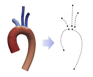
We use a patient-specific aorta model to demonstrate the accuracy and effectiveness of the analytic solution. The model is from an open-source dataset (BodyParts3D 2011) and is shown in figure 12. It includes the aorta and three main branches and is broken into individual sections indicated by the dashed lines for analytic modelling. The parameters used in each section are also listed in the figure. The vessel length $l$ is defined as the length of the curved centreline. The variation of the material properties follows the linear relation in figure 1, i.e. $Eh=\beta r$ with $\beta =5.94 \times 10^{5}\ {\rm g}\ {\rm cm}^{-1} \ {\rm s}^{-2}$. A pulsatile velocity profile with $T=0.9$ s is prescribed at AAo, and RCR boundary conditions are applied at all of the outlets. In CMM simulations, a grid independence study is carried out and around $0.5 \times 10^6$ tetrahedral elements are used to obtained the final results. Based on the Womersley number ($Wo=r \sqrt {2{{\rm \pi} } \rho f/\mu } \approx 16$) and the Reynolds number defined with Stokes layer thickness ($Re_{\delta }=\sqrt {2\rho }v_{max}/\sqrt {\mu \omega } \approx 195$), the flow has not transitioned to turbulence under the conditions considered here (Merkli & Thomann 1975; Hino, Sawamoto & Takasu 1976).

Figure 12. Patient-specific aorta model and the parameters used in the study. The dashed lines indicate all the sections of arteries used in the analytic model; AAo, ascending aorta; BCA, brachiocephalic artery; LCCA, left common carotid artery; LSUBA, left subclavian artery; DAo, descending aorta.

The flow rate and pressure at the inlet and outlets are summarized in figure 13. It can be seen that analytic results are in good agreement with numerical results. The pressure distribution is particularly well-matched, as the maximum relative error is maintained below $2\,\%$ and the average relative error remains under $1\,\%$. The average relative error of the flow rate is less than $2.4\,\%$, while the maximum error is higher due to a slight phase difference between these two results. It is worth noting that analytic results can be obtained within 1 s on a desktop equipped with an Intel Core i9-12900 K processor, while 3-D simulations take approximately 20 min per cardiac cycle when run in parallel on 288 Intel Xeon Platinum 9242 cores. Therefore, the analytic solution provides a fast and accurate alternative to 3-D simulations in estimating the pressure distribution in this model.

Figure 13. Comparison between the analytic solutions and 3-D simulation results for the patient-specific aorta model.

6. Conclusion

In this study, we derive an analytic solution for pulse wave propagation in an arterial model using frequency domain analysis. In addition to tapering, this model also includes variable wall properties that follow the profile $Eh=\beta r^\alpha$ and a physiological RCR outlet boundary condition that models the resistance and compliance of the downstream vascular network. This analytic solution is successfully validated against 1-D and 3-D numerical simulations. Then, it is used to theoretically analyse the wave propagation characteristics in an idealized model. It is confirmed that tapering and variable wall properties can create constant reflections along the path. Our study also demonstrates that wall properties and a RCR boundary condition have a significant impact on the wave propagation, and their influences are particularly prominent at the low-frequency range. Even though it is observed in figure 8 that high-frequency components are also affected by these factors, it is essential to approach these findings with caution, as viscous effects are not considered in the current model. Furthermore, it is worth noting that these high-frequency components may not hold significant physiological relevance, given the intrinsic frequency of the cardiac cycle.

Moreover, the analytic solution is applied to rapidly and accurately estimate the pressure distribution in a patient-specific aorta by splitting the model into individual sections and applying the analytic solution to each section. Compared with numerical methods, the analytic solution can be a computationally economical alternative for modelling pulse wave propagation. It also enables theoretical analysis to quantify the influence of different model parameters, such as boundary conditions and material properties, thus allowing for quick tuning of these parameters, which can then be used in 1-D and 3-D numerical simulations. Additionally, this method is potentially useful for clinical applications such as the estimation of the central pressure from peripheral pressure measurements. Building upon the study by Flores et al. (2021), it is possible to model the pressure wave propagation from the aorta to the brachial artery using the current analytic solution and derive a transfer function between central and brachial pressure.

There are several limitations in the current study. First, the omission of the nonlinear term (except for the steady component) and blood viscosity in the momentum equation leads to the under-estimation of pressure values. Reymond et al. (2009) demonstrated that both effects contributed approximately single-digit percentages to the predicted pressure value. Given that the errors we observe are of the same order of magnitude, including these effects can potentially improve our results. This is especially important in predicting pulse wave propagation within a long artery network with multiple layers of bifurcations, in which case avoiding error accumulation is of greater importance. Second, the blood vessel is more accurately modelled as a viscoelastic material. Experimental evidences have shown that there is hysteresis between pressure and lumen area (Valdez-Jasso et al. 2009) and the viscoelasticity causes attenuation of pulse waves as they travel downstream (Bessems et al. 2008). Last but not least, the current model cannot be applied directly to diseased arteries such as those with an aneurism or stenosis, but can potentially be expanded to model these anomalies (Papadakis & Raspaud 2019).